Many-body physics of slow light

Abstract

We present a quantum theory of slow light beyond the weak probe pulse approximation. By reduction of the full Hamiltonian of the system to an effective Hamiltonian for a single quantum field we demonstrate that the concept of dark-state polaritons can be introduced even if the linearized approach is no longer valid. The developed approach allows us to study the evolution of non-classical quantum states of the polariton field.

I Introduction

Slow light is a phenomenon associated with a propagation of dark-state polaritons Lukin1 ; Lukin2 , i.e., quantum superpositions of photons and spin excitations in a three-level medium [see Fig. 1  (a)], where a low-frequency coherence is established Harris1 , at the group velocity by many orders of magnitude less than the speed of light. The slow group velocity is attained via steep dispersion of the refractive index of the medium within the slow-light propagation window. Slow propagation of light pulses increases their interaction time and is therefore a key component of various proposed nonlinear-optical schemes aimed at the operation at the few-photon level propfew . Adiabatic switching off the coupling field maps the photon state onto the collective spin state Lukin4 , thus providing a reversible quantum memory.

Up to now the quantum aspects of the slow light propagation have been analyzed in the approximation, where the number of excitations in a medium is much less than the number of atoms Lukin1 ; Lukin2 . This approximation makes the construction of bosonic operators for dark-state polaritons easy and certainly holds for the case of experiments with atomic vapors in a gas cell expcell or large ensembles of cold atoms expMOT . Attempts to develop a quantum theory of slow light beyond the framework of Refs. Lukin1 ; Lukin2 have been scarce up to now beyond1 ; beyond2soliton and the analysis of the models has proved itself to be quite difficult. Remarkably, the approach of Ref. Kuang yielded definite results on the slow-light dynamics only in the semiclassical limit, and left open the question about the medium response to non-classical fields.

It is intuitively clear that, when the number of photons entering the medium becomes comparable to the number of atoms interacting with the light, the picture of dark-state polaritons with bosonic properties needs a more elaborate justification. The probe field interacts with a depleted medium and propagates at a velocity approaching the speed of light as the ratio of the input photons to the number of atoms increases. And a system that makes this situation experimentally feasible is now available. Thousands AR1 or hundreds (or tens) Kimble1 of atoms can be trapped near a single-mode tapered optical nanofiber and coupled via evanescent field to a probe (P) radiation sent through the nanofiber. A similar physical situation can be achieved also for atoms in hollow-core fibers hcf .

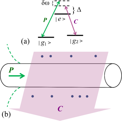
Figure 1: (Color Online). (a) The three-level excitation scheme of a slow-ligh esperiment: $|g_{1}\rangle$ and $|g_{2}\rangle$ are ground state sublevels, $|e\rangle$ is an optically excited state. (b) Sketch of the atoms trapped near a nanofiber. The probe light is transmitted through the nanofiber (the dashed line shows its evanescent field that excites atoms). The coupling field is sent perpendicularly to the nanofiber.

To simplify the analysis, we assume that the classical coupling (C) field is sent perpendicularly to the nanofiber, as shown in Fig. 1  (b). This allows us to assume the Rabi frequency $\Omega_{\mathrm{C}}$ for the atomic transition driven by the coupling field to be constant along the nanofiber. The case of co-propagating, nanofiber-guided, quantized probe and coupling fields requires a more elaborate treatment and is beyond the scope of the present paper.

The purpose of the present paper is to establish a many-body quantum theory of slow light for arbitrary probe light intensity, in other words, to formulate the problem as an effective Hamiltonian problem for a single bosonic field of dark-state polaritons beyond the linearized approach of Refs. Lukin1 ; Lukin2 . Although atoms in the system of interest do not interact with each other via short-range forces, nevertheless, they interact with each other via the nanofiber-guided electromagnetic field. Also we can say that probe-field photons interact with each other via their coupling to the atomic medium. As a result, the collective field of dark-state polaritons emerges, in some analogy to collective excitations in Bose-Einstein condensates of weakly-interacting atoms PethickSmith . This allows us to regard our theory as a many-body theory.

In Sec. II we introduce the full Hamiltonian of the problem and recover, by its diagonalization in the single-excitation case, the weak-field limit Lukin1 ; Lukin2 for the group velocity of dark-state polaritons. In Sec. III we recall the mean-field limit and the result of Kuang . The derivation of the effective Hamiltonian for dark-state polaritons beyond the linearized (weak-field) approach is presented in Sec. IV. The analysis of the dynamics of non-classical states of the dark-state polariton field described by this effective Hamiltonian is the subject of Sec. V.

II The full Hamiltonian

We consider a one-dimensional (1D) system of $N$ three-level atoms, $|g_{1}\rangle$ and $|g_{2}\rangle$ being the ground state sublevels and $|e\rangle$ being an optically excited state. The classical coupling field is detuned from the $|g_{2}\rangle\leftrightarrow|e\rangle$ transition by the frequency $\Delta$ (we explicitly write this detuning for the sake of generality; however, our approach works also in the case $\Delta=0$). If the probe field has the frequency $\omega$ then the two-photon detuning is $\delta\omega=\omega-\omega_{eg_{1}}-\Delta$, where $\omega_{eg_{1}}$ is the resonant frequency of the $|g_{1}\rangle\leftrightarrow|e\rangle$ transition, driven by the probe field. We use the slowly-varying amplitude approximation QO for the probe field, choosing $\omega_{0}=\omega_{eg_{1}}+\Delta$ as the carrier frequency. We assume the linear dispersion for the probe photons, $\omega=u|k|$, where $k$ is the wave number and $u$ is the velocity of propagation in the nanofiber. The operator of annihilation of a photon in a 1D nanofiber at the point $z$ at time $t$ is $\hat{\cal E}(z,t)\exp[-i\omega_{0}(t-z/u)]$. We introduce in a similar way the slowly varying amplitudes $\hat{\psi}_{1,2,e}$ for operators annihilating bosonic atoms in the states $|g_{1}\rangle$, $|g_{2}\rangle$, $|g_{e}\rangle$, respectively. Then the full Hamiltonian of the system in the interaction representation and in the rotating wave approximation reads as

$$\hat{H} = \hbar\int_{0}^{L}dz\,\Big{[}-iu\hat{\cal E}^{\dagger}\frac{\partial}{\partial z}\hat{\cal E}-\Delta\hat{\psi}_{e}^{\dagger}\hat{\psi}_{e}-\kappa(\hat{\cal E}^{\dagger}\hat{\psi}_{1}^{\dagger}\hat{\psi}_{e}+$$ (1)

$$\hat{\psi}_{e}^{\dagger}\hat{\psi}_{1}\hat{\cal E})-\Omega_{\mathrm{C}}(\hat{\psi}_{2}^{\dagger}\hat{\psi}_{e}+\psi_{e}^{\dagger}\hat{\psi}_{2})\Big{]}.$$

The periodic boundary conditions over the distance $L$ are assumed. We also recall that $\delta\omega=u\delta k$, where $\delta k=k-\omega_{0}/u$, reduces to $-iu\frac{\partial}{\partial z}$ when we write the slowly varying amplitude of the probe photonic field in the co-ordinate representation. The coupling between the probe field and the atoms is given by $\kappa=d_{eg_{1}}\sqrt{\omega_{0}/(2\hbar\varepsilon_{0}A)}$, where $d_{eg_{1}}$ is the projection of dipole moment of the atomic transition driven by the probe light to the unit vector of the probe field polarization, $\varepsilon_{0}$ is the dielectric permittivity of the vacuum in SI units, $A$ is the effective mode area determined by the structure of the evanescent field Aeff .

Both the atom-number

$$\hat{N}=\int_{0}^{L}dz\left(\hat{\psi}_{1}^{\dagger}\hat{\psi}_{1}+\hat{\psi}_{2}^{\dagger}\hat{\psi}_{2}+\hat{\psi}_{e}^{\dagger}\hat{\psi}_{e}\right)$$ (2)

and the excitation-number

$$\hat{M}=\int_{0}^{L}dz\left(\hat{\cal E}^{\dagger}\hat{\cal E}+\hat{\psi}_{2}^{\dagger}\hat{\psi}_{2}+\hat{\psi}_{e}^{\dagger}\hat{\psi}_{e}\right)$$ (3)

oprators commute with the Hamiltonian (1).

It is easy to show not only Eq. (2) holds, but also the operator of the local linear density of atoms is the integral of motion:

$$\frac{\partial}{\partial t}\left(\hat{\psi}_{1}^{\dagger}\hat{\psi}_{1}+\hat{\psi}_{2}^{\dagger}\hat{\psi}_{2}+\hat{\psi}_{e}^{\dagger}\hat{\psi}_{e}\right)=0.$$ (4)

Exact positions of atoms near the nanofiber are not essential for our treatment. Hence, we introduce atomic field operators using some kind of a coarse graining Lukin1 ; Lukin2 over length scales exceeding the mean interatomic separation in 1D. In what follows we assume that the linear density of atoms $n_{\mathrm{1D}}=N/L$ is not only continuous, but also spatially uniform,

$$\frac{\partial}{\partial z}n_{\mathrm{1D}}=0.$$ (5)

The Hamiltonian (1) can be easily diagonalized for $M=1$. However, it is more instructive to find the eigenvalue of Eq. (1) corresponding to the energy of a single dark-state polariton perturbatively, provided that the two-photon detuning is small enough, $|\delta\omega|\ll W_{\mathrm{sl}}$, where $W_{\mathrm{sl}}$ is the width of the slow-light propagation spectral window, discussed in the Appendix A. If the two-photon detuning is exactly zero, then the atomic medium is in the dark state $|\mathrm{DS}\rangle$ characterized by

$$\hat{\psi}_{e}|\mathrm{DS}\rangle=0,\quad\left(\kappa{\hat{\cal E}}\hat{\psi}_{1}+\Omega_{\mathrm{C}}\hat{\psi}_{2}\right)|\mathrm{DS}\rangle=0.$$ (6)

For small deviations from the two-photon resonance the energy $\hbar\omega^{\mathrm{DS}}_{\delta k}$ of the dark-state polariton can be calculated in the first order of the erturbation theory as

$$\hbar\omega^{\mathrm{DS}}_{\delta k}=u\delta k\langle\mathrm{DS}|\hat{\tilde{\cal E}}_{\delta k}^{\dagger}\hat{\tilde{\cal E}}_{\delta k}|\mathrm{DS}\rangle,$$ (7)

where

$$\hat{\tilde{\cal E}}_{\delta k}=\frac{1}{\sqrt{L}}\int_{0}^{L}dz\,\hat{{\cal E}}\exp(-i{\delta k}z).$$

Then the group velocity of a single dark-state polariton $v_{\mathrm{gr}}=\partial\omega^{\mathrm{DS}}_{\delta k}/(\partial\delta k)$ BornWolf yields the well-known weak-field limit Lukin1 ; Lukin2 :

$$v_{\mathrm{gr}}^{\mathrm{(w)}}=\frac{u\varrho}{1+\varrho},$$ (8)

where $\varrho={\Omega_{\mathrm{C}}^{2}/(\kappa^{2}n_{\mathrm{1D}})}$. If $\varrho\ll 1$, then the group velocity of the pulse is significantly slowed down compared to $u$.

III The mean-field limit

Heisenberg equations of motion for the electromagnetic and atomic field operators can be easily derived from Eq. (1) using bosonic commutation rules. Then we assume the semiclassical (mean-field) approximation and substitute the operators by classical complex fields thus obtaining the following set of evolution equations (the time derivative being denoted by a dot):

$$\dot{{\cal E}} = -u\frac{\partial}{\partial z}{\cal E}+i\kappa\psi_{1}^{*}\psi_{2},$$ (9)

$$\dot{\psi}_{1} = i\kappa{\cal E}^{*}\psi_{e},$$ (10)

$$\dot{\psi}_{e} = i\Delta\psi_{e}+i(\kappa{\cal E}\psi_{1}+\Omega_{\mathrm{C}}\psi_{2}),$$ (11)

$$\dot{\psi}_{2} = i\Omega_{\mathrm{C}}\psi_{e}.$$ (12)

Since in the slow-light regime the population of the optically excited state is negligibly small, we set

$$\kappa{\cal E}\psi_{1}+\Omega_{\mathrm{C}}\psi_{2}=0$$ (13)

[cf. Eq. (6)]. Eq. (13) and Eq. (12) rewritten as $\psi_{e}=-i\Omega_{\mathrm{C}}^{-1}\dot{\psi}_{2}$ reduce the number of independent variables to two. For them we obtain

$$\dot{{\cal E}}+\frac{\kappa^{2}}{\Omega_{\mathrm{C}}^{2}}\left(\psi_{1}^{*}\psi_{1}\dot{{\cal E}}+\psi_{1}^{*}{\cal E}\dot{\psi}_{1}\right) = -u\frac{\partial}{\partial z}{\cal E},$$ (14)

$$\dot{\psi}_{1}+\frac{\kappa^{2}}{\Omega_{\mathrm{C}}^{2}}\left({\cal E}^{*}{\cal E}\dot{\psi}_{1}+{\cal E}^{*}\psi_{1}\dot{{\cal E}}\right) = 0.$$ (15)

From Eq. (15) we obtain the conservation law for the atom number in the case, where all excitations are dark-state polaritons ($\psi_{e}^{*}\psi_{e}$ is negligible):

$$\psi_{1}^{*}\psi_{1}\left(1+\frac{\kappa^{2}}{\Omega_{\mathrm{C}}^{2}}{\cal E}^{*}{\cal E}\right)=n_{\mathrm{1D}}.$$ (16)

Substituting Eq. (16) and following from Eq. (15) expression

$$\dot{\psi}_{1}=-\frac{\kappa^{2}{\cal E}^{*}\psi_{1}\dot{\cal E}}{{\Omega_{\mathrm{C}}^{2}}+{\kappa^{2}}{\cal E}^{*}{\cal E}}$$

into Eq. (14), we obtain

$$\dot{\cal E}=-u\frac{({\Omega_{\mathrm{C}}^{2}}+{\kappa^{2}}{\cal E}^{*}{\cal E})^{2}}{\Omega_{\mathrm{C}}^{2}\kappa^{2}n_{\mathrm{1D}}+({\Omega_{\mathrm{C}}^{2}}+{\kappa^{2}}{\cal E}^{*}{\cal E})^{2}}\frac{\partial}{\partial z}{\cal E}.$$ (17)

Hence, we obtained the propagation equation with the intensity-dependent group velocity of Ref. Kuang .

The intensity dependence of the group velocity has been studied in different contexts nn . It manifests itself in wave front sharpening and, ultimately, in wave breaking ZaslUFN1 .

IV Derivation of the effective Hamiltonian for dark-state polaritons

The mean-field Eqs (14, 15) will be the starting point of our further derivations. We will reformulate the corresponding problem first in a Lagrangian and then in a Hamiltonian way. The resulting classical Hamiltonian will be again quantized and the quantum field for dark-state polaritons will be introduced. Such a method based on reduction of an exact many-body quantum problem to a set of classical Hamilton equations for certain collective variables and subsequent quantization of these collective variables proved itself to be successful in many studies, from the well-known quantization of phonons in solids SolidSt to the theory of macroscopic quantum tunneling of a Bose-Einstein condensate with attractive interactions MQT .

IV.1 Classical variables and the effective Hamiltonian

In what follows we use the Lagrangian and Hamiltonian formalisms for continuous systems described in detail, e.g., in Ref. Goldstein . We introduce the four generalized co-ordinates $J,\,S,\,\Xi,\,Q$ as real classical fields dependent on $z$ and $t$ via

$${\cal E}=\sqrt{J}\exp(-iS/\hbar),\quad{\psi_{1}}=\sqrt{{\Xi}}\exp(-iQ/\hbar).$$ (18)

Obviously, $J\geq 0$ and $\Xi\geq 0$. Planck’s constant appears in Eq. (18) in anticipation of the quantization of the variables in the next Subsection. Then the two complex Eqs. (14, 15) are transformed into four real equations

$$\dot{S}+\frac{\kappa^{2}}{\Omega_{\mathrm{C}}^{2}}\Xi(\dot{S}+\dot{Q}) = -u\frac{\partial}{\partial z}S,$$ (19)

$$\dot{J}+\frac{\kappa^{2}}{\Omega_{\mathrm{C}}^{2}}(\Xi\dot{J}+J\dot{\Xi}) = -u\frac{\partial}{\partial z}J,$$ (20)

$$\dot{Q}+\frac{\kappa^{2}}{\Omega_{\mathrm{C}}^{2}}J(\dot{S}+\dot{Q}) = 0,$$ (21)

$$\dot{\Xi}+\frac{\kappa^{2}}{\Omega_{\mathrm{C}}^{2}}(\Xi\dot{J}+J\dot{\Xi}) = 0.$$ (22)

The Lagrangian $\Lambda\equiv\int_{0}^{L}dz\,{\cal L}$ is constructed in such a way that the Lagrangian equations

$$\frac{d}{dt}\frac{\delta{\Lambda}}{\delta\dot{q}}=\frac{\delta{\Lambda}}{\delta q}$$

where $\delta/(\delta q)$ stands for variational derivative or, equivalently,

$$\frac{d}{dt}\frac{\partial{\cal L}}{\partial\dot{q}}=\frac{\partial{\cal L}}{\partial q}$$ (23)

is satisfied for $q$ standing for $J,\,S,\,\Xi,\,Q$. This determines the Lagrangian density

$${\cal L}=uJ\frac{\partial}{\partial z}S+\left(J+\frac{\kappa^{2}}{\Omega_{\mathrm{C}}^{2}}J\Xi\right)\dot{S}+\left({\Xi}+\frac{\kappa^{2}}{\Omega_{\mathrm{C}}^{2}}J\Xi\right)\dot{Q}.$$ (24)

Note, that, due to the assumed periodic boundary conditions, integration by parts gives the result

$$\int_{0}^{L}dz\,J\frac{\partial}{\partial z}S=-\int_{0}^{L}dz\,S\frac{\partial}{\partial z}J,$$ (25)

which is used in derivation of Eq. (20) from Eq. (23).

Since only $\dot{S}$ and $\dot{Q}$, but not $\dot{J}$ and $\dot{\Xi}$ appear in Eq. (24), we introduce two generalized momenta

$$P_{S} = \frac{\partial}{\partial\dot{S}}{\cal L}=J+\frac{\kappa^{2}}{\Omega_{\mathrm{C}}^{2}}J\Xi,$$ (26)

$$P_{Q} = \frac{\partial}{\partial\dot{Q}}{\cal L}=\Xi+\frac{\kappa^{2}}{\Omega_{\mathrm{C}}^{2}}J\Xi.$$ (27)

Eq. (22) then reduces to $\dot{P}_{Q}=0$, where $P_{Q}$ has the meaning of the linear density of atoms in the mean-field limit under the slow-light propagation conditions, i.e., $P_{Q}=n_{\mathrm{1D}}$.

From Eq. (13) we understand that $P_{S}$ is the sum of the densities of the photons and atoms driven from the state $|g_{1}\rangle$ to $|g_{2}\rangle$ under the slow-light propagation conditions (without populating the optically excited state), i.e., the density of dark polaritons in the mean-field regime. Bright polaritons Lukin2 , excitations appearing when the condition (13) is not fulfilled, do not contribute to the value of $P_{S}$.

Since $n_{\mathrm{1D}}$ is assumed to be spatially uniform [see Eq. (5)], the introduction of the effective Hamiltonian

$$H_{\mathrm{eff}} = \int_{0}^{L}dz\,(P_{S}\dot{S}+P_{Q}\dot{Q}-{\cal L})$$ (28)

$$= -u\int_{0}^{L}dz\,J(P_{S},P_{Q})\frac{\partial}{\partial z}S$$

easily yields the set of equations for the canonical variables

$$\dot{S} = \frac{\delta H_{\mathrm{eff}}}{\delta P_{S}}=-u\frac{\partial J(P_{S},P_{Q})}{\partial P_{S}}\frac{\partial S}{\partial z},$$ (29)

$$\dot{Q} = \frac{\delta H_{\mathrm{eff}}}{\delta P_{Q}}=-u\frac{\partial J(P_{S},P_{Q})}{\partial P_{Q}}\frac{\partial Q}{\partial z},$$ (30)

$$\dot{P}_{S} = -\frac{\delta H_{\mathrm{eff}}}{\delta S}=-u\frac{\partial J(P_{S},P_{Q})}{\partial P_{S}}\frac{\partial P_{S}}{\partial z},$$ (31)

$$\dot{P}_{Q} = -\frac{\delta H_{\mathrm{eff}}}{\delta Q}=0,$$ (32)

which is equivalent to Eqs. (19  –  22). Taking the non-negative solution of Eqs. (26, 27), we obtain

$$J(P_{S},P_{Q}) = \frac{1}{2}\left(P_{S}-P_{Q}-\frac{\Omega_{\mathrm{C}}^{2}}{\kappa^{2}}\right)+$$ (33)

$$\sqrt{\frac{1}{4}\left(P_{S}-P_{Q}-\frac{\Omega_{\mathrm{C}}^{2}}{\kappa^{2}}\right)^{2}+\frac{\Omega_{\mathrm{C}}^{2}}{\kappa^{2}}P_{S}}\,.~{}\,\,\,\,\,\,$$

After some algebra one can demonstrate the equivalence of Eqs. (29,   31) to Eq. (17).

From now on, we consider $P_{Q}\equiv n_{\mathrm{1D}}$ as a mere constant and treat the Hamiltonian given by Eqs. (28, 33) as a Hamiltonian for the canonical variables $S$ and $P_{S}$ only.

By introducing the complex field

$$\Psi=\sqrt{P_{S}}\exp(-iS/\hbar)$$ (34)

we can rewrite Eq. (29, 31) as

$$\frac{\partial}{\partial t}\Psi+v_{\mathrm{gr}}\frac{\partial}{\partial z}\Psi=0,$$ (35)

where

$$v_{\mathrm{gr}}=\frac{u}{2}\left[1+\frac{\frac{P_{S}}{n_{\mathrm{1D}}}-1+\varrho}{\sqrt{\left(\frac{P_{S}}{n_{\mathrm{1D}}}-1+\varrho\right)^{2}+4\varrho}}\right]$$ (36)

has the meaning of the intensity-dependent propagation velocity (group velocity) ZaslUFN1 ; NLW of dark-state polaritons and $\varrho=\Omega_{\mathrm{C}}^{2}/(\kappa n_{\mathrm{1D}})$ has to be much less than 1 to provide the slowdown of the propagation velocity of a weak pulse. After some algebra Eq. (36) can be expressed in terms of the probe-field Rabi frequency $\Omega_{\mathrm{P}}=\kappa\sqrt{J}$, thus reproducing the result of Ref. Kuang : $v_{\mathrm{gr}}=(\Omega_{\mathrm{P}}^{2}+\Omega_{\mathrm{C}}^{2})^{2}/[(\Omega_{\mathrm{P}}^{2}+\Omega_{\mathrm{C}}^{2})^{2}+\Omega_{\mathrm{C}}^{2}\kappa^{2}n_{\mathrm{1D}}]$. The limit $P_{S}\rightarrow 0$ yields the well-known result Eq. (8) in the weak-field limit Lukin1 ; Lukin2 .

IV.2 Quantization of the effective Hamiltonian

In quantum theory, the canonic variables $S$ and $P_{S}$ can be replaced with operators $\hat{S}$ and $\hat{P}_{S}$ obeying the commutation relation

$$[\hat{S}(z),\hat{P}_{S}(z^{\prime})]=i\hbar\delta(z-z^{\prime}).$$ (37)

In principle, we could define a quantum field for dark-state polaritons using the analogy with the phase-density representation of the atomic field in the theory of degenerate gases of bosonic atoms MoraCastin . Note that the sign of the commutator (37) is opposite to the widely used convention MoraCastin , since it was natural to introduce $S$ in Subsec. IV.1 as a generalized co-ordinate; the standard definition of the phase and density operators implies choosing $P_{S}$ as a generalized co-ordinate and $-S$ as a generalized momentum. However, the phase-density representation is well defined on the length scales containing on average many field quanta. This is not a problem in theory of atomic Bose-Einstein condensates or quasicondensates MoraCastin , but our goal is to formulate the theory in a way suitable for both small and large numbers of dark-state polaritons.

We take therefore one more step in our classical treatment by transforming $S,\,P_{S}$ to new canonic variables

$$\psi_{S}=\sqrt{2\hbar P_{S}}\sin(S/\hbar),\quad\psi_{P}=\sqrt{2\hbar P_{S}}\cos(S/\hbar),$$ (38)

${\cal F}=-\frac{1}{2}\int_{0}^{L}dz\,\psi_{S}^{2}\cot(S/\hbar)$ being the generating function of the canonical transformation. Obviously, $\Psi=({\psi_{P}-i\psi_{S}})/{\sqrt{2\hbar}}$. And now we substitute the new canonic variables with the operators $\hat{\psi}_{S,P}$, which are Hermitian, since they correspond to the real-valued observables, and obey the canonical commutation rules

$${[\hat{\psi}_{S}(z),\hat{\psi}_{S}(z^{\prime})]} = [\hat{\psi}_{P}(z),\hat{\psi}_{P}(z^{\prime})]=0,$$

$${[\hat{\psi}_{S}(z),\hat{\psi}_{P}(z^{\prime})]} = i\hbar\delta(z-z^{\prime}).$$ (39)

Then, in correspondence to Eq. (34), we introduce the quantum field

$$\hat{\Psi}=\frac{\hat{\psi}_{P}-i\hat{\psi}_{S}}{\sqrt{2\hbar}},\quad\hat{\Psi}^{\dagger}=\frac{\hat{\psi}_{P}+i\hat{\psi}_{S}}{\sqrt{2\hbar}}$$ (40)

that obeys the bosonic commutation relations

$${[\hat{\Psi}(z),\hat{\Psi}(z^{\prime})]} = [\hat{\Psi}^{\dagger}(z),\hat{\Psi}^{\dagger}(z^{\prime})]=0,$$

$${[\hat{\Psi}(z),\hat{\Psi}^{\dagger}(z^{\prime})]} = \delta(z-z^{\prime}).$$ (41)

Recalling the physical meaning of $P_{S}$ as the semiclassical density of dark polaritons, we can identify $\hat{\Psi}(z)$ and $\hat{\Psi}^{\dagger}(z)$ with operators of annihilation and creation, respectively, of a dark-state polariton at the point $z$. The dark-state polariton density operator is, obviously, $\hat{m}_{\mathrm{1D}}(z)=\hat{\Psi}^{\dagger}(z)\hat{\Psi}(z)$, and $\hat{M}_{\mathrm{D}}=\int_{0}^{L}dz\,\hat{m}_{\mathrm{1D}}(z)$ is the operator of the total number of the dark-state polaritons with non-negative integer eigenvalues $M_{\mathrm{D}}$.

Since the Hamiltonian (1) reduces under the conditions (6) to $\hat{H}_{\mathrm{eff}}=\hbar u\int_{0}^{L}dz\,\hat{\cal E}^{\dagger}\left(-i\frac{\partial}{\partial z}\right)\hat{\cal E}$, we need to establish the relation between the probe field and dark-state polariton operators. A proper unitary transformation relates $\hat{\cal E}$ not only to $\hat{\Psi}$, but also to the field operator for bright-state polaritons Lukin2 and, in a general case, to the excitations of the type that gradually approaches $\hat{\psi}_{e}$ as the atom-field coupling vanishes. But dark state polaritons are decoupled from excitations of other types in the limit of adiabatically slow dynamics discussed in the Appendix A. Hence, we assume that only dark-state polaritonic excitations are present in the system, $M\equiv M_{\mathrm{D}}$, and relate $\hat{\cal E}$ to $\hat{\Psi}$. We assume this relation is local, i.e., contains only dark-state polariton density operator in a given point. The locality property helps us to infer this relation from an easily solvable case of $M_{\mathrm{D}}$ dark state polaritons created by coupling to the medium probe photons exactly at the two-photon resonance. We make our notation of the dark state more definite and explicitly write the atom, $N$, and dark-state polariton, $M_{\mathrm{D}}$, quantum numbers. We introduce the annihilation operators $\hat{a}_{q}$ for probe photons and $\hat{d}_{q}$ for dark-state polaritons in the momentum modes via the plane wave expansions $\hat{\cal E}=\sum_{q}\hat{a}_{q}\exp(iqz)/\sqrt{L}$ and $\hat{\Psi}=\sum_{q}\hat{d}_{q}\exp(iqz)/\sqrt{L}$. Then the dark state $|\mathrm{DS};\,N,\,M_{\mathrm{D}}\rangle=(M_{\mathrm{D}}!)^{-1/2}d_{0}^{{\dagger}\,M_{\mathrm{D}}}|0\rangle$, where $|0\rangle$ is the vacuum of polaritons, can be expressed, according to Eq.(6), as a superposition of products of Fock states of atoms in the states $|g_{1}\rangle$, $|g_{2}\rangle$ and of probe photons:

$$|\mathrm{DS};\,N,\,M_{\mathrm{D}}\rangle = \frac{1}{\sqrt{{\cal A}_{N,M_{\mathrm{D}}}}}\sum_{m=0}^{m_{\max}}(-1)^{m}\left(\frac{\kappa}{\Omega_{\mathrm{C}}\sqrt{L}}\right)^{m}\times$$ (42)

$$\sqrt{\frac{(-N)_{m}(-M_{\mathrm{D}})_{m}}{m!}}\times$$

$$|N-m\rangle_{g_{1}}|m\rangle_{g_{2}}|M_{\mathrm{D}}-m\rangle_{\mathrm{phot}},~{}$$

where

$$(X)_{m}=\left\{\begin{array}[]{ll}1,&m=0\\ \prod_{j=1}^{m}(X+j-1),&m=1,\,2,\,3,\,\dots\end{array}\right.$$

is the Pochhammer symbol, $m_{\max}={\min(N,M_{\mathrm{D}})}$, and the normalization factor is

$${\cal A}_{N,M_{\mathrm{D}}}=\sum_{m=0}^{m_{\mathrm{max}}}\frac{(-N)_{m}(-M_{\mathrm{D}})_{m}}{m!}\left(\frac{\kappa^{2}}{\Omega_{\mathrm{C}}^{2}{L}}\right)^{m}.$$ (43)

It is easy to show that

$$\hat{a}_{0}|\mathrm{DS};\,N,\,M_{\mathrm{D}}\rangle = \sqrt{{\cal Y}_{N,M_{\mathrm{D}}}}\sqrt{M_{\mathrm{D}}}|\mathrm{DS};\,N,\,M_{\mathrm{D}}-1\rangle$$ (44)

$$= \sqrt{{\cal Y}_{N,M_{\mathrm{D}}}}\hat{d}_{0}|\mathrm{DS};\,N,\,M_{\mathrm{D}}\rangle,$$

where

$${\cal Y}_{N,M_{\mathrm{D}}}=\frac{{\cal A}_{N,M_{\mathrm{D}}-1}}{{\cal A}_{N,M_{\mathrm{D}}}}.$$ (45)

After some identical transformations we arrive at the following equation for ${\cal Y}_{N,M_{\mathrm{D}}}$:

$${\cal Y}_{N,M_{\mathrm{D}}}=\frac{\kappa^{-2}\Omega_{\mathrm{C}}^{2}L+({M_{\mathrm{D}}-1}){\cal Y}_{N-1,M_{\mathrm{D}}-1}}{N+\kappa^{-2}\Omega_{\mathrm{C}}^{2}L+({M_{\mathrm{D}}-1}){\cal Y}_{N-1,M_{\mathrm{D}}-1}}.$$ (46)

This exact equation can be used for recursive calculation of ${\cal Y}_{N,M_{\mathrm{D}}}$ for increasing numbers of dark-state polaritons, starting from

$${\cal Y}_{N,1}=\frac{\kappa^{-2}\Omega_{\mathrm{C}}^{2}L}{N+\kappa^{-2}\Omega_{\mathrm{C}}^{2}L}.$$ (47)

On the other hand, we can make an assumption

$${\cal Y}_{N,M_{\mathrm{D}}}\approx{\cal Y}_{N-1,M_{\mathrm{D}}-1},$$ (48)

whose consisteny is easily checked a posteriori. Then Eq. (46) reduces to a quadratic algebraic equation. Taking its positive root, we obtain

$${\cal Y}_{N,M_{\mathrm{D}}}\approx K\left(\frac{M_{\mathrm{D}}-1}{L},\frac{N}{L}\right),\quad K(P_{S},P_{Q})=\frac{J(P_{S},P_{Q})}{P_{S}},$$ (49)

and the function $J(P_{S},P_{Q})$ is defined by Eq. (33). Note that Eq. (49) reproduces Eq. (47) in the limit $M_{\mathrm{D}}=1$, where we take $K=\lim_{P_{S}\rightarrow 0}[J(P_{S},N/L)/P_{S}]={\kappa^{-2}\Omega_{\mathrm{C}}^{2}L}/({N+\kappa^{-2}\Omega_{\mathrm{C}}^{2}L})$, recalling that all the variables in Eq. (33) are non-negative by definition.

As we can see from Fig. 2, Eq. (48) provides a very good approximation for $M_{\mathrm{D}}-1<N$. The difference $D_{K}$ between the exact value of ${\cal Y}_{N,M_{\mathrm{D}}}$ and its approximation by Eq. (48) steeply rises near $(M_{\mathrm{D}}-1)/N=1$ to its maximum value $D_{K}^{\mathrm{max}}\sim 1/N$ and decreases slowly as $M_{\mathrm{D}}$ grows further. Such a deviation is, however, not important, since it is small compared to the limiting value of 1, which is rapidly approached by ${\cal Y}_{N,M_{\mathrm{D}}}$ as $\frac{M_{\mathrm{D}}-1}{N}$ begins to exceed unity by more than $2\sqrt{\varrho}$. For pulses of finite spatial extension $\ell_{\mathrm{p}}$ in the medium, we estimate the maximum systematic error of our approximation (49) as $D_{K}^{\mathrm{max}}\sim 1/(\ell_{\mathrm{p}}n_{\mathrm{1D}})$, which is always much less than unity, since by our course-graining assumption there are many atoms on a typical length scale of the problem.

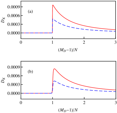
Figure 2: (Color Online). Difference $D_{K}={\cal Y}_{N,M_{\mathrm{D}}}-K\left(\frac{M_{\mathrm{D}}-1}{L},\frac{N}{L}\right)$ between the exact value of ${\cal Y}_{N,M_{\mathrm{D}}}$ defined by Eq. (45) and its approximation (49) for $\varrho=10^{-6}$ (a) and $10^{-4}$ (b); $N=1000$ (solid line) and 2000 (dashed line). Units on the axes are dimensionless.

Using Eq. (49) we obtain

$$\hat{\cal E}\hat{\varpi}_{\mathrm{D}}=\sqrt{K(\hat{\Psi}^{\dagger}\hat{\Psi},n_{\mathrm{1D}})}\,\hat{\Psi},$$ (50)

where $\hat{\varpi}_{\mathrm{D}}=\sum_{M_{\mathrm{D}}=0}^{\infty}|\mathrm{DS};\,N,\,M_{\mathrm{D}}\rangle\langle\mathrm{DS};\,N,\,M_{\mathrm{D}}|$ is the projection operator to the Hilbert subspace containing only dark-polariton states. Placing $\sqrt{K}$ to the left from the dark-polariton annihilation operator enables us to substitute $(M_{\mathrm{D}}-1)/L$ by the operator of the local density of dark-state polaritons $\hat{\Psi}^{\dagger}\hat{\Psi}$ in the first argument of $K$. Finally, the quantum effective Hamiltonian for dark-state polaritons is

$$\hat{H}_{\mathrm{eff}} = \hbar u\int_{0}^{L}dz\,\hat{\Psi}^{\dagger}\sqrt{K(\hat{\Psi}^{\dagger}\hat{\Psi},n_{\mathrm{1D}})}\times$$ (51)

$$\qquad\left(-i\frac{\partial}{\partial z}\right)\sqrt{K(\hat{\Psi}^{\dagger}\hat{\Psi},n_{\mathrm{1D}})}\,\hat{\Psi}.$$

V Results and discussion

The most interesting application of the theory developed in the previous section concerns the dynamics of non-classical states, which is hardly accessible by the methods developed previously Kuang . We can easily generalize the variational approach PethickSmith to these states. We assume a probe state $|{\chi}\rangle$ characterized by certain variational parameters and find an extremum

$$\delta{\cal S}_{\chi}=0$$ (52)

of the action

$${\cal S}_{\chi}=\langle\chi|\int_{t_{1}}^{t_{2}}dt\left(i\hbar\int_{0}^{L}dz\,\hat{\Psi}^{\dagger}\frac{\partial}{\partial t}\hat{\Psi}-\hat{H}_{\mathrm{eff}}\right)|\chi\rangle.$$ (53)

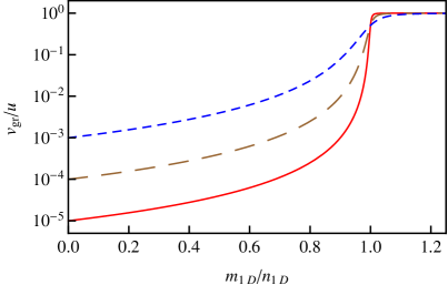
Figure 3: (Color Online). Group velocity of dark-state polaritons (normalized to the phase velocity $u$ of the probe light in the nanofiber) on the logarithmic scale as a function of the ratio of the dark-state polariton 1D density to the atomic 1D density. $\varrho=10^{-5}$ (solid line), $10^{-4}$ (long-dashed line), and $10^{-3}$ (short-dashed line). The units on the axes are dimensionless.

An exemplary non-classical state is a Fock state. Assume that $M_{\mathrm{D}}$ dark polaritons occupy the same state corresponding to a wave packet with a slowly varying envelope $\Phi(z,t)$ (the normalization $\int_{0}^{L}dz\,|\Phi|^{2}=1$ is assumed), i.e., $|\chi\rangle=(M_{\mathrm{D}}!)^{-1/2}\hat{d}_{\Phi}^{{\dagger}\,M_{D}}|0\rangle$, where $|0\rangle$ is the polaritonic vacuum state and $\hat{d}_{\Phi}^{\dagger}$ creates a dark polariton in the wave-packet state. Then Eq. (52) reads explicitly as

$$\frac{\delta S_{\chi}}{\delta\Phi^{*}}=0,$$

which results in the evolution equation for the slowly-varying envelope

$$\frac{\partial}{\partial t}\Phi+v_{\mathrm{gr}}\frac{\partial}{\partial z}\Phi=0,$$ (54)

where $v_{\mathrm{gr}}$ is given by Eq. (36) with $P_{S}=(M_{\mathrm{D}}-1)|\Phi|^{2}\equiv m_{\mathrm{1D}}$. Eq. (54) can be solved by the characteristics method NLW ; char .

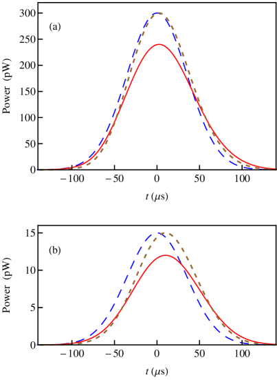
Figure 4: (Color Online). Power of the probe field at the entrance (long-dashed line) and at the exit (solid line) of the nanofiber-coupled atomic medium for a strong (a) and weak (b) pulse. See the system parameters in the text. Effects of absorption are taken into account according to Eq. (55). As a guide for eye, we show by a short-dashed line the pulse at the exit of the medium with fully neglected absorption [Eq. (51)]. In the case (a) the delay of the pulse peak arrival is negligible compared to the pulse peak delay of about 10 $\mu$s in the case (b).

Note that the propagation of the probe light intensity of the pulse is described by the essentially classical nonlinear group velocity even for a Fock state of dark-state polaritons, where $\langle\hat{\Psi}\rangle=0$. The number of probe photons is not well defined in this case, however, the state of the probe light is entangled with the state of the atomic medium [see Eq. (42)], and the average amplitude of the probe light is also zero. The absence of such coherences, contrary to the concerns of Ref. Kuang , does not change the dynamics dramatically, compared to the classical limit. This is not very surprising, since the optical coherence is shown to be a sufficient, but not necessary condition for observing many phenomena, traditionally associated with the semiclassical regime convf .

The group velocity shown in Fig. 3 exhibits rapid saturation at $v_{\mathrm{gr}}=u$ for $m_{\mathrm{1D}}>n_{\mathrm{1D}}$. Such a behavior can be associated with the depletion of the state $|g_{1}\rangle$ at too a high density of the dark-state polaritons: although the system remains in the dark state defined by Eq. (6), the average number of atoms available for coupling to the probe light becomes small, and probe photons pass through the medium without interaction-induced delay.

As an illustration, we present in Fig. 4 the results of numerical calculations of a slow-light pulse propagation through a nanofiber of a length $L=5000~{}\mu\mathrm{m}$. The linear density of cesium atoms Steck coupled to the nanofiber is $n_{\mathrm{1D}}=1~{}\mu\mathrm{m}^{-1}$, the effective area of the probe field mode $A=3~{}\mu\mathrm{m}^{2}$. We assume that the probe field drives the $|g\rangle=|F=4,\,M_{F}=4\rangle\leftrightarrow|e\rangle=|F^{\prime}=5,\,M_{F}^{\prime}=3\rangle$ transition of the cesium $D_{2}$-line. The phase velocity $u$ of light in the nanofiber is assumed to be of about 0.9 speed of light in vacuum; $\Omega_{\mathrm{C}}=3\times 10^{6}~{}\mathrm{s}^{-1}$.

Up to now, in our fully Hamiltonian theory we neglected the decay of the dark-state polaritons due to the small, but non-zero population of the optically excited state and coupling of the optical transitions to the free-space electromagetic modes. This assumption is valid if the two-photon detuning is less than the slow-light propagation spectral window, which is of the order of $\Omega_{\mathrm{C}}^{2}/(\gamma\sqrt{s})$ Harris1 ; Matisov1 for an optically dense ($s>1$) medium, where $2\gamma$ is the radiative decay rate of the optically excited state, $s=L/\zeta$ is the optical density of the medium, $\zeta=A/(n_{\mathrm{1D}}\sigma_{0})$ is Beer’s length, and $\sigma_{0}$ is the resonance cross-section of the probe light absorption.

Absorption effects can be accounted for by adding a corresponding non-adiabatic term Lukin2 to the propagation equation, which then reads as

$$\frac{\partial}{\partial t}\Psi+v_{\mathrm{gr}}\frac{\partial}{\partial z}\Psi=\frac{v_{\mathrm{gr}}^{3}\gamma^{2}}{2\zeta\Omega_{\mathrm{C}}^{4}}\frac{\partial^{2}}{\partial z^{2}}\Psi,$$ (55)

where by $\Psi$ we now denote the product of the normalized envelope function and the square root of the mean number of dark-state polaritons in the pulse. The expression $\Psi=\langle M_{\mathrm{D}}\rangle^{1/2}\Phi(z,t)$ is suitable in both the semiclassical and the Fock-state cases. The mean 1D density of probe photons is then approximately $|\Psi|^{2}K[(\langle M_{\mathrm{D}}\rangle-1)|\Phi|^{2},n_{\mathrm{1D}}]$. For the parameters of Fig. 4 ($s\sim 250$) absorption begins to play a role, but does not destroy the pulse too much. The delay time of the pulse peak arrival remains the same, the pulse becomes slightly broadened because of preferential absorption of its high-frequency components.

Generalizations of our variational theory in the spirit of multiconfigurational variational method Alon are possible, however, their development is out of the scope of the present paper.

To summarize, we developed a quantum many-body theory for the propagation of slow-light pulses. We developed a quantization framework that enabled us to introduce a bosonic quantum field for dark-state polaritons. The effective quantum Hamiltonian (51) is the main result of our work. We considered atoms coupled to a nanofiber as a definite example of an atomic medium, however, our results may be easily generalized to the cases of laser beam propagating in a gas cell or in an ultracold atomic cloud by replacing $A$ by the effective cross-section area of the probe beam. We found that the propagation of non-classical wave packets of slow light (Fock states of dark-state polaritons) is very similar to the classical dynamics in terms of light intensity. The existence of probe-field coherences is not necessary, contrary to the expectations of Ref. Kuang .

The author thanks A. Rauschenbeutel, C. Sayrin, Ph. Schneeweiß, and E. Shahmoon for helpful discussions. This work is supported by the Austrian Science Fund (FWF), project P 25329-N27.

Appendix A Spectral width of the slow-light propagation regime

The width $W_{\mathrm{sl}}$ of the slow-light propagation spectral window in optically dense ($s>1$) medium is well-known, see, e.g., the absorptive term in the bright-state polariton propagation equation in Ref. Lukin2 . Locally, the two-photon detuning couples the dark state to the bright state. The latter is coupled to the optically excited state and therefore has the width equal to the rate of induced transition to the optically excited state Matisov1 . If the two-photon detuning exceeds this width, the dark- and bright-states become mixed, and all effects based on the existence of the dark state decoupled from the optically excited state, including the slowing down of the probe pulse propagation, disappear. The effects of absorption in the medium further reduce this width by a factor of $1/\sqrt{s}$.

In this Appendix we consider in detail the case of a very large one-photon detuning, i.e., we consider the Hamiltonian (1) with $\Delta$ being the largest frequency available in the system; also $\Delta$ is assumed to be so large that the natural width of the optically excited state and the related effects of absorption of the probe photons can be neglected. We consider also, for the sake of clarity, states with a single excitation ($M=1$). We denote the states as follows: $|1\rangle$ is the state where all stoms are in their internal state $|g_{1}\rangle$ and one photon is present; in the state $|2\rangle$ there are no photons, but one atom is transferred from $|g_{1}\rangle$ to $|g_{2}\rangle$; the state with no photons and one atom excited to the state $|e\rangle$ is denoted by $|3\rangle$. Since the one-photon detuning is the highest frequency in this system, the state $|3\rangle$ can be adiabatically eliminated. For the probability amplitudes $a_{j}$, $j=1,2$, of the two remaining states we obtain the following Schrödinger equation:

$$i\frac{\partial}{\partial t}\left(\begin{array}[]{l}a_{1}\\ a_{2}\end{array}\right)=\left(\begin{array}[]{cc}\delta\omega+\frac{\kappa^{2}n_{\mathrm{1D}}}{\Delta}{}&\frac{\kappa\sqrt{n_{\mathrm{1D}}}\Omega_{\mathrm{C}}}{\Delta}\\ \frac{\kappa\sqrt{n_{\mathrm{1D}}}\Omega_{\mathrm{C}}}{\Delta}{}&\frac{\Omega_{\mathrm{C}}^{2}}{\Delta}\end{array}\right)\left(\begin{array}[]{l}a_{1}\\ a_{2}\end{array}\right).$$ (56)

We analyze the eigenvalues and eigenvectors of Eq. (56) depending on the two-photon detuning $\delta\omega=u\delta k$. The two states, denoted by superscripts $(\pm)$, and their respective eigenfrequencies are given by

$$\left(\begin{array}[]{l}a_{1}^{(+)}\\ a_{2}^{(+)}\end{array}\right)=\left(\begin{array}[]{l}\sin\vartheta\\ \cos\vartheta\end{array}\right),\quad\left(\begin{array}[]{l}a_{1}^{(-)}\\ a_{2}^{(-)}\end{array}\right)=\left(\begin{array}[]{r}\cos\vartheta\\ -\sin\vartheta\end{array}\right),$$ (57)

$$\omega_{\delta k}^{(\pm)} = \frac{1}{2}\left(\frac{\kappa^{2}n_{\mathrm{1D}}+\Omega_{\mathrm{C}}^{2}}{\Delta}+\delta\omega\right)$$ (58)

$$\pm\sqrt{\frac{1}{4}\left(\frac{\kappa^{2}n_{\mathrm{1D}}+\Omega_{\mathrm{C}}^{2}}{\Delta}+\delta\omega\right)^{2}-\frac{\Omega_{\mathrm{C}}^{2}\delta\omega}{\Delta}}\,,~{}~{}$$

where

$$\cot\vartheta=\frac{\Omega_{\mathrm{C}}}{\kappa\sqrt{n_{\mathrm{1D}}}}\left(1-\frac{\delta\omega}{\omega_{\delta k}^{(+)}}\right).$$ (59)

The dark-polariton state admitting the slow light propagation satisfies two conditions: (i) the derivative of its eigenfrequency over $\delta k$, i.e., the group velocity of the excitatio, is small compared to $u$ and (ii) the state adiabatically reduces to $|1\rangle$ when the ratio $\kappa\sqrt{n_{\mathrm{1D}}}/\Omega_{\mathrm{C}}$ is formally decreased to 0 (i.e., the coupling between $|g_{1}\rangle$ and $|e\rangle$ is switched off). Eqs. (57 —59) show that the state $|(-)\rangle$ possesses these properties for $|\delta\omega|\ll W_{sl}=({\kappa^{2}n_{\mathrm{1D}}+\Omega_{\mathrm{C}}^{2}})/|\Delta|$. Outside this spectral range either the group velocity is high (close to $u$) or the state does not reduce to $|1\rangle$ in the limit of the vanishing coupling between $|g_{1}\rangle$ and $|e\rangle$. In the latter case, a wave packet containing different photonic wave numbers and having adiabatically slowly changing envelop transforms, after entering the medium, into an excitation with the group velocity $\sim u$ with overwhelming probability.

If the one-phonon detuning is not too large, $|\Delta|\lesssim\sqrt{\kappa^{2}n_{\mathrm{1D}}+\Omega_{\mathrm{C}}^{2}}$, then the adiabaticity condition requires $|\delta\omega|\ll\sqrt{\kappa^{2}n_{\mathrm{1D}}+\Omega_{\mathrm{C}}^{2}}$ Lukin2 ; propfew ; nn .

References

- (1) M. Fleischhauer and M. D. Lukin, Phys. Rev. Lett. 84, 5094 (2000).
- (2) M. Fleischhauer and M. D. Lukin, Phys. Rev. A 65, 022314 (2002).
- (3) S. E. Harris, Physics Today, 50 (No. 7), 36 (1997).
- (4) S. E. Harris and L. V. Hau, Phys. Rev. Lett., 82, 4611 (1999); M. D. Lukin and A. Imamoǧlu, Phys. Rev. Lett. 84, 1419 (2000); Zeng-Bin Wang, K.-P. Marzlin, and B. C. Sanders, Phys. Rev. Lett. 97, 063901 (2006).
- (5) D. F. Phillips, A. Fleischhauer, A. Mair, R. L. Walsworth, and M. D. Lukin, Phys. Rev. Lett. 86, 783 (2001).
- (6) M. Shuker, O. Firstenberg, R. Pugatch, A. Ron, and N. Davidson, Phys. Rev. Lett. 100, 223601 (2008).
- (7) Bor-Wen Shiau, Meng-Chang Wu, Chi-Ching Lin, and Ying-Cheng Chen, Phys. Rev. Lett. 106, 193006 (2011).
- (8) I. Vadeiko, A. V. Prokhorov, A. V. Rybin, and S. M. Arakelyan, Phys. Rev. A 72, 013804 (2005).
- (9) A. Rybin and J. Timonen, Phil. Trans. Roy. Soc. 369, 1180 (2011).
- (10) Le-Man Kuang, Guang-Hong Chen, and Yong-Shi Wu, J. Opt. B 5, 341 (2003).
- (11) E. Vetsch et al., Phys. Rev. Lett. 104, 203603 (2010).
- (12) A. Goban et al., Phys. Rev. Lett. 109, 033603 (2012).
- (13) M. J. Renn et al., Phys. Rev. Lett. 75, 3253 (1995); C. A. Christensen et al., Phys. Rev. A 78, 033429 (2008); S. Vorrath, S. A. Möller, P. Windpassinger, K. Bongs, and K. Sengstock, New J. Phys. 12, 123015 (2010); M. Bajcsy et al., Phys. Rev. A 83, 063830 (2011).
- (14) C. J. Pethick and H. Smith, Bose Einstein Condensation in Dilute Gases (Cambridge University Press, Cambridge, 2008), Chapters 7, 8.
- (15) M.O. Scully and M.S. Zubairy, Quantum Optics (Cambridge University Press, Cambridge, 1997), Chapter 5.
- (16) Fam Le Kien, V. I. Balykin, and K. Hakuta, Phys.Rev.A 73, 013819 (2006).
- (17) M. Born and E. Wolf, Principles of Optics (Cambridge University Press, Cambridge, 2005), Chapter 1.
- (18) I. E. Mazets and B. G. Matisov, Quantum Semiclassical Opt. 8, 909 (1996); I. E. Mazets, Phys. Rev. A 54, 3539 (1996); M. Fleischhauer and A. S. Manka, Phys. Rev. A 54, 794 (1996).
- (19) G.M. Zaslavsky, Uspekhi Fiz. Nauk 111 (No. 3), 395 (1973) [Sov. Phys. Uspekhi 16, 761 (1974)].
- (20) N.W. Ashcroft and N.D. Mermin, Solid State Physics (Thomson Learning, South Melbourne, 1976), Chapters 22, 23.
- (21) M. Ueda and A. J. Leggett, Phys. Rev. Lett. 80, 1576 (1998).
- (22) H. Goldstein, C. Poole, and J. Safko, Classical Mechanics, 3rd ed. (Addison Wesley, New York, 2001), Chapter 13.
- (23) G.B. Witham, Linear and Nonlinear Waves (Wiley, NY, 1999), Chapters 5, 14, and 15.
- (24) C. Mora and Y. Castin, Phys. Rev. A 67, 053615 (2003).
- (25) K. Mølmer, Phys. Rev. A 55, 3195 (1997).
- (26) R. Courant and D. Hilbert, Methods of Mathematical Physics, Vol. II (Wiley, Singapore, 1962), Chapter 2.
- (27) The spectroscopic data of cesium are put together by D. Steck, http://steck.us/alkalidata/cesiumnumbers.1.6.pdf.
- (28) M.B. Gornyi, B.G. Matisov, and Yu.V. Rozhdestvenskii, Zh. Eksp. Teor. Fiz. 95, 1263 (1989) [Sov. Phys. JETP 68, 728 (1989)].
- (29) A. I. Streltsov, O. E. Alon, and L. S. Cederbaum, Phys. Rev. A 73, 063626 (2006); O. E. Alon, A. I. Streltsov, and L. S. Cederbaum, Phys. Rev. A 77, 033613 (2008).