Matching for balance, pairing for heterogeneity in an observational study of the effectiveness of for-profit and not-for-profit high schools in Chile

Abstract

Conventionally, the construction of a pair-matched sample selects treated and control units and pairs them in a single step with a view to balancing observed covariates $\mathbf{x}$ and reducing the heterogeneity or dispersion of treated-minus-control response differences, $Y$. In contrast, the method of cardinality matching developed here first selects the maximum number of units subject to covariate balance constraints and, with a balanced sample for $\mathbf{x}$ in hand, then separately pairs the units to minimize heterogeneity in $Y$. Reduced heterogeneity of pair differences in responses $Y$ is known to reduce sensitivity to unmeasured biases, so one might hope that cardinality matching would succeed at both tasks, balancing $\mathbf{x}$, stabilizing $Y$. We use cardinality matching in an observational study of the effectiveness of for-profit and not-for-profit private high schools in Chile—a controversial subject in Chile—focusing on students who were in government run primary schools in 2004 but then switched to private high schools. By pairing to minimize heterogeneity in a cardinality match that has balanced covariates, a meaningful reduction in sensitivity to unmeasured biases is obtained.

Matching for balance, pairing for heterogeneity in an observational study of the effectiveness of for-profit and not-for-profit high schools in Chile

,
and t1Supported in part by Grant 1110485 from Fondecyt and Grant SBS-1260782 from the US National Science Foundation.

1 Introduction

1.1 Educational test scores and school profits

In Chile, as in the US, Britain, Canada and elsewhere, some secondary schools are operated by the government and others are private enterprises that charge parents a fee to educate their children. In Chile, some of the private schools are not-for-profit enterprises, for instance, a school operated by a church, and others are for-profit enterprises not different in concept than a restaurant or retail store. Whether schools should be allowed to profit is an intensely controversial issue in Chile. On the one hand, supporters of for-profit schools argue that they have incentives for efficiency and innovation, and that this in turn results in better education. Opposing this view, detractors say that, in reducing costs, for-profit schools tend to also reduce the quality of education and that one cannot allow a desire for profits to take precedence over the quality of a child’s education [see Elacqua (2009) for further discussion]. In 2011, in support of the latter view, and in part with the goal of ending for-profit education in Chile, thousands of students rallied through the streets demanding a change in the model of education and better opportunities.

Here, we compare the 2006 academic test performance of Chilean students who entered for-profit private high schools and students who entered not-for-profit private high schools. All of these students were in government run primary/middle schools in Santiago in 2004 and subsequently moved to private high schools. We have test scores at baseline in 2004 in language (Spanish), mathematics, natural science and social science, and we have outcome test scores in 2006 in language and mathematics. In addition, we have extensive data about parents and children in 2004, such as the education of the parents, their income, the number of books at home and so on, recorded in an observed covariate $\mathbf{x}$. An obvious concern is that even after adjusting for a high-dimensional observed covariate $\mathbf{x}$, children in different types of schools may differ in terms of some other covariate $u$ that was not observed, and differences in $u$ may bias the comparison.

The test scores come from the SIMCE, the Spanish acronym for “System of Measurement of Quality in Education.” For the same students, we use test scores for the 8th grade of primary school in 2004 and the second year of high school in 2006. For the typical student, these are test scores at ages 14 and 16. For-profit and not-for-profit are determined by the official definitions of the Chilean IRS based on the institutional identification number (RUT).

Do profits boost or depress test scores in similar students? Or are profits irrelevant to test scores?

1.2 Matching for covariate balance, pairing for heterogeneity

To be credible, the comparison must compare children in not-for-profit schools (the treated group) to children similar at baseline in for-profit schools (the control group), and there are many ways the children may differ. It is typically difficult to match closely for all coordinates of a high-dimensional observed covariate $\mathbf{x}$, but it is often not difficult to create matched treated and control groups with similar distributions of $\mathbf{x}$. For instance, if $\mathbf{x}$ consisted of 20 binary covariates, it would distinguish $2^{20}$ or about a million categories of students, so it would be very difficult to match thousands of students exactly for all 20 covariates. However, it is not difficult to balance $\mathbf{x}$ in treated and control groups, for instance, by matching for an estimate of the one-dimensional propensity score, that is, for an estimate of the conditional probability of treatment given the observed covariates [Rosenbaum and Rubin (1983)]. The resulting matched pairs are heterogeneous in $\mathbf{x}$ but the heterogeneity in $\mathbf{x}$ is unrelated to treatment and so tends to balance out in the treated and control groups as whole groups. Randomized treatment assignment also balances covariates without eliminating heterogeneity in covariates, but of course randomization balances both observed covariates $\mathbf{x}$ and unobserved covariate $u$, whereas matching for the observed $\mathbf{x}$ cannot be expected to balance $u$. It is typically difficult to randomly assign students to schools, although it has happened in special situations.

If pairs matched for $\mathbf{x}$ have a not-for-profit-minus-for-profit matched pair difference $Y$ in outcome test scores that is not centered at zero, then the explanation may be an effect of not-for-profit-versus-for-profit schools or it may instead reflect some pretreatment difference in an unobserved covariate $u$. A sensitivity analysis in an observational study asks: what would $u$ have to be like to explain the observed behavior of $Y$ in the absence of a treatment effect? In the first sensitivity analysis, Cornfield et al. (1959) found that to explain away the observed association between heavy smoking and lung cancer as something other than an effect caused by smoking, the unobserved $u$ would need to be a near perfect predictor of lung cancer and an order of magnitude more common among smokers than nonsmokers. In Section 3.2, a closely related though considerably more general method of sensitivity analysis is reviewed.

It is known that the heterogeneity of $Y$, its dispersion around its center, affects the degree of sensitivity to unmeasured biases [Rosenbaum (2005)]; see Section 3.4 below. A typical effect of, say, $\tau$, will be more sensitive to an unobserved bias $u$ in treatment assignment if the $Y$’s are widely dispersed about $\tau$ and less sensitive if the $Y$’s are tightly packed around $\tau$, and this pattern will persist no matter how large the sample size becomes. In this sense, reducing the heterogeneity or dispersion of individual pair differences $Y$ is more important than increasing the sample size, because an increase in sample size has little to do with sensitivity to bias (or, more precisely, heterogeneity affects design sensitivity but sample size does not). The heterogeneity of the $Y$’s is partly determined by factors that the investigator cannot control, but often the investigator has some control. To some extent, the heterogeneity of $Y$ may be affected by the use of special populations, say, twins or siblings who happened to receive different treatments. To a limited extent, the heterogeneity of the pair differences, $Y$, is affected by how the pairing for $\mathbf{x}$ is done. Our goal in the current paper is to reduce sensitivity to unmeasured biases from $u$ by pairing in such a way that the heterogeneity of $Y$ is reduced.

Conventionally, matching for $\mathbf{x}$ and pairing for $\mathbf{x}$ are conceived as one task: treated and control groups are made similar as groups in terms of $\mathbf{x}$ by pairing treated and control individuals with similar $\mathbf{x}$’s. Using a new matching algorithm called “cardinality matching” in Section 2, we form matched treated and control groups that are of the largest proportional size possible (i.e., the maximum cardinality) such that the distributions of $\mathbf{x}$ are balanced in the groups as a whole. The result is either the maximum number of pairs possible subject to covariate balance constraints or the largest $L$-to-1 match using all treated individuals, again subject to covariate balance constraints. In other words, the marginal distributions of $\mathbf{x}$ in treated and control groups are constrained to be similar, and the maximum cardinality match is the largest proportional match that makes them similar. The algorithm that produces the maximum cardinality match is indifferent as to who is paired with whom; instead, it maximizes the size of a match that meets specified requirements for balance on $\mathbf{x}$; see (1) below. This is done using integer programming. Then, with the groups determined and fixed, pairs or $L$-to-1 matched sets are formed using minimum distance pair matching for a robust Mahalanobis distance computed from a few key coordinates of $\mathbf{x}$ with a view to reducing heterogeneity in the outcome within pairs or matched sets. An alternative approach is described in Section 2.5.

In the Chilean schools in Section 1.1, pairs are formed using test scores in 2004, so treated and control groups are balanced for all of $\mathbf{x}$ by maximum cardinality matching, yet individual pairs are also paired very closely for 2004 test scores by optimal pair matching. In other words, the treated and control groups have the same proportion of boys, the same proportion of mothers who completed secondary school and so on, so the treated and control groups look comparable as groups in terms of the measured covariates. However, the pairing is concerned with test scores in middle school, so a boy with good language scores and poor math scores may be paired with a girl with similar test scores.

Unlike cardinality matching, typical matching algorithms find matched groups that are balanced for $\mathbf{x}$ at the same time as they find pairs close on $\mathbf{x}$. In doing this, typical algorithms do not usually find the largest matched sample that balances observed covariates; after all, this is not the criterion that they optimize. Additionally, typical algorithms will balance gender by trying to pair boys with boys, even if gender is not a strong predictor of test performance in high school. If one is going to break up the initial pairing and pair the same individuals a second time (henceforth, if one is going to “re-pair”), then effort spent making the initial pairing close on $\mathbf{x}$ is effort wasted; after all, the initial pairing is not used. Cardinality matching is most attractive when a convincing comparison must balance many covariates, even though it is known that a small subset of the covariates is key for predicting the outcome. Cardinality matching is least attractive when there is no reason to think that some covariates or covariate summaries are much more important for prediction than others.

The key covariates for revised pairing are known before the study begins in many contexts. This is true, for example, of the baseline 2004 test scores in the Chilean schools in Section 1.1, and it is also true of clinical stage, grade and histology in some clinical cancer studies. In other contexts, there are widely used, extensively validated summary scores that could be used for the revised pairing, such as the APACHE score in clinical medicine [Knaus et al. (1985)] or the Charleson Index in health services research [Deyo, Cherkin and Ciol (1992)]. Obviously, one can match for both such a summary score and a few key covariates using some form of the Mahalanobis distance. Rubin (1979) found that covariance adjustment of matched pair differences is a particularly robust technique, being little affected by misspecification of the regression model, and his approach using all of $\mathbf{x}$ can additionally provide some insurance against an omission when identifying the key covariates for revised pairing. Sensitivity analysis after covariance adjustment of matched pairs is illustrated in Rosenbaum (2007).

Baiocchi (2011) proposed re-pairing any initial pair-matched sample by, first, using the unused, unmatched controls to estimate Hansen’s (2008) prognostic score, and, second, revising the initial pairing to be close on the estimated prognostic score, so that, after revision, pairs have similar predicted responses under control. Baiocchi’s revised match retains whatever balancing properties for $\mathbf{x}$ that the initial match may have had, because it uses the same treated and control groups, yet the new pairs are now close in terms of a prognostic score whose estimated weights came from data independent of the paired data that will be the basis for the study’s conclusion. A limited version of Baiocchi’s method would simply use the unused, unmatched controls to identify the most important covariates for predicting the outcome and then re-pair using those covariates directly. Baiocchi’s method concerns the second step, the revision of a balanced match, and it is a natural complement to cardinality matching that concerns the first step, namely, finding the largest balanced matched sample ignoring who is matched to whom. The key variables for revised pairing are known a priori in some contexts, but when this is not the case, Baiocchi’s method is a clever and useful strategy for revising the pairing of a balanced matched sample.

Reducing the dispersion or heterogeneity of pair differences $Y$ reduces sensitivity to unmeasured biases, but increasing the sample size does not. Is matching each treated subject to $L>1$ controls analogous to reducing heterogeneity or to increasing the sample size? Matching with more than one control often reduces sensitivity to unmeasured biases [Rosenbaum (2013)]. Stated informally, this occurs when an unmeasured covariate $u$ cannot both closely predict the pattern of outcomes among $L+1$ individuals in an $L$-to-1 matched set and also closely predict which one of $L+1$ individuals will receive the treatment. When possible, cardinality matching will automatically construct $L$-to-1 matched sets with the largest $L$ if this is consistent with balancing $\mathbf{x}$, and otherwise it will find the largest 1-to-1 pair matching that balances $\mathbf{x}$.

For recent surveys of multivariate matching, see Stuart (2010) and Lu et al. (2011).

1.3 Outline and key ideas

The remainder of the paper discusses and illustrates the following three topics.

A new method: The visible heterogeneity of responses within matched pairs affects the sensitivity of conclusions to unmeasured biases [Rosenbaum (2005)]. A new matching algorithm, cardinality matching, balances many covariates but pairs for just a few covariates that reduce the heterogeneity of matched pair differences in outcomes, thereby reducing sensitivity to unmeasured biases. Cardinality matching finds the largest match that meets the user’s specifications for covariate balance, also addressing the possibility of covariate distributions exhibiting limited overlap.

Recent developments: A poor choice of test statistic can lead to a mistaken view that an observational study is sensitive to small biases when it is not. We illustrate an adaptive choice of test statistic in sensitivity analysis [Rosenbaum (2012a)].

A case study: The case study of for-profit schools in Chile illustrates cardinality matching and the switch from a conventional match and analysis to an alternative guided by statistical theory produces a substantial reduction in reported sensitivity to unmeasured biases.

Section 2 describes the new matching algorithm and Section 3 is a review of recent developments in sensitivity analysis. Technical details may be avoided by focusing on the case study in Sections 2.2, 2.3, 2.6 and 4.

1.4 Aspects of the Chilean data

We compare test scores of students in Santiago who moved from a public primary school in 2004 to either a private for-profit or a private non-for-profit secondary school in 2006. The data are from the Education Quality Measurement System (SIMCE) which contains results from a standardized test given by the Ministry of Education to all the students in Chile in a given year. Unlike standardized educational tests in the US, the SIMCE tests every student in Chile and in this sense resembles a census rather than a sample or an administrative data set. After applying basic data exclusion criteria [namely, excluding from the analysis those students (i) who were not in Santiago, (ii) who did not move from a public primary school in 2004 to either a private for-profit or a non-for-profit secondary school in 2006, (iii) whose reported gender changed between years, or (iv) who had missing values in one of the baseline or outcome test scores], before matching we obtained data from students in 483 public primary schools in 2004. After matching, our matching algorithm selected students from 446 of these 483 public primary schools. The sample of matched students had students from 453 private secondary schools in 2006 (170 for-profit and 283 non-for-profit). Before matching there were 573 private secondary schools, 170 for-profit and 403 non-for-profit.

2 Cardinality matching followed by minimum distance pairing

2.1 Cardinality matching: The largest matched sample that balances covariates

Cardinality matching finds the largest match that balances observed covariates. Balancing observed covariates is expressed abstractly by $K$ linear inequalities in functions of the observed covariates. Just as it is convenient to describe linear regression abstractly, and then later observe that the abstract definition permits interactions, polynomials, some types of splines, nominal predictors, etc., so too it is convenient to describe covariate balance abstractly, and then observe that various ways of making the abstract statement tangible may be used to achieve a variety of desirable effects. For instance, the $K$ linear inequalities can balance proportions, means, variances, covariances, and a grid of quantiles of a marginal distribution, among many other effects.

There are initially treated units $\mathcal{T}=\{\rho_{1},\ldots,\rho_{T}\}$ and controls $\mathcal{C}=\{\kappa_{1},\ldots,\allowbreak\kappa_{C}\}$. Treated unit $\rho_{t}$ has observed covariate $\mathbf{x}_{\rho t}$, $t=1,\ldots,T$, and control $\kappa_{c}$ has observed covariate $\mathbf{x}_{\kappa c}$, $c=1,\ldots,C$. Let $a_{tc}=1$ if $\rho_{t}$ is initially matched to $\kappa_{c}$, with $a_{tc}=0$ otherwise. Each matched treated unit is to have the same number, $L\geq 1$, of matched controls, where the algorithm will make $L$ as large as possible subject to the requirement that the covariates be balanced in treated and control groups. More precisely, it will either find the largest match using all $T$ treated units each matched to $L$ distinct controls or it will find the 1-to-1 matching that uses the maximum number of treated units. A covariate balance constraint $\mathbb{B}_{k}$ is a linear inequality constraint

$$\mathbb{B}_{k}\dvtx-b_{k}\sum_{t=1}^{T}\sum_{c=1}^{C}a_{tc}\leq\sum_{t=1}^{T}\sum_{c=1}^{C}a_{tc}v_{ktc}\leq b_{k}\sum_{t=1}^{T}\sum_{c=1}^{C}a_{tc},$$ (1)

where $v_{ktc}$ is the $k$th of $K$ functions of observed covariates and $b_{k}\geq 0$ is a given constant. Specifically, $\mathbb{B}_{k}$ says the mean $(\sum_{t=1}^{T}\sum_{c=1}^{C}a_{tc}v_{ktc})/\allowbreak(\sum_{t=1}^{T}\sum_{c=1}^{C}a_{tc})$ of $v_{ktc}$ over matched units ($a_{tc}=1$) is in the interval $[-b_{k},b_{k}]$, and taking $b_{k}=0$ says the mean of $v_{ktc}$ over matched units ($a_{tc}=1$) is zero.

Many useful balance constraints have the form (1) with $v_{ktc}=f(\mathbf{x}_{\rho t})-f(\mathbf{x}_{\kappa c})$ for some function $f(\cdot)$. If $f(\cdot)$ is a binary indicator of whether $\mathbf{x}$ satisfies some condition, then (1) with $b_{k}=0$ forces the matched sample to have the same number of treated subjects satisfying this condition as controls satisfying this condition, without constraining who is matched to whom. The covariates gender, school type, categories of household income, and categories of mother’s and father’s education were exactly balanced in this way, a constraint known as “fine balance” [Zubizarreta et al. (2011)]. Fine balance for gender means that the proportion of boys is the same in the matched treated and control groups, but boys may be paired with girls. When several covariates are finely balanced, the mean of every linear combination of these covariates is also exactly balanced. A binary indicator $f(\cdot)$ with $b_{k}=0.01$, say, will limit the imbalance to at most a count of 1%, a condition known as “near fine balance” [Yang et al. (2012)]. The categories of “number of books at home” were nearly balanced in this way. In parallel, $f(\cdot)$ with $b_{k}=0$ may be used to balance the joint distributions of two or more nominal covariates, say, the gender of the student and the years of education of the mother. If $f(\cdot)$ simply picks out one coordinate of $\mathbf{x}$, then a pair of constraints of the form (1) forces the matched sample to have means in the treated and control groups that differ by at most $b_{k}$, say, that the mean test scores in natural science in 2004 are close. The student’s own four test scores in 2004 and the four average test scores in the student’s 2004 school were balanced on average in this way. If instead $f(\cdot)$ calculates the square of one coordinate or the cross-product of two coordinates, then a sequence of constraints of the form (1) can balance higher moments of the covariates. A binary indicator $f(\cdot)$ may be used to ensure that the same number or a similar number of treated subjects and controls have a value of one covariate below a particular number, and a sequence of such binary indicators may be used to force agreement between two empirical distribution functions at the grid of values. In Figure 1, the entire distribution of the sum of math and language scores in 2004 was balanced in this way. In an analogous way, constraints of the form (1) may be used to ensure that an estimated propensity score has a similar distribution in treated and control matched samples. Also, rather than eliminate subjects with missing covariates, one can force treated and control matched groups to exhibit similar patterns of missing covariates, say, 5% of a particular covariate being missing in both groups. For detailed discussion of the variety of statistical properties that may be induced through balance constraints of different types, see Zubizarreta (2012).

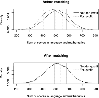
Figure 1: Total of language and mathematics scores at baseline in 2004, before and after cardinality matching. Vertical lines indicate quintiles.

The user of cardinality matching specifies $K$ constraints of the form (1). The goal is to find the largest $L$-to-1 match that satisfies the $K$ balance constraints, the largest match that balances all of the observed covariates. The result may be, say, a 3-to-1 match of all treated units, or it may be a 1-to-1 pair match discarding the smallest possible fraction of the treated units. In any case, the algorithm finds the largest $L$-to-1 match that exists subject to the $K$ constraints that define covariate balance. A cardinality matching is then the solution to the following several optimization problems. First, find $\mathbf{a}=(a_{11},a_{12},\ldots,a_{TC})$ as the solution to

$$\max\sum_{t=1}^{T}\sum_{c=1}^{C}a_{tc}$$

$$\mbox{subject to }a_{tc}\in\{0,1\},\qquad t=1,\ldots,T,c=1,\ldots,C,$$

$$\hskip 45.0pt\sum_{t=1}^{T}a_{tc}\leq 1\qquad\mbox{for }c=1,\ldots,C,$$ (2)

$$\hskip 45.0pt\sum_{c=1}^{C}a_{tc}\leq 1\qquad\mbox{for }t=1,\ldots,T,$$

$$\hskip 45.0pt\mathbb{B}_{k},\qquad k=1,\ldots,K.$$

In words, (2.1) is the largest pair-matched sample that meets the user’s $K$ balance constraints $\mathbb{B}_{k}$, $k=1,\ldots,K$ in (1). Specifically, $\sum_{t=1}^{T}\sum_{c=1}^{C}a_{tc}$ is the number of subjects in the treated and control groups, $\sum_{t=1}^{T}a_{tc}\leq 1$ says that control $c$ is used at most once, and $\sum_{c=1}^{C}a_{tc}\leq 1$ says treated unit $t$ is used at most once.

Having solved (2.1), there are two cases to consider. In case 1, the solution to (2.1) has $T=\sum_{t=1}^{T}\sum_{c=1}^{C}a_{tc}$, so that a pair match satisfying the balance constrains $\mathbb{B}_{k}$, $k=1,\ldots,K$ constraints has been found that uses all $T$ treated units. In this first case, the problem is solved again with the third constraint, $\sum_{c=1}^{C}a_{tc}\leq 1$ for $t=1,\ldots,T$, replaced by $\sum_{c=1}^{C}a_{tc}=L$ with $L=2$ for $t=1,\ldots,T$. If this second solution has $LT=2T=\sum_{t=1}^{T}\sum_{c=1}^{C}a_{tc}$, then a $2$-to-$1$ match satisfying the balance constrains $\mathbb{B}_{k}$, $k=1,\ldots,K$ constraints has been found, and the problem is solved again with $L$ replaced by $L+1$. For some $L$, $L=2$, $3,\ldots,$ the problem is infeasible, meaning that a match of $L$-to-$1$ cannot satisfy the balance constraints $\mathbb{B}_{k}$, $k=1,\ldots,K$. In this first case, the optimal cardinality match is the feasible solution with the largest $L$ satisfying the balance constrains $\mathbb{B}_{k}$, $k=1,\ldots,K$. In case 2, if the solution to (2.1) has $T>\sum_{t=1}^{T}\sum_{c=1}^{C}a_{tc}$, then even a $1$-to-$1$ pair match that uses all $T$ treated units will violate the balance constrains $\mathbb{B}_{k}$, $k=1,\ldots,K$ constraints, and the algorithm has found the largest 1-to-1 pair matching that does satisfy the balance constraints. [In the abstract, one should solve (2.1) and the adjusted match for every integer $2\leq L\leq C/T$, but in realistic practice it is very unlikely that a feasible solution exists for $L^{\prime}>L$ if there is no feasible solution for $L$.]

Cardinality matching differs from optimal matching [Rosenbaum (1987)] in that its objective function $\sum_{t=1}^{T}\sum_{c=1}^{C}a_{tc}$ in (2.1) is simply the size of a matched sample that satisfies balance constraints (1), whereas optimal matching has as its objective $\sum_{t=1}^{T}\sum_{c=1}^{C}a_{tc}\eta_{tc}$, where $\eta_{tc}$ is a measure of the distance between $\mathbf{x}_{\rho t}$ and $\mathbf{x}_{\kappa c}$, typically a Mahalanobis distance with a caliper on the propensity score implemented using a penalty function [e.g., Rosenbaum (2010a), Section 8]. In cardinality matching, the balance constraints, $\mathbb{B}_{k}$, $k=1,\ldots,K$, refer only to the marginal distributions of $\mathbf{x}$ in matched samples, so the pairing of treated and control subjects is arbitrary, in the sense that none of the quantities that define the optimization problem (2.1) are affected by who is paired with whom. The approach we take here is to solve (2.1) using only constraints on distributions of $\mathbf{x}$ in treated and control groups, thereby obtaining the largest balanced matched samples; then, with the matched sample fixed, we re-pair units within the sample to minimize a distance, $\sum\sum a_{tc}\eta_{tc}$, over the fixed matched sample. The advantage of the two-step approach is that (2.1) will yield treated and control groups that look comparable in terms of observed covariates $\mathbf{x}$; then, pairing to minimize $\sum\sum a_{tc}\eta_{tc}$ will focus on reducing heterogeneity in $Y$, where reducing heterogeneity in $Y$ can reduce sensitivity to unmeasured biases.

Traditionally, in experimental design, randomization balanced covariates and prevented bias, while blocking or pairing for covariates increased efficiency; see, for instance, Cox (1958). In a somewhat parallel way, cardinality matching balances observed covariates while pairing following cardinality matching reduces heterogeneity. The key distinction is randomization addresses biases from unmeasured covariates where cardinality matching does not, and a reduction in heterogeneity affects sensitivity to biases from unmeasured covariates, these biases being absent in a randomized experiment.

2.2 Step 1: Cardinality matching in Santiago using covariates in 2004

Solving (2.1) yielded a maximum of $\sum_{t=1}^{T}\sum_{c=1}^{C}a_{tc}=1907$, meaning 1907 pairs of a treated and control subject satisfying the balance constraints. Because $\sum_{t=1}^{T}\sum_{c=1}^{C}a_{tc}=1907=T$, all $T=1907$ of the treated students were matched, and the method in Section 2.1 then tried to construct a 2-to-1 match subject to the same balance constraints. However, no 2-to-1 match satisfies the balance constraints, that is, the second step of the optimization problem is infeasible. The largest $L$-to-1 match that balances the covariates is a 1-to-1 match that uses all the treated students.

The for-profit and not-for-profit matched groups had exactly the same number of men (855 men in both groups) and women (1052 women in both groups), exactly the same number of people from each of four zones of Santiago, exactly the same number from each of seven categories of household income, exactly the same number with each of five categories of mother’s education, and exactly the same number with each of five categories of father’s eduction. For income, mother’s and father’s education, one of the categories was “missing,” and “missing” was balanced. Most of these covariates were “finely balanced” in the sense that the distributions were exactly the same in for-profit and not-for-profit groups, but the two individuals in a pair may differ with respect to the covariate.

Other covariates were constrained to have distributions that were very similar but not identical in means or proportions. For instance, the mean of the baseline language${}+{}$mathematics score was 509.05 in the for-profit group and 509.16 in the not-for-profit group. The baseline test scores in language, mathematics, natural science and social science were similarly mean-balanced. The average test scores in a student’s school give some indication of the student’s peers at school, and each student has school averages in language (Spanish), mathematics, natural and social science. These school average scores were similarly mean-balanced. The number of books in a student’s home was represented by six categories, from none to more than 200, and the proportions were closely balanced. For all of these covariates, the for-profit-minus-not-for-profit difference in covariate means or proportions was at most 6 one hundredths of the standard deviation of the variable before matching. An online supplement describes the covariate balance in detail [Zubizarreta, Paredes and Rosenbaum (2014)].

Cardinality matching ended up using all 1907 treated students in 1907 matched pairs, but in some other problem it might use a subset of treated students in its effort to satisfy the balance constraints $\mathbb{B}_{k}$, $k=1,\ldots,K$. That is, if the treated group and the potential controls have a limited region of overlap on observed covariates, cardinality matching might produce a subset match confined to the region of overlap, thereby ensuring covariate balance. For other methods of subset matching, see Crump et al. (2009), Traskin and Small (2011), Rosenbaum (2012b) and Hill and Su (2013).

2.3 Step 2: Optimal pairing of a given match using covariates in 2004

To illustrate the advantages of separating balancing of covariates and pairing of individual students, the one match in Section 2.2 is paired in two different ways to form two sets of 1907 pairs. To emphasize, the same $2\times 1907$ students are paired, but who is paired with whom is different in the two pairings. Because the treated and control groups do not change, covariate balance is identical in both pairings, because covariate balance ignores who is paired with whom. The first pairing uses a robust Mahalanobis distance [Rosenbaum (2010a), Section 8.3] based on all of the covariates used in (2.1), so it views test scores, parents’ education, books at home, etc., as equally important. The second pairing uses the robust Mahalanobis distance but computed just from the four baseline test scores. In both matches, the total of the 1907 covariate distances within pairs is minimized using the optimal assignment algorithm, as might be done, for example, using the pairmatch function of Hansen’s (2007) optmatch package in R. One pairing yields pairs that are somewhat close on all covariates; the other pairing yields pairs that are very close on test scores, being content to balance the other covariates. Although one would not want to compare groups of students whose parents had very different levels of education or very different numbers of books at home, it is generally the case that test scores best predict related test scores.

Figure 2: Comparison of two ways of pairing the same students. Treated-minus-control pair differences in test scores for 1907 pairs at pretreatment baseline in 2004 in four subject areas, $\mathrm{L}={}$language, $\mathrm{M}={}$mathematics, $\mathrm{S}=$ social science, $\mathrm{N}={}$natural science. The same 1907 treated students and 1907 control students are in both pairings, but the pairing on the right emphasized pairing for baseline test scores, whereas the pairing on the left gave equal emphasis to all baseline covariates.

Figure 2 depicts the pair differences in the four test scores in 2004, when all $1907\times 2=3814$ were attending government run primary/middle schools. On the left in Figure 2, the pairing used all covariates, whereas on the right the pairing focused on test scores. On both the left and the right, the distribution of treated-minus-control differences is centered at zero, because the matching in Section 2.2 balanced the distributions of test scores. As expected, when the pairing focused on test scores, the baseline difference in test scores was closer to zero, that is, on the right in Figure 2, the boxplots are more compact about zero. Of course, other covariates are further apart within pairs when pairing emphasizes test scores, but the distributions of these other covariates are equally balanced for both pairings in Figure 2.

2.4 Comparison with cem: Coarsened exact matching

Coarsened exact matching (or cem in R) is a popular, recent proposal for matching that finds pairs close on $\mathbf{x}$; see Iacus, King and Porro (2009). At the suggestion of a referee, we compare cardinality pair matching to pair matching using cem. Essentially, it rounds or coarsens each coordinate of $\mathbf{x}$, makes strata that are homogeneous in all of the coarsened coordinates, and eliminates all strata that do not contain at least one treated subject and one control. To the extent that cem balances covariates, it does this by making the pairs individually close on each coordinate of $\mathbf{x}$. One expects the performance of cem to vary with the dimensionality of $\mathbf{x}$, among other considerations, and the dimensionality of $\mathbf{x}$ strongly affected the performance of cem in the current example.

Using the default settings in R and matching for all of the categorical and continuous covariates balanced by cardinality matching, cem produced 3 matched pairs, as opposed to 1907 pairs by cardinality matching. That is, there were only 3 treated students who fell in the same coarsened exact stratum as a control. The default for cem is 12 categories for a continuous covariate, however, if this is reduced to 4 categories, then cem produced 21 matched pairs.

When coarsened exact matching is used with fewer covariates it produces fewer, denser strata and many more pairs. We estimated a propensity score using all of the covariates to predict treatment assignment in a logit model. When used with just two covariates, the total of the four baseline test scores and the estimated propensity score, cem produced 1856 of a possible 1907 pairs. In theory, matching for a well-estimated propensity score should balance all the observed covariates in the score in a stochastic sense, much as coin flips tend to balance covariates in randomized experiments. Matching for the propensity score did a tolerable job of stochastically balancing many covariates, but, unlike the perfect balance obtained by cardinality matching, there were some nominal covariates that differed significantly, as is expected with many covariates even in a randomized experiment, for instance, mother’s education differed significantly in for-profit and not-for-profit groups.

How did cardinality matching compare with the two-covariate cem match? Presumably, either could be used in practice. However, the cardinality match produced better covariate balance and more matched pairs.

2.5 An enhancement of cardinality matching: The closest largest balanced match

In principle, the method in Section 2.1 may be improved at the price of some additional computation. In the Chilean schools example, the computational effort increased without benefit, but, in a formal sense, the enhanced match is as large as the match in Section 2.2 and satisfies the same $K$ balance constraints (1), but might possibly be closer in the second step in Section 2.3. In principle, there may be more than one, perhaps many, $L$-to-1 balanced matched samples of maximum cardinality, that is, many solutions $\mathbf{a}$ to (2.1) that satisfy the balance constraints $\mathbb{B}_{k}$, $k=1,\ldots,K$ with the same $L$ and $\sum_{t=1}^{T}\sum_{c=1}^{C}a_{tc}$. These several matches, when they exist, will have selected the same number of controls but different individual controls, while satisfying the same balance constraints. When this is true, it seems natural to prefer from among these solutions $\mathbf{a}$ one that minimizes the distance $\sum\sum a_{tc}\eta_{tc}$ used to control heterogeneity. This may be done in a straightforward way using a relatively standard device. First, one solves the problem in Section 2.1, thereby determining the size, $n=\sum_{t=1}^{T}\sum_{c=1}^{C}a_{tc}$ and $L=\max(1,n/T)$, of the largest $L$-to-1 match that satisfies the balance constraints $\mathbb{B}_{k}$, $k=1,\ldots,K$ in the sense of Section 2.1. Then, this match is discarded—it serves simply to determine the size of the largest match that satisfies the balance constraint $\mathbb{B}_{k}$, $k=1,\ldots,K$. One then solves the optimization problem that minimizes $\sum\sum a_{tc}\eta_{tc}$ subject to the balance constraints $\mathbb{B}_{k}$, $k=1,\ldots,K$ together with the constraint that it be an $L$-to-1 size $n=\sum_{t=1}^{T}\sum_{c=1}^{C}a_{tc}$ match. This problem is known to be feasible because the method in Section 2.1 has already found one feasible solution. The solution to the second problem is not only the largest $L$-to-1 matched sample that satisfies the balance constraints but also, among all such matched samples, it is the closest, minimizing $\sum\sum a_{tc}\eta_{tc}$. We tried this method in the example. Of course, it again produced $n=1907$ pairs satisfying $\mathbb{B}_{k}$, $k=1,\ldots,K$, thereby producing virtually the same covariate balance; moreover, it reduced $\sum\sum a_{tc}\eta_{tc}$ very slightly with virtually the same substantive conclusions. We did not report this alternative match because it did not permit the comparison of two matches of the same individuals in Figure 3.

Figure 3: Density estimate of 1907 matched pair differences in 2006 outcomes pairing either for the four 2004 baseline test scores or for all covariates. Because the same $2\times 1907=3814$ students appear in both paired comparisons, the mean difference is the same, 17.5 points. The dispersion of the pair differences is smaller when pairing for the four 2004 test scores: standard deviation of 90.9 versus 105.5, MAD of 60.2 versus 72.6.

A practical disadvantage of the enhanced approach is that it requires the distances $\eta_{tc}$ that are used to reduce heterogeneity to be determined before the final controls are selected because the enhanced approach uses those distances both in selecting and pairing controls. In particular, this precludes using Baiocchi’s (2011) promising method, described in Section 1.2, in which the unmatched controls are used to estimate Hansen’s (2008) prognostic score which then is used to define $\eta_{tc}$.

2.6 Preliminary examination of results in 2006

In 2006, there are language and mathematics scores for students in a not-for-profit (treated) or a for-profit (control) high school, where these students were in a government-run primary school in 2004. Figure 3 depicts the treated-minus-control pair differences $Y$ in total test scores in 2006, the sum of language and mathematics. Specifically, Figure 3 is a density estimate of the $Y$’s from the two pairings (obtained using density in R with default settings). The mean pair difference in 2006 test scores is, of course, the same for the two pairings, namely, 17.5 points, because the mean difference equals the difference of the means, and the two pairings have the same students paired differently. In contrast, the second pairing that emphasized pretreatment 2004 test scores has yielded less dispersion in 2006 difference in posttreatment test scores $Y$. This is visible in Figure 3 in the density estimates of $Y$ in the two pairings. Also, in the first pairing, the standard deviation and median absolute deviation from the median (MAD) of $Y$ were 105.5 and 72.6 points, respectively, whereas in the second pairing that emphasized pairing for 2004 test scores, the standard deviation and MAD of $Y$ were 90.9 and 60.2. In terms of the appearance of the density estimate in Figure 3, in terms of the standard deviation and in terms of the MAD, the treated-minus-control difference $Y$ in outcomes is more stable, less dispersed, when the pairing emphasizes the pretreatment 2004 test scores. A reduction in dispersion of $Y$ is expected to translate into reduced sensitivity to unmeasured biases [Rosenbaum (2005)], a topic examined in detail in Section 3.

The pattern in Figure 3 is not surprising. Before pairing, ignoring treatment, among the 3814 students in the cardinality match, the Spearman correlation between income and total test score (mathematics${}+{}$language) in 2006 was 0.195, whereas the correlations with pretreatment 2004 test scores in social science and natural science were 0.632 and 0.604, respectively, while the correlation with total test score (mathematics${}+{}$language) in 2004 was 0.727.

Is a difference of 17.5 points a consequential difference? It is 0.16 times the population standard deviation of the total of math and language scores. An observational study by Bellei (2009) of lengthening the school day in Chile from half a day to a full day estimated an effect on language scores of 0.06 times the standard deviation. Various studies in the US of the effectiveness of urban charter schools versus public schools have produced estimates around 0.20 times the standard deviation; see Angrist, Pathak and Walters (2013), page 1.

In short, the not-for-profit schools have higher test performance for students who appeared similar in 2004 in terms of observed covariates $\mathbf{x}$. The mean difference in outcomes $Y$ is 17.5 points in both pairings, but the $Y$’s are less heterogeneous, less dispersed, more stable in the pairing that focused on pretreatment test scores. Did reduced heterogeneity in $Y$ have any effect on sensitivity to unmeasured biases?

3 Review of sensitivity analysis

3.1 Notation for randomized experiments

There are $I$ matched pairs, $i=1,\ldots,I$, with two subjects in each pair, $j=1,2$, one treated with $Z_{ij}=1$, the other control with $Z_{ij}=0$. In Section 1.1, there are $I=1907$ pairs of two students, one who moved to a not-for-profit private school, $Z_{ij}=1$, the other who moved to a for-profit private school, $Z_{ij}=0$. Matched treated and control grouped balanced observed covariates $\mathbf{x}_{ij}$ but may differ systematically in terms of an unobserved covariate $u_{ij}$. Let $\mathcal{Z}$ be the set of possible values of $\mathbf{Z}=(Z_{11},\ldots,Z_{I2})^{T}$, so $\mathbf{z}\in\mathcal{Z}$ if and only if $z_{ij}=0$ or $z_{ij}=1$ with $z_{i1}+z_{i2}=1$ for all $i$. Conditioning on $\mathbf{Z}\in\mathcal{Z}$ is abbreviated as conditioning on $\mathcal{Z}$. Write $|\mathcal{S}|$ for the number of elements in a finite set, so $|\mathcal{Z}|=2^{I}$.

As in Neyman (1923) and Rubin (1974), each subject has two potential responses, $r_{Tij}$ if treated with $Z_{ij}=1$, $r_{Cij}$ if control with $Z_{ij}=0$, so response $R_{ij}=Z_{ij}r_{Tij}+(1-Z_{ij})r_{Cij}$ is observed from $ij$ and the effect of the treatment on $ij$, namely, $r_{Tij}-r_{Cij}$, is not observed. In Section 2, $r_{Tij}$ is the total 2006 test score student $ij$ would exhibit in a not-for-profit school, $r_{Cij}$ is the total 2006 test score this same student $ij$ would exhibit in a for-profit school, $r_{Tij}-r_{Cij}$ is the effect of not-for-profit-versus-for-profit on this one student, and $R_{ij}$ is the observed 2006 test score of student $ij$ in the type of school $Z_{ij}$ that $ij$ actually attended. Write $\mathcal{F=}\{(r_{Tij},r_{Cij},\mathbf{x}_{ij},u_{ij}),i=1,\ldots,I,j=1,2\}$. Fisher’s (1935) sharp null hypothesis $H_{0}$ of no treatment effect asserts $H_{0}\dvtx r_{Tij}=r_{Cij},\ \forall i,j$. Write $\mathbf{R}=(R_{11},\ldots,R_{I2})^{T}$ and $\mathbf{r}_{C}=(r_{C11},\ldots,r_{CI2})^{T}$, so $\mathbf{R}=\mathbf{r}_{C}$ if $H_{0}$ is true.

In a randomized paired experiment, treatments are assigned independently by the flip of a fair coin, so $\Pr(\mathbf{Z}=\mathbf{z}|\mathcal{F},\mathcal{Z})=2^{-I}$ for each $\mathbf{z}\in\mathcal{Z}$. If $T=t(\mathbf{Z},\mathbf{R})$ is a test statistic, then its distribution in a randomized paired experiment under the null hypothesis of no effect is its permutation distribution, that is, $\Pr(T\geq t|\mathcal{F},\mathcal{Z})=\Pr(t(\mathbf{Z},\mathbf{R})\geq t|\mathcal{F},\mathcal{Z})=\Pr(t(\mathbf{Z},\mathbf{r}_{C})\geq t|\mathcal{F},\mathcal{Z})$ equals$|\{\mathbf{z}\in\mathcal{Z}\dvtx t(\mathbf{Z},\mathbf{r}_{C})\geq t\}|/|\mathcal{Z}|$, because, under $H_{0}$, $\mathbf{R}=\mathbf{r}_{C}$ is fixed by conditioning on $\mathcal{F}$, and $\mathbf{Z}$ is uniform on $\mathcal{Z}$.

The treated-minus-control pair difference in observed responses in pair $i$ is

$$Y_{i}=(Z_{i1}-Z_{i2})(R_{i1}-R_{i2})=Z_{i1}(r_{Ti1}-r_{Ci2})+Z_{i2}(r_{Ti2}-r_{Ci1}),$$

which equals $(Z_{i1}-Z_{i2})(r_{Ci1}-r_{Ci2})=\pm(r_{Ci1}-r_{Ci2})$ if $H_{0}$ is true. Figure 3 depicts the pair differences in 2006 test scores, $Y_{i}$. In general, $Y_{i}=Z_{i1}(r_{Ti1}-r_{Ci2})+Z_{i2}(r_{Ti2}-r_{Ci1})$, which equals $Y_{i}=\tau+\varepsilon_{i}$ with $\varepsilon_{i}=(Z_{i1}-Z_{i2})(r_{Ci1}-r_{Ci2})$ if the treatment effect is a constant shift, $r_{Tij}-r_{Cij}=\tau,\ \forall i,j$. Let $q_{i}\geq 0$ be a function of $|Y_{1}|,\ldots,|Y_{I}|$ such that $q_{i}=0$ if $|Y_{i}|=0$. Let $\operatorname{sgn}(y)=1$ if $y>0$ and $\operatorname{sgn}(y)=0$ if $y\leq 0$. A general signed rank statistic is of the form $T=\sum_{i=1}^{I}\operatorname{sgn}(Y_{i})q_{i}$. In a paired, randomized experiment under $H_{0}$, the null distribution $\Pr(T\geq t|\mathcal{F},\mathcal{Z})$ of $T$ is the distribution of the sum of $I$ independent random variables taking the values $q_{i}$ or 0 each with probability $1/2$ if $|Y_{i}|>0$ and the value $0$ with probability 1 if $|Y_{i}|=0$. For instance, if $q_{i}$ is the rank of $|Y_{i}|$, this yields the usual null distribution of Wilcoxon’s signed-rank statistic.

For certain rank statistics, such as Wilcoxon’s statistic, the expectation $\mu$ of the test statistic under the null hypothesis $H_{0}$, namely, $\mu=\mathrm{E}\{t(\mathbf{Z},\mathbf{r}_{C})|\mathcal{F},\mathcal{Z}\}$, does not depend upon $\mathbf{r}_{C}$, and in these cases Hodges and Lehmann (1963) proposed estimating a constant shift effect $\tau$ by $\hat{\tau}$ that solves $t(\mathbf{Z},\mathbf{R}-\mathbf{Z}\hat{\tau})\doteq\mu$.

3.2 Sensitivity analysis

A simple model for sensitivity analysis in paired observational studies [Rosenbaum (1987)] has a sensitivity parameter $\Gamma\geq 1$ and asserts that $\Pr(\mathbf{Z}=\mathbf{z}|\mathcal{F},\mathcal{Z})={\prod_{i=1}^{I}}\pi_{i}^{z_{i}}(1-\pi_{i})^{1-z_{i}}$ for $\mathbf{z}\in\mathcal{Z}$ where $1/(1+\Gamma)\leq\pi_{i}\leq\Gamma/(1+\Gamma)$ for each $i$ but $\pi_{i}$ is otherwise unknown. When $\Gamma=1$, the distribution of treatment assignments is the randomization distribution, $\Pr(\mathbf{Z}=\mathbf{z}|\mathcal{F},\mathcal{Z})=2^{-I}$, but when $\Gamma>1$ the distribution of treatment assignments $\Pr(\mathbf{Z}=\mathbf{z}|\mathcal{F},\mathcal{Z})$ is unknown to a degree bounded by $\Gamma$. Therefore, when $\Gamma=1$ conventional randomization inferences are obtained, for instance, randomization tests, confidence intervals formed by inverting randomization tests [e.g., Maritz (1979)] and Hodges and Lehmann (1963) point estimates. For $\Gamma>1$, one obtains instead an interval of $P$-values, an interval of point estimates or an interval of endpoints for a confidence interval, the interval becoming longer as $\Gamma$ increases. One asks: how large must $\Gamma$ be, how far must the observational study deviate from a randomized experiment, before the range of inferences becomes uninformative? For instance, how large must $\Gamma$ be before the interval of $P$-values includes values above and below $\alpha$, conventionally $\alpha=0.05$? This model may be expressed explicitly in terms of the unobserved covariate $u_{ij}$, derived from more basic assumptions similar to those in Cornfield et al. (1959), and easily extended to matching with multiple controls, full matching, unmatched comparisons, covariance adjustment of matched pairs, etc.; see Rosenbaum (2002), Section 4; (2007). Although the sensitivity analysis permits the unobserved covariate $u_{ij}$ to vary from student to student, there is nothing to prevent $u_{ij}$ from being constant for children from the same family or the same social clique, so $u_{ij}$ can represent some unmeasured form of clustering. For other models for sensitivity analysis in observational studies, see Gastwirth (1992), Hosman, Hansen and Holland (2010), Marcus (1997), Rosenbaum and Rubin (1983), Small (2007), Yanagawa (1984) and Yu and Gastwirth (2005).

For a specific $\Gamma\geq 1$, define $\overline{\overline{T}}$ as the sum of $I$ independent random variables taking the value $q_{i}$ with probability $\Gamma/(1+\Gamma)$ and the value 0 with probability $1/(1+\Gamma)$, and define $\overline{T}$ similarly but with $\Gamma/(1+\Gamma)$ and $1/(1+\Gamma)$ interchanged. In the presence of a bias of magnitude $\Gamma$, the null distribution of $T$ under $H_{0}$ is unknown, but it is easily shown to be bounded by two-known distributions,

$$\Pr(\overline{T}\geq t|\mathcal{F},\mathcal{Z})\leq\Pr(T\geq t|\mathcal{F},\mathcal{Z})\leq\Pr(\overline{\overline{T}}\geq t|\mathcal{F},\mathcal{Z})\qquad\mbox{for all }t;$$ (3)

see Rosenbaum (1987; 2002, Section 4). For reasonable scores, $q_{i}$, the bounds in (3) may be approximated as $I\rightarrow\infty$ using the central limit theorem:

$$\Pr(\overline{\overline{T}}\geq t_{\Gamma,\alpha}|\mathcal{F},\mathcal{Z})\approx\alpha$$

(4)

$$\eqntext{\displaystyle\mbox{for }t_{\Gamma,\alpha}=\frac{\Gamma}{1+\Gamma}\sum_{i=1}^{I}q_{i}+\Phi^{-1}(1-\alpha)\sqrt{\frac{\Gamma}{(1+\Gamma)^{2}}\sum_{i=1}^{I}q_{i}^{2}},}$$ (5)

where $\Phi(\cdot)$ is the standard Normal cumulative distribution, so that, if $T\geq t_{\Gamma,\alpha}$, then the approximation to the maximum one-sided $P$-value is at most $\alpha$ when the sensitivity analysis allows for an unmeasured bias of at most $\Gamma$. For instance, if $T\geq t_{1.25,0.05}$, then the entire interval of possible one-sided $P$-values obtained from a bias of $\Gamma=1.25$ is below $\alpha=0.05$, and a bias of magnitude $\Gamma=1.25$ is too small to explain the observed value of the test statistic $T$.

For statistics such as Wilcoxon’s statistic, the sum $\sum_{i=1}^{I}q_{i}$ in (3.2) does not depend upon $\mathbf{r}_{C}$, and the expectation of $T$ under $H_{0}$ is bounded by the expectations of $\overline{T}$ and $\overline{\overline{T}}$, namely, $\overline{\mu}_{\Gamma}=(1+\Gamma)^{-1}\sum_{i=1}^{I}q_{i}$ and $\overline{\overline{\mu}}_{\Gamma}=\{\Gamma/(1+\Gamma)\}\sum_{i=1}^{I}q_{i}$. In these cases, the interval of possible Hodges–Lehmann point estimates of a constant shift effect $\tau$ is obtained by solving $t(\mathbf{Z},\mathbf{R}-\mathbf{Z}\hat{\tau})\doteq\overline{\mu}_{\Gamma}$ and $t(\mathbf{Z},\mathbf{R}-\mathbf{Z}\hat{\tau})\doteq\overline{\overline{\mu}}_{\Gamma}$; see Rosenbaum (1993; 2002, Section 4). This is done in Table 2 below. A similar approach may be used with Huber’s $M$-estimates including the mean of the $I$ paired differences; see Rosenbaum (2007, 2013) and Section 4.2.

3.3 Power of a sensitivity analysis and design sensitivity; testing one hypothesis twice

If there was no bias from an unmeasured covariate $u_{ij}$ and if the treatment had an effect so $H_{0}$ is false, then we could not be certain of this from the observed data, and the best we could hope to say is that the conclusions are insensitive to a moderately large bias $\Gamma$, for instance, that $T\geq t_{\Gamma,\alpha}$ for a moderately large $\Gamma$. The power of a one-sided, $\alpha$-level sensitivity analysis at a specific $\Gamma$ is the probability that we will be able to say this, that is, the power is the probability that $T\geq t_{\Gamma,\alpha}$ when there actually is no bias, $\Pr(\mathbf{Z}=\mathbf{z}|\mathcal{F},\mathcal{Z})=2^{-I}$, and the $Y_{i}$ are generated by some model with a treatment effect, such as $Y_{i}\sim_{\mathrm{i.i.d.}}N(\tau,1)$; see Rosenbaum (2004; 2010a, Part III). When $\Gamma=1$, the power of a sensitivity analysis is the same as the power of a randomization test.

Under mild conditions, for a given model such as $Y_{i}\sim_{\mathrm{i.i.d.}}N(\tau,1)$ and a given statistic $T$ such as Wilcoxon’s statistic, there is a value $\widetilde{\Gamma}$ called the design sensitivity such that, as the sample size increases, $I\rightarrow\infty$, the power of the sensitivity analysis tends to 1 when the analysis is performed with $\Gamma<\widetilde{\Gamma}$ and the power tends to 0 with $\Gamma>\widetilde{\Gamma}$. In words, in this sampling situation with this statistic, the study will eventually be insensitive to all biases smaller than $\widetilde{\Gamma}$ but not to some biases larger than $\widetilde{\Gamma}$. Just as the power of a randomization test is affected by the choice of test statistic, so too is the power of a sensitivity analysis and the design sensitivity affected by the choice of test statistic. For instance, if $Y_{i}\sim_{\mathrm{i.i.d.}}N(\tau,1)$, then with $\tau=1/2$, the design sensitivity is $\widetilde{\Gamma}=3.2$ for Wilcoxon’s signed-rank statistic and $\widetilde{\Gamma}=3.6$ for Brown’s (1981) combined quantile average, so at $\Gamma=3.4$, the power of Wilcoxon’s statistic is tending to 0 as $I\rightarrow\infty$ while the power of Brown’s statistic is tending to 1; see Rosenbaum (2010b).

Better design sensitivities are possible with other statistics. In Rosenbaum (2011), a $U$-statistic named $(m,\underline{m},\overline{m})$ with $1\leq\underline{m}\leq\overline{m}\leq m<I$ is defined by looking at all subsets of $m$ of the $Y_{i}$, sorting these $m$ observations into increasing order by $|Y_{i}|$, counting the number of positive $Y_{i}$ among those in positions $\underline{m},\underline{m}+1,\ldots,\overline{m}$ in this order, and averaging over the ${I\choose m}$ subsets of size $m$; it is a signed-rank statistic with $q_{i}={I\choose m}^{-1}\sum_{\ell=\underline{m}}^{\overline{m}}{a_{i}-1\choose\ell-1}{I-a_{i}\choose m-\ell}$, where $a_{i}$ is the rank of $|Y_{i}|$ and ${A\choose B}$ is defined to equal 0 for $B<0$. In particular, $(m,\underline{m},\overline{m})=(1,1,1)$ is the sign test statistic, $(m,\underline{m},\overline{m})=(2,2,2)$ is the $U$-statistic that closely approximates Wilcoxon’s signed-rank statistic [Lehmann (1975)], and $(m,\underline{m},\overline{m})=(m,m,m)$ is Stephenson’s (1981) statistic. If $Y_{i}=\tau+\varepsilon_{i}$ with $\tau=1/2$ and $\varepsilon_{i}\sim_{\mathrm{i.i.d.}}N(0,1)$, then Wilcoxon’s test $(m,\underline{m},\overline{m})=(2,2,2)$ has $\widetilde{\Gamma}=3.2$ as before, while $\widetilde{\Gamma}=5.5$ for $(m,\underline{m},\overline{m})=(20,16,20)$, $\widetilde{\Gamma}=6.9$ for $(m,\underline{m},\overline{m})=(20,18,20)$, and $\widetilde{\Gamma}=10.1$ for $(m,\underline{m},\overline{m})=(20,20,20)$. If $Y_{i}=\tau+\varepsilon_{i}$ with $\tau=1$ and the $\varepsilon_{i}$ are independently distributed with a $t$-distribution on 4 degrees of freedom, then Wilcoxon’s test $(m,\underline{m},\overline{m})=(2,2,2)$ has $\widetilde{\Gamma}=6.8$, while $\widetilde{\Gamma}=9.4$ for $(m,\underline{m},\overline{m})=(20,16,20)$, $\widetilde{\Gamma}=8.9$ for $(m,\underline{m},\overline{m})=(20,18,20)$, and $\widetilde{\Gamma}=7.3$ for $(m,\underline{m},\overline{m})=(20,20,20)$. Notably, Wilcoxon’s statistic has relatively poor performance in all these situations, while the best test statistic depends upon the tails of the distribution of $\varepsilon_{i}$.

Figure 4 shows $q_{i}/\max q_{j}$ against Wilcoxon’s ranks $a_{i}/\max a_{j}$ for Wilcoxon’s statistic $(m,\underline{m},\overline{m})=(2,2,2)$ and for $(m,\underline{m},\overline{m})=(20,16,20)$, $(20,18,20)$ and $(20,20,20)$. Unlike Wilcoxon’s statistic, the other three statistics largely ignore $Y_{i}$ with small $|Y_{i}|$, but do this in varying degrees. As discussed in Rosenbaum (2010b), reduced attention to $Y_{i}$ with small $|Y_{i}|$ tends to increase design sensitivity, $\widetilde{\Gamma}$, and this explains, for example, the superior design sensitivity of Brown’s (1981) statistic when compared to Wilcoxon’s statistic.

Figure 4: Four ways of scaling the ranks of absolute difference $|Y_{i}|$ in post-treatment test scores.

In Rosenbaum (2012b), several tests are performed of the same null hypothesis $H_{0}$ using different test statistics, and the smallest upper bound on the $P$-value from these several tests is corrected for multiple testing, an appropriate correction being quite small because of the strong dependence between several tests of the same null hypothesis using the same data. The correction approximates the joint distribution of the upper bound statistics by a multivariate Normal distribution. This combined procedure achieves the best design sensitivity of the several component tests; for example, using $(m,\underline{m},\overline{m})=(20,16,20)$, $(20,18,20)$ and $(20,20,20)$ jointly, the combination would have $\widetilde{\Gamma}=10.1$ for the Normal distribution above and $\widetilde{\Gamma}=9.4$ for the $t$-distribution above, having selected the best test for each distribution. This procedure is used in Section 4.3 for the study in Section 1.1.

3.4 Reducing heterogeneity reduces sensitivity to unmeasured biases

As mentioned in Section 1.2, reducing heterogeneity tends to reduce sensitivity to unmeasured biases. For instance, if $Y_{i}=\tau+\varepsilon_{i}$ with $\tau=1/2$ and $\varepsilon_{i}\sim_{\mathrm{i.i.d.}}N(0,\sigma^{2})$, then Wilcoxon’s signed-rank statistic has design sensitivity $\widetilde{\Gamma}=3.2$ as before if $\sigma=1$, but it has design sensitivity $\widetilde{\Gamma}=11.7$ if the standard deviation is cut in half, $\sigma=1/2$. Similarly, in this sampling situation, the $U$-statistic $(m,\underline{m},\overline{m})=(20,18,20)$ has design sensitivity $\widetilde{\Gamma}=6.9$ as before if $\sigma=1$, but it has design sensitivity $\widetilde{\Gamma}=91.6$ if the standard deviation is cut in half, $\sigma=1/2$. This phenomenon is not tied to Normal distributions or to particular test statistics, and it is discussed in detail in Rosenbaum (2005). As discussed there, reducing heterogeneity $\sigma$ confers benefits for sensitivity analyses that cannot be produced by increasing the sample size, $I$, because these benefits occur even in the limit as $I\rightarrow\infty$. The hope in Section 2.3 is that the reduction in dispersion of $Y_{i}$ seen in Figure 3 may yield reduced sensitivity to unmeasured biases. As just seen, reducing the scale $\sigma$ by half has a large effect on design sensitivity, $\widetilde{\Gamma}$, but the reduction in Figure 3 is closer to 15% than to 50%. Again, Section 2.1 achieved a reduction in heterogeneity of the $Y_{i}$ without altering their mean, $I^{-1}\sum Y_{i}$, by balancing covariates $\mathbf{x}$ first using (2.1), then pairing students for pretreatment 2004 test scores that predict posttreatment 2006 test scores.

3.5 Amplification: 2-dimensional interpretation of a 1-dimensional sensitivity analysis

For analysis and reporting, it is convenient to have a one-dimensional sensitivity analysis defined in terms of a single parameter, $\Gamma$. At $\Gamma=1$ the distribution of treatment assignments is randomized, but as $\Gamma\rightarrow\infty$ any treatment assignment probabilities $\pi_{i}$ become possible, so $\Gamma$ is a way of indexing the magnitude of departure from random assignment, not a device for giving that departure a specific form. The parameter $\Gamma$ measures the impact of the unobserved covariate $u_{ij}$ on the treatment assignment probabilities $\pi_{i}$, placing no restriction on the relationship between $u_{ij}$ and the outcome $Y_{i}$, so $u_{i1}-u_{i2}$ may be strongly related to $Y_{i}$ under $H_{0}$. For interpretation, it is sometimes convenient to reexpress this one analysis in terms of $\Gamma$ instead as an equivalent two-dimensional analysis with a parameter $\Lambda$ that controls the relationship between $u_{i1}-u_{i2}$ and treatment assignment $Z_{i1}-Z_{i2}=\pm 1$ and another parameter $\Delta$ that controls the relationship under $H_{0}$ between $u_{i1}-u_{i2}$ and the sign of $Y_{i}$. Under $H_{0}$, $\Lambda=2$ means that an imbalance in $u$ at most doubles the odds of treatment, $Z_{i1}-Z_{i2}=1$, while $\Delta=2$ means that $u$ at most doubles the odds of a positive response difference, $Y_{i}>0$, and the parameter $\Delta$ is defined in terms of Wolfe’s (1974) semiparametric family of deformations of a distribution symmetric about zero; see Rosenbaum and Silber (2009) for technical specifics where $\Gamma=(\Lambda\Delta+1)/(\Lambda+\Delta)$. Such a map of each value of one sensitivity parameter $\Gamma$ into an exactly equivalent curve $\Gamma=(\Lambda\Delta+1)/(\Lambda+\Delta)$ of a two-parameter $(\Lambda,\Delta)$ sensitivity analysis is called an amplification. For instance, the curve corresponding with $\Gamma=1.5$ includes $(\Lambda,\Delta)=(2,4)$ as $1.5=(2\times 4+1)/(2+4)$, but it also includes $(\Lambda,\Delta)=(4,2)$ and also $(\Lambda,\Delta)=(2.5,2.75)$. That is, under $H_{0}$, $\Gamma=1.5$ is equivalent to an unobserved covariate $u$ that doubles the odds of treatment, $\Lambda=2$, and quadruples the odds of a positive response difference $Y_{i}>0$, $\Delta=4$, and is also equivalent to an analysis in which $u$ quadruples the odds of treatment, $\Lambda=4$, and doubles the odds of a positive response difference, $\Delta=2$.

4 Sensitivity analysis in a cardinality match paired for heterogeneity

4.1 Analyses using one rank statistic

Using the methods in Sections3.2 and 3.3, Table 1 examines the sensitivity of the null hypothesis $H_{0}$ of no treatment effect in the two pairings in Section 2.3 of the same cardinality match in Section 2.2. The table also uses two test statistics from Section 3.3, namely, the Wilcoxon statistic with $(m,\underline{m},\overline{m})=(2,2,2)$ and one version of the $U$-statistic with $(m,\underline{m},\overline{m})=(20,18,20)$. Table 1 records the upper bound on the one-sided $P$-value testing $H_{0}$, so the comparison is insensitive to a bias of $\Gamma$ if this upper bound is less than the conventional $\alpha=0.05$. Notably in Table 1, Wilcoxon’s statistic with pairing based on all covariates becomes sensitive between $\Gamma=1.3$ and $\Gamma=1.4$, whereas the $U$-statistic with pairing based on four pretreatment test scores becomes sensitive between $\Gamma=1.6$ and $\Gamma=1.7$. Looking at the row $\Gamma=1.4$ in Table 1 suggests that in this one example, the choice of pairing and the choice of test statistic are comparable in importance but separate effects.

=258pt Covariates used in pairing Wilcoxon statistic $\bolds{(2,2,2)}$ $\bolds{U}$-statistic $\bolds{(20,18,20)}$ $\bolds{\Gamma}$ All 4 test scores All 4 test scores 1 0.0000 0.0000 0.0000 0.0000 1.1 0.0000 0.0000 0.0000 0.0000 1.2 0.0001 0.0000 0.0005 0.0000 1.3 0.0131 0.0008 0.0062 0.0001 1.4 0.1986 0.0367 0.0378 0.0010 1.5 0.6681 0.3031 0.1341 0.0078 1.6 0.9488 0.7506 0.3149 0.0356 1.7 0.9971 0.9638 0.5418 0.1099

Table 1: Upper bounds on the one-sided $P$-value testing the null hypothesis $H_{0}$ of no treatment effect, using either Wilcoxon’s statistic or one version of the $U$-statistic, with pairing based either on all covariates or just the four pretreatment test scores. The $Y_{i}$ are less heterogeneous when the pairing controlled just the four pretreatment test scores

Table 2 is similar in structure to Table 1, but it reports the minimum Hodges–Lehmann point estimate $\hat{\tau}$ of an additive treatment effect $\tau$ from Section 3.2. For $\Gamma=1$, the interval is a single point, and in Table 1 is not far from the mean of the $Y_{i}$, namely, 17.5 points on the total of mathematics and language tests, as depicted in Figure 3. At $\Gamma=1.7$, the minimum estimate from Wilcoxon’s test applied to pairs matched for all covariates is $-6.9$, so not-for-profit schools could be harmful, but at $\Gamma=1.7$ the minimum estimate from the $U$-statistic applied to pairs matched for the four pretreatment test scores is still positive 3.2.

=258pt Covariates used in pairing Wilcoxon statistic $\bolds{(2,2,2)}$ $\bolds{U}$-statistic $\bolds{(20,18,20)}$ $\bolds{\Gamma}$ All 4 test scores All 4 test scores 1 $17.9$ $17.1$ $14.8$ $16.9$ 1.1 $13.4$ $13.3$ $12.1$ $14.4$ 1.2 $9.4$ $9.9$ $9.5$ $12.1$ 1.3 $5.6$ $6.7$ $7.2$ $10.1$ 1.4 $2.1$ $3.8$ $5.1$ $8.1$ 1.5 $-1.1$ $1.1$ $3.1$ $6.4$ 1.6 $-4.1$ $-1.4$ $1.3$ $4.7$ 1.7 $-6.9$ $-3.8$ $-0.3$ $3.2$

Table 2: Minimum Hodges–Lehmann point estimate of an additive effect $\tau$ of attending a not-for-profit school rather than a for-profit school, using either Wilcoxon’s statistic or one version of the $U$-statistic, with pairing based either on all covariates or just the four pretreatment test scores

In brief, in terms of significance levels testing no effect or point estimates $\hat{\tau}$ of the magnitude of effect, results are less sensitive to unmeasured biases using a pairing that stabilizes $Y_{i}$ and a test statistic that largely ignores $Y_{i}$ with small $|Y_{i}|$.

4.2 Analyses using the mean or one $M$-statistic

The analyses in Section 4.1 used rank statistics, such as Wilcoxon’s signed-rank statistic, but an alternative is to use the mean or one of Huber’s $M$-statistics. There is a parallel sensitivity analysis for the mean of the 1907 treated-minus-control pair differences or for other $M$-statistics computed from these differences; see Rosenbaum (2007). The permutational $t$-test [Welch (1937)] is essentially the same as a signed-rank statistic with $q_{i}=|Y_{i}|$ and Maritz’s (1979) permutational $M$-statistic essentially uses a different definition of $q_{i}$, so that the sensitivity analysis is similar to Section 3.2; again, see Rosenbaum (2007) for some necessary but omitted details. For both re-pairings, the sample mean difference is 17.5 points, as in Figure 3, and it would be unbiased for the average treatment effect if $\Gamma=1$. In the absence of bias, $\Gamma=1$, the permutational $t$-test rejects the null hypothesis of no effect with one-sided $P$-value $4.3\times 10^{-13}$ when pairing with all covariates and with $P$-value $1.1\times 10^{-16}$ when pairing for the four baseline test scores. At $\Gamma=1.4$, the upper bound on the $P$-value from the permutational $t$-test is 0.098 when pairing for all covariates and is 0.005 when pairing for the four baseline test scores. When pairing for the four test scores, the upper bound on the $P$-value from the permutational $t$-test is 0.082 at $\Gamma=1.5$, but the smallest possible point estimate of the mean effect of the treatment is still 3 points.

As in the case of rank statistics, reducing the weight attached to $Y_{i}$ with small $|Y_{i}|$ increases the design sensitivity of $M$-statistics; see Rosenbaum (2013). One such $M$-test combines Huber’s outer trimming with some inner trimming: specifically, (i) it gives zero weight to $Y_{i}$ with $|Y_{i}|$ less than half the median of the $|Y_{i}|$, (ii) it gives constant weight of 1 to $Y_{i}$ greater than three times the median of the $|Y_{i}|$, and (iii) it rises linearly from 0 to 1 between half the median of the $|Y_{i}|$ and three times the median of the $|Y_{i}|$. As anticipated from calculations of its design sensitivity in Rosenbaum (2013), this statistic reports somewhat less sensitivity to unmeasured bias than does the permutational $t$-test: at $\Gamma=1.5$, the upper bound on the $P$-value is 0.032 when pairing for the four test scores.

In brief, the patterns seen in Section 4.1 for rank statistics also occur for the mean and for $M$-statistics. For all of these statistics, reducing heterogeneity of $Y_{i}$ by re-pairing for a few key covariates results in reduced sensitivity to unmeasured biases.

4.3 Analyses that use several test statistics to test the same hypothesis

=250pt Pairing of 3814 students $\bolds{\Gamma}$ For all covariates For 4 baseline scores 1 0.0000 0.0000 1.1 0.0000 0.0000 1.2 0.0001 0.0000 1.3 0.0034 0.0001 1.4 0.0364 0.0006 1.5 0.1011 0.0028 1.6 0.2004 0.0101 1.7 0.3333 0.0275 1.75 0.4074 0.0421

Table 3: Sensitivity analysis for two ways of pairing the same 3814 students into 1907 pairs. Upper bound on the one-sided $P$-value for several values of $\Gamma$. When pairing for all covariates, the bound is 0.0498 at $\Gamma=1.42$. When pairing for the 4 baseline test scores, the bound is 0.0491 at $\Gamma=1.77$

Table 3 uses three test statistics to test the one null hypothesis $H_{0}$ of no treatment effect, correcting for multiple testing, as discussed in Section 3.3 and Rosenbaum (2012b). Specifically, the test uses the $U$-statistics with $(m,\underline{m},\overline{m})=(20,16,20)$, $(20,18,20)$ and $(20,20,20)$. With short-tailed distributions like the Normal, $(20,20,20)$ is the best of these three in terms of design sensitivity $\widetilde{\Gamma}$, but with the slightly thicker tails of a $t$-distribution on 4 degrees of freedom, $(20,16,20)$ is best. Table 3 reports the smallest of the three upper bounds on $P$-values after correcting for testing three times, the appropriate correction being small because of the strong positive dependence between three tests of the same hypothesis based on the same data.

As theory anticipates, Table 3 reports somewhat less sensitivity to unmeasured bias than the fixed choices of test statistic in Table 1. As in Table 1, the less heterogeneous pairing based on four pretreatment test scores yields less sensitivity to unmeasured bias than pairing for all covariates.

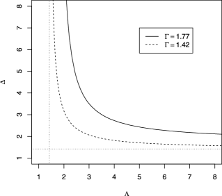
Figure 5: Amplification or re-expression of a sensitivity involving one parameter $\Gamma$ at $\Gamma=1.77$ or $\Gamma=1.42$ into an equivalent sensitivity analysis involving two parameters. Here, $\Lambda$ controls the relationship between treatment assignment, namely $Z_{i1}-Z_{i2}$, and the unobserved covariate, $u_{i1}-u_{i2}$, and $\Delta$ controls the relationship between a positive response difference under ${H}_{0}$, namely $R_{i1}-R_{i2}=r_{Ci1}-r_{Ci2}$, and the unobserved covariate, $u_{i1}-u_{i2}$. For instance, $(\Lambda,\Delta)=(3.00,2.06)$ is equivalent to $\Gamma=1.42$ while $(\Lambda,\Delta)=(3.00,3.50)$ is equivalent to $\Gamma=1.77$. The dotted lines are at the asymptote of 1.42 for $\Gamma=1.42$.

Figure 5 depicts the amplification of the sensitivity analysis in Table 3, so that, as in Section 3.5, the single values of $\Gamma=1.42$ and $\Gamma=1.77$ are expressed as the corresponding curves of $(\Lambda,\Delta)$ at $\Gamma=(\Lambda\Delta+1)/(\Lambda+\Delta)$. In particular, the curve for $\Gamma=1.42$ includes $(\Lambda,\Delta)=(3,2.06)$, or an unobserved covariate $u$ that roughly a triples the odds of treatment and doubles the odds of a positive difference in test scores. In contrast, the $\Gamma=1.77$ includes $(\Lambda,\Delta)=(3,3.50)$, or roughly a tripling of the odds of treatment and a 3.5-fold increase in the odds of a positive difference in test scores. The reduction in heterogeneity in Figure 3 moves the degree of sensitivity from $\Gamma=1.42$ to $\Gamma=1.77$, and for $\Lambda=3$ this is a move from $\Delta\doteq 2$ to $\Delta\doteq 3.5$. In view of this, a meaningful reduction in sensitivity to unmeasured biases was produced by balancing all covariates first in Section 2.2 and closely pairing for the predictive covariates in Section 2.3.

5 Summary

In matching, covariate balance refers to the distributions of the observed covariate $\mathbf{x}$ in treated and control groups. Cardinality matching constructs the largest matched sample that satisfies specified constraints (1) on covariate balance $\mathbf{x}$, ignoring who is paired with whom. With this first task accomplished, with comparable groups in hand, the pairing can then emphasize a subset of covariates expected to predict the outcome and hence to reduce heterogeneity of the treated-minus-control pair differences $Y$. In the example, one pairing used all observed covariates, the other used only pretreatment test scores, with precisely the same students in both pairings, differing only in who was paired with whom. The same size treatment effect with less heterogeneity or dispersion of $Y$ tends to be less sensitive to unmeasured biases, that is, reduced heterogeneity increases the design sensitivity $\widetilde{\Gamma}$; see Section 3.4. In the example, the mean pair difference in $Y$ of 17.5 test score points was meaningfully less sensitive to unmeasured biases when a pairing based on all covariates was replaced by a pairing focused on a few predictive covariates yielding a modest reduction in heterogeneity from a standard deviation of $Y$ of 105.5 to 90.9. As seen in the sequence of sensitivity analyses that began with the conventional match and analysis in the first column of Table 1 and ended with the proposed match and analysis in the last column of Table 3, better matching algorithms that reduce heterogeneity together with better statistical tests yielded a substantial reduction in the reported sensitivity to unmeasured biases. Moreover, as discussed in Section 3, statistical theory suggests this reduction in reported sensitivity to bias is expected to occur when there is an actual treatment effect under simple models for the generation of the data.

Supplement to “Matching for balance, pairing for heterogeneity in an observational study of the effectiveness of for-profit and not-for-profit high schools in Chile” [doi]10.1214/13-AOAS713SUPP .pdf aoas713_supp.pdf In an online supplement we provide additional summary tables for covariate balance.

References

- Angrist, Pathak and Walters (2013) {barticle}[auto:STB—2014/01/06—10:16:28] \bauthor\bsnmAngrist, \bfnmJ. D.\binitsJ. D., \bauthor\bsnmPathak, \bfnmP. A.\binitsP. A. and \bauthor\bsnmWalters, \bfnmC. R.\binitsC. R. (\byear2013). \btitleExplaining charter school effectiveness. \bjournalAm. Econ. J. \bvolume5 \bpages1–27. \bptokimsref\endbibitem
- Baiocchi (2011) {bmisc}[auto] \bauthor\bsnmBaiocchi, \bfnmMike\binitsM. (\byear2011). \bhowpublishedDesigning robust studies using propensity score and prognostic score matching. Chapter 3 in Methodologies for Observational Studies of Health Care Policy. Ph.D. thesis, Dept. Statistics, The Wharton School, Univ. Pennsylvania, Philadelphia, PA. \bptokimsref\endbibitem
- Bellei (2009) {barticle}[auto:STB—2014/01/06—10:16:28] \bauthor\bsnmBellei, \bfnmC.\binitsC. (\byear2009). \btitleDoes lengthening the school day increase students academic achievement? Results from a natural experiment in Chile. \bjournalEcon. Educ. Rev. \bvolume28 \bpages629–640. \bptokimsref\endbibitem
- Brown (1981) {barticle}[mr] \bauthor\bsnmBrown, \bfnmB. M.\binitsB. M. (\byear1981). \btitleSymmetric quantile averages and related estimators. \bjournalBiometrika \bvolume68 \bpages235–242. \biddoi=10.1093/biomet/68.1.235, issn=0006-3444, mr=0614960 \bptokimsref\endbibitem
- Cornfield et al. (1959) {barticle}[auto:STB—2014/01/06—10:16:28] \bauthor\bsnmCornfield, \bfnmJ.\binitsJ., \bauthor\bsnmHaenszel, \bfnmW.\binitsW., \bauthor\bsnmHammond, \bfnmE.\binitsE., \bauthor\bsnmLilienfeld, \bfnmA.\binitsA., \bauthor\bsnmShimkin, \bfnmM.\binitsM. and \bauthor\bsnmWynder, \bfnmE.\binitsE. (\byear1959). \btitleSmoking and lung cancer. \bjournalJ. Natl. Cancer Inst. \bvolume22 \bpages173–203. \bptokimsref\endbibitem
- Cox (1958) {bbook}[mr] \bauthor\bsnmCox, \bfnmD. R.\binitsD. R. (\byear1958). \btitlePlanning of Experiments. \bseriesA Wiley Publication in Applied Statistics. \bpublisherWiley, \blocationNew York. \bidmr=0095561 \bptokimsref\endbibitem
- Crump et al. (2009) {barticle}[mr] \bauthor\bsnmCrump, \bfnmRichard K.\binitsR. K., \bauthor\bsnmHotz, \bfnmV. Joseph\binitsV. J., \bauthor\bsnmImbens, \bfnmGuido W.\binitsG. W. and \bauthor\bsnmMitnik, \bfnmOscar A.\binitsO. A. (\byear2009). \btitleDealing with limited overlap in estimation of average treatment effects. \bjournalBiometrika \bvolume96 \bpages187–199. \biddoi=10.1093/biomet/asn055, issn=0006-3444, mr=2482144 \bptokimsref\endbibitem
- Deyo, Cherkin and Ciol (1992) {barticle}[pbm] \bauthor\bsnmDeyo, \bfnmR. A.\binitsR. A., \bauthor\bsnmCherkin, \bfnmD. C.\binitsD. C. and \bauthor\bsnmCiol, \bfnmM. A.\binitsM. A. (\byear1992). \btitleAdapting a clinical comorbidity index for use with ICD-9-CM administrative databases. \bjournalJ. Clin. Epidemiol. \bvolume45 \bpages613–619. \bidissn=0895-4356, pii=0895-4356(92)90133-8, pmid=1607900 \bptokimsref\endbibitem
- Elacqua (2009) {bmisc}[auto:STB—2014/02/12—14:17:21] \bauthor\bsnmElacqua, \bfnmG.\binitsG. (\byear2009). \bhowpublishedThe Impact of School Choice and Public Policy on Segregation: Evidence from Chile. Centro de Políticas Comparadas de Educación, Univ. Diego Portales, Santiago, Chile. \bptokimsref\endbibitem
- Fisher (1935) {bbook}[auto:STB—2014/01/06—10:16:28] \bauthor\bsnmFisher, \bfnmR. A.\binitsR. A. (\byear1935). \btitleThe Design of Experiments. \bpublisherOliver & Boyd, \blocationEdinburgh. \bptokimsref\endbibitem
- Gastwirth (1992) {barticle}[auto:STB—2014/01/06—10:16:28] \bauthor\bsnmGastwirth, \bfnmJ. L.\binitsJ. L. (\byear1992). \btitleMethods for assessing the sensitivity of statistical comparisons used in Title VII cases to omitted variables. \bjournalJurimetrics \bvolume33 \bpages19–34. \bptokimsref\endbibitem
- Hansen (2007) {barticle}[auto:STB—2014/01/06—10:16:28] \bauthor\bsnmHansen, \bfnmB. B.\binitsB. B. (\byear2007). \btitleOptmatch: Flexible, optimal matching for observational studies. \bjournalR News \bvolume7 \bpages18–24. \bnote(Package optmatch in R). \bptokimsref\endbibitem
- Hansen (2008) {barticle}[mr] \bauthor\bsnmHansen, \bfnmBen B.\binitsB. B. (\byear2008). \btitleThe prognostic analogue of the propensity score. \bjournalBiometrika \bvolume95 \bpages481–488. \biddoi=10.1093/biomet/asn004, issn=0006-3444, mr=2521594 \bptokimsref\endbibitem
- Hill and Su (2013) {barticle}[mr] \bauthor\bsnmHill, \bfnmJennifer\binitsJ. and \bauthor\bsnmSu, \bfnmYu-Sung\binitsY.-S. (\byear2013). \btitleAssessing lack of common support in causal inference using Bayesian nonparametrics: Implications for evaluating the effect of breastfeeding on children’s cognitive outcomes. \bjournalAnn. Appl. Stat. \bvolume7 \bpages1386–1420. \biddoi=10.1214/13-AOAS630, issn=1932-6157, mr=3127952 \bptokimsref\endbibitem
- Hodges and Lehmann (1963) {barticle}[mr] \bauthor\bsnmHodges, \bfnmJ. L.\binitsJ. L. \bsuffixJr. and \bauthor\bsnmLehmann, \bfnmE. L.\binitsE. L. (\byear1963). \btitleEstimates of location based on rank tests. \bjournalAnn. Math. Statist. \bvolume34 \bpages598–611. \bidissn=0003-4851, mr=0152070 \bptokimsref\endbibitem
- Hosman, Hansen and Holland (2010) {barticle}[mr] \bauthor\bsnmHosman, \bfnmCarrie A.\binitsC. A., \bauthor\bsnmHansen, \bfnmBen B.\binitsB. B. and \bauthor\bsnmHolland, \bfnmPaul W.\binitsP. W. (\byear2010). \btitleThe sensitivity of linear regression coefficients’ confidence limits to the omission of a confounder. \bjournalAnn. Appl. Stat. \bvolume4 \bpages849–870. \biddoi=10.1214/09-AOAS315, issn=1932-6157, mr=2758424 \bptokimsref\endbibitem
- Iacus, King and Porro (2009) {barticle}[auto:STB—2014/01/06—10:16:28] \bauthor\bsnmIacus, \bfnmS. M.\binitsS. M., \bauthor\bsnmKing, \bfnmG.\binitsG. and \bauthor\bsnmPorro, \bfnmG.\binitsG. (\byear2009). \btitleSoftware for coarsened exact matching. \bjournalJ. Stat. Softw. \bvolume30 \bpages1–27. \bptokimsref\endbibitem
- Knaus et al. (1985) {barticle}[pbm] \bauthor\bsnmKnaus, \bfnmW. A.\binitsW. A., \bauthor\bsnmDraper, \bfnmE. A.\binitsE. A., \bauthor\bsnmWagner, \bfnmD. P.\binitsD. P. and \bauthor\bsnmZimmerman, \bfnmJ. E.\binitsJ. E. (\byear1985). \btitleAPACHE II: A severity of disease classification system. \bjournalCrit. Care Med. \bvolume13 \bpages818–829. \bidissn=0090-3493, pmid=3928249 \bptokimsref\endbibitem
- Lehmann (1975) {bbook}[auto:STB—2014/01/06—10:16:28] \bauthor\bsnmLehmann, \bfnmE. L.\binitsE. L. (\byear1975). \btitleNonparametrics. \bpublisherHolden-Day, \blocationSan Francisco, CA. \bptokimsref\endbibitem
- Lu et al. (2011) {barticle}[mr] \bauthor\bsnmLu, \bfnmBo\binitsB., \bauthor\bsnmGreevy, \bfnmRobert\binitsR., \bauthor\bsnmXu, \bfnmXinyi\binitsX. and \bauthor\bsnmBeck, \bfnmCole\binitsC. (\byear2011). \btitleOptimal nonbipartite matching and its statistical applications. \bjournalAmer. Statist. \bvolume65 \bpages21–30. \bnote(Package nbpmatching in R). \biddoi=10.1198/tast.2011.08294, issn=0003-1305, mr=2899649 \bptokimsref\endbibitem
- Marcus (1997) {barticle}[auto:STB—2014/01/06—10:16:28] \bauthor\bsnmMarcus, \bfnmS. M.\binitsS. M. (\byear1997). \btitleUsing omitted variable bias to assess uncertainty in the estimation of an AIDS education treatment effect. \bjournalJ. Educ. Statist. \bvolume22 \bpages193–201. \bptokimsref\endbibitem
- Maritz (1979) {barticle}[mr] \bauthor\bsnmMaritz, \bfnmJ. S.\binitsJ. S. (\byear1979). \btitleA note on exact robust confidence intervals for location. \bjournalBiometrika \bvolume66 \bpages163–166. \biddoi=10.1093/biomet/66.1.163, issn=0006-3444, mr=0529161 \bptokimsref\endbibitem
- Neyman (1923) {barticle}[auto] \bauthor\bsnmNeyman, \bfnmJ.\binitsJ. (\byear1923, 1990). \btitleOn the application of probability theory to agricultural experiments. \bjournalStatist. Sci. \bvolume5 \bpages463–480. \bptokimsref\endbibitem
- Rosenbaum (1987) {barticle}[mr] \bauthor\bsnmRosenbaum, \bfnmPaul R.\binitsP. R. (\byear1987). \btitleSensitivity analysis for certain permutation inferences in matched observational studies. \bjournalBiometrika \bvolume74 \bpages13–26. \biddoi=10.1093/biomet/74.1.13, issn=0006-3444, mr=0885915 \bptokimsref\endbibitem
- Rosenbaum (1993) {barticle}[mr] \bauthor\bsnmRosenbaum, \bfnmPaul R.\binitsP. R. (\byear1993). \btitleHodges–Lehmann point estimates of treatment effect in observational studies. \bjournalJ. Amer. Statist. Assoc. \bvolume88 \bpages1250–1253. \bidissn=0162-1459, mr=1245357 \bptokimsref\endbibitem
- Rosenbaum (2002) {bbook}[mr] \bauthor\bsnmRosenbaum, \bfnmPaul R.\binitsP. R. (\byear2002). \btitleObservational Studies, \bedition2nd ed. \bpublisherSpringer, \blocationNew York. \bidmr=1899138 \bptokimsref\endbibitem
- Rosenbaum (2004) {barticle}[mr] \bauthor\bsnmRosenbaum, \bfnmPaul R.\binitsP. R. (\byear2004). \btitleDesign sensitivity in observational studies. \bjournalBiometrika \bvolume91 \bpages153–164. \biddoi=10.1093/biomet/91.1.153, issn=0006-3444, mr=2050466 \bptokimsref\endbibitem
- Rosenbaum (2005) {barticle}[mr] \bauthor\bsnmRosenbaum, \bfnmPaul R.\binitsP. R. (\byear2005). \btitleHeterogeneity and causality: Unit heterogeneity and design sensitivity in observational studies. \bjournalAmer. Statist. \bvolume59 \bpages147–152. \biddoi=10.1198/000313005X42831, issn=0003-1305, mr=2133562 \bptokimsref\endbibitem
- Rosenbaum (2007) {barticle}[mr] \bauthor\bsnmRosenbaum, \bfnmPaul R.\binitsP. R. (\byear2007). \btitleSensitivity analysis for -estimates, tests, and confidence intervals in matched observational studies. \bjournalBiometrics \bvolume63 \bpages456–464. \bnote(R package sensitivitymv). \biddoi=10.1111/j.1541-0420.2006.00717.x, issn=0006-341X, mr=2370804 \bptokimsref\endbibitem
- Rosenbaum (2010a) {bbook}[mr] \bauthor\bsnmRosenbaum, \bfnmPaul R.\binitsP. R. (\byear2010a). \btitleDesign of Observational Studies. \bseriesSpringer Series in Statistics. \bpublisherSpringer, \blocationNew York. \biddoi=10.1007/978-1-4419-1213-8, mr=2561612 \bptokimsref\endbibitem
- Rosenbaum (2010b) {barticle}[mr] \bauthor\bsnmRosenbaum, \bfnmPaul R.\binitsP. R. (\byear2010b). \btitleDesign sensitivity and efficiency in observational studies. \bjournalJ. Amer. Statist. Assoc. \bvolume105 \bpages692–702. \biddoi=10.1198/jasa.2010.tm09570, issn=0162-1459, mr=2724853 \bptokimsref\endbibitem
- Rosenbaum (2011) {barticle}[mr] \bauthor\bsnmRosenbaum, \bfnmPaul R.\binitsP. R. (\byear2011). \btitleA new U-statistic with superior design sensitivity in matched observational studies. \bjournalBiometrics \bvolume67 \bpages1017–1027. \biddoi=10.1111/j.1541-0420.2010.01535.x, issn=0006-341X, mr=2829236 \bptokimsref\endbibitem
- Rosenbaum (2012a) {barticle}[mr] \bauthor\bsnmRosenbaum, \bfnmP. R.\binitsP. R. (\byear2012a). \btitleTesting one hypothesis twice in observational studies. \bjournalBiometrika \bvolume99 \bpages763–774. \biddoi=10.1093/biomet/ass032, issn=0006-3444, mr=2999159 \bptokimsref\endbibitem
- Rosenbaum (2012b) {barticle}[mr] \bauthor\bsnmRosenbaum, \bfnmPaul R.\binitsP. R. (\byear2012b). \btitleOptimal matching of an optimally chosen subset in observational studies. \bjournalJ. Comput. Graph. Statist. \bvolume21 \bpages57–71. \biddoi=10.1198/jcgs.2011.09219, issn=1061-8600, mr=2913356 \bptokimsref\endbibitem
- Rosenbaum (2013) {barticle}[mr] \bauthor\bsnmRosenbaum, \bfnmPaul R.\binitsP. R. (\byear2013). \btitleImpact of multiple matched controls on design sensitivity in observational studies. \bjournalBiometrics \bvolume69 \bpages118–127. \biddoi=10.1111/j.1541-0420.2012.01821.x, issn=0006-341X, mr=3058058 \bptokimsref\endbibitem
- Rosenbaum and Rubin (1983) {barticle}[auto:STB—2014/01/06—10:16:28] \bauthor\bsnmRosenbaum, \bfnmP.\binitsP. and \bauthor\bsnmRubin, \bfnmD.\binitsD. (\byear1983). \btitleAssessing sensitivity to an unobserved binary covariate in an observational study with binary outcome. \bjournalJ. Roy. Statist. Soc. Ser. B \bvolume45 \bpages212–218. \bptokimsref\endbibitem
- Rosenbaum and Silber (2009) {barticle}[mr] \bauthor\bsnmRosenbaum, \bfnmPaul R.\binitsP. R. and \bauthor\bsnmSilber, \bfnmJeffrey H.\binitsJ. H. (\byear2009). \btitleAmplification of sensitivity analysis in matched observational studies. \bjournalJ. Amer. Statist. Assoc. \bvolume104 \bpages1398–1405. \biddoi=10.1198/jasa.2009.tm08470, issn=0162-1459, mr=2750570 \bptokimsref\endbibitem
- Rubin (1974) {barticle}[auto:STB—2014/01/06—10:16:28] \bauthor\bsnmRubin, \bfnmD. B.\binitsD. B. (\byear1974). \btitleEstimating causal effects of treatments in randomized and nonrandomized studies. \bjournalJ. Ed. Psych. \bvolume66 \bpages688–701. \bptokimsref\endbibitem
- Rubin (1979) {barticle}[auto:STB—2014/01/06—10:16:28] \bauthor\bsnmRubin, \bfnmD. B.\binitsD. B. (\byear1979). \btitleUsing multivariate matched sampling and regression adjustment to control bias in observational studies. \bjournalJ. Amer. Statist. Assoc. \bvolume74 \bpages318–328. \bptokimsref\endbibitem
- Small (2007) {barticle}[mr] \bauthor\bsnmSmall, \bfnmDylan S.\binitsD. S. (\byear2007). \btitleSensitivity analysis for instrumental variables regression with overidentifying restrictions. \bjournalJ. Amer. Statist. Assoc. \bvolume102 \bpages1049–1058. \biddoi=10.1198/016214507000000608, issn=0162-1459, mr=2411664 \bptokimsref\endbibitem
- Stephenson (1981) {barticle}[mr] \bauthor\bsnmStephenson, \bfnmW. Robert\binitsW. R. (\byear1981). \btitleA general class of one-sample nonparametric test statistics based on subsamples. \bjournalJ. Amer. Statist. Assoc. \bvolume76 \bpages960–966. \bidissn=0162-1459, mr=0650912 \bptokimsref\endbibitem
- Stuart (2010) {barticle}[mr] \bauthor\bsnmStuart, \bfnmElizabeth A.\binitsE. A. (\byear2010). \btitleMatching methods for causal inference: A review and a look forward. \bjournalStatist. Sci. \bvolume25 \bpages1–21. \biddoi=10.1214/09-STS313, issn=0883-4237, mr=2741812 \bptokimsref\endbibitem
- Traskin and Small (2011) {barticle}[auto:STB—2014/01/06—10:16:28] \bauthor\bsnmTraskin, \bfnmM.\binitsM. and \bauthor\bsnmSmall, \bfnmD. S.\binitsD. S. (\byear2011). \btitleDefining the study population for an observational study to ensure suffient overlap: A tree approach. \bjournalStatist. Biosci. \bvolume3 \bpages94–118. \bptokimsref\endbibitem
- Wang and Krieger (2006) {barticle}[mr] \bauthor\bsnmWang, \bfnmLiansheng\binitsL. and \bauthor\bsnmKrieger, \bfnmAbba M.\binitsA. M. (\byear2006). \btitleCausal conclusions are most sensitive to unobserved binary covariates. \bjournalStat. Med. \bvolume25 \bpages2257–2271. \biddoi=10.1002/sim.2344, issn=0277-6715, mr=2240099 \bptokimsref\endbibitem
- Welch (1937) {barticle}[auto:STB—2014/01/06—10:16:28] \bauthor\bsnmWelch, \bfnmB. L.\binitsB. L. (\byear1937). \btitleOn the -test in randomized blocks. \bjournalBiometrika \bvolume29 \bpages21–52. \bptokimsref\endbibitem
- Wolfe (1974) {barticle}[mr] \bauthor\bsnmWolfe, \bfnmDouglas A.\binitsD. A. (\byear1974). \btitleA characterization of population weighted-symmetry and related results. \bjournalJ. Amer. Statist. Assoc. \bvolume69 \bpages819–822. \bidissn=0162-1459, mr=0426239 \bptokimsref\endbibitem
- Yanagawa (1984) {barticle}[mr] \bauthor\bsnmYanagawa, \bfnmTakashi\binitsT. (\byear1984). \btitleCase–control studies: Assessing the effect of a confounding factor. \bjournalBiometrika \bvolume71 \bpages191–194. \biddoi=10.1093/biomet/71.1.191, issn=0006-3444, mr=0738341 \bptokimsref\endbibitem
- Yang et al. (2012) {barticle}[mr] \bauthor\bsnmYang, \bfnmDan\binitsD., \bauthor\bsnmSmall, \bfnmDylan S.\binitsD. S., \bauthor\bsnmSilber, \bfnmJeffrey H.\binitsJ. H. and \bauthor\bsnmRosenbaum, \bfnmPaul R.\binitsP. R. (\byear2012). \btitleOptimal matching with minimal deviation from fine balance in a study of obesity and surgical outcomes. \bjournalBiometrics \bvolume68 \bpages628–636. \bnote(R package finebalance). \biddoi=10.1111/j.1541-0420.2011.01691.x, issn=0006-341X, mr=2959630 \bptokimsref\endbibitem
- Yu and Gastwirth (2005) {barticle}[auto:STB—2014/01/06—10:16:28] \bauthor\bsnmYu, \bfnmB. B.\binitsB. B. and \bauthor\bsnmGastwirth, \bfnmJ. L.\binitsJ. L. (\byear2005). \btitleSensitivity analysis for trend tests: Application to the risk of radiation exposure. \bjournalBiostatistics \bvolume6 \bpages201–209. \bptokimsref\endbibitem
- Zubizarreta (2012) {barticle}[mr] \bauthor\bsnmZubizarreta, \bfnmJosé R.\binitsJ. R. (\byear2012). \btitleUsing mixed integer programming for matching in an observational study of kidney failure after surgery. \bjournalJ. Amer. Statist. Assoc. \bvolume107 \bpages1360–1371. \bnote(R software mipmatch at http://www-stat.wharton.upenn.edu/~josezubi/). \biddoi=10.1080/01621459.2012.703874, issn=0162-1459, mr=3036400 \bptokimsref\endbibitem
- Zubizarreta, Paredes and Rosenbaum (2014) {bmisc}[auto:STB—2014/01/06—10:16:28] \bauthor\bsnmZubizarreta, \bfnmJosé R.\binitsJ. R., \bauthor\bsnmParedes, \bfnmRicardo D.\binitsR. D. and \bauthor\bsnmRosenbaum, \bfnmPaul R.\binitsP. R. (\byear2014). \bhowpublishedSupplement to: “Matching for balance, pairing for heterogeneity in an observational study of the effectiveness of for-profit and not-for-profit high schools in Chile.” DOI:\doiurl10.1214/13-AOAS713SUPP. \bptokimsref \endbibitem
- Zubizarreta et al. (2011) {barticle}[mr] \bauthor\bsnmZubizarreta, \bfnmJosé R.\binitsJ. R., \bauthor\bsnmReinke, \bfnmCaroline E.\binitsC. E., \bauthor\bsnmKelz, \bfnmRachel R.\binitsR. R., \bauthor\bsnmSilber, \bfnmJeffrey H.\binitsJ. H. and \bauthor\bsnmRosenbaum, \bfnmPaul R.\binitsP. R. (\byear2011). \btitleMatching for several sparse nominal variables in a case–control study of readmission following surgery. \bjournalAmer. Statist. \bvolume65 \bpages229–238. \biddoi=10.1198/tas.2011.11072, issn=0003-1305, mr=2867507 \bptokimsref\endbibitem