Random forests with random projections of the output space for high dimensional multi-label classification

Abstract

We adapt the idea of random projections applied to the output space, so as to enhance tree-based ensemble methods in the context of multi-label classification. We show how learning time complexity can be reduced without affecting computational complexity and accuracy of predictions. We also show that random output space projections may be used in order to reach different bias-variance tradeoffs, over a broad panel of benchmark problems, and that this may lead to improved accuracy while reducing significantly the computational burden of the learning stage.

1 Introduction

Within supervised learning, the goal of multi-label classification is to train models to annotate objects with a subset of labels taken from a set of candidate labels. Typical applications include the determination of topics addressed in a text document, the identification of object categories present within an image, or the prediction of biological properties of a gene. In many applications, the number of candidate labels may be very large, ranging from hundreds to hundreds of thousands [2] and often even exceeding the sample size [12]. The very large scale nature of the output space in such problems poses both statistical and computational challenges that need to be specifically addressed.

A simple approach to solve multi-label classification problems, called binary relevance, is to train independently a binary classifier for each label. Several more complex schemes have however been proposed to take into account the dependencies between the labels (see, e.g. [28, 19, 9, 33, 10, 39]). In the context of tree-based methods, one way is to train multi-output trees [4, 18, 23], ie. trees that can predict multiple outputs at once. With respect to single-output trees [7], the score measure used in multi-output trees to choose splits is taken as the sum of the individual scores corresponding to the different labels (e.g., variance reduction) and each leaf is labeled with a vector of values, coding each for the probability of presence of one label. With respect to binary relevance, the multi-output tree approach has the advantage of building a single model for all labels. It can thus potentially take into account label dependencies and reduce memory requirements for the storage of the models. An extensive experimental comparison [25] shows that this approach compares favorably with other approaches, including non tree-based methods, both in terms of accuracy and computing times. In addition, multi-output trees inherit all intrinsic advantages of tree-based methods, such as robustness to irrelevant features, interpretability through feature importance scores, or fast computations of predictions, that make them very attractive to address multi-label problems. The computational complexity of learning multi-output trees is however similar to that of the binary relevance method. Both approaches are indeed $O(pdn\log n)$, where $p$ is the number of input features, $d$ the number of candidate output labels, and $n$ the sample size; this is a limiting factor when dealing with large sets of candidate labels.

One generic approach to reduce computational complexity is to apply some compression technique prior to the training stage to reduce the number of outputs to a number $m$ much smaller than the total number $d$ of labels. A model can then be trained to make predictions in the compressed output space and a prediction in the original label space can be obtained by decoding the compressed prediction. As multi-label vectors are typically very sparse, one can expect a drastic dimensionality reduction by using appropriate compression techniques. This idea has been explored for example in [19] using compressed sensing,  and in [10] using bloom filters, in both cases using regularized linear models as base learners. This approach obviously reduces computing times for training the model. At the prediction stage however, the predicted compressed output needs to be decoded, which adds computational cost and can also introduce further decoding errors.

In this paper, we explore the use of random output space projections for large-scale multi-label classification in the context of tree-based ensemble methods. We first explore the idea proposed for linear models in [19] with random forests: a (single) random projection of the multi-label vector to an $m$-dimensional random subspace is computed and then a multi-output random forest is grown based on score computations using the projected outputs. We exploit however the fact that the approximation provided by a tree ensemble is a weighted average of output vectors from the training sample to avoid the decoding stage: at training time all leaf labels are directly computed in the original multi-label space. We show theoretically and empirically that when $m$ is large enough, ensembles grown on such random output spaces are equivalent to ensembles grown on the original output space. When $d$ is large enough compared to $n$, this idea hence may reduce computing times at the learning stage without affecting accuracy and computational complexity of predictions.

Next, we propose to exploit the randomization inherent to the projection of the output space as a way to obtain randomized trees in the context of ensemble methods: each tree in the ensemble is thus grown from a different randomly projected subspace of dimension $m$. As previously, labels at leaf nodes are directly computed in the original output space to avoid the decoding step. We show, theoretically, that this idea can lead to better accuracy than the first idea and, empirically, that best results are obtained on many problems with very low values of $m$, which leads to significant computing time reductions at the learning stage. In addition, we study the interaction between input randomization (à la Random Forests) and output randomization (through random projections), showing that there is an interest, both in terms of predictive performance and in terms of computing times, to optimally combine these two ways of randomization. All in all, the proposed approach constitutes a very attractive way to address large-scale multi-label problems with tree-based ensemble methods.

The rest of the paper is structured as follows: Section 2 reviews properties of multi-output tree ensembles and of random projections; Section 3 presents the proposed algorithms and their theoretical properties; Section 4 provides the empirical validations, whereas Section 5 discusses our work and provides further research directions.

2 Background

We denote by $\mathcal{X}$ an input space, and by $\mathcal{Y}$ an output space; without loss of generality, we suppose that $\mathcal{X}=\mathbb{R}^{p}$ (where $p$ denotes the number of input features), and that $\mathcal{Y}=\mathbb{R}^{d}$ (where $d$ is the dimension of the output space). We denote by $P_{{\cal X},{\cal Y}}$ the joint (unknown) sampling density over $\mathcal{X}\times\mathcal{Y}$.

Given a learning sample $\left((x^{i},y^{i})\in(\mathcal{X}\times\mathcal{Y})\right)_{i=1}^{n}$ of $n$ observations in the form of input-output pairs, a supervised learning task is defined as searching for a function $f^{*}:\mathcal{X}\rightarrow\mathcal{Y}$ in a hypothesis space $\mathcal{H}\subset\mathcal{Y}^{\mathcal{X}}$ that minimizes the expectation of some loss function $\ell:\mathcal{Y}\times\mathcal{Y}\rightarrow\mathbb{R}$ over the joint distribution of input / output pairs: $f^{*}\in\arg\min_{f\in\mathcal{H}}E_{P_{{\cal X},{\cal Y}}}\left\{\ell(f(x),y)\right\}.$

NOTATIONS: Superscript indices ($x^{i},y^{i}$) denote (input, output) vectors of an observation $i\in\{1,\ldots,n\}$. Subscript indices (e.g. $x_{j},y_{k}$) denote components of vectors.

2.1 Multi-output tree ensembles

A classification or a regression tree [7] is built using all the input-output pairs as follows: for each node at which the subsample size is greater or equal to a pre-pruning parameter $n_{\min}$, the best split is chosen among the $p$ input features combined with the selection of an optimal cut point. The best sample split $(S_{r},S_{l})$ of the local subsample $S$ minimizes the average reduction of impurity

$$\Delta I((y^{i})_{i\in S},(y^{i})_{i\in S_{l}},(y^{i})_{i\in S_{r}})= I((y^{i})_{i\in S})-\frac{|S_{l}|}{|S|}I((y^{i})_{i\in S_{l}})-\frac{|S_{r}|}{|S|}I((y^{i})_{i\in S_{r}}).$$ (1)

Finally, leaf statistics are obtained by aggregating the outputs of the samples reaching that leaf.

In this paper, for multi-output trees, we use the sum of the variances of the $d$ dimensions of the output vector as an impurity measure. It can be computed by (see Appendix A, in the supplementary material)

$$\operatorname{Var}((y^{i})_{i\in S}) =\frac{1}{|S|}\sum_{i\in S}||y^{i}-\frac{1}{|S|}\sum_{i\in S}y^{i}||^{2},$$ (2)

$$=\frac{1}{2|S|^{2}}\sum_{i\in S}\sum_{j\in S}||y^{i}-y^{j}||^{2}.$$ (3)

Furthermore, we compute the vectors of output statistics by component-wise averaging. Notice that, when the outputs are vectors of binary class-labels (i.e. $y\in\{0,1\}^{d}$), as in multi-label classification, the variance reduces to the so-called Gini-index, and the leaf statistics then estimate a vector of conditional probabilities $P(y_{j}=1|x\in leaf)$, from which a prediction $\hat{y}$ can be made by thresholding.

Tree-based ensemble methods build an ensemble of $t$ randomized trees. Unseen samples are then predicted by aggregating the predictions of all $t$ trees. Random Forests [6] build each tree on a bootstrap copy of the learning sample [6] and by optimising the split at each node over a locally generated random subset of size $k$ among the $p$ input features. Extra Trees [17] use the complete learning sample and optimize the split over a random subset of size $k$ of the $p$ features combined with a random selection of cut points. Setting the parameter $k$ to the number of input features $p$ allows to filter out irrelevant features; larger $n_{\min}$ yields simpler trees possibly at the price of higher bias, and the higher $t$ the smaller the variance of the resulting predictor.

2.2 Random projections

In this paper we apply the idea of random projections to samples of vectors of the output space $\mathcal{Y}$. With this in mind, we recall the Johnson-Lindenstrauss lemma (reduced to linear maps), while using our notations.

Lemma 1

Johnson-Lindenstrauss lemma [20] Given $\epsilon>0$ and an integer $n$, let $m$ be a positive integer such that $m\geq 8\epsilon^{-2}\ln{n}$. For any sample $(y^{i})_{i=1}^{n}$ of $n$ points in $\mathbb{R}^{d}$ there exists a matrix $\Phi\in\mathbb{R}^{m\times d}$ such that for all $i,j\in\{1,\ldots,n\}$

$$(1-\epsilon)||y^{i}-y^{j}||^{2}\leq||\Phi y^{i}-\Phi y^{j}||^{2}\leq(1+\epsilon)||y^{i}-y^{j}||^{2}.$$ (4)

Moreover, when $d$ is sufficiently large, several random matrices satisfy (4) with high probability. In particular, we can consider Gaussian matrices which elements are drawn i.i.d. in $\mathcal{N}(0,1/m)$, as well as (sparse) Rademacher matrices which elements are drawn in $\left\{-\sqrt{\frac{s}{m}},0,\sqrt{\frac{s}{m}}\right\}$ with probability $\left\{\frac{1}{2s},1-\frac{1}{s},\frac{1}{2s}\right\}$, where $1/s\in(0,1]$ controls the sparsity of $\Phi$ [1, 24].

Notice that if some $\Phi$ satisfies (4) for the whole learning sample, it obviously satisfies (4) for any subsample that could reach a node during regression tree growing. On the other hand, since we are not concerned in this paper with the ‘reconstruction’ problem, we do not need to make any sparsity assumption ‘à la compressed sensing’.

3 Methods

We first present how we propose to exploit random projections to reduce the computational burden of learning single multi-output trees in very high-dimensional output spaces. Then we present and compare two ways to exploit this idea with ensembles of trees. Subsection  3.3 analyses these two ways from the bias/variance point of view.

3.1 Multi-output regression trees in randomly projected output spaces

The multi-output single tree algorithm described in section 2 requires the computation of the sum of variances in (2) at each tree node and for each candidate split. When $\mathcal{Y}$ is very high-dimensional, this computation constitutes the main computational bottleneck of the algorithm. We thus propose to approximate variance computations by using random projections of the output space. The multi-output regression tree algorithm is modified as follows (denoting by $LS$ the learning sample $((x^{i},y^{i}))_{i=1}^{n}$):

• First, a projection matrix $\Phi$ of dimension $m\times d$ is randomly generated.

• A new dataset $LS_{m}=((x^{i},\Phi y^{i}))_{i=1}^{n}$ is constructed by projecting each learning sample output using the projection matrix $\Phi$.

• A tree (structure) $\cal T$ is grown using the projected learning sample $LS_{m}$.

• Predictions $\hat{y}$ at each leaf of $\cal T$ are computed using the corresponding outputs in the original output space.

The resulting tree is exploited in the standard way to make predictions: an input vector $x$ is propagated through the tree until it reaches a leaf from which a prediction $\hat{y}$ in the original output space is directly retrieved.

If $\Phi$ satisfies (4), the following theorem shows that variance computed in the projected subspace is an $\epsilon$-approximation of the variance computed over the original space.

Theorem 3.1

Given $\epsilon>0$, a sample $(y^{i})_{i=1}^{n}$ of $n$ points $y\in\mathbb{R}^{d}$, and a projection matrix $\Phi\in\mathbb{R}^{m\times d}$ such that for all $i,j\in\{1,\ldots,n\}$ condition (4) holds, we have also:

$$(1-\epsilon)\operatorname{Var}((y^{i})_{i=1}^{n})\leq\operatorname{Var}((\Phi y^{i})_{i=1}^{n})\leq(1+\epsilon)\operatorname{Var}((y^{i})_{i=1}^{n}).$$ (5)

Proof

See Appendix B, supplementary material.

As a consequence, any split score approximated from the randomly projected output space will be $\epsilon$-close to the unprojected scores in any subsample of the complete learning sample. Thus, if condition (4) is satisfied for a sufficiently small $\epsilon$ then the tree grown from the projected data will be identical to the tree grown from the original data.

For a given size $m$ of the projection subspace, the complexity is reduced from $O(dn)$ to $O(mn)$ for the computation of one split score and thus from $O(dpn\log n)$ to $O(mpn\log n)$ for the construction of one full (balanced) tree, where one can expect $m$ to be much smaller than $d$ and at worst of $O(\epsilon^{-2}\log{n})$. The whole procedure requires to generate the projection matrix and to project the training data. These two steps are respectively $O(dm)$ and $O(ndm)$ but they can often be significantly accelerated by exploiting the sparsity of the projection matrix and/or of the original output data, and they are called only once before growing the tree.

All in all, this means that when $d$ is sufficiently large, the random projection approach may allow us to significantly reduce tree building complexity from $O(dtpn\log n)$ to $O(mtpn~\log n+tndm)$, without impact on predictive accuracy (see section 4, for empirical results).

3.2 Exploitation in the context of tree ensembles

The idea developed in the previous section can be directly exploited in the context of ensembles of randomized multi-output regression trees. Instead of building a single tree from the projected learning sample $LS_{m}$, one can grow a randomized ensemble of them. This “shared subspace” algorithm is described in pseudo-code in Algorithm 1.

Algorithm 1 Tree ensemble on a single shared subspace $\Phi$

0:  $t$, the ensemble size

0:  $((x^{i},y^{i})\in(\mathbb{R}^{p}\times\mathbb{R}^{d}))_{i=1}^{n}$, the input-output pairs

0:  A tree building algorithm.

0:  A sub-space generator

  Generate a sub-space $\Phi\in\mathbb{R}^{m\times d}$;

  for $j=1$ to $t$ do

     Build a tree structure $\mathcal{T}_{j}$ using $((x^{i},\Phi y^{i}))_{i=1}^{n}$;

     Label the leaves of $\mathcal{T}_{j}$ using $((x^{i},y^{i}))_{i=1}^{n}$;

     Add the labelled tree $\mathcal{T}_{j}$ to the ensemble;

  end for

Another idea is to exploit the random projections used so as to introduce a novel kind of diversity among the different trees of an ensemble. Instead of building all the trees of the ensemble from a same shared output-space projection, one could instead grow each tree in the ensemble from a different output-space projection. Algorithm 2 implements this idea in pseudo-code. The randomization introduced by the output space projection can of course be combined with any existing randomization scheme to grow ensembles of trees. In this paper, we will consider the combination of random projections with the randomizations already introduced in Random Forests and Extra Trees. The interplay between these different randomizations will be discussed theoretically in the next subsection by a bias/variance analysis and empirically in Section 4. Note that while when looking at single trees or shared ensembles, the size $m$ of the projected subspace should not be too small so that condition (4) is satisfied, the optimal value of $m$ when projections are randomized at each tree is likely to be smaller, as suggested by the bias/variance analysis in the next subsection.

Algorithm 2 Tree ensemble with individual subspaces $\Phi_{j}$

0:  $t$, the ensemble size

0:  $((x^{i},y^{i})\in(\mathbb{R}^{p}\times\mathbb{R}^{d}))_{i=1}^{n}$, the input-output pairs

0:  A tree building algorithm.

0:  A sub-space generator

  for $j=1$ to $t$ do

     Generate a sub-space $\Phi_{j}\in\mathbb{R}^{m\times d}$;

     Build a tree structure $\mathcal{T}_{j}$ using $((x^{i},\Phi_{j}y^{i}))_{i=1}^{n}$;

     Label the leaves of $\mathcal{T}_{j}$ using $((x^{i},y^{i}))_{i=1}^{n}$;

     Add the labelled tree $\mathcal{T}_{j}$ to the ensemble;

  end for

From the computational point of view, the main difference between these two ways of transposing random-output projections to ensembles of trees is that in the case of Algorithm 2, the generation of the projection matrix $\Phi$ and the computation of projected outputs is carried out $t$ times, while it is done only once for the case of Algorithm 1. These aspects will be empirically evaluated in Section 4.

3.3 Bias/variance analysis

In this subsection, we adapt the bias/variance analysis carried out in [17] to take into account random output projections. The details of the derivations are reported in Appendix C (supplementary material).

Let us denote by $f(.;ls,\phi,\epsilon):{\cal X}\rightarrow\mathbb{R}^{d}$ a single multi-output tree obtained from a projection matrix $\phi$ (below we use $\Phi$ to denote the corresponding random variable), where $\epsilon$ is the value of a random variable $\varepsilon$ capturing the random perturbation scheme used to build this tree (e.g., bootstrapping and/or random input space selection). The square error of this model at some point $x\in{\cal X}$ is defined by:

$$Err(f(x;ls,\phi,\epsilon))\stackrel{{\scriptstyle\text{def}}}{{=}}E_{Y|x}\{||Y-f(x;ls,\phi,\epsilon\})||^{2}\},$$

and its average can decomposed in its residual error, (squared) bias, and variance terms denoted:

$$E_{LS,\Phi,\varepsilon}\{Err(f(x;LS,\Phi,\varepsilon))\}=\sigma^{2}_{R}(x)+B^{2}(x)+V(x)$$

where the variance term $V(x)$ can be further decomposed as the sum of the following three terms:

$$V_{LS}(x) = \operatorname{Var}_{LS}\{E_{\Phi,\varepsilon|LS}\{f(x;LS,\Phi,\varepsilon)\}\}$$

$$V_{Algo}(x) = E_{LS}\{E_{\Phi|LS}\{\operatorname{Var}_{\varepsilon|LS,\Phi}\{f(x;LS,\Phi,\varepsilon)\}\}\},$$

$$V_{Proj}(x) = E_{LS}\{\operatorname{Var}_{\Phi|LS}\{E_{\varepsilon|LS,\Phi}\{f(x;LS,\Phi,\varepsilon)\}\}\},$$

that measure errors due to the randomness of, respectively, the learning sample, the tree algorithm, and the output space projection (Appendix C, supplementary material).

Approximations computed respectively by algorithms 1 and 2 take the following forms:

• $f_{1}(x;ls,\epsilon^{t},\phi)=\frac{1}{t}\sum_{i=1}^{t}f(x;ls,\phi,\epsilon_{i})$

• $f_{2}(x;ls,\epsilon^{t},\phi^{t})=\frac{1}{t}\sum_{i=1}^{t}f(x;ls,\phi_{i},\epsilon_{i}),$

where $\epsilon^{t}=(\epsilon_{1},\ldots,\epsilon_{t})$ and $\phi^{t}=(\phi_{1},\ldots,\phi_{t})$ are vectors of i.i.d. values of the random variables $\varepsilon$ and $\Phi$ respectively.

We are interested in comparing the average errors of these two algorithms, where the average is taken over all random parameters (including the learning sample). We show (Appendix C) that these can be decomposed as follows:

$$E_{LS,\Phi,\varepsilon^{t}}\{Err(f_{1}(x;LS,\Phi,\varepsilon^{t}))\}$$

$$=\sigma^{2}_{R}(x)+B^{2}(x)+V_{LS}(x)+\frac{V_{Algo}(x)}{t}+V_{Proj}(x),$$

$$E_{LS,\Phi^{t},\varepsilon^{t}}\{Err(f_{2}(x;LS,\Phi^{t},\varepsilon^{t}))\}$$

$$=\sigma^{2}_{R}(x)+B^{2}(x)+V_{LS}(x)+\frac{V_{Algo}(x)+V_{Proj}(x)}{t}.$$

From this result, it is hence clear that Algorithm 2 can not be worse, on the average, than Algorithm 1. If the additional computational burden needed to generate a different random projection for each tree is not problematic, then Algorithm 2 should always be preferred to Algorithm 1.

For a fixed level of tree randomization ($\varepsilon$), whether the additional randomization brought by random projections could be beneficial in terms of predictive performance remains an open question that will be addressed empirically in the next section. Nevertheless, with respect to an ensemble grown from the original output space, one can expect that the output-projections will always increase the bias term, since they disturb the algorithm in its objective of reducing the errors on the learning sample. For small values of $m$, the average error will therefore decrease (with a sufficiently large number $t$ of trees) only if the increase in bias is compensated by a decrease of variance.

The value of $m$, the dimension of the projected subspace, that will lead to the best tradeoff between bias and variance will hence depend both on the level of tree randomization and on the learning problem. The more (resp. less) tree randomization, the higher (resp. the lower) could be the optimal value of $m$, since both randomizations affect bias and variance in the same direction.

4 Experiments

4.1 Accuracy assessment protocol

We assess the accuracy of the predictors for multi-label classification on a test sample (TS) by the “Label Ranking Average Precision (LRAP)” [25], expressed by

$$\text{LRAP}(\hat{f})=\frac{1}{|TS|}\sum_{i\in TS}\frac{1}{|y^{i}|}\sum_{j\in\{k:y^{i}_{k}=1\}}\frac{|\mathcal{L}_{j}^{i}(y^{i})|}{|\mathcal{L}_{j}^{i}(1_{d})|},$$ (6)

where $\hat{f}(x^{i})_{j}$ is the probability (or the score) associated to the label $j$ by the learnt model $\hat{f}$ applied to $x^{i}$, $1_{d}$ is a $d$-dimensional row vector of ones, and

$$\mathcal{L}^{i}_{j}(q)=\left\{k:q_{k}=1\mbox{\leavevmode\nobreak\ and\leavevmode\nobreak\ }\hat{f}(x^{i})_{k}\geq\hat{f}(x^{i})_{j}\right\}.$$

Test samples without any relevant labels (i.e. with $|y^{i}|=0$) were discarded prior to computing the average precision. The best possible average precision is thus 1. Notice that we use indifferently the notation $|\cdot|$ to express the cardinality of a set or the $1$-norm of a vector.

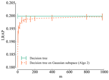
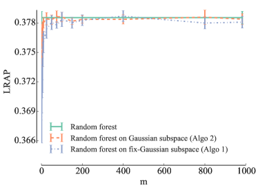
Figure 1: Models built for the “Delicious” dataset ($d=983$) for growing numbers $m$ of Gaussian projections. Left: single unpruned CART trees ($n_{\min}=1$); Right: Random Forests ($k=\sqrt{p}$, $t=100$, $n_{\min}=1$). The curves represent average values (and standard deviations) obtained from 10 applications of the randomised algorithms over a same single $LS/TS$ split.

Table 1: High output space compression ratio is possible, with no or negligible average precision reduction ($t=100$, $n_{\min}=1$, $k=\sqrt{p}$). Each dataset has $n_{LS}$ training samples, $n_{TS}$ testing samples, $p$ input features and $d$ labels. Label ranking average precisions are displayed in terms of their mean values and standard deviations over 10 random $LS/TS$ splits, or over the 10 folds of cross-validation. Mean scores in the last three columns are underlined if they show a difference with respect to the standard Random Forests of more than one standard deviation.

Datasets					Random		Random Forests on Gaussian sub-space
Name	$n_{LS}$	$n_{TS}$	$p$	$d$	Forests		$m=1$		$m=\lfloor 0.5+\ln{d}\rfloor$		$m=d$
emotions	391	202	72	6	$0.800$	$\pm 0.014$	$0.800$	$\pm 0.010$	$0.810$	$\pm 0.014$	$0.810$	$\pm 0.016$
scene	1211	1196	2407	6	$0.870$	$\pm 0.003$	$0.875$	$\pm 0.007$	$0.872$	$\pm 0.004$	$0.872$	$\pm 0.004$
yeast	1500	917	103	14	$0.759$	$\pm 0.008$	$0.748$	$\pm 0.006$	$0.755$	$\pm 0.004$	$0.758$	$\pm 0.005$
tmc2017	21519	7077	49060	22	$0.756$	$\pm 0.003$	$0.741$	$\pm 0.003$	$0.748$	$\pm 0.003$	$0.757$	$\pm 0.003$
genbase	463	199	1186	27	$0.992$	$\pm 0.004$	$0.994$	$\pm 0.002$	$0.994$	$\pm 0.004$	$0.993$	$\pm 0.004$
reuters	2500	5000	19769	34	$0.865$	$\pm 0.004$	$0.864$	$\pm 0.003$	$0.863$	$\pm 0.004$	$0.862$	$\pm 0.004$
medical	333	645	1449	45	$0.848$	$\pm 0.009$	$0.836$	$\pm 0.011$	$0.842$	$\pm 0.014$	$0.841$	$\pm 0.009$
enron	1123	579	1001	53	$0.683$	$\pm 0.009$	$0.680$	$\pm 0.006$	$0.685$	$\pm 0.009$	$0.686$	$\pm 0.008$
mediamill	30993	12914	120	101	$0.779$	$\pm 0.001$	$0.772$	$\pm 0.001$	$0.777$	$\pm 0.002$	$0.779$	$\pm 0.002$
Yeast-GO	2310	1155	5930	132	$0.420$	$\pm 0.010$	$0.353$	$\pm 0.008$	$0.381$	$\pm 0.005$	$0.420$	$\pm 0.010$
bibtex	4880	2515	1836	159	$0.566$	$\pm 0.004$	$0.513$	$\pm 0.006$	$0.548$	$\pm 0.007$	$0.564$	$\pm 0.008$
CAL500	376	126	68	174	$0.504$	$\pm 0.011$	$0.504$	$\pm 0.004$	$0.506$	$\pm 0.007$	$0.502$	$\pm 0.010$
WIPO	1352	358	74435	188	$0.490$	$\pm 0.010$	$0.430$	$\pm 0.010$	$0.460$	$\pm 0.010$	$0.480$	$\pm 0.010$
EUR-Lex (subj.)	19348	10-cv	5000	201	$0.840$	$\pm 0.005$	$0.814$	$\pm 0.004$	$0.828$	$\pm 0.005$	$0.840$	$\pm 0.004$
bookmarks	65892	21964	2150	208	$0.453$	$\pm 0.001$	$0.436$	$\pm 0.002$	$0.445$	$\pm 0.002$	$0.453$	$\pm 0.002$
diatoms	2065	1054	371	359	$0.700$	$\pm 0.010$	$0.650$	$\pm 0.010$	$0.670$	$\pm 0.010$	$0.710$	$\pm 0.020$
corel5k	4500	500	499	374	$0.303$	$\pm 0.012$	$0.309$	$\pm 0.011$	$0.307$	$\pm 0.011$	$0.299$	$\pm 0.013$
EUR-Lex (dir.)	19348	10-cv	5000	412	$0.814$	$\pm 0.006$	$0.782$	$\pm 0.008$	$0.796$	$\pm 0.009$	$0.813$	$\pm 0.007$
SCOP-GO	6507	3336	2003	465	$0.811$	$\pm 0.004$	$0.808$	$\pm 0.005$	$0.811$	$\pm 0.004$	$0.806$	$\pm 0.004$
delicious	12920	3185	500	983	$0.384$	$\pm 0.004$	$0.381$	$\pm 0.003$	$0.382$	$\pm 0.002$	$0.383$	$\pm 0.004$
drug-interaction	1396	466	660	1554	$0.379$	$\pm 0.014$	$0.384$	$\pm 0.009$	$0.378$	$\pm 0.013$	$0.367$	$\pm 0.016$
protein-interaction	1165	389	876	1862	$0.330$	$\pm 0.015$	$0.337$	$\pm 0.016$	$0.337$	$\pm 0.017$	$0.335$	$\pm 0.014$
Expression-GO	2485	551	1288	2717	$0.235$	$\pm 0.005$	$0.211$	$\pm 0.005$	$0.219$	$\pm 0.005$	$0.232$	$\pm 0.005$
EUR-Lex (desc.)	19348	10-cv	5000	3993	$0.523$	$\pm 0.008$	$0.485$	$\pm 0.008$	$0.497$	$\pm 0.009$	$0.523$	$\pm 0.007$

4.2 Effect of the size $m$ of the Gaussian output space

To illustrate the behaviour of our algorithms, we first focus on the “Delicious” dataset [32], which has a large number of labels ($d=983$), of input features ($p=500$), and of training ($n_{LS}=12920$) and testing ($n_{TS}=3185$) samples.

The left part of figure 1 shows, when Gaussian output-space projections are combined with the standard CART algorithm building a single tree, how the precision converges (cf Theorem 3.1) when $m$ increases towards $d$. We observe that in this case, convergence is reached around $m=200$ at the expense of a slight decrease of accuracy, so that a compression factor of about 5 is possible with respect to the original output dimension $d=983$.

The right part of figure 1 shows, on the same dataset, how the method behaves when combined with Random Forests. Let us first notice that the Random Forests grown on the original output space (green line) are significantly more accurate than the single trees, their accuracy being almost twice as high. We also observe that Algorithm 2 (orange curve) converges much more rapidly than Algorithm 1 (blue curve) and slightly outperforms the Random Forest grown on the original output space. It needs only about $m=25$ components to converge, while Algorithm 1 needs about $m=75$ of them. These results are in accordance with the analysis of Section 3.3, showing that Algorithm 2 can’t be inferior to Algorithm 1. In the rest of this paper we will therefore focus on Algorithm 2.

4.3 Systematic analysis over 24 datasets

To assess our methods, we have collected 24 different multi-label classification datasets from the literature (see Section D of the supplementary material, for more information and bibliographic references to these datasets) covering a broad spectrum of application domains and ranges of the output dimension ($d\in[6;3993]$, see Table 1). For 21 of the datasets, we made experiments where the dataset is split randomly into a learning set of size $n_{LS}$, and a test set of size $n_{TS}$, and are repeated 10 times (to get average precisions and standard deviations), and for 3 of them we used a ten-fold cross-validation scheme (see Table 1).

Table 1 shows our results on the 24 multi-label datasets, by comparing Random Forests learnt on the original output space with those learnt by Algorithm 2 combined with Gaussian subspaces of size $m\in\left\{1,d,\ln{d}\right\}$. In these experiments, the three parameters of Random Forests are set respectively to $k=\sqrt{p}$, $n_{\min}=1$ (default values, see [17]) and $t=100$ (reasonable computing budget). Each model is learnt ten times on a different shuffled train/testing split, except for the 3 EUR-lex datasets where we kept the original 10 folds of cross-validation.

We observe that for all datasets (except maybe SCOP-GO), taking $m=d$ leads to a similar average precision to the standard Random Forests, i.e. no difference superior to one standard deviation of the error. On 11 datasets, we see that $m=1$ already yields a similar average precision (values not underlined in column $m=1$). For the 13 remaining datasets, increasing $m$ to $\ln{d}$ significantly decreases the gap with the Random Forest baseline and 3 more datasets reach this baseline. We also observe that on several datasets such as “Drug-interaction” and “SCOP-GO”, better performance on the Gaussian subspace is attained with high output randomization ($m=\left\{1,\ln{d}\right\}$) than with $m=d$. We thus conclude that the optimal level of output randomization (i.e. the optimal value of the ratio $m/d$) which maximizes accuracy performances, is dataset dependent.

While our method is intended for tasks with very high dimensional output spaces, we however notice that even with relatively small numbers of labels, its accuracy remains comparable to the baseline, with suitable $m$.

To complete the analysis, Appendix F considers the same experiments with a different base-learner (Extra Trees of [17]), showing very similar trends.

4.4 Input vs output space randomization

We study in this section the interaction of the additional randomization of the output space with that concerning the input space already built in the Random Forest method.

To this end, we consider the “Drug-interaction” dataset ($p=660$ input features and $d=1554$ output labels [38]), and we study the effect of parameter $k$ controlling the input space randomization of the Random Forest method with the randomization of the output space by Gaussian projections controlled by the parameter $m$. To this end, Figure 2 shows the evolution of the accuracy for growing values of $k$ (i.e. decreasing strength of the input space randomization), for three different quite low values of $m$ (in this case $m\in\left\{1,\ln{d},2\ln{d}\right\}$). We observe that Random Forests learned on a very low-dimensional Gaussian subspace (red, blue and pink curves) yield essentially better performances than Random Forests on the original output space, and also that their behaviour with respect to the parameter $k$ is quite different. On this dataset, the output-space randomisation makes the method completely immune to the ‘over-fitting’ phenomenon observed for high values of $k$ with the baseline method (green curve).

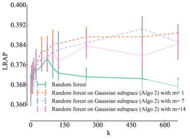
Figure 2: Output randomization with Gaussian projections yield better average precision than the original output space on the “Drug-Interaction” dataset ($n_{\min}=1$ , $t=100$).

We refer the reader to a similar study on the “Delicious” dataset given in the Appendix E (supplementary material), which shows that the interaction between $m$ and $k$ may be different from one dataset to another. It is thus advisable to jointly optimize the value of $m$ and $k$, so as to maximise the tradeoff between accuracy and computing times in a problem and algorithm specific way.

4.5 Alternative output dimension reduction techniques

In this section, we study Algorithm 2 when it is combined with alternative output-space dimensionality reduction techniques. We focus again on the “Delicious” dataset, but similar trends could be observed on other datasets.

Figure 3(a) first compares Gaussian random projections with two other dense projections: Rademacher matrices with $s=1$ (cf. Section 2.2) and compression matrices obtained by sub-sampling (without replacement) Hadamard matrices [8]. We observe that Rademacher and subsample-Hadamard sub-spaces behave very similarly to Gaussian random projections.

In a second step, we compare Gaussian random projections with two (very) sparse projections: first, sparse Rademacher sub-spaces obtained by setting the sparsity parameter $s$ to $3$ and $\sqrt{d}$, selecting respectively about 33% and 2% of the original outputs to compute each component, and second, sub-sampled identity subspaces, similar to [34], where each of the $m$ selected components corresponds to a randomly chosen original label and also preserve sparsity. Sparse projections are very interesting from a computational point of view as they require much less operations to compute the projections but the number of components required for condition (4) to be satisfied is typically higher than for dense projections [24, 8]. Figure 3(b) compares these three projection methods with standard Random Forests on the “delicious” dataset. All three projection methods converge to plain Random Forests as the number of components $m$ increases but their behaviour at low $m$ values are very different. Rademacher projections converge faster with $s=3$ than with $s=1$ and interestingly, the sparsest variant ($s=\sqrt{d}$) has its optimum at $m=1$ and improves in this case over the Random Forests baseline. Random output subspaces converge slower but they lead to a notable improvement of the score over baseline Random Forests. This suggests that although their theoretical guarantees are less good, sparse projections actually provide on this problem a better bias/variance tradeoff than dense ones when used in the context of Algorithm 2.

Another popular dimension reduction technique is the principal component analysis (PCA). In Figure 3(c), we repeat the same experiment to compare PCA with Gaussian random projections. Concerning PCA, the curve is generated in decreasing order of eigenvalues, according to their contribution to the explanation of the output-space variance. We observe that this way of doing is far less effective than the random projection techniques studied previously.

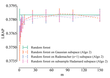
(a) Computing the impurity criterion on a dense Rademacher or on a subsample-Hadamard output sub-space is another efficient way to learn tree ensembles.

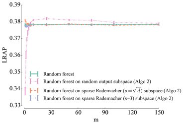
(b) Sparse random projections output sub-space yield better average precision than on the original output space.

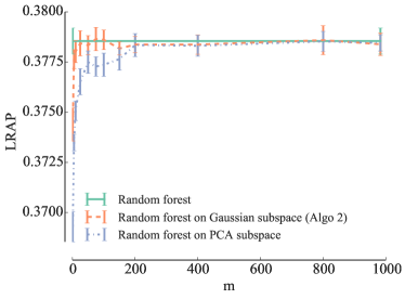
(c) PCA compared with Gaussian subspaces.

Figure 3: “Delicious” dataset, $t=100$, $k=\sqrt{p}$, $n_{\min}=1$.

4.6 Learning stage computing times

Our implementation of the learning algorithms is based on the scikit-learn Python package version 0.14-dev [27]. To fix ideas about computing times, we report these obtained on a Mac Pro 4.1 with a dual Quad-Core Intel Xeon processor at 2.26 GHz, on the “Delicious” dataset. Matrix operation, such as random projections, are performed with the BLAS and the LAPACK from the Mac OS X Accelerate framework. Reported times are obtained by summing the user and sys time of the time UNIX utility.

The reported timings correspond to the following operation: (i) load the dataset in memory, (ii) execute the algorithm. All methods use the same code to build trees. In these conditions, learning a random forest on the original output space ($t=100$, $n_{\min}=1$, $k=\sqrt{d}$) takes 3348  s; learning the same model on a Gaussian output space of size $m=25$ requires 311 s, while $m=1$ and $m=250$ take respectively 236 s and 1088 s. Generating a Gaussian sub-space of size $m=25$ and projecting the output data of the training samples is done in less than 0.25 s, while $m=1$ and $m=250$ takes around 0.07 s and 1 s respectively. The time needed to compute the projections is thus negligible with respect to the time needed for the tree construction.

We see that a speed-up of an order of magnitude could be obtained, while at the same time preserving accuracy with respect to the baseline Random Forests method. Equivalently, for a fixed computing time budget, randomly projecting the output space allows to build more trees and thus to improve predictive performances with respect to standard Random Forests.

5 Conclusions

This paper explores the use of random output space projections combined with tree-based ensemble methods to address large-scale multi-label classification problems. We study two algorithmic variants that either build a tree-based ensemble model on a single shared random subspace or build each tree in the ensemble on a newly drawn random subspace. The second approach is shown theoretically and empirically to always outperform the first in terms of accuracy. Experiments on 24 datasets show that on most problems, using gaussian projections allows to reduce very drastically the size of the output space, and therefore computing times, without affecting accuracy. Remarkably, we also show that by adjusting jointly the level of input and output randomizations and choosing appropriately the projection method, one could also improve predictive performance over the standard Random Forests, while still improving very significantly computing times. As future work, it would be very interesting to propose efficient techniques to automatically adjust these parameters, so as to reach the best tradeoff between accuracy and computing times on a given problem.

To best of our knowledge, our work is the first to study random output projections in the context of multi-output tree-based ensemble methods. The possibility with these methods to relabel tree leaves with predictions in the original output space makes this combination very attractive. Indeed, unlike similar works with linear models [19, 10], our approach only relies on Johnson-Lindenstrauss lemma, and not on any output sparsity assumption, and also does not require to use any output reconstruction method. Besides multi-label classification, we would like to test our method on other, not necessarily sparse, multi-output prediction problems.

Acknowledgements.

Arnaud Joly is research fellow of the FNRS, Belgium. This work is supported by PASCAL2 and the IUAP DYSCO, initiated by the Belgian State, Science Policy Office.

Appendix 0.A Proof of equation (3)

The sum of the variances of $n$ observations drawn from a random vector $y\in\mathbb{R}^{d}$ can be interpreted as a sum of squared euclidean distances between the pairs of observations

$$\operatorname{Var}((y^{i})_{i=1}^{n})=\frac{1}{2n^{2}}\sum_{i=1}^{n}\sum_{j=1}^{n}||y^{i}-y^{j}||^{2}.$$ (a.1)

Proof

$$\operatorname{Var}((y^{i})_{i=1}^{n})$$

$$\stackrel{{\scriptstyle\mbox{\tiny def}}}{{=}}\frac{1}{n}\sum_{i=1}^{n}||y^{i}-\frac{1}{n}\sum_{j=1}^{n}y^{j}||^{2}$$ (a.2)

$$=\frac{1}{n}\sum_{i=1}^{n}(y^{i}-\frac{1}{n}\sum_{j=1}^{n}y^{j})^{T}(y^{i}-\frac{1}{n}\sum_{k=1}^{n}y^{k})$$ (a.3)

$$=\frac{1}{n}\sum_{i=1}^{n}\left({y^{i}}^{T}y^{i}-\frac{2}{n}\sum_{j=1}^{n}{y^{i}}^{T}y^{j}+\frac{1}{n^{2}}\sum_{j=1}^{n}\sum_{k=1}^{n}{y^{j}}^{T}y^{k}\right)$$ (a.4)

$$=\frac{1}{n}\sum_{i=1}^{n}{y^{i}}^{T}y^{i}-\frac{2}{n^{2}}\sum_{i=1}^{n}\sum_{j=1}^{n}{y^{i}}^{T}y^{j}+\frac{1}{n^{2}}\sum_{j=1}^{n}\sum_{k=1}^{n}{y^{j}}^{T}y^{k}$$ (a.5)

$$=\frac{1}{n}\sum_{i=1}^{n}{y^{i}}^{T}y^{i}-\frac{1}{n^{2}}\sum_{i=1}^{n}\sum_{j=1}^{n}{y^{i}}^{T}y^{j}$$ (a.6)

$$=\frac{1}{2n}\sum_{i=1}^{n}{y^{i}}^{T}y^{i}+\frac{1}{2n}\sum_{j=1}^{n}{y^{j}}^{T}y^{j}-\frac{1}{n^{2}}\sum_{i=1}^{n}\sum_{j=1}^{n}{y^{i}}^{T}y^{j}$$ (a.7)

$$=\frac{1}{2n^{2}}\sum_{i=1}^{n}\sum_{j=1}^{n}{y^{i}}^{T}y^{i}+\frac{1}{2n^{2}}\sum_{i=1}^{n}\sum_{j=1}^{n}{y^{j}}^{T}y^{j}-\frac{1}{n^{2}}\sum_{i=1}^{n}\sum_{j=1}^{n}{y^{i}}^{T}y^{j}$$ (a.8)

$$=\frac{1}{2n^{2}}\sum_{i=1}^{n}\sum_{j=1}^{n}\left({y^{i}}^{T}y^{i}+{y^{j}}^{T}y^{j}-2{y^{i}}^{T}y^{j}\right)$$ (a.9)

$$=\frac{1}{2n^{2}}\sum_{i=1}^{n}\sum_{j=1}^{n}||y^{i}-y^{j}||^{2}.$$ (a.10)

Appendix 0.B Proof of Theorem 1

Theorem 1 Given $\epsilon>0$, a sample $(y^{i})_{i=1}^{n}$ of $n$ points $y\in\mathbb{R}^{d}$ and a projection matrix $\Phi\in\mathbb{R}^{m\times d}$ such that for all $i,j\in\{1,\ldots,n\}$ the Johnson-Lindenstrauss lemma holds, we have also:

$$(1-\epsilon)\operatorname{Var}((y^{i})_{i=1}^{n}) \leq\operatorname{Var}((\Phi y^{i}))_{i=1}^{n})$$

$$\leq(1+\epsilon)\operatorname{Var}((y^{i})_{i=1}^{n}).$$ (a.11)

Proof

This result directly follows from the Johnson-Lindenstrauss Lemma and from eqn. (a.1).

From the Johnson-Lindenstrauss Lemma we have for any $i,j$

$$(1-\epsilon)||y^{i}-y^{j}||^{2}\leq||\Phi y^{i}-\Phi y^{j}||^{2}\leq(1+\epsilon)||y^{i}-y^{j}||^{2}.$$ (a.12)

By summing the three terms of (a.12) over all pairs $i,j$ and dividing by $1/(2n^{2})$ and by then using eqn. (a.1), we get eqn. (a.11).

Appendix 0.C Bias/variance analysis

In this subsection, we adapt the bias/variance analysis of randomised supervised learning algorithms carried out in [17], to assess the effect of random output projections in the context of the two algorithms studied in our paper.

0.C.1 Single random trees.

Let us denote by $f(.;ls,\phi,\epsilon):{\cal X}\rightarrow\mathbb{R}^{d}$ a single multi-output (random) tree obtained from a projection matrix $\phi$ (below we use $\Phi$ to denote the corresponding random variable), where $\epsilon$ is the value of a random variable $\varepsilon$ capturing the random perturbation scheme used to build this tree (e.g., bootstrapping and/or random input space selection). Denoting by $Err(f(x;ls,\phi,\epsilon))$ the square error of this model at some point $x\in{\cal X}$ defined by:

$$E_{Y|x}\{||Y-f(x;ls,\phi,\epsilon\})||^{2}\}.$$

The average of this square error can decomposed as follows:

$$E_{LS,\Phi,\varepsilon}\{Err(f(x;LS,\Phi,\varepsilon))\}$$

$$= \sigma^{2}_{R}(x)+||f_{B}(x)-\bar{f}(x)||^{2}+\operatorname{Var}_{LS,\Phi,\varepsilon}\{f(x;LS,\Phi,\varepsilon)\},$$

where

$$\bar{f}(x)\stackrel{{\scriptstyle\text{def}}}{{=}}E_{LS,\Phi,\varepsilon}\{f(x;LS,\Phi,\varepsilon)\},f_{B}(x)=E_{Y|x}\{Y\},$$

and

$$\small\operatorname{Var}_{LS,\Phi,\varepsilon}\{f(x;LS,\Phi,\varepsilon)\}\stackrel{{\scriptstyle\text{def}}}{{=}}E_{LS,\Phi,\varepsilon}\{||f(x;LS,\Phi,\varepsilon)-\bar{f}(x)||^{2}\}$$

The three terms of this decomposition are respectively the residual error, the bias, and the variance of this estimator (at $x$).

The variance term can be further decomposed as follows using the law of total variance:

$$\small\operatorname{Var}_{LS,\Phi,\varepsilon}\{f(x;LS,\Phi,\varepsilon)\}$$ (a.13)

$$= \operatorname{Var}_{LS}\{E_{\Phi,\varepsilon|LS}\{f(x;LS,\Phi,\varepsilon)\}\}$$

$$+E_{LS}\{\operatorname{Var}_{\Phi,\varepsilon|LS}\{f(x;LS,\Phi,\varepsilon)\}\}.$$

The first term is the variance due to the learning sample randomization and the second term is the average variance (over $LS$) due to both the random forest randomization and the random output projection. By using the law of total variance a second time, the second term of (a.13) can be further decomposed as follows:

$$E_{LS}\{\operatorname{Var}_{\Phi,\varepsilon|LS}\{f(x;LS,\Phi,\varepsilon)\}\}$$

$$=E_{LS}\{\operatorname{Var}_{\Phi|LS}\{E_{\varepsilon|LS,\Phi}\{f(x;LS,\Phi,\varepsilon)\}\}\}$$

$$\quad+E_{LS}\{E_{\Phi|LS}\{\operatorname{Var}_{\varepsilon|LS,\Phi}\{f(x;LS,\Phi,\varepsilon)\}\}\}.$$ (a.14)

The first term of this decomposition is the variance due to the random choice of a projection and the second term is the average variance due to the random forest randomization. Note that all these terms are non negative. In what follows, we will denote these three terms respectively $V_{LS}(x)$, $V_{Algo}(x)$, and $V_{proj}(x)$. We thus have:

$$\operatorname{Var}_{LS,\Phi,\varepsilon}\{f(x;LS,\Phi,\varepsilon)\}=V_{LS}(x)+V_{Algo}(x)+V_{Proj}(x),$$

with

$$V_{LS}(x) = \operatorname{Var}_{LS}\{E_{\Phi,\varepsilon|LS}\{f(x;LS,\Phi,\varepsilon)\}\}$$

$$V_{Algo}(x) = E_{LS}\{E_{\Phi|LS}\{\operatorname{Var}_{\varepsilon|LS,\Phi}\{f(x;LS,\Phi,\varepsilon)\}\}\},$$

$$V_{Proj}(x) = E_{LS}\{\operatorname{Var}_{\Phi|LS}\{E_{\varepsilon|LS,\Phi}\{f(x;LS,\Phi,\varepsilon)\}\}\},$$

0.C.2 Ensembles of $t$ random trees.

When the random projection is fixed for all $t$ trees in the ensemble (Algorithm 1), the algorithm computes an approximation, denoted $f_{1}(x;ls,\phi,\epsilon^{t})$, that takes the following form:

$$f_{1}(x;ls,\phi,\epsilon^{t})=\frac{1}{t}\sum_{i=1}^{t}f(x;ls,\phi,\epsilon_{i}),$$

where $\epsilon^{t}=(\epsilon_{1},\ldots,\epsilon_{t})$ a vector of i.i.d. values of the random variable $\varepsilon$. When a different random projection is chosen for each tree (Algorithm 2), the algorithm computes an approximation, denoted by $f_{2}(x;ls,\phi^{t},\epsilon^{t})$, of the following form:

$$f_{2}(x;ls,\phi^{t},\epsilon^{t})=\frac{1}{t}\sum_{i=1}^{t}f(x;ls,\phi_{i},\epsilon_{i}),$$

where $\phi^{t}=(\phi_{1},\ldots,\phi_{t})$ is also a vector of i.i.d. random projection matrices.

We would like to compare the average errors of these two algorithms with the average errors of the original single tree method, where the average is taken for all algorithms over their random parameters (that include the learning sample).

Given that all trees are grown independently of each other, one can show that the average models corresponding to each algorithm are equal:

$$\bar{f}(x) = E_{LS,\Phi,\varepsilon^{t}}\{f_{1}(x;LS,\Phi,\varepsilon^{t})\}$$

$$= E_{LS,\Phi^{t},\varepsilon^{t}}\{f_{2}(x;LS,\Phi^{t},\varepsilon^{t})\}.$$

They thus all have the exact same bias (and residual error) and differ only in their variance.

Using the same argument, the first term of the variance decomposition in (a.13), ie. $V_{LS}(x)$, is the same for all three algorithms since:

$$E_{\Phi,\varepsilon|LS}\{f(x;LS,\Phi,\varepsilon)\}$$

$$= E_{\Phi,\varepsilon^{t}|LS}\{f_{1}(x;LS,\Phi,\varepsilon^{t})\}$$

$$= E_{\Phi^{t},\varepsilon^{t}|LS}\{f_{2}(x;LS,\Phi^{t},\varepsilon^{t})\}.$$

Their variance thus only differ in the second term in (a.13).

Again, because of the conditional independence of the ensemble terms given the $ls$ and projection matrix $\phi$, Algorithm 1, which keeps the output projection fixed for all trees, is such that

$$E_{\epsilon^{t}|LS,\Phi}\{f_{1}(x;LS,\Phi,\varepsilon^{t})\}=E_{\epsilon|LS,\Phi}\{f(x;LS,\Phi,\varepsilon)\}$$

and

$$\operatorname{Var}_{\varepsilon^{t}|LS,\Phi}\{f_{1}(x;LS,\Phi,\varepsilon^{t})\}=\frac{1}{t}\operatorname{Var}_{\varepsilon|LS,\Phi}\{f(x;LS,\Phi,\varepsilon)\}.$$

It thus divides the second term of (a.14) by the number $t$ of ensemble terms. Algorithm 2, on the other hand, is such that:

$$\operatorname{Var}_{\Phi^{t},\varepsilon^{t}|LS}\{f_{2}(x;LS,\Phi,\varepsilon^{t})\}=\frac{1}{t}\operatorname{Var}_{\Phi,\varepsilon|LS}\{f(x;LS,\Phi,\varepsilon)\},$$

and thus divides the second term of (a.13) by $t$.

Putting all these results together one gets that:

$$E_{LS,\Phi,\varepsilon}\{Err(f(x;LS,\Phi,\varepsilon^{t}))\}$$

$$=\sigma^{2}_{R}(x)+B^{2}(x)+V_{LS}(x)+V_{Algo}(x)+V_{Proj}(x),$$

$$E_{LS,\Phi,\varepsilon^{t}}\{Err(f_{1}(x;LS,\Phi,\varepsilon^{t}))\}$$

$$=\sigma^{2}_{R}(x)+B^{2}(x)+V_{LS}(x)+\frac{V_{Algo}(x)}{t}+V_{Proj}(x),$$

$$E_{LS,\Phi^{t},\varepsilon^{t}}\{Err(f_{2}(x;LS,\Phi^{t},\varepsilon^{t}))\}$$

$$=\sigma^{2}_{R}(x)+B^{2}(x)+V_{LS}(x)+\frac{V_{Algo}(x)+V_{Proj}(x)}{t}.$$

Given that all terms are positive, this result clearly shows that Algorithm 2 can not be worse than Algorithm 1.

Appendix 0.D Description of the datasets

Experiments are performed on several multi-label datasets: the yeast [16] dataset in the biology domain; the corel5k [15] and the scene [5] datasets in the image domain; the emotions [35] and the CAL500 [36] datasets in the music domain; the bibtex [21], the bookmarks [21], the delicious [32], the enron [22], the EUR-Lex (subject matters, directory codes and eurovoc descriptors) [26] the genbase [14], the medical, the tmc2007 [31] datasets in the text domain and the mediamill [30] dataset in the video domain.

Several hierarchical classification tasks are also studied to increase the diversity in the number of label and treated as multi-label classification task. Each node of the hierarchy is treated as one label. Nodes of the hierarchy which never occured in the training or testing set were removed. The reuters [29], WIPO [29] datasets are from the text domain. The Diatoms [13] dataset is from the image domain. SCOP-GO [11], Yeast-GO [3] and Expression-GO [37] are from the biological domain. Missing values in the Expression-GO dataset were inferred using the median for continuous features and the most frequent value for categorical features using the entire dataset. The inference of a drug-protein interaction network [38] is also considered either using the drugs to infer the interactions with the protein (drug-interaction), either using the proteins to infer the interactions with the drugs (protein-interaction).

Those datasets were selected to have a wide range of number of outputs $d$. Their basic characteristics are summarized at Table 2. For more information on a particular dataset, please see the relevant paper.

Table 2: Selected datasets have a number of labels $d$ ranging from 6 up to 3993 in the biology, the text, the image, the video or the music domain. Each dataset has $n_{LS}$ training samples, $n_{TS}$ testing samples and $p$ input features.

Datasets	$n_{LS}$	$n_{TS}$	$p$	$d$
emotions	391	202	72	6
scene	1211	1196	2407	6
yeast	1500	917	103	14
tmc2007	21519	7077	49060	22
genbase	463	199	1186	27
reuters	2500	5000	19769	34
medical	333	645	1449	45
enron	1123	579	1001	53
mediamill	30993	12914	120	101
Yeast-GO	2310	1155	5930	132
bibtex	4880	2515	1836	159
CAL500	376	126	68	174
WIPO	1352	358	74435	188
EUR-Lex (subject matters)	19348	10-cv	5000	201
bookmarks	65892	21964	2150	208
diatoms	2065	1054	371	359
corel5k	4500	500	499	374
EUR-Lex (directory codes)	19348	10-cv	5000	412
SCOP-GO	6507	3336	2003	465
delicious	12920	3185	500	983
drug-interaction	1396	466	660	1554
protein-interaction	1165	389	876	1862
Expression-GO	2485	551	1288	2717
EUR-Lex (eurovoc descriptors)	19348	10-cv	5000	3993

Appendix 0.E Experiments with Extra trees

In this section, we carry out experiments combining Gaussian random projections (with $m\in\{1,\ln{d},d\}$) with the Extra Trees method of [17] (see Section 2.1 of the paper for a very brief description of this method). Results on 23 datasets are compiled in Table 3.

Like for Random Forests, we observe that for all 23 datasets taking $m=d$ leads to a similar average precision to the standard Random Forests, ie. no difference superior to one standard deviation of the error. This is already the case with $m=1$ for 12 datasets and with $m=\ln{d}$ for 4 more datasets. Interestingly, on 3 datasets with $m=1$ and 3 datasets with $m=\ln{d}$, the increased randomization brought by the projections actually improves average precision with respect to standard Random Forests (bold values in Table 3).

Table 3: Experiments with Gaussian projections and Extra Trees (($t=100$, $n_{\min}=1$, $k=\sqrt{p}$). See Section 4.3 and Table 1 in the paper for the protocol. Mean scores in the last three columns are underlined if they show a negative difference with respect to the standard Random Forests of more than one standard deviation. Bold values highlight improvement over standard RF of more than one standard deviation.

Datasets	Extra trees		Extra trees on Gaussian sub-space
			$m=1$		$m=\lfloor 0.5+\ln{d}\rfloor$		$m=d$
emotions	$0.81$	$\pm 0.01$	$0.81$	$\pm 0.014$	$0.80$	$\pm 0.013$	$0.81$	$\pm 0.014$
scene	$0.873$	$\pm 0.004$	$0.876$	$\pm 0.003$	$0.877$	$\pm 0.007$	$0.878$	$\pm 0.006$
yeast	$0.757$	$\pm 0.008$	$0.746$	$\pm 0.004$	$0.752$	$\pm 0.009$	$0.757$	$\pm 0.01$
tmc2017	$0.782$	$\pm 0.003$	$0.759$	$\pm 0.004$	$0.77$	$\pm 0.002$	$0.779$	$\pm 0.002$
genbase	$0.987$	$\pm 0.005$	$0.991$	$\pm 0.004$	$0.992$	$\pm 0.001$	$0.992$	$\pm 0.005$
reuters	$0.88$	$\pm 0.003$	$0.88$	$\pm 0.003$	$0.878$	$\pm 0.004$	$0.88$	$\pm 0.004$
medical	$0.855$	$\pm 0.008$	$\bf 0.867$	$\pm 0.009$	$\bf 0.872$	$\pm 0.006$	$0.862$	$\pm 0.008$
enron	$0.66$	$\pm 0.01$	$0.65$	$\pm 0.01$	$0.663$	$\pm 0.008$	$0.66$	$\pm 0.01$
mediamill	$0.786$	$\pm 0.002$	$0.778$	$\pm 0.002$	$0.781$	$\pm 0.002$	$0.784$	$\pm 0.001$
Yeast-GO	$0.49$	$\pm 0.009$	$0.47$	$\pm 0.01$	$0.482$	$\pm 0.008$	$0.48$	$\pm 0.01$
bibtex	$0.584$	$\pm 0.005$	$0.538$	$\pm 0.005$	$0.564$	$\pm 0.004$	$0.583$	$\pm 0.004$
CAL500	$0.5$	$\pm 0.007$	$0.502$	$\pm 0.008$	$0.499$	$\pm 0.007$	$0.503$	$\pm 0.009$
WIPO	$0.52$	$\pm 0.01$	$0.474$	$\pm 0.007$	$0.49$	$\pm 0.01$	$0.515$	$\pm 0.006$
EUR-Lex (subj.)	$0.845$	$\pm 0.006$	$0.834$	$\pm 0.004$	$0.838$	$\pm 0.003$	$0.845$	$\pm 0.005$
bookmarks	$0.453$	$\pm 0.002$	$0.436$	$\pm 0.002$	$0.444$	$\pm 0.003$	$0.452$	$\pm 0.002$
diatoms	$0.73$	$\pm 0.01$	$0.69$	$\pm 0.01$	$0.71$	$\pm 0.01$	$0.73$	$\pm 0.01$
corel5k	$0.285$	$\pm 0.009$	$\bf 0.313$	$\pm 0.011$	$\bf 0.309$	$\pm 0.009$	$0.285$	$\pm 0.011$
EUR-Lex (dir.)	$0.815$	$\pm 0.007$	$0.805$	$\pm 0.006$	$0.807$	$\pm 0.009$	$0.815$	$\pm 0.007$
SCOP-GO	$0.778$	$\pm 0.005$	$0.782$	$\pm 0.004$	$0.782$	$\pm 0.006$	$0.778$	$\pm 0.005$
delicious	$0.354$	$\pm 0.003$	$\bf 0.36$	$\pm 0.004$	$\bf 0.358$	$\pm 0.004$	$0.355$	$\pm 0.003$
drug-interaction	$0.353$	$\pm 0.011$	$\bf 0.375$	$\pm 0.017$	$0.364$	$\pm 0.014$	$0.355$	$\pm 0.016$
protein-interaction	$0.299$	$\pm 0.013$	$0.307$	$\pm 0.009$	$0.305$	$\pm 0.012$	$0.306$	$\pm 0.017$
Expression-GO	$0.231$	$\pm 0.007$	$0.218$	$\pm 0.005$	$0.228$	$\pm 0.005$	$0.235$	$\pm 0.005$

Appendix 0.F Input vs output space randomization on “Delicious”

In this section, we carry out the same experiment as in Section 4.4 of the main paper but on the “Delicious” dataset. Figure 4 shows the evolution of the accuracy for growing values of $k$ (i.e. decreasing strength of the input space randomization), for three different values of $m$ (in this case $m\in\left\{1,\ln{d},2\ln{d}\right\}$) on a Gaussian output space.

Like on “Drug-interaction” (see Figure 2 of the paper), using low-dimensional output spaces makes the method more robust with respect to over-fitting as $k$ increases. However, unlike on “Drug-interaction”, it is not really possible to improve over baseline Random Forests by tuning jointly input and output randomization. This shows that the interaction between $m$ and $k$ may be different from one dataset to another.

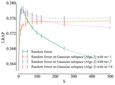
Figure 4: “Delicious” dataset: $n_{\min}=1$; $t=100$.

References

- [1] Achlioptas, D.: Database-friendly random projections: Johnson-lindenstrauss with binary coins. J. Comput. Syst. Sci. 66(4), 671–687 (2003)
- [2] Agrawal, R., Gupta, A., Prabhu, Y., Varma, M.: Multi-label learning with millions of labels: recommending advertiser bid phrases for web pages. In: Proceedings of the 22nd international conference on World Wide Web. pp. 13–24. International World Wide Web Conferences Steering Committee (2013)
- [3] Barutcuoglu, Z., Schapire, R.E., Troyanskaya, O.G.: Hierarchical multi-label prediction of gene function. Bioinformatics 22(7), 830–836 (2006)
- [4] Blockeel, H., De Raedt, L., Ramon, J.: Top-down induction of clustering trees. In: Proceedings of ICML 1998. pp. 55–63 (1998)
- [5] Boutell, M.R., Luo, J., Shen, X., Brown, C.M.: Learning multi-label scene classification. Pattern recognition 37(9), 1757–1771 (2004)
- [6] Breiman, L.: Random forests. Machine Learning 45(1), 5–32 (2001)
- [7] Breiman, L., Friedman, J.H., Olshen, R.A., Stone, C.J.: Classification and Regression Trees. Wadsworth (1984)
- [8] Candes, E.J., Plan, Y.: A probabilistic and ripless theory of compressed sensing. Information Theory, IEEE Transactions on 57(11), 7235–7254 (2011)
- [9] Cheng, W., Hüllermeier, E., Dembczynski, K.J.: Bayes optimal multilabel classification via probabilistic classifier chains. In: Proceedings of the 27th international conference on machine learning (ICML-10). pp. 279–286 (2010)
- [10] Cisse, M.M., Usunier, N., Artières, T., Gallinari, P.: Robust bloom filters for large multilabel classification tasks. In: Burges, C., Bottou, L., Welling, M., Ghahramani, Z., Weinberger, K. (eds.) Advances in Neural Information Processing Systems 26, pp. 1851–1859 (2013)
- [11] Clare, A.: Machine learning and data mining for yeast functional genomics. Ph.D. thesis, University of Wales Aberystwyth, Aberystwyth, Wales, UK (2003)
- [12] Dekel, O., Shamir, O.: Multiclass-multilabel classification with more classes than examples. In: International Conference on Artificial Intelligence and Statistics. pp. 137–144 (2010)
- [13] Dimitrovski, I., Kocev, D., Loskovska, S., Džeroski, S.: Hierarchical classification of diatom images using ensembles of predictive clustering trees. Ecological Informatics 7(1), 19–29 (2012)
- [14] Diplaris, S., Tsoumakas, G., Mitkas, P.A., Vlahavas, I.: Protein classification with multiple algorithms. In: Advances in Informatics, pp. 448–456. Springer (2005)
- [15] Duygulu, P., Barnard, K., de Freitas, J.F.G., Forsyth, D.A.: Object recognition as machine translation: Learning a lexicon for a fixed image vocabulary. In: Computer Vision—ECCV 2002, pp. 97–112. Springer (2006)
- [16] Elisseeff, A., Weston, J.: A kernel method for multi-labelled classification. In: Advances in neural information processing systems. pp. 681–687 (2001)
- [17] Geurts, P., Ernst, D., Wehenkel, L.: Extremely randomized trees. Machine Learning 63(1), 3–42 (2006)
- [18] Geurts, P., Wehenkel, L., d’Alché Buc, F.: Kernelizing the output of tree-based methods. In: Proceedings of the 23rd international conference on Machine learning. pp. 345–352. Acm (2006)
- [19] Hsu, D., Kakade, S., Langford, J., Zhang, T.: Multi-label prediction via compressed sensing. In: Bengio, Y., Schuurmans, D., Lafferty, J., Williams, C.K.I., Culotta, A. (eds.) Advances in Neural Information Processing Systems 22, pp. 772–780 (2009)
- [20] Johnson, W.B., Lindenstrauss, J.: Extensions of Lipschitz mappings into a Hilbert space. Contemporary mathematics 26(189-206), 1 (1984)
- [21] Katakis, I., Tsoumakas, G., Vlahavas, I.: Multilabel text classification for automated tag suggestion. In: Proceedings of the ECML/PKDD (2008)
- [22] Klimt, B., Yang, Y.: The enron corpus: A new dataset for email classification research. In: Machine learning: ECML 2004, pp. 217–226. Springer (2004)
- [23] Kocev, D., Vens, C., Struyf, J., Dzeroski, S.: Tree ensembles for predicting structured outputs. Pattern Recognition 46(3), 817–833 (2013)
- [24] Li, P., Hastie, T.J., Church, K.W.: Very sparse random projections. In: Proceedings of the 12th ACM SIGKDD international conference on Knowledge discovery and data mining. pp. 287–296. ACM (2006)
- [25] Madjarov, G., Kocev, D., Gjorgjevikj, D., Dzeroski, S.: An extensive experimental comparison of methods for multi-label learning. Pattern Recognition 45(9), 3084–3104 (2012)
- [26] Mencía, E.L., Fürnkranz, J.: Efficient multilabel classification algorithms for large-scale problems in the legal domain. In: Semantic Processing of Legal Texts, pp. 192–215. Springer (2010)
- [27] Pedregosa, F., Varoquaux, G., Gramfort, A., Michel, V., Thirion, B., Grisel, O., Blondel, M., Prettenhofer, P., Weiss, R., Dubourg, V., et al.: Scikit-learn: Machine learning in python. The Journal of Machine Learning Research 12, 2825–2830 (2011)
- [28] Read, J., Pfahringer, B., Holmes, G., Frank, E.: Classifier chains for multi-label classification. In: Buntine, W., Grobelnik, M., Mladenić, D., Shawe-Taylor, J. (eds.) Machine Learning and Knowledge Discovery in Databases, Lecture Notes in Computer Science, vol. 5782, pp. 254–269. Springer Berlin Heidelberg (2009)
- [29] Rousu, J., Saunders, C., Szedmak, S., Shawe-Taylor, J.: Learning hierarchical multi-category text classification models. In: Proceedings of the 22nd international conference on Machine learning. pp. 744–751. ACM (2005)
- [30] Snoek, C.G.M., Worring, M., Van Gemert, J.C., Geusebroek, J.M., Smeulders, A.W.M.: The challenge problem for automated detection of 101 semantic concepts in multimedia. In: Proceedings of the 14th annual ACM international conference on Multimedia. pp. 421–430. ACM (2006)
- [31] Srivastava, A.N., Zane-Ulman, B.: Discovering recurring anomalies in text reports regarding complex space systems. In: Aerospace Conference, 2005 IEEE. pp. 3853–3862. IEEE (2005)
- [32] Tsoumakas, G., Katakis, I., Vlahavas, I.: Effective and efficient multilabel classification in domains with large number of labels. In: Proc. ECML/PKDD 2008 Workshop on Mining Multidimensional Data (MMD’08). pp. 30–44 (2008)
- [33] Tsoumakas, G., Katakis, I., Vlahavas, I.P.: Random k-labelsets for multilabel classification. IEEE Trans. Knowl. Data Eng. 23(7), 1079–1089 (2011)
- [34] Tsoumakas, G., Vlahavas, I.: Random k-labelsets: An ensemble method for multilabel classification. In: Machine Learning: ECML 2007, pp. 406–417. Springer (2007)
- [35] Tsoumakas, K.T.G., Kalliris, G., Vlahavas, I.: Multi-label classification of music into emotions. In: ISMIR 2008: Proceedings of the 9th International Conference of Music Information Retrieval. p. 325. Lulu. com (2008)
- [36] Turnbull, D., Barrington, L., Torres, D., Lanckriet, G.: Semantic annotation and retrieval of music and sound effects. Audio, Speech, and Language Processing, IEEE Transactions on 16(2), 467–476 (2008)
- [37] Vens, C., Struyf, J., Schietgat, L., Džeroski, S., Blockeel, H.: Decision trees for hierarchical multi-label classification. Machine Learning 73(2), 185–214 (2008)
- [38] Yamanishi, Y., Pauwels, E., Saigo, H., Stoven, V.: Extracting sets of chemical substructures and protein domains governing drug-target interactions. Journal of chemical information and modeling 51(5), 1183–1194 (2011)
- [39] Zhou, T., Tao, D.: Multi-label subspace ensemble. In: International Conference on Artificial Intelligence and Statistics. pp. 1444–1452 (2012)