Connecting speeds, directions and arrival times of 22 coronal mass ejections from the Sun to 1 AU

Abstract

Forecasting the in situ properties of coronal mass ejections (CMEs) from remote images is expected to strongly enhance predictions of space weather, and is of general interest for studying the interaction of CMEs with planetary environments. We study the feasibility of using a single heliospheric imager (HI) instrument, imaging the solar wind density from the Sun to 1 AU, for connecting remote images to in situ observations of CMEs. We compare the predictions of speed and arrival time for 22 CMEs (in 2008-2012) to the corresponding interplanetary coronal mass ejection (ICME) parameters at in situ observatories (STEREO PLASTIC/IMPACT, Wind SWE/MFI). The list consists of front- and backsided, slow and fast CMEs (up to 2700 km s^-1). We track the CMEs to $34.9\pm 7.1$ degrees elongation from the Sun with J-maps constructed using the SATPLOT tool, resulting in prediction lead times of $-26.4\pm 15.3$ hours. The geometrical models we use assume different CME front shapes (Fixed-$\Phi$, Harmonic Mean, Self-Similar Expansion), and constant CME speed and direction. We find no significant superiority in the predictive capability of any of the three methods. The absolute difference between predicted and observed ICME arrival times is $8.1\pm 6.3$ hours ($rms$ value of 10.9h). Speeds are consistent to within $284\pm 288$ km s^-1. Empirical corrections to the predictions enhance their performance for the arrival times to $6.1\pm 5.0$ hours ($rms$ value of 7.9h), and for the speeds to $53\pm 50$ km s^-1. These results are important for Solar Orbiter and a space weather mission positioned away from the Sun–Earth line.

.

1. Introduction

Storms from the Sun, known as coronal mass ejections (CMEs), are massive, quickly expanding expulsions of plasma threaded by magnetic fields, originating from both quiescent and active regions in the Sun’s corona. Over a distance of a few solar radii, they may accelerate up to speeds of 3000 kilometers per second in rare cases, and subsequently propagate through the solar wind away from the Sun. CMEs are able to reach 1 AU in half a day in the most extreme cases, and are the source of the strongest disturbances in the Earth’s magnetosphere (e.g. Zhang et al., 2007).

Forecasting their general properties, such as propagation direction and speed close to the Sun and in the interplanetary medium, as well as their arrival time and arrival speed at a given planet or spacecraft, is a major issue in the field of heliophysics. Moreover, the science that underlies our ability to predict CME arrival times and speeds with high precision, which is at the heart of a reliable, real-time space weather forecast, is still not well understood, with average errors of the order of 0.5 to 1 day and several $100$ km s^-1, respectively (e.g. Gopalswamy et al., 2001). Recent advances in analysing multi-point imaging data has improved these classic values for a few CME events by roughly a factor of two (Mishra & Srivastava, 2013; Colaninno et al., 2013). While this is clearly of greatest interest for the location of the Earth, predictions and parameters of CMEs impacting Mercury, Venus, Mars, Jupiter and Saturn are also essential for studying their interaction with other planetary environments (e.g. Baker et al., 2013).

The Solar TErrestrial RElations Observatory (STEREO, Kaiser et al., 2008), launched in late 2006, consists of two spacecraft, one ahead (STEREO-A) and one behind the Earth (STEREO-B) in orbits around the Sun. Each year, each spacecraft separates from the Earth by about 22^∘ in heliocentric longitude. Its SECCHI instruments seamlessly image CMEs from the Sun to 1 AU and beyond. We are able to extract CME speeds and directions from the images in order to pin down CME evolution and assess CME predictions (e.g. Möstl et al., 2009b; Wood et al., 2010; Liu et al., 2010a; Lugaz et al., 2010; Lynch et al., 2010; Savani et al., 2010; Davis et al., 2011; Liewer et al., 2011; Möstl et al., 2011; Savani et al., 2012; Rollett et al., 2012; Liu et al., 2013; Mishra & Srivastava, 2013; Colaninno et al., 2013; Davies et al., 2013). Even numerical simulations have been employed to enhance our ability to derive the physics of solar wind structures from heliospheric imaging (e.g. Lugaz et al., 2009, 2011; Xiong et al., 2013a, b; Rollett et al., 2013). A concerted campaign to analyse the series of CMEs launched by the Sun on 2010 August 1 has also revealed many details of CME propagation and their 3D evolution for interacting CMEs (Liu et al., 2012; Harrison et al., 2012; Möstl et al., 2012; Webb et al., 2013; Temmer et al., 2012).

A deceptively simple but persistent problem in the analysis of CMEs has been to find definite connections between the remote images of CMEs (Illing & Hundhausen, 1985), taken by coronagraph or heliospheric imager instruments, and the signatures of CMEs in time series of plasma and magnetic field measurements taken directly (in situ) in the solar wind (Burlaga et al., 1981). Current space-based coronagraphs on 3 different spacecraft (STEREO-A/COR1/COR2, STEREO-B/COR1/COR2, and SOHO/LASCO) can image a CME in its entirety during its “birth” and early propagation phase ($1-15$ solar radii). These instruments provide white-light images of CMEs projected into the plane of the sky, i.e. the plane perpendicular to the Sun–spacecraft line. As the CME propagates further away from the Sun, heliospheric imager (HI) instruments image, in white–light, its integrated density signature around the so-called “Thomson surface” (Vourlidas & Howard, 2006) or “Thomson plateau” (Howard & DeForest, 2012b) at elongation angles of 4-88^∘ from the Sun (for STEREO/HI). Because of the wider viewing angle, the interpretation and analysis of HI data is more complex compared to coronagraphs and not yet fully understood (e.g. Rouillard, 2011; Howard & DeForest, 2012b).

When a CME hits a spacecraft with in situ instruments onboard that are capable of characterizing the solar wind plasma and magnetic fields, it leads to distinct signatures in the time series of the measured parameters. Often, a shock is followed by a sheath region in front of a magnetic driver, which is either an irregular structure or a large-scale magnetic flux rope (e.g. Burlaga et al., 1981; Bothmer & Schwenn, 1998; Lynch et al., 2003; Leitner et al., 2007; Möstl et al., 2009a; Richardson & Cane, 2010; Isavnin et al., 2013; Al-Haddad et al., 2013). We call the interval including all of these signatures an “interplanetary CME” or “ICME”. Troughout this paper, we use the term “CMEs” for events observed in images and “ICMEs” for ejecta identified from in situ measurements. However, these measurements of the in situ solar wind give a detailed but otherwise extremely limited and localized view of a CME at the position of the spacecraft near 1 AU. At this distance, a CME has already expanded into an enormous structure, covering up to around 100^∘ in heliocentric longitude and several tenths of an AU along the radial direction to the Sun (Burlaga et al., 1981; Bothmer & Schwenn, 1998; Liu et al., 2005; Richardson & Cane, 2010; Wood et al., 2010; Möstl et al., 2012). Thus, progressing further from the Sun leads to less and less information on the global structure of the CME, which is increasingly hard to interpret, providing a first explanation for the difficulties in linking the datasets.

As a background to our study, it needs to be understood that CMEs are almost never really single entities, but they react to their coronal and heliospheric environments (e.g. Temmer et al., 2011; Kilpua et al., 2012; Rollett et al., 2012). A possible general paradigm of CME propagation through the solar wind has recently emerged. Liu et al. (2013) state a picture of Sun–to–Earth propagation of fast CMEs, derived from a joint analysis using stereoscopic heliospheric images, radio and in situ observations of three CME events: fast CMEs impulsively accelerate close to the Sun, followed by a rapid deceleration out to about 0.4  AU, culminating in an almost constant speed propagation phase (see also, e.g., Gopalswamy et al., 2001, for earlier, similar ideas).

Our paper addresses the problem of seamlessly connecting CMEs from the Sun to 1 AU in two ways. First, we establish a list of suitable CME events from 2008-2012, using observations by coronagraphs, heliospheric imagers and in situ instruments onboard the STEREO and Wind spacecraft, and model the imaging observations using single-spacecraft state-of-the-art-“geometrical modeling” methods. Secondly, we use these connections to enhance our understanding of CME propagation and their prediction, focusing on the improvement of methods to extract CME parameters from heliospheric imager data. Our study builds on the results of Lugaz et al. (2012), who analyzed CMEs in STEREO/HI data that impacted the other STEREO spacecraft during the interval 2008–2010. This study established that predictions of speeds and arrival times for slow CMEs are roughly consistent with corresponding in situ parameters, and demonstrated the possibility for succesfully predicting CMEs that propagate behind the limb or on the backside of the Sun as viewed from HI. However, our paper goes further along several, critical avenues: we included modeling with the new Self-Similar Expansion Fitting (SSEF) technique (Davies et al., 2012), which allows more flexibility for the CME width in the solar equatorial plane than previous models, which were either point-like (Fixed-$\Phi$, Sheeley et al., 1999; Rouillard et al., 2008) or extremely wide (Harmonic Mean, Lugaz et al., 2009, 2010). In addition, we now have STEREO data of very fast CMEs ($>2000$ km s^-1) available, and we mainly discuss Earth-directed events. The STEREO separation from Earth increased from 22^∘ in early 2008 to 120^∘ in mid 2012, thus we include in our study backsided events (from the point of view of a STEREO spacecraft), similar to Lugaz et al. (2012).

Several lines of research have recently converged to make this work possible, apart from having available the remote STEREO observatories in conjunction with the Wind spacecraft (the latter at the Sun-Earth Lagrangian 1 or L1 point): (1) the existence of software packages (i.e., SATPLOT and croissant modeling) to easily extract and fit CMEs in STEREO/COR2 and HI data, (2) the development of mature models to obtain CME speeds and directions from heliospheric imagers, and (3) the rise of solar cycle 24 which culminated in several very fast coronal mass ejections. All this now gives us the opportunity to study the potentially most geoeffective events with multi–point in situ and imaging data (e.g. Liu et al., 2013; Davies et al., 2013).

The connections established in our paper may be used by other researchers to benchmark any empirical or numerical propagation model of CMEs. We need to emphasize that our paper focuses on establishing connections between the datasets, which means that we track CMEs as far as possible through the HI data, up to 30–40^∘ elongation from the Sun. For this reason the prediction lead times, which are the differences between the last data points used for extracting CME parameters, and the actual in situ arrival times, are relatively short, of the order of one day. This should be kept in mind when discussing our results for the errors in CME speeds and arrival times. Shorter tracks in HI must be used in order to increase the prediction lead time to values suitable for real time forecasting, namely from more than one day for fast CMEs to several days for slow CMEs. Such an analysis was carried out by Möstl et al. (2011) for a case study, and is the aim of future studies that will exploit our full dataset, consisting of 22 CME events. The differences in speeds and arrival times that we derive from comparing the HI data to the in situ data thus show how well a HI system configured as on STEREO can perform for CME forecasting.

2. Methods

This section illustrates the observations and models we used to extract CME parameters from various imaging and in situ data. We chose the events in our list by the criteria that each CME has (1) clear in situ signatures and (2) a clear track in J-maps from one STEREO/HI instrument. We then tracked back the CME in the HI J-map to the coronagraph images to find the corresponding CME observations in the corona. We do not attempt to provide a full list of all CMEs directed towards Earth and STEREO during the time between April 2008 and July 2012. However, some of the brightest, fastest and best-studied events in this time-range show up in our list. A well observed, Earth-directed CME that left the Sun on 2012 July 12 and arrived at Earth on 2012 July 14 serves to demonstrate our data pipeline.

2.1. Croissant modeling

The so-called “croissant” model, also known as “Graduated Cylindrical Shell” (GCS) model, is a very well tested tool, available in the IDL SolarSoft package, for deriving the initial directions and speeds of CMEs in the fields of view of the STEREO/COR2 coronagraph, covering 2.5–15.6 $R_{\odot}$ (Thernisien et al., 2006, 2009). At least two viewpoints are needed. Sometimes, the additional viewpoint of the SOHO/LASCO C2 and C3 coronagraphs at the near-Earth L1 point is used, to either give the second view or to provide a third. C2 and C3, combined, cover a distance of 1.5–30 $R_{\odot}$ (Brueckner et al., 1995). The model has also been recently extended for the fields of view of heliospheric imaging (Colaninno et al., 2013), but we will use it in the classic way for analyzing coronagraph images only. Essentially, the model approximates the CME shape as a bent tube which is reminiscent of a croissant, with the mass distributed uniformly on its surface. This shape was chosen to be consistent with a geometry of the CME internal magnetic field as a bent, cylindrical magnetic flux rope. The application of the model consists of manually adjusting parameters that define the CME shape and direction to best fit images of the CME provided by coronagraphs. The major advantage of using this model is that it provides reliable results for the initial 3D propagation direction and initial speed of a CME, free of projection effects. The downside is that not every CME can be approximated by the shape of a croissant, and often CMEs occur within a few hours of each other, making it difficult to distinguish the different physical parts of each CME. Nevertheless, Vourlidas et al. (2013) found that, close to the Sun, at least $40$% of CMEs possessed a flux-rope like structure. We refer the reader to an extensive discussion on the morphology of CMEs in coronagraphs that is provided by those authors.

As an example, the top row in Figure 1 shows images of the 2012 July 12 17:24 UT CME, and the bottom row a green grid of the croissant model overlaid on the same images. It can be seen that the croissant represents the shape of the CME well in all 3 viewpoints. It becomes clear that this CME is roughly directed towards the Earth, appearing as a full halo in SOHO/LASCO, and being directed to solar west from STEREO-B, and to solar east from STEREO-A. To get the CME initial speed $V_{\mathrm{init}}$, we linearly fit height-time measurements for the croissant’s apex over a few data points (e.g. Colaninno et al., 2013). Thus, $V_{\mathrm{init}}$ is an average speed between 2.5–15.6 $R_{\odot}$. The initial CME direction is similarly obtained by adjusting the wire-grid model to the images, and averages over a few data points define the initial CME direction in heliocentric longitude ($\Phi_{\mathrm{init;Earth}}$) in the solar equatorial plane, with the Earth as a reference point at 0^∘ longitude.

Common errors associated with croissant modeling are $\pm$10^∘ in heliocentric longitude for the CME propagation direction, and $\pm$10% of the average CME speed (e.g. Thernisien et al., 2009; Temmer et al., 2012). In Table 1, all results derived with the croissant model are summarized in columns 2–4, including the time $t_{\mathrm{COR2}}$ of the first observation in STEREO-A/COR2 images, the initial direction with respect to Earth ($\Phi_{\mathrm{init;Earth}}$) and the initial speed ($V_{\mathrm{init}}$). For events 16 to 24 in Table 1, we have used 3 viewpoints (STEREO-A/B and SOHO), and for the other events the 2 viewpoints as provided by STEREO-A/B. For Earth-directed CMEs, which appear symmetric in STEREO-A/B, an additional viewpoint provides more reliable results (Vourlidas et al., 2011).

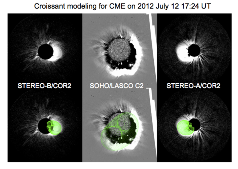
Figure 1.— Croissant modeling of the 2012 July 12 CME on 17:24 UT. From left to right: STEREO-B/COR2, SOHO-LASCO C2, and STEREO-A/COR2. The top row shows the white-light image, the bottom row a green grid of the tube-like croissant model overlaid. The separation of STEREO-B to Earth was 115^∘ in heliocentric longitude, and STEREO-A was 120^∘ ahead of Earth.

2.2. Geometrical modeling

Figure 2 is a summary of the application and the results of the geometrical modeling techniques. Figure 2a shows an elongation versus time plot or J-map (e.g. Sheeley et al., 1999; Rouillard et al., 2008; Davis et al., 2009; Liu et al., 2010b) for STEREO-A on 2012 July 12–15. In this plot, a stripe of a combined STEREO/COR2/HI1/HI2 image is extracted along a given position angle (PA), indicating the solar latitude which is presented. The stripes are then put together vertically one after another to form a J-map (with a 30 minute time interval). The PA is measured from solar north (0^∘) to east (90^∘), south (180^∘) and west (270^∘). Consequently, when using STEREO-A(B) images, a PA of around 90^∘ (270^∘) should be chosen to obtain measurements in the solar equatorial plane, which is also close to the ecliptic plane where the in situ observations are made.

In reality, CMEs often propagate away from the solar equatorial plane (e.g. Kilpua et al., 2009), and their signature is too faint around PA=90^∘. For such CME events we choose a PA between 77^∘ and 95^∘, depending at which PA we were able to capture the CME front clearly. For the J-map in Figure 2a, PA=80^∘, using data taken within $D=\pm 3$^∘ of this PA. This is also the reason that we will not further distinguish between measurements in the solar equatorial plane (valid for the croissant results) and ecliptic plane (valid for in situ results), because the HI data connecting the solar to in situ measurements are not exactly taken in either of these planes. This does not affect our conclusions because the resulting systematic error in heliocentric longitude of a few degrees is much lower than the differences between CME directions given by the different HI models, of the order of $>10$^∘.

Figure 2a was created with the SATPLOT software package, freely available in IDL SolarSoft. With this tool, a user can produce J-maps and movies from data from both STEREO/HI instruments, and interactively extract time-elongation $\epsilon(t)$ functions of dense solar wind structures by clicking in the J-map (see the online manual for more information on the SATPLOT package). In our study, these are measurements of the CME leading edge, which is the front of a grey or white trace in the J-maps indicating enhanced solar wind densities. This signal arises for a HI observer due to Thomson scattering of photospheric light off solar wind electrons, over a range of distances along the line-of-sight (Vourlidas & Howard, 2006; Howard & DeForest, 2012b).

Figure 2b shows the result of fitting the extracted $\epsilon(t)$ track using the Self-Similar Expansion Fitting or SSEF model (Davies et al., 2012; Möstl & Davies, 2013). This provides, for the time and elongation range of the HI observations, an average CME speed and its direction, as well as its arrival time at Earth and the other STEREO spacecraft. This fitting procedure works autonomously and takes only a few seconds. We also use two other models, the Fixed-$\Phi$ Fitting (FPF, Sheeley et al., 1999; Rouillard et al., 2008) and Harmonic Mean Fitting (HMF, Lugaz, 2010; Möstl et al., 2011) techniques, which are both available in SATPLOT. It is important to emphasize that these methods are all used for a single-spacecraft HI observer. Essentially, all of these models are based on purely geometrical considerations, and use the concept that deceptive acceleration and deceleration arises in $\epsilon(t)$, depending on the speed and direction of the CME with respect to the HI observer (see, for example, extensive descriptions in Lugaz, 2010; Möstl et al., 2011; Davies et al., 2012; Lugaz & Kintner, 2013). We appropriately call them “geometrical models”. All methods share the same assumptions of constant CME speed and direction, but differ on the description of the global shape of the CME front.

Figure 2c shows the resulting CME directions for the 2012 July 12-14 CME event in the interplanetary medium, and also serves as an illustration of the different geometries. The FPF model assumes a point-like CME without any extension in heliocentric longitude (the dot-dashed red line). The HMF model is shown as a very wide blue circle, with $\lambda=90$^∘, where $\lambda$ is the CME half width (e.g. Davies et al., 2012; Möstl & Davies, 2013). The SSEF model can be seen as a generalization of the FPF and HMF models, because $\lambda$ can vary anywhere between 0 and 90^∘, which correspond to FPF and HMF, respectively. In our analysis, every result for the SSEF model uses a half width of $\lambda=45$^∘, as this forms the average value between the other two models. It is illustrated by the green circle in Figure 2c.

For the longitudinally extended HMF and SSEF models, the speed to be compared to the in situ speed is not the apex speed from the geometrical model ($V_{\mathrm{IP}}$), but a different speed calculated for the point on the CME model front that is directed towards the in situ observatory. We call it $V_{\mathrm{IPo}}$, for interplanetary (IP) speed toward the observer (o). In Figure 2c, this point is the intersection of the green SSEF circle with the Sun-Earth line, close to Earth. For the FPF model a point-like CME shape is assumed, and it is not possible to differentiate between the two speeds. The speeds $V_{\mathrm{IPo}}$ can be calculated by knowing the apex speed and the difference in heliocentric longitude between the CME apex in the model and the position of the in situ spacecraft. The corresponding formulas are derived and summarized by Möstl & Davies (2013).

There is an error associated with manual measurements of CME fronts in J-maps, which is on the order of $\pm$0.5^∘ in elongation angle $\epsilon(t)$ (Williams et al., 2009; Liu et al., 2010a; Möstl et al., 2011). Depending on the length of the $\epsilon(t)$ track, this error will propagate into the results of the geometrical models. In general, we tracked each CME to about 35^∘ elongation from the Sun, because this is a range for which the fitting methods are known to give relatively well constrained results (Williams et al., 2009; Lugaz et al., 2011; Möstl et al., 2011).Because the tracks need to cover a large range in elongation for the fitting techniques to work, the methods cannot be applied to coronagraph measurements.

Concerning interplanetary CME directions, $\pm$0.5^∘ in $\epsilon(t)$ translates to an error of $<\pm 5$^∘ for CMEs tracked further than 30^∘ elongation from the Sun (Williams et al., 2009; Lugaz et al., 2011; Möstl et al., 2011). Thus we choose $\pm 5$^∘ as the error bar on all plots including directions from geometrical modeling. For the interplanetary speeds $V_{\mathrm{IP}}$, we experimented with extracting several tracks of a $\approx 1000$ km s^-1 CME in J-maps created with SATPLOT, and found a conservatively chosen error of $\pm 10$% in $V_{\mathrm{IP}}$, that we use on all plots that show interplanetary speeds. A similar range was found by Lugaz et al. (2011) through numerical testing. Our experiment showed systematic errors in the arrival times of a maximum of $\pm 10$% of the total CME transit time.

Table 1 presents a summary of results from geometrical modeling. We state, for simplicity, the results from SSEF only (with $\lambda=45$^∘). The speeds and directions from SSEF are in between those from the extreme models FPF and HMF, thus the SSEF results form a good average of these parameters. Columns 5 to 10 of this table show the interplanetary CME direction (heliocentric longitude) $\Phi_{\mathrm{IP;Earth}}$ with respect to Earth and with respect to the HI observer, $\Phi_{\mathrm{IP;HI}}$, as well as the speed of the model apex, $V_{\mathrm{IP}}$, and the speed of the front in the direction of the in situ observatory, $V_{\mathrm{IPo}}$. Finally, $t_{a}$ is the predicted arrival time of the CME leading edge at the spacecraft stated in the last column.

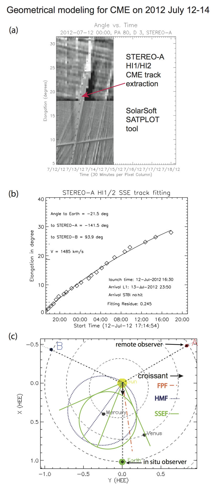
Figure 2.— Geometrical modeling of the 2012 July 12-14 CME. (a) The density track of the CME visible in a J-map from STEREO-A, with extracted time and elongation data points (“x” symbols) of the CME front, using the SATPLOT software tool available in IDL SolarSoft. (b) Fit of the extracted CME track with the Self-Similar Expansion Fitting (SSEF) model. Some results are indicated on the plot. Note that the Fixed-$\Phi$ Fitting (FPF) and Harmonic Mean Fitting (HMF) models (not shown) also reproduce well the observed time-elongation track. (c) The resulting geometry of the event, with propagation directions derived from FPF (dot-dashed red line emanating from the Sun), SSEF (solid green line) and HMF (dotted blue line) indicated. The HMF circle (180^∘ full width) is dotted blue, and the SSEF circle (90^∘ full width) is solid green. Also indicated is the direction from the croissant modeling by a black arrow.

2.3. In situ solar wind data

Figure 3 presents an overview of the near-Earth (L1) in situ solar wind data of proton bulk parameters and magnetic field components from 2012 July 13–18. We show data from the Solar Wind Experiment (SWE, Ogilvie et al., 1995) and the Magnetic Field Investigation (MFI, Lepping et al., 1995) on the Wind spacecraft, at a 1-minute time resolution. For 5 of the 24 in situ ICME arrivals in our study we use magnetic fields and proton data from the IMPACT (Luhmann et al., 2008) and PLASTIC (Galvin et al., 2008) instruments on the STEREO-B spacecraft.

In Figure 3 we can see the signatures of an ICME in the near-Earth solar wind. A clear shock is seen on 2012 July 14 1738 UT, signaled by sudden jumps in magnetic field, speed, density and temperature, delimited by the first solid vertical line on the left. Behind the shock follows the sheath region of high density and high temperature solar wind, and variable magnetic field. Around 2012 July 15 0600 UT, at the second solid vertical line, this region ends and the interval of a magnetic cloud (Burlaga et al., 1981) begins, which extends about 48 hours up to early July 17, where a third vertical line signals the end of the cloud. This region is an example of a clean magnetic structure passing the spacecraft, and is characterized by strong magnetic field strength, a smooth rotation of the magnetic field vector, which is shown in Geocentric Solar Ecliptic (GSE) coordinates, and low proton temperature. Such observations are usually interpreted as a magnetic flux rope, extending tube-like from the Sun with a helical magnetic field geometry (e.g. Al-Haddad et al., 2013; Janvier et al., 2013). We do not discuss magnetic cloud geometry further in this paper, but, for completeness, in this case the field rotates from solar east ($B_{Y}>0$) to south of the ecliptic ($B_{Z}<0$) to solar west ($B_{Y}<0$). This cloud is of east-south-west (ESW) type (Bothmer & Schwenn, 1998; Mulligan et al., 1998), and its axis is consequently roughly normal to the ecliptic plane pointing southward. Also shown are the results for arrival times and speeds by the geometrical modeling methods (“SSEF corr.” will be explained in Section 3.2). The fact that they are accurate to within a few hours of the observed arrival time at the location of Earth establishes the connection from the remote HI data to the in situ data near 1 AU.

In Table 2, columns 5–9, we present in situ results for every ICME event in our dataset, derived from similar plots. These parameters are: (column 5) the arrival time $t_{\mathrm{insitu}}$ of the shock, or, if no shock is present, the arrival time of a significant jump in proton density, (6) the average proton bulk speed $V_{\mathrm{sheath}}$ inside the sheath region, and its standard deviation, (7) the average proton density $N_{\mathrm{sheath}}$ inside the sheath, and its standard deviation, (8) the maximum magnetic field $B_{{\mathrm{max}}}$ in the full ICME interval (consisting of shock, sheath, and any magnetic structure), (9) the minimum value of the southward component of the magnetic field (min $B_{Z}$) in the full ICME interval. Some of these parameters act as an independent check on the validity of the results of the HI models, and highlight differences between the datasets when connecting CME observations from the Sun to 1 AU.

For this comparison, most relevant are the average proton bulk speed inside the ICME sheath region and the arrival time of the shock. The reason that we choose these parameters is that previous research has shown that the density, which is mapped by the HI instrument, and which shows up as a high density “track” in J-maps, corresponds to the region of enhanced plasma density in the ICME sheath (e.g. Rouillard et al., 2009; Möstl et al., 2009b, 2010; Lynch et al., 2010; Liu et al., 2011; Howard & DeForest, 2012a). Thus, tracking the leading edge of a CME in a J-map essentially means tracking the front of the sheath region, which is the location of the shock. Hence, the predicted arrival time from geometrical modeling corresponds to the shock arrival time observed in situ, and $V_{\mathrm{IPo}}$ corresponds to $V_{\mathrm{sheath}}$.

These in situ parameters are excellently suitable to act as target values for understanding the performance and limitations of the geometrical models, because they are very well defined, and have very small intrinsic errors. The arrival time of the shock can be pinpointed usually to within a few minutes accuracy, which is negligible when compared to the several hour error in arrival time prediction. For very slow ($\approx 400~{}$km s^-1) CMEs, where no shock is usually present, the in situ arrival time can be defined by the start of a high density region in front of the magnetic structure, to an uncertainty of $\pm 5$ hours. This definition was necessary only for the events with numbers 4 and 10 in our list. The speed $V_{\mathrm{sheath}}$ (column 6 in Table 2) has an average standard deviation of $\pm 23$ km s^-1. This is only 5% of the average sheath speed of 485 km s^-1, so it is also a well constrained quantity.

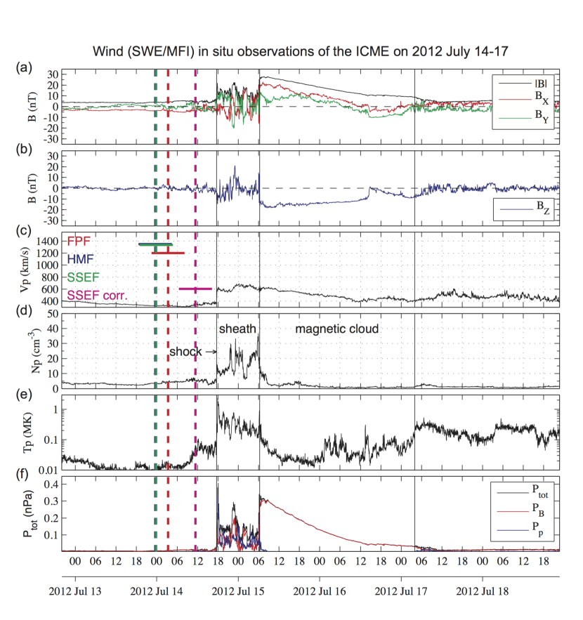
Figure 3.— In situ solar wind observations from the near-Earth Wind spacecraft, at the Sun-Earth L1 point, between 2012 July 13–18. From top to bottom: (a) Total magnetic field strength and $B_{X}$ and $B_{Y}$ components (in Geocentric Solar Ecliptic or GSE coordinates). (b) Magnetic field component $B_{Z}$ in GSE. (c) Proton bulk speed. (d) Proton number density. (e) Proton temperature. (f) Magnetic ($P_{B}$), plasma ($P_{\mathrm{p}}$) and total pressure ($P_{\mathrm{tot}}$). Predicted arrival times from the FPF (red), HMF (blue) and SSEF (green) models are indicated as vertical dashed lines. The speeds predicted by the same models are shown in panel (c) as horizontal bars, in similar colors, for direct comparison to the in situ proton bulk speed. The width of the horizontal bars corresponds to the estimated error in arrival time resulting from the manual selection of points ($\pm 10$% of the total CME transit time). The corrected arrival time (in version 1, see text) and the corrected speed (“SSEF corr.”) from section 3.2 are shown as pink vertical and horizontal lines, respectively.

3. Results

In this section, we discuss the results from an analysis of all the parameters that we described in the previous section for the full set of 22 different CME events. For the 2008 June 1–7 CME, there are two tracks in HI, one for the leading and one for the trailing edge, enveloping a magnetic flux rope (Möstl et al., 2009b; Lynch et al., 2010), thus we have two HI/in situ comparisons for a single CME. Additionally, for the CME on 2010 August 1–4, in situ data are available from the Wind and STEREO-B spacecraft, which observed different parts of the same shock front associated with the fastest and largest of several CMEs launched on the Sun on 2010 August 1 (Liu et al., 2012; Harrison et al., 2012; Möstl et al., 2012; Webb et al., 2013). In total, we end up with 24 different comparisons of imaging to in situ data. To track CMEs in HI data, we use STEREO-A for 21 events and STEREO-B for 1 event because of the slightly higher image quality for STEREO-A and some data gaps for STEREO-B. The imaging parameters are summarized in Table 1, and the in situ parameters are given in Table 2.

3.1. Connecting coronagraph to HI data

In this section, we discuss the comparison between CME parameters derived from the different imaging methods of croissant and geometrical modeling (Table 1). Essentially, we look for consistency between the CME speed and direction in the outer corona ($<15~{}R_{\odot}$ or 0.07 AU) and in the interplanetary medium (roughly up to 0.85 AU, see section 3.2.2 for details on the distance range). The initial directions and speeds of the CMEs are very well defined in the corona, as they are constrained by multi-view point imaging; this serves as a point of reference.

3.1.1 CME directions

Figure 4a shows the initial directions $\Phi_{\mathrm{init;Earth}}$ in the solar equatorial plane of all CMEs in our dataset, with the length of the arrow refering to the initial speed, both derived from the croissant model. In the time between the first event in 2008 April and the last event in 2012 July, STEREO-A separated itself from Earth from 25^∘ to 120^∘. It can be seen that for our specific set of events, the fastest CMEs tended to be launched about 30^∘ east and west of Earth, and only a few events were initially directed centrally toward Earth.

Figure 4b illustrates the interplanetary directions from SSEF modeling ($\Phi_{\mathrm{IP;HI}}$), relative to the HI observer, which is at the fixed longitude of 0^∘. The length of the arrow corresponds to the interplanetary speed of the SSEF circle’s apex ($V_{\mathrm{IP}}$). This figure demonstrates the important point that the fastest CMEs in our dataset were all backsided from the vantage point of the HI observer, and that the slow events were mainly frontsided. This is simply a consequence of the weak solar cycle 24, which resulted in CMEs which had well over 1000 km s^-1 only after the end of 2011. By this time, the two STEREO spacecraft had already reached a mutual separation greater than 180^∘ .

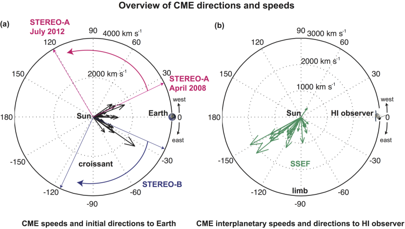
Figure 4.— (a) CME initial directions ($\Phi_{\mathrm{init}}$) in the solar equatorial plane, with respect to Earth (at 0^∘ longitude). The length of each arrow indicates the CME initial speed ($V_{\mathrm{init}}$). Both values are derived from croissant modeling, for a distance range $2.5-15~{}R_{\odot}$. (b) CME interplanetary directions ($\Phi_{\mathrm{IP}}$) from the SSEF model, in planes close to the solar equatorial plane, visualized with respect to the HI observer, which is STEREO-A for all but one event, explaining the bias towards solar east. The arrow length indicates the interplanetary CME speed ($V_{\mathrm{IP}}$) derived from SSEF modeling. It can be seen that for most of the fast CMEs the SSEF models yields backsided directions.

Figure 5 compares the CME directions from croissant modeling, $\Phi_{\mathrm{init;Earth}}$, to those from each geometrical model, $\Phi_{\mathrm{IP;Earth}}$. Each panel presents an angular histogram of $\Delta\Phi=\Phi_{\mathrm{IP;Earth}}-\Phi_{\mathrm{init;Earth}}$ with bins of 15^∘ width; $\Phi_{\mathrm{init;Earth}}$ is at 0^∘ longitude. The black arrow is the average $<\Delta\Phi>$. There is considerable scatter; as an example, 90% of interplanetary directions given by FPF are within $\pm 35$^∘ of the croissant direction.

The black arrow on each histogram shows that, on average, the croissant direction is consistent with FPF modeling to within a few degrees, whereas for the SSEF and HMF models, there is a bias in direction which increases with larger CME width. It results in an average difference in 30^∘ longitude between croissant and HMF directions. Because almost all events are observed by STEREO-A, which is positioned to the west of Earth and looks towards solar east, the resulting direction bias is towards solar east or angles $<0$^∘. This means that the SSEF and HMF methods places the CME apex further away from the HI observer. Lugaz & Kintner (2013) showed theoretically that this behaviour ultimately results from the constant speed assumption of the models, because the real deceleration of a fast CME in the interplanetary medium is interpreted by the models as geometrical deceleration, which means a change in direction as compared to a CME which is not decelerating. Lugaz & Kintner (2013) argued that the FPF model is in this way superior to the others, because the error resulting from neglecting deceleration is cancelled by neglecting the CME width.

We confirm this relationship from the observations in our dataset in Figure 6, where we plot the interplanetary speed $V_{\mathrm{IP}}$ against the difference in direction from the two extreme models FPF and HMF: $\Delta\Phi^{\prime}_{\mathrm{IP}}=\Phi_{\mathrm{IP;FPF}}-\Phi_{\mathrm{IP;HMF}}$. Higher interplanetary speeds are clearly correlated with larger differences in direction. We also quote linear relationships on the plot from which the resulting FPF–HMF direction difference $\Delta\Phi^{\prime}_{\mathrm{IP}}$ can be estimated, if $V_{\mathrm{IP}}$ is already known from one of the geometrical models.

We can take away from this section that connecting CME directions from the corona to the interplanetary medium works to within 30^∘ in heliocentric longitude. However, the models that feature an extended CME width (SSEF and HMF) and which are at first glance more mature than the point-like FPF model, produce systematically biased directions for fast CMEs.

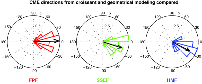
Figure 5.— A comparison of CME propagation directions in heliocentric longitude, from croissant modeling ($\Phi_{\mathrm{init;Earth}}$) and geometrical modeling ($\Phi_{\mathrm{IP;Earth}}$) for, from left to right, FPF, SSEF, and HMF. For each CME, the difference ($\Delta\Phi=\Phi_{\mathrm{IP;Earth}}-\Phi_{\mathrm{init;Earth}}$) is calculated, and the histogram of resulting angular differences is presented in bins of 15^∘ width. The direction of 0^∘ thus represents the croissant direction ($\Phi_{\mathrm{init;Earth}}$) in each panel. The black arrows show the mean of the direction difference. As the assumed width of the CME in the models rises from left to right, the difference in direction between the croissant and geometrical model increases, in the direction away from the imaging observer.

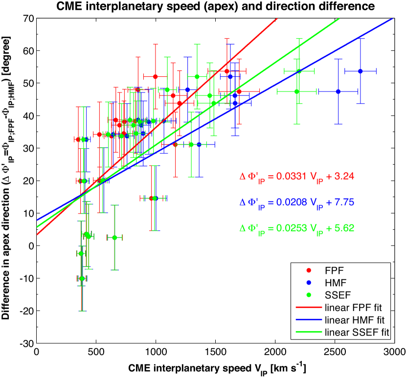
Figure 6.— CME interplanetary speed $V_{\mathrm{IP}}$ versus difference in heliocentric longitude of CME propagation directions between the FPF and HMF methods: $\Delta\Phi^{\prime}_{\mathrm{IP}}=\Phi_{\mathrm{IP;FPF}}-\Phi_{\mathrm{IP;HMF}}$. For each event, $\Delta\Phi^{\prime}_{\mathrm{IP}}$ is plotted against $V_{\mathrm{IP}}$ of all three methods (FPF, HMF, SSEF), and separate linear fits are performed for each method, with the resulting relationships quoted on the figure.

3.1.2 CME speeds and launch times

Figure 7 plots the relationship between the initial ($V_{\mathrm{init}}$) and the interplanetary ($V_{\mathrm{IP}}$) CME speed of the model apex. For each $V_{\mathrm{init}}$, the three different speeds by the geometrical models are shown. The black dashed line indicates where $V_{\mathrm{init}}=V_{\mathrm{IP}}$. We linearly fitted the data for each geometrical model separately. These linear fits work well for this relationship, and they allow one speed to be estimated if the other is known. They result in:

$$V^{\prime}_{\mathrm{IP}}=0.595\;V_{\mathrm{init}}+277,~{}~{}~{}~{}(\text{FPF model})$$ (1)

$$V^{\prime}_{\mathrm{IP}}=1.073\;V_{\mathrm{init}}+100,~{}~{}~{}~{}(\text{HMF model})$$ (2)

$$V^{\prime}_{\mathrm{IP}}=0.861\;V_{\mathrm{init}}+188,~{}~{}~{}~{}(\text{SSEF model})$$ (3)

with both speeds in km s^-1.

The FPF method yields a deceleration between the corona and the interplanetary medium (IP), with the slope of the linear fit indicating $V_{\mathrm{IP}}\propto 0.6~{}V_{\mathrm{init}}$. When using SSEF, the deceleration is less ($V_{\mathrm{IP}}\propto 0.86~{}V_{\mathrm{init}}$), and for HMF, the speed remains approximately constant, $V_{\mathrm{IP}}\propto 1.07~{}V_{\mathrm{init}}$. Here, again, our physical interpretation depends highly on which models we use, and thus these relationships are most useful for understanding the biases inherent in the different techniques. Nevertheless, taking these results at face value and knowing from theoretical considerations (Lugaz & Kintner, 2013) that FPF should give more accurate results for fast CMEs, a deceleration of CMEs from the corona to the IP medium seems to be the most realistic conclusion.

Furthermore, concerning another quantitative link between the COR2 and HI data sets, we checked whether the launch time $t_{0}$ resulting from the geometrical models is consistent with the time $t_{COR2}$ (see Table 1) of the first image of the CME in COR2. The launch time is defined as the time when the fitting function $\epsilon(t_{0})=0$ (Möstl et al., 2011). The average difference $<|t_{COR2}-t_{0}|>=1.7$ hours, and for $92\%$ of all events it is $<3~{}$hours. This means that the launch time is an excellent proxy for linking a CME track, which was extracted and from HI J-maps and modeled, to its coronal counterpart, provided that only one CME is launched during this time window.

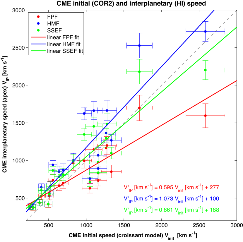
Figure 7.— Comparison between CME initial speeds $V_{\mathrm{init}}$, as derived from croissant modeling, and interplanetary propagation speeds. For each CME and its initial speed, the corresponding speed derived from the three geometrical models (FPF, HMF, SSEF) is plotted. The results of linear fits for all three models (red solid line for FPF, blue for HMF, and green for SSEF) are quoted with the corresponding colors.

3.2. Connecting HI to in situ data

In this section we discuss the link between the ICME in situ data and the speeds and arrival times derived from the HI observations. The CME direction cannot be compared to in situ because there is no simple way to derive the principal direction of an ICME from in situ data. This might be possible with deeper investigations on orientations of the shocks and flux ropes inside the ICMEs (e.g. Liu et al., 2010b; Möstl et al., 2012; Isavnin et al., 2013), but this is beyond the scope of the current study.

3.2.1 CME and ICME speeds

We first focus on a comparison of speeds. For the heliospheric imager data, these are the speeds toward the in situ observer ($V_{\mathrm{IPo}}$) derived from the three geometrical models (FPF, HMF, SSEF). For the in situ ICME data, these are the average proton bulk speeds in the ICME sheath regions ($V_{\mathrm{sheath}}$).

Figure 8 shows the difference $\Delta V=V_{\mathrm{IPo}}-V_{\mathrm{sheath}}$ for each event included in our study. Note that the speed $V_{\mathrm{IPo}}$ already includes a correction to account for which part of the CME front impacts the spacecraft. It is clearly seen that for most slow CMEs in the sample, until late 2011, there is a relatively good consistency. For FPF, in 42 % of events the absolute difference $|\Delta V|<200$ km s^-1 (SSEF: 54 %; HMF: 50%). This means that for about half of the events there is a reasonable match between the imaging and in situ speeds.

However, most IP speeds exceed the in situ ones. For FPF, 87 % of events are faster in the IP medium than when observed in situ (SSEF: 75 %, HMF 83 %). This is most evident for the fast CMEs in our sample, those with initial speeds $>1000$ km s^-1, for which the predicted in situ speeds are strongly overestimated (consistent with Lugaz & Kintner, 2013), on the order of 500 to 1000 km s^-1. These are the events on the right side of Figure 8. The geometrical models yield an average interplanetary propagation speed of a CME. Especially for very fast CMEs, these speeds will not match the speeds measured in situ at 1 AU because of the CME deceleration that occurs up to 1 AU (e.g. Gopalswamy et al., 2001; Vršnak et al., 2013). In essence, the assumption of constant speed in the geometrical models is at the root of this discrepancy.

Table 3 summarizes the $|\Delta V|$ obtained with the different methods. On average, $<|\Delta V|>$ is 303 km s^-1 (FPF), 267 km s^-1 (SSEF) and 282 km s^-1 (HMF). Taking the average over these values gives 284 km s^-1. We can also see that the differences between the geometrical models are only about 40 km s^-1, which makes it impossible to state which one performs best. In Table 3 we also state the results of a comparison $|\Delta V|=|V_{\mathrm{IP}}-V_{\mathrm{sheath}}|$, which means that we just use the CME model apex speed without a correction for the position of the in situ observer. This results in an average difference over all models of 431 km s^-1. Consequently, correcting for apex or flank encounters strongly enhances the consistency with in situ data, for the present set of events on average by $\approx 150$ km s^-1. However, this is likely caused by the effect that a flank speed is invariably lower than the apex speed, simulating to some degree the effect of real CME deceleration. But even when using $V_{\mathrm{IPo}}$, the average difference to the in situ speeds is still too large, almost 300 km s^-1. It becomes clear that we need to introduce some kind of correction to the interplanetary speeds to be able to better predict the in situ speed from heliospheric images.

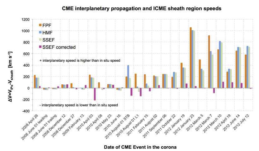
Figure 8.— Difference between the CME interplanetary speed in the direction of the in situ observatory ($V_{\mathrm{IPo}}$) and the ICME sheath speed ($V_{\mathrm{sheath}}$), for each model (FPF red, HMF blue, SSEF green), and for each CME event. The pink bars show the difference to $V_{\mathrm{sheath}}$ using the corrected speed $V^{\prime}_{{\mathrm{sheath}}}$ for SSEF modeling. The corrected speed is calculated by using the linear fit for SSEF as indicated on Figure 9.

Figure 9 presents the interplanetary speed ($V_{\mathrm{IPo}}$) in the direction of the in situ observatory against the ICME sheath region speed ($V_{\mathrm{sheath}}$). Separate linear fits for each geometrical model are shown in corresponding colors. These fits are very similar to each other. With the coefficients from these fits, we can apply an empirical correction to the speed $V_{\mathrm{IPo}}$ for each model, to get a better proxy for the speed of the in situ sheath region, which we call $V^{\prime}_{\mathrm{sheath}}$ or a “corrected” speed:

$$V^{\prime}_{\mathrm{sheath}}=0.227V_{\mathrm{IPo}}+307,~{}~{}~{}~{}(\text{FPF model})$$ (4)

$$V^{\prime}_{\mathrm{sheath}}=0.213V_{\mathrm{IPo}}+323,~{}~{}~{}~{}(\text{HMF model})$$ (5)

$$V^{\prime}_{\mathrm{sheath}}=0.205V_{\mathrm{IPo}}+334,~{}~{}~{}~{}(\text{SSEF model})$$ (6)

with both speeds given in km s^-1. We use this formula to obtain corrected sheath speeds based on $V_{\mathrm{IPo}}$, and compare them again to the in situ observed $V_{\mathrm{sheath}}$.

Returning to Figure 8, the pink bars show the comparison $\Delta V=V^{\prime}_{\mathrm{sheath}}-V_{\mathrm{sheath}}$, for the SSEF method only. It can be seen that the consistency with $V_{\mathrm{sheath}}$ greatly improves, for both slow and fast CMEs. On average, $<|\Delta V|>=50$ km s^-1 (FPF), 53 km s^-1 (SSEF) and 57 km s^-1 (HMF); see again Table 3 for a summary. For the whole dataset, for FPF, the absolute difference $|\Delta V|<100$ km s^-1 in 92 % of cases (SSEF: 83 %; HMF: 88%). This is an improvement over more than 200 km s^-1 compared to geometrical modeling without this empirical correction. Clearly, the caveat of this correction is that we derived it from the current set of events, and the results will change for a different set of CMEs. Nevertheless, it definitely results in an improvement in the prediction capability compared to using the geometrical models alone, and should also be used in future studies.

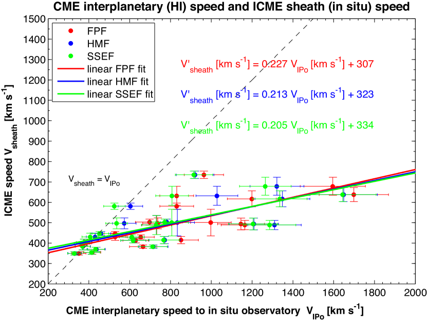
Figure 9.— Comparison between interplanetary CME speeds in the direction of the in situ observatory $V_{\mathrm{IPo}}$ (from geometrical modeling) and the observed proton bulk speeds $V_{\mathrm{sheath}}$ inside the ICME sheath regions. For each ICME, results for all three geometrical models are plotted (FPF red, HMF blue, SSEF green). Linear relationships derived for each of the three models are shown in the corresponding colors. The black dashed line indicates where the two speeds are equal.

In summary, the average difference between CME speeds predicted from geometrical modeling to in situ ICME sheath region speeds are, for all methods, using $V_{\mathrm{IP}}$, $<|\Delta V|>=431$ km s^-1; using $V_{\mathrm{IPo}}$, $<|\Delta V|>=284$ km s^-1, and using $V^{\prime}_{\mathrm{sheath}}$, $<|\Delta V|>=53$ km s^-1. The differences between the different geometricals model are negligible, so none can be claimed as performing significantly better than the other.

3.2.2 Interplanetary distance ranges

Before we move on to discuss similar comparisons of ICME arrival times, we first need to clearly state the range of distances in the interplanetary medium that are covered by the STEREO/HI observations. Using J-maps created by the SATPLOT software, we tracked every CME event out to about 30–40^∘ elongation from the Sun. Rather than elongation, we need to know the corresponding distance range in AU to see how far from the Sun we have actually tracked the front of each CME. The average elongation value of the last HI data point of each CME is $34.9\pm 7.1$^∘. The corresponding distance to the maximum elongation is calculated by $d_{\mathrm{p}}=(t_{\mathrm{p}}-t_{0})\times V_{\mathrm{IP}}$. This means that we propagate the CME away from the Sun with the interplanetary speed of the model apex, from the launch time to the last time of HI observation ($t_{\mathrm{p}}$). For simplicity, we state the result as a mean and standard deviation for all CMEs for the SSEF model only, because it is intermediate between the FPF and HMF models. The average maximum distance of the CME apex from the Sun, over all CMEs, is $<d_{\mathrm{p}}>=0.855\pm 0.276$ AU (SSEF). The maximum value is 1.41 AU, and the minimum 0.48 AU. The maximum apex distance for some events is $>1$ AU, especially for those cases where the CME flank hits the in situ spacecraft, which is situated near 1 AU.

3.2.3 Prediction lead times

We focus on connecting CMEs in different datasets, so we track the CMEs in the HI data for as long as possible. But we can also ask ourselves how useful the results will be for forecasting the in situ parameters. For this it is necessary to place the parameters that we have calculated from remote images, and their comparison to in situ observations, into the context of space weather prediction.

A very important parameter in this respect is the prediction lead time ($t_{\mathrm{lead}}$). This is the difference between the actual in situ arrival time of the ICME, and the time ($t_{\mathrm{p}}$) when a prediction for its arrival was issued. In our study, the latter is again the last point at which the event was observed by HI (i.e., the last point clicked in a J-map); of course here we are not discussing real time predictions but artificial “predictions” made long after the events have happened, derived from a pre-existing dataset. We define $t_{\mathrm{lead}}=t_{\mathrm{p}}-t_{\mathrm{insitu}}$, where $t_{\mathrm{insitu}}$ is the actual ICME arrival time. With this definition, prediction times earlier than the actual arrival give a $t_{\mathrm{lead}}<0$, as desirable when really “predicting” CMEs. Over our dataset, on average, $<t_{\mathrm{lead}}>=-26.4\pm 15.3$ hours, with a minimum $t_{\mathrm{lead}}$ for any individual event of $-53.6$ hours ($>2$ days), and a maximum of $+0,28$h. For the latter, $t_{p}$ was already later than the in situ arrival time. Hence, the results that we state for arrival times and speeds are valid for a prediction lead time of the order of one day, albeit with considerable scatter around this value. We also need to point out that we have used HI science data, which are of better quality than those available from STEREO in real time.

3.2.4 Arrival times

Figure 10 is a bar chart showing, for all CMEs, the difference $\Delta t=t_{\mathrm{a}}-t_{\mathrm{insitu}}$ between predicted CME arrival time and the observed ICME arrival time taken from the in situ measurements. Here, $t_{\mathrm{a}}$ is the predicted arrival time from heliospheric imaging, derived by the following expression (similar to Möstl et al., 2011; Möstl & Davies, 2013),

$$t_{\mathrm{a}}=t_{0}+\frac{d_{\mathrm{i}}}{V_{\mathrm{IPo}}},$$ (7)

where $t_{0}$ is the launch time, as discussed above, $d_{\mathrm{i}}$ is the heliocentric distance of the in situ spacecraft, and $V_{\mathrm{IPo}}$ the (assumed constant) CME speed in the direction of the in situ observatory.

In Figure 10, values of $\Delta t<0$ refer to the situation where the predicted arrival time is before the in situ arrival time. This is the case in particular for the events after October 2011, on the right hand side of Figure 10, which are all backsided events, from the HI observer point of view, as determined by the SSEF direction. Even so, the fastest CMEs after October 2011 have a reasonable $|\Delta t|<10$ h, but this is mainly due to the fact that fast CMEs have a transit time of the order of 20–40 hours, compared to around 100 hours for slower events. In general, we find $\Delta t$ is of the order of 10% of the total CME transit time. However, all three methods predict arrival times that are one day early for slow and backsided CMEs (e.g. 2012 April 19 with $V_{\mathrm{init}}=639$ km s^-1), consistent with theoretical expectations (Lugaz & Kintner, 2013).

There is considerable scatter around $\Delta t\approx 0$, and for a specific event, different methods can give quite different arrival times. The maximum and minimum values of $\Delta t$ are about $\pm 1$ day, while the average absolute values of $<|\Delta t|>=8.5\pm 5.4$h for the FPF model (SSEF: $8.4\pm 7.2$h; HMF: $7.5\pm 6.6$h; $8.1\pm 6.3$h over all methods). Results are summarized in Table 3, including averages of signed values of $<\Delta t>$.

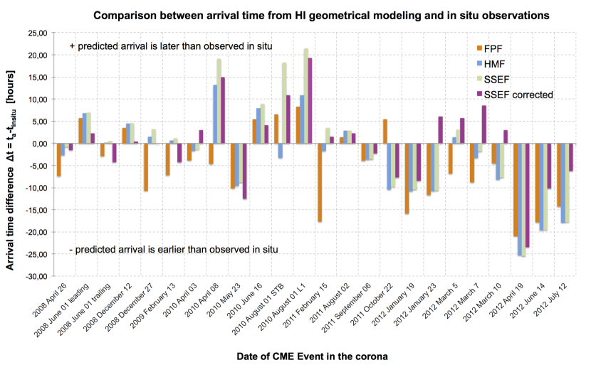
Figure 10.— Difference between CME arrival time as derived from geometrical modeling and actual ICME arrival time at the in situ observatory, for each CME event and each geometrical model (FPF: red; HMF: blue; SSEF: green). Pink bars indicate differences between corrected arrival times and the observed in situ arrivals ($\Delta t=t_{a;corr;v1}-t_{insitu}$). The corrected arrival times (for SSEF only) were calculated with the linear relationship shown in Figure 11.

We have derived corrections to the arrival times, using a similar approach as for correcting the speed predictions, but independent of the results for the speeds. Figure 11 is a scatter plot of the interplanetary speed $V_{\mathrm{IPo}}$ versus $\Delta t$, for each CME and for all three methods. Faster interplanetary speeds tend to be correlated with lower values of $\Delta t$, attributable again to the constant speed assumption used in geometrical modeling. Faster CMEs are predicted to arrive before they actually do, because modeling a fast and decelerating CME assuming a constant speed results in a much higher speed than the final in situ speed, as we have shown in the previous section. Similar to what was done in Figure 9, we fit the data points in Figure 11 for each model independently with a simple, linear relationship. The results of these fits are:

$$\Delta t^{\prime}=-0.0078V_{\mathrm{IPo}}-0.52~{}~{}~{}(\text{FPF model}),$$ (8)

$$\Delta t^{\prime}=-0.0144V_{\mathrm{IPo}}+7.64~{}~{}~{}(\text{HMF model}),$$ (9)

$$\Delta t^{\prime}=-0.0169V_{\mathrm{IPo}}+11.04~{}~{}~{}(\text{SSEF model}),$$ (10)

with $\Delta t^{\prime}$ in hours and $V_{\mathrm{IPo}}$ in km s^-1. This allows to make an empirical correction (that we call “version 1”) to the arrival time from our knowledge of $V_{\mathrm{IPo}}$ alone. To this end, we calculate a corrected arrival time by

$$t_{\mathrm{a;corr;v1}}=t_{\mathrm{a}}-\Delta t^{\prime},$$ (11)

using $\Delta t^{\prime}$ from the fit for the corresponding geometrical model. The result of such a calculation for the SSEF model is shown using pink bars in Figure 10. On average, it improves the prediction performance by 2 hours. Comparing corrected arrival times to in situ arrival times results in $<|\Delta t|>=5.6\pm 4.1$h for the FPF model (SSEF: $6.8\pm 6.0$h; HMF: $5.9\pm 4.9$h). The average over all models is $6.1\pm 5.0$h, compared to 8.1 hours without the empirical correction (see Table 3).

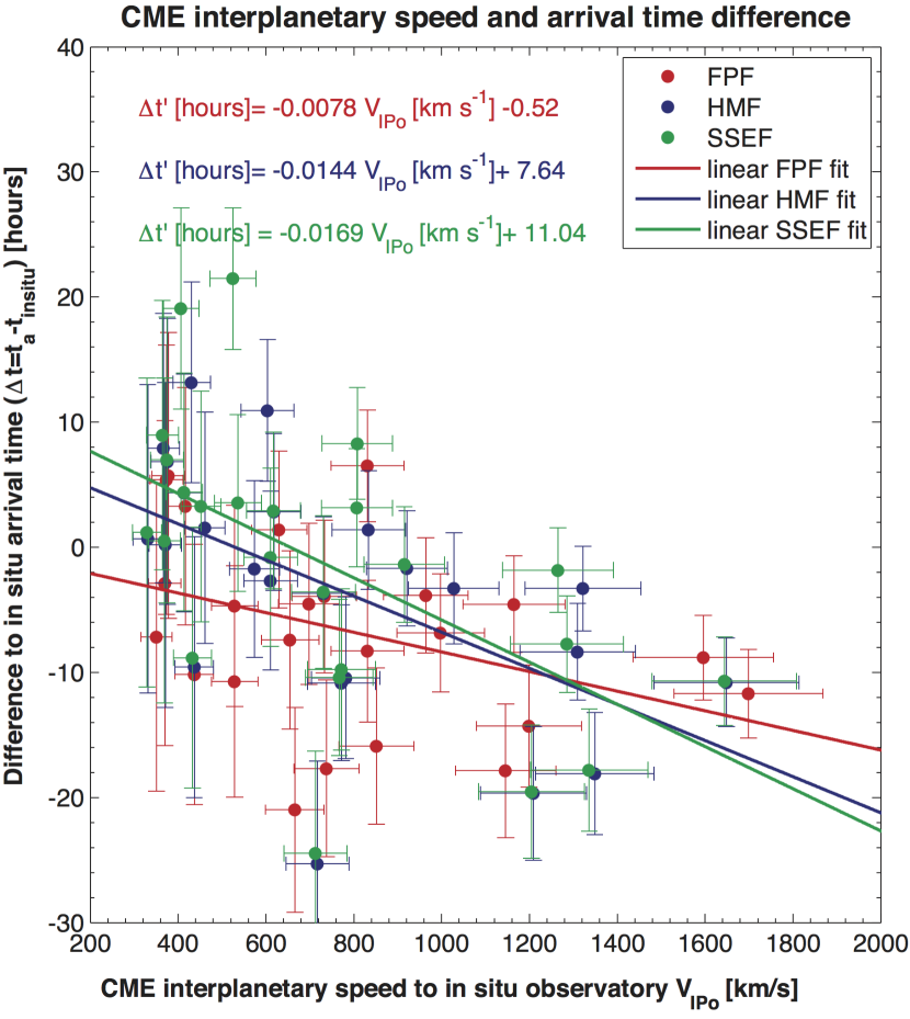
Figure 11.— Scatter plot of the difference between observed in situ ICME arrival times and predicted arrival times from geometrical modeling. Linear fits are shown as solid lines: FPF (red), HMF (blue), SSEF (green). Corresponding relationships are quoted on the figure in the respective color.

3.2.5 Transit times

There is another way to calculate CME arrival times which performs slightly better than the straightforward arrival time calculation using geometrical modeling, as stated in Equation (7). We have applied this new method, that we call “version 2”, which also depends only on $V_{\mathrm{IPo}}$, to our list of events. We define a CME’s transit time $TT$ as the time difference between its first appearance in coronagraph images ($t_{\mathrm{COR2}}$), and its actual in situ arrival time $t_{\mathrm{insitu}}$. This definition of $TT$ covers a distance range from $2.5~{}R_{\odot}$, which is the inner boundary of STEREO/COR2, to 1 AU or $\approx 215~{}R_{\odot}$.

Figure 12 shows a relationship between $TT$ and interplanetary speeds ($V_{\mathrm{IPo}}$) for all CMEs in our dataset. For each geometrical model, we fit a power law to the data, quoting the results on the plot. For SSEF, the resulting power law is:

$$TT^{\prime}=9537\times V_{\mathrm{IPo}}^{-0.76}~{}~{}~{}~{}(\text{SSEF model},)$$ (12)

with $V_{\mathrm{IPo}}$ given in km s^-1, and $TT^{\prime}$ in hours. Similar relationships have been shown for example by Schwenn et al. (2005) and Vršnak & Žic (2007), but using CME coronagraph speeds, whereas we show interplanetary speeds. They include to some extent the CME propagation through the background solar wind. The average transit time in our dataset is around 72 hours (or 3 days), which compares well to the classic Brueckner et al. (1998) 80 hour rule for average CME transit times. These power laws allow us to predict the arrival time, based solely on the interplanetary speed in direction of the in situ observatory $V_{\mathrm{IPo}}$, by

$$t_{\mathrm{a;corr;v2}}=t_{0}+TT^{\prime}.$$ (13)

For simplicity, we do not show resulting arrival time differences $\Delta t$ for each event, but only summarize the resulting values. For this method, the difference between predicted and in situ arrival times is $<|\Delta t|>=5.7\pm 3.8$h for the FPF model (SSEF: $7.7\pm 6.1$h; HMF: $6.6\pm 5.3$h). The average for all models is $6.6\pm 5.1$ hours, almost as good as for the empirically corrected arrival times (6.1 hours).

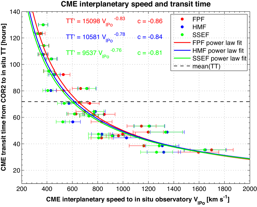
Figure 12.— CME interplanetary propagation speeds $V_{\mathrm{IPo}}$, in the direction of the in situ observatory, plotted against CME transit times $TT$. For each event, $V_{\mathrm{IPo}}$ from each of the three geometrical models are given: FPF (red), HMF (blue), and SSEF (green). Power law fits for each model are plotted as solid lines, with the function and the correlation coefficent ($c$) for each method quoted on the image. The black dashed line shows the mean transit time for the CMEs in our sample, $<TT>=71.9$ hours.

3.2.6 CME speed and ICME magnetic field

The last step in our analysis concerns the relationship between the maximum magnetic field $B_{\mathrm{max}}$ in the full ICME interval (column 8 in Table 2), consisting of shock, sheath and ejecta parts, and the interplanetary speed $V_{\mathrm{IPo}}$ in the direction of the in situ observatory, as derived from HI geometrical modeling. CMEs that have higher speeds close to the Sun are known to be correlated with stronger magnetic fields at in situ spacecraft (e.g. Lindsay et al., 1999; Yurchyshyn et al., 2005). This is thought to arise from the role played by magnetic reconnection during CME eruption, namely through a possible formation of their interior magnetic flux rope (e.g. Qiu & Yurchyshyn, 2005; Qiu et al., 2007; Möstl et al., 2009c). Another explanation is that faster CMEs lead to stronger compression of the ambient solar wind, which results in a higher magnetic field strength in the ICME sheath region (Liu et al., 2008). Around half of the ICMEs in our dataset reach their $B_{\mathrm{max}}$ in the sheath and the other half in their interior magnetic ejecta, so both effects can be expected to play a role in our analysis. In the same way as we have done for the transit times above, we can extend such previously found relationships by comparing interplanetary rather than coronal CME speeds to the in situ magnetic field magnitude.

Figure 13 shows, as a scatter plot, that stronger ICME maximum magnetic fields are correlated with faster interplanetary CME speeds. Again, we perform independent, linear fits for each model, which, for SSEF, results in

$$B^{\prime}_{\mathrm{max}}=0.0189V_{\mathrm{IPo}}+6.73,$$ (14)

with $B_{\mathrm{max}}^{\prime}$ in nT, and $V_{\mathrm{IPo}}$ in km s^-1. The average, absolute difference $\Delta B=B^{\prime}_{\mathrm{max}}-B_{\mathrm{max}}$ between predicted and observed maximum magnetic fields, based on the speeds from FPF, is $<|\Delta B|>=4.8$ nT (SSEF: 4.7 nT; HMF: 4.4 nT). Use of the resulting linear fits for $B_{max}^{\prime}$ for each model results in a successful prediction of $B_{\mathrm{max}}$ to within $\pm 5$ nT for 58 % of events with the FPF method (SSEF: 67%; HMF 71%). The same numbers for predictions within $\pm 10$ nT are 88 % for FPF (SSEF: 88%; HMF 92%). In summary, for around 2 out of 3 events in our sample, the maximum magnetic field in the ICME interval could be predicted within a precision of 5 nT, solely based on the interplanetary CME speed.

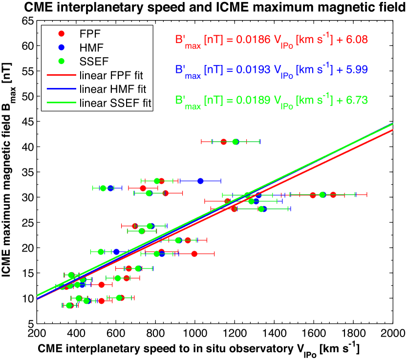
Figure 13.— Relationship between the in situ observed maximum magnetic field $B_{max}$ in the full ICME interval (shock, sheath, and ejecta) and the interplanetary CME speed in direction of the in situ observer ($V_{\mathrm{IPo}}$). Formulas for linear fits to the data, for each model, are given in corresponding colors.

4. Conclusions

We have presented a study in which we have connected white light to in situ observations of a set of 22 near-equatorial CMEs. Their parameters cover a wide range of initial and propagation speeds (260 to 2715 km s^-1), and a variety of principal CME directions with respect to the HI observer (40^∘ to 170^∘ in heliocentric longitude). This is the first study to do such an analysis of such a large and diverse set of events. Here, we summarize our results and their implication for space weather prediction and the evolution of CMEs between the Sun and 1 AU separately, emphasizing our main conclusions in italics.

First, concerning space weather prediction, we have mainly tested methods for predicting CME directions, speeds and arrival times based on J-maps produced using observations from a single-spacecraft heliospheric imager instrument. These data were provided by HI on STEREO-A/B, which, for the CMEs under study, were positioned well outside the Sun-Earth line, on heliocentric longitudes between 30^∘ and 120^∘ away from the Earth.

1. Event selection: We have selected CME events with clear interplanetary CME signatures (shock, sheath and ejecta) in Wind and STEREO-B in situ observations near 1 AU, and which we could easily track in the HI J-maps. This set of CMEs covers a wide range of initial speeds, so it is suitable for statistical analysis, although there are actually many more CMEs in the data during this time range. The events in our list occurred during the rise of solar cycle 24, between 2008-2012, and STEREO progressed towards and beyond opposition during this time. Therefore, our dataset contains mostly slow frontsided and fast backsided CMEs. Our results must be considered carefully with this in mind, and are likely to be different for different datasets.

2. Tracking CMEs and prediction lead times: We tracked CMEs as far as possible in the J–maps, resulting in an average track length of $34.9\pm 7.1$^∘ elongation. Depending on the CME speed, its direction and the model applied, this corresponds to different distances each CME has traveled away from the Sun at the time of the last HI observation. This distance is on average $0.86\pm 0.28$ AU, thus we have tracked most CMEs almost up to 1 AU. The prediction lead times also depend on several of the aforementioned parameters, and are on average $-26\pm 15$ hours, about $-1$ day. This is considerably longer than those provided by a solar wind monitor at L1 (on the order of 1 hour, e.g. the current ACE mission), but definitely shorter than lead times using corongraphs only (on the order of CME transit times of a few days, e.g. Kilpua et al., 2012). The work presented here should rather be seen as an attempt to establish connections between CME-related phenomena detected in different data sets (coronagraph, heliosphere, in situ), which is strongly desirable for benchmarking various empirical or numerical CME prediction models.

3. CME directions: The three different geometrical models used in this study do not provide consistent CME directions, with differences of up to 50^∘ in heliocentric longitude for fast CMEs. For this reason, we derived the direction from multi-viewpoint applications of the croissant model to coronagraph images as a well constrained reference for the initial CME direction. The FPF direction was shown to be, on average, consistent to within a few degrees with the croissant direction. This means that if CMEs propagate radially away from the Sun above 15 solar radii, the FPF method is superior over the others in deriving the CME principal direction. However, there is also considerable scatter, of the order of $\pm 30$^∘ heliocentric longitude around the average direction. The directions provided by the SSEF and HMF models, which assume an extended CME front, differ by about $30$^∘ from the croissant direction. These methods show a bias in the direction to values further away from the HI observer, with larger differences for faster CMEs, confirming theoretical predictions by Lugaz & Kintner (2013).

4. CME arrival time and speed predictions: Using geometrical modeling to predict CME speed and arrival time, with a lead time of roughly 1 day, results in average absolute differences from observed ICME sheath speeds and arrival times of $|\Delta V|=284\pm 288$ km s^-1 and $|\Delta t|=8.1\pm 6.3$h, respectively, averaged over all three methods. The arrival time difference given by the root-mean-square method is $\Delta t_{RMS}=10.3$h. Conserving the sign of the differences, similar numbers for calculated minus observed speeds and arrival times are $\Delta V=275\pm 297$ km s^-1 and $\Delta t=-3.8\pm 9.6$h, respectively. In summary, predicted ICME speeds at 1 AU are, on average, overestimated, and consequently, predicted arrival times are too early compared with the in situ observations. Correlating the interplanetary CME speed in the direction of the in situ observatory with the in situ speeds, and, independently, with the differences in observed and predicted arrival times, we obtained new empirical relationships between these variables, based on linear fits. These allow us to predict the CME speed and arrival time with better accuracy for, at least, the present dataset. Applying these empirical corrections in the prediction of CME speeds and arrival times, $|\Delta V|=53\pm 50$ km s^-1($\Delta V=0\pm 73$ km s^-1), and $|\Delta t|=6.1\pm 5.0$h ($\Delta t=0.0\pm 7.9$h, $\Delta t_{RMS}=7.9$h), averaged over all events and methods. More specifically, 88% (or roughly 9 out of 10) of all in situ ICME sheath region speeds in our dataset were predicted to within $|\Delta V|<100$ km s^-1. In 71% of cases (or roughly 3 out of 4), ICME arrival times are predicted within $|\Delta t|<8$ hours. Moreover, we quantified the relationship between the maximum magnetic field $B_{max}$ in the ICME and the interplanetary propagation speed, which lets us predict $B_{max}$ to within $\pm 5$ nT in 2 out of 3 cases.

5. Comparison to stereoscopic modeling: Colaninno et al. (2013) found similar results for CME arrival time and speed prediction using the results of methods applied to two heliospheric imager instruments, such as fitting the stereoscopic croissant model to STEREO/COR2/HI1/HI2 and SOHO/LASCO images, for heliocentric distances up to about 0.9 AU. Similar to our study, they also applied corrections for the apex and flank parts of the CMEs impacting the in situ observatory. They found that for 78% of cases, $\Delta t<6$ hours, and for 55% of CMEs, $\Delta V<100$ km s^-1, although for all events $\Delta V<140$ km s^-1. Colaninno et al. (2013) fitted the height-time data in several different ways, and they found a linear fit between $50$ $R_{\odot}$ (0.23 AU) and 1 AU and thus assuming a constant speed to produce the best predictions, even though they also concluded that CMEs clearly decelerate. It is interesting to note that an equivalent assumption of constant speed between 0.07 to 0.85 AU in our geometrical modeling methods yields a similar level of predictive performance.

Second, we summarize our results in terms of the physical evolution of CMEs between the Sun and 1 AU. In general, we find that, using single-spacecraft HI observations, it is much more difficult to generalise the behavior of CMEs in terms of such properties as propagation direction, speed variation and global shape evolution when compared to the use of stereoscopic HI measurements (e.g. Liu et al., 2010a; Lugaz et al., 2010; Liu et al., 2011; Colaninno et al., 2013; Mishra & Srivastava, 2013; Liu et al., 2013; Davies et al., 2013).

1. CME radial propagation: A major unsolved question is whether CMEs propagate radially away from the Sun, or undergo any significant change of direction as they travel through the interplanetary (IP) medium. CMEs are known to be deflected in the corona by coronal holes (Gopalswamy et al., 2009) and possibly through CME-CME interaction in IP space (Lugaz et al., 2012). Liu et al. (2013) and Davies et al. (2013) showed the CME direction for a few events to stay within about $\pm 15$^∘ (heliocentric longitude) from the corona to the IP medium. This can still be considered as consistent with a radial propagation. With our own dataset, CME deflections are difficult to assess without further analysis. As discussed above, the HI methods can give very different answers for a single event - CME principal directions are not well defined using single-spacecraft HI methods. Note also that we assume constant direction in IP space in contrast to the stereoscopic methods, so we can only assess deflections by comparing directions derived from coronagraph and HI measurements. However, there is considerable scatter between these initial and IP directions (of the order of $\pm 30$^∘, about twice the level derived from stereoscopic methods), pointing indeed to the possibility that some CMEs may significantly change in direction between the corona and the IP medium. While the croissant model constrains the CME direction well close to the Sun, there is no straightforward way to constrain the CME direction using single-spacecraft in situ data, and thus we leave further analysis for future work.

   Our results on CME direction in IP space clearly point out that its calculation is always influenced by the strongly idealized shapes of the CME front which we assume in the first place. The geometrical definitions we use make it possible to describe CME front shapes analytically, and form very useful tools. However, our study casts some doubts on their use in defining a CME’s central propagation direction in the interplanetary medium, because its calculation depends so strongly on the assumption of its frontal geometry. Consequently, we propose that future work should quote ranges of heliocentric longitude that will be affected by a CME, rather than a central direction. This would be especially helpful when describing distorted or asymmetric CME front shapes (e.g. Savani et al., 2010; Möstl et al., 2012).

2. CME speed profiles: CMEs are well known to decelerate in the solar wind out to 1 AU, mainly due to a force equivalent to aerodynamic drag (e.g. Gopalswamy et al., 2001; Kilpua et al., 2012; Vršnak et al., 2013; Liu et al., 2013), and we can see this clearly in our data. We can compare stepwise a CME initial speed ($<15~{}R_{\odot}$, or $<0.07$ AU) to its average IP propagation speed (from $\approx 0.07$ to $0.86\pm 0.28$ AU), and to the speed of the ICME sheath region observed in situ near 1 AU. FPF and SSEF suggest that CMEs decelerate from the corona to IP space, while HMF yields a constant speed. CMEs are clearly slower when observed in situ near 1 AU than in IP space, and the in situ sheath region speeds can be reasonably well predicted by multiplying the IP speeds with $\approx 0.2$ and adding $320$ km s^-1, which is independent of the model used. The speed of $320$ km s^-1 is reminiscent of the slow solar wind, and this relationship is also consistent with early work by Lindsay et al. (1999). However, we cannot definitely say where most of the deceleration occurs, because of our assumption of constant IP speed. Recent analyses with stereoscopic methods by Liu et al. (2013) showed that much of the deceleration of fast CMEs occuring up to about 80 solar radii (0.37 AU), but there is probably no general distance by which the deceleration ceases, as a case has been found where a CME almost does not decelerate out to 1 AU (Möstl et al., 2010).

3. Evolution of the global CME shape: We expected that there would be clear differences concerning the prediction performance of different geometrical models, giving us hints which one better describes the CME front shape in the plane perpendicular to the HI images. In particular, we expected the SSEF model, as it is the most mature, with a well defined CME width, to perform best. But surprisingly, we did not find any significant difference in its performance for predicting CMEs compared to the other models. We think that this is caused by their assumptions of constant speed and constant direction, and their high sensitivity to a violation of these assumptions (Lugaz & Kintner, 2013). In summary, the current state of the art of geometrical modeling of CMEs with single-spacecraft instruments (i.e. fitting methods) in comparison to single-spacecraft in situ data precludes inferences to be made regarding the large–scale geometry of CME fronts in planes perpendicular to the HI images, such as the ecliptic plane.

We conclude that predicting CME speeds and arrival times with heliospheric images gives more accurate results than using projected initial speeds from coronagraph measurements. These improvements are on the order of 12 hours for the arrival times (Colaninno et al., 2013), and our results are consistent with those found with other space weather models in the STEREO era (see also Gopalswamy et al., 2013; Mishra & Srivastava, 2013; Mishra et al., 2014). Independent of the specific methods used, we can derive an average of the CME interplanetary propagation speed when we track a CME out to 1 AU. This average speed includes to some extent the background solar wind, which is known to play a significant role in modulating CME propagation (e.g. Gopalswamy et al., 2001; Vršnak & Žic, 2007; Temmer et al., 2011; Kilpua et al., 2012). The same is true for interacting CMEs, although it can be very difficult to differentiate and decipher different density tracks in HI when CMEs are launched close together in time and space (Harrison et al., 2012; Webb et al., 2013).

It is clear that the information contained in heliospheric images does indeed improve space weather prediction. However, the compromise between prediction accuracy ($\Delta t$) and prediction lead times ($t_{lead}$) needs to be better studied. Future modeling should thus focus on modeling CME tracks in J-maps for elongations from the Sun of $<35$^∘, which will result in longer prediction lead times than one day in the current study. It needs to be assessed how the predictions for speed and arrival time become less accurate as the prediction lead time is increased, and the best balance for space weather prediction purposes needs to be found.

Another possibility for future work is to actually include deceleration into the geometrical fitting methods for single-spacecraft HI instruments. This is expected to further improve the accuracy of predicting CME arrival times and speeds through use of a more realistic approach than the current assumption of constant speed. Such an approach, applied to the different model geometries, could provide clues to the CME global front shape, in particular when constrained by multi-point in situ measurements.

Another solution would be to send a mission equipped with a heliospheric imager in a polar orbit around the Sun to look down onto the ecliptic plane (Liewer et al., 2008). In this way, information on the global shape of a CME in the ecliptic, as it approaches Earth, would be revealed, and the CME propagation characteristics could be provided by the geometrical models as used in our paper. However, for effectively predicting geo-effectiveness it is also necessary to know the components of the interplanetary magnetic field, which cannot be derived from white-light images, and require new ideas like the Faraday-rotation technique (e.g. Xiong et al., 2013b). Moreover, the Solar Orbiter (e.g. Müller et al., 2013) and Solar Probe Plus missions are currently under development and will approach the Sun closer than ever before by the end of the decade. The results and methods presented in this paper may provide both the scientific background and tools for analyzing the data from these exciting future missions.

Table 1Imaging: Croissant and geometrical modeling (SSEF) results

(1)	(2)	(3)	(4)	(5)	(6)	(7)	(8)	(9)	(10)
CME	tCOR2	$\Phi_{\mathrm{init;Earth}}$	Vinit	$\Phi_{\mathrm{IP;Earth}}$	$\Phi_{\mathrm{IP;HI}}$	VIP	VIPo	ta	spacecraft
1	2008 Apr 26 14:53	-20	523	-45	-70	656	611	2008 Apr 29 13:21	STEREO-B
2	2008 Jun 01 21:23	-37	260	-15	-44	384	375	2008 Jun 06 22:34	STEREO-B
3	2008 Jun 02 02:07	$\cdots$	$\cdots$	-44	-73	398	369	2008 Jun 07 12:39	STEREO-B
4	2008 Dec 12 07:37	8	497	10	55	421	414	2008 Dec 16 11:01	Wind
5	2008 Dec 27 05:23	-32	405	-79	-122	603	452	2008 Dec 31 05:01	STEREO-B
6	2009 Feb 13 06:37	$\cdots$	$\cdots$	-75	-119	396	329	2009 Feb 18 11:11	Wind
7	2010 Apr 03 09:54	4	829	-19	-86	991	915	2010 Apr 05 06:35	Wind
8	2010 Apr 08 03:54	3	511	-34	-102	555	407	2010 Apr 12 07:19	Wind
9	2010 May 23 17:39	10	381	8	-63	440	433	2010 May 27 17:02	Wind
10	2010 Jun 16 11:24	-16	297	13	-62	376	364	2010 Jun 21 08:00	Wind
11	2010 Aug 01 08:24	-28	1160	-43	-122	980	808	2010 Aug 03 13:18	STEREO-B
12	2010 Aug 01 08:24	-28	1160	-43	-122	980	525	2010 Aug 04 14:34	Wind
13	2011 Feb 15 02:09	23	557	-40	-127	867	536	2011 Feb 18 04:21	Wind
14	2011 Aug 02 06:39	-29	1050	-25	-125	714	617	2011 Aug 05 00:14	Wind
15	2011 Sep 06 22:39	34	1160	-24	-127	838	731	2011 Sep 09 08:11	Wind
16	2011 Oct 22 01:09	19	692	-15	-120	813	772	2011 Oct 24 07:52	Wind
17	2012 Jan 19 15:09	-37	1335	-36	-144	1097	767	2012 Jan 21 19:03	Wind
18	2012 Jan 23 03:09	21	1708	-33	-141	2181	1644	2012 Jan 24 03:54	Wind
19	2012 Mar 05 04:09	-53	974	-41	-150	1347	807	2012 Mar 07 06:37	Wind
20	2012 Mar 07 01:39	-35	2585	-42	-151	2202	1265	2012 Mar 08 08:34	Wind
21	2012 Mar 10 17:54	27	1265	-6	-116	1297	1286	2012 Mar 12 00:44	Wind
22	2012 Apr 19 16:24	-26	639	-20	-133	785	713	2012 Apr 22 01:46	Wind
23	2012 Jun 14 14:09	0	1102	-28	-145	1453	1205	2012 Jun 16 00:02	Wind
24	2012 Jul 12 16:45	-1	1277	-22	-142	1486	1336	2012 Jul 13 23:50	Wind

Table 2In situ ICME parameters

(1)	(2)	(3)	(4)	(5)	(6)	(7)	(8)	(9)	(10)
CME	spacecraft	$d_{i}$	$\Phi_{\mathrm{IP;insitu}}$	tinsitu	Vsheath	Nsheath	Bmax	min Bz	min Dst
1	STEREO-B	1.0280	21	2008 Apr 29 14:10	430$\pm$11	16$\pm$6	14.0	-9.5	$\cdots$
2	STEREO-B	1.0542	-11	2008 Jun 06 15:35	403$\pm$16	15$\pm$7	14.6	-8.6	$\cdots$
3	STEREO-B	1.0548	19	2008 Jun 07 12:07	384$\pm$17	13$\pm$7	12.5	-11.3	$\cdots$
4	Wind	0.9840	-10	2008 Dec 16 06:36	355$\pm$9	16$\pm$4	10.0	-7.6	$\cdots$
5	STEREO-B	1.0263	34	2008 Dec 31 01:45	447$\pm$10	7$\pm$3	9.5	-6.7	$\cdots$
6	Wind	1.0023	28	2009 Feb 18 10:00	350$\pm$8	22$\pm$4	12.3	-9.4	$\cdots$
7	Wind	1.0004	19	2010 Apr 05 07:58	735$\pm$18	10$\pm$2	21.5	-14.6	-81
8	Wind	1.0021	34	2010 Apr 11 12:14	431$\pm$18	10$\pm$1	12.7	-8.6	-51
9	Wind	1.0132	-8	2010 May 28 01:52	370$\pm$10	19$\pm$4	13.7	-12.9	-85
10	Wind	1.0161	-13	2010 Jun 20 23:02	400$\pm$6	8$\pm$3	8.6	-2.8	$\cdots$
11	STEREO-B	1.0604	-28	2010 Aug 03 05:00	632$\pm$47	4$\pm$4	33.2	-30,2	$\cdots$
12	Wind	1.0146	43	2010 Aug 03 17:05	581$\pm$16	10$\pm$2	19.2	-11.2	-67
13	Wind	0.9881	40	2011 Feb 18 00:48	497$\pm$27	25$\pm$11	31.8	-24.3	$\cdots$
14	Wind	1.0145	25	2011 Aug 04 21:18	413$\pm$12	6$\pm$1	10.1	-8.1	-107
15	Wind	1.0072	24	2011 Sep 09 11:46	489$\pm$47	12$\pm$14	23.3	-21.4	-69
16	Wind	0.9946	15	2011 Oct 24 17:38	503$\pm$15	26$\pm$4	24.3	-22.1	-132
17	Wind	0.9841	36	2012 Jan 22 05:28	415$\pm$18	26$\pm$17	30.8	-27.9	-69
18	Wind	0.9844	33	2012 Jan 24 14:36	638$\pm$34	8$\pm$2	30.5	-15.7	-73
19	Wind	0.9924	41	2012 Mar 07 03:28	501$\pm$65	14$\pm$5	18.8	-18.2	-74
20	Wind	0.9927	42	2012 Mar 08 10:24	679$\pm$44	12$\pm$4	30.4	-18.4	-131
21	Wind	0.9938	6	2012 Mar 12 08:28	489$\pm$23	24$\pm$9	29.2	-23.6	-50
22	Wind	1.0055	20	2012 Apr 23 02:14	383$\pm$8	24$\pm$7	15.9	-15.3	-108
23	Wind	1.0160	28	2012 Jun 16 19:34	494$\pm$29	50$\pm$24	41.0	-21.0	-71
24	Wind	1.0165	22	2012 Jul 14 17:38	617$\pm$39	16$\pm$6	27.7	-18.3	-127

Table 3Performance of HI geometrical models in connecting remote observations of CMEs to in situ data at 1 AU

method	variable	unit	FPF	SSEF	HMF	average
Speed of model apex	$\Delta V$	km s-1	298 $\pm$ 296	443 $\pm$ 445	541 $\pm$ 567	427 $\pm$ 455
Speed in direction of in situ observatory	$\Delta V$	km s-1	298 $\pm$ 296	252 $\pm$ 302	274 $\pm$ 304	275 $\pm$ 297
Speed with empirical correction	$\Delta V$	km s-1	0 $\pm$ 69	0 $\pm$ 79	0 $\pm$ 74	0 $\pm$ 73
Speed of model apex	$|\Delta V|$	km s-1	303 $\pm$ 290	446 $\pm$ 442	544 $\pm$ 564	431 $\pm$ 451
Speed in direction of in situ observatory	$|\Delta V|$	km s-1	303 $\pm$ 290	267 $\pm$ 289	282 $\pm$ 296	284 $\pm$ 288
Speed with empirical correction	$|\Delta V|$	km s-1	50 $\pm$ 47	57 $\pm$ 53	53 $\pm$ 51	53 $\pm$ 50
Arrival time in direction of in situ observatory	$\Delta t$	hours	-6.7 $\pm$ 7.6	-1.4 $\pm$ 11.1	-3.3 $\pm$ 9.5	-3.8 $\pm$ 9.6
Arrival time with empirical correction (=version 1)	$\Delta t$	hours	0.0 $\pm$ 7.0	0.0 $\pm$ 9.2	0.0 $\pm$ 7.8	0.0 $\pm$ 7.9
Arrival time with transit time relationship (=version 2)	$\Delta t$	hours	-1.9 $\pm$ 6.6	1.2 $\pm$ 9.8	-2.0 $\pm$ 8.3	-0.9 $\pm$ 8.4
Arrival time in direction of in situ observatory	$|\Delta t|$	hours	8.5 $\pm$ 5.4	8.4 $\pm$ 7.2	7.5 $\pm$ 6.6	8.1 $\pm$ 6.3
Arrival time with empirical correction (=version 1)	$|\Delta t|$	hours	5.6 $\pm$ 4.1	6.8 $\pm$ 6.0	5.9 $\pm$ 4.9	6.1 $\pm$ 5.0
Arrival time with transit time relationship (=version 2)	$|\Delta t|$	hours	5.7 $\pm$ 3.8	7.7 $\pm$ 6.1	6.6 $\pm$ 5.3	6.6 $\pm$ 5.1

References

- Al-Haddad et al. (2013) Al-Haddad, N., et al. 2013, Sol. Phys., 284, 129
- Baker et al. (2013) Baker, D. N., et al. 2013, Journal of Geophysical Research (Space Physics), 118, 45
- Bothmer & Schwenn (1998) Bothmer, V., & Schwenn, R. 1998, Annales Geophysicae, 16, 1
- Brueckner et al. (1995) Brueckner, G. E., et al. 1995, Sol. Phys., 162, 357
- Brueckner et al. (1998) —. 1998, Geophys. Res. Lett., 25, 3019
- Burlaga et al. (1981) Burlaga, L., Sittler, E., Mariani, F., & Schwenn, R. 1981, J. Geophys. Res., 86, 6673
- Colaninno et al. (2013) Colaninno, R. C., Vourlidas, A., & Wu, C. C. 2013, Journal of Geophysical Research (Space Physics), 118, 6866
- Davies et al. (2013) Davies, J. A., Perry, C. H., Trines, R. M. G. M., Harrison, R. A., Lugaz, N., Möstl, C., Liu, Y. D., & Steed, K. 2013, ApJ, 777, 167
- Davies et al. (2012) Davies, J. A., et al. 2012, ApJ, 750, 23
- Davis et al. (2009) Davis, C. J., Davies, J. A., Lockwood, M., Rouillard, A. P., Eyles, C. J., & Harrison, R. A. 2009, Geophys. Res. Lett., 36, 8102
- Davis et al. (2011) Davis, C. J., et al. 2011, Space Weather, 9, 1005
- Galvin et al. (2008) Galvin, A. B., et al. 2008, Space Science Reviews, 5
- Gopalswamy et al. (2001) Gopalswamy, N., Lara, A., Yashiro, S., Kaiser, M. L., & Howard, R. A. 2001, J. Geophys. Res., 106, 29207
- Gopalswamy et al. (2009) Gopalswamy, N., Mäkelä, P., Xie, H., Akiyama, S., & Yashiro, S. 2009, Journal of Geophysical Research (Space Physics), 114, 0
- Gopalswamy et al. (2013) Gopalswamy, N., Mäkelä, P., Xie, H., & Yashiro, S. 2013, Space Weather, 11, 661
- Harrison et al. (2012) Harrison, R. A., et al. 2012, ApJ, 750, 45
- Howard & DeForest (2012a) Howard, T. A., & DeForest, C. E. 2012a, ApJ, 746, 64
- Howard & DeForest (2012b) —. 2012b, ApJ, 752, 130
- Illing & Hundhausen (1985) Illing, R. M. E., & Hundhausen, A. J. 1985, J. Geophys. Res., 90, 275
- Isavnin et al. (2013) Isavnin, A., Vourlidas, A., & Kilpua, E. K. J. 2013, Sol. Phys., 284, 203
- Janvier et al. (2013) Janvier, M., Démoulin, P., & Dasso, S. 2013, A&A, 556, A50
- Kaiser et al. (2008) Kaiser, M. L., Kucera, T. A., Davila, J. M., St. Cyr, O. C., Guhathakurta, M., & Christian, E. 2008, Space Science Reviews, 136, 5
- Kilpua et al. (2012) Kilpua, E. K. J., Mierla, M., Rodriguez, L., Zhukov, A. N., Srivastava, N., & West, M. J. 2012, Sol. Phys., 279, 477
- Kilpua et al. (2009) Kilpua, E. K. J., et al. 2009, Annales Geophysicae, 27, 4491
- Leitner et al. (2007) Leitner, M., Farrugia, C. J., Möstl, C., Ogilvie, K. W., Galvin, A. B., Schwenn, R., & Biernat, H. K. 2007, Journal of Geophysical Research (Space Physics), 112, 6113
- Lepping et al. (1995) Lepping, R. P., et al. 1995, Space Science Reviews, 71, 207
- Liewer et al. (2008) Liewer, P. C., Ayon, J., Alexander, D., Kosovichev, A., Mewaldt, R. A., Socker, D. G., & Vourlidas, A. 2008, Solar Polar Imager: Observing Solar Activity from a New Perspective (American Institute of Aeronautics and Astronautics), 1–56347
- Liewer et al. (2011) Liewer, P. C., Hall, J. R., Howard, R. A., De Jong, E. M., Thompson, W. T., & Thernisien, A. 2011, Journal of Atmospheric and Solar-Terrestrial Physics, 73, 1173
- Lindsay et al. (1999) Lindsay, G. M., Luhmann, J. G., Russell, C. T., & Gosling, J. T. 1999, J. Geophys. Res., 104, 12515
- Liu et al. (2010a) Liu, Y., Davies, J. A., Luhmann, J. G., Vourlidas, A., Bale, S. D., & Lin, R. P. 2010a, ApJ, 710, L82
- Liu et al. (2011) Liu, Y., Luhmann, J. G., Bale, S. D., & Lin, R. P. 2011, ApJ, 734, 84
- Liu et al. (2008) Liu, Y., Luhmann, J. G., Huttunen, K. E. J., Lin, R. P., Bale, S. D., Russell, C. T., & Galvin, A. B. 2008, ApJ, 677, L133
- Liu et al. (2005) Liu, Y., Richardson, J. D., & Belcher, J. W. 2005, Planet. Space Sci., 53, 3
- Liu et al. (2010b) Liu, Y., Thernisien, A., Luhmann, J. G., Vourlidas, A., Davies, J. A., Lin, R. P., & Bale, S. D. 2010b, ApJ, 722, 1762
- Liu et al. (2013) Liu, Y. D., Luhmann, J. G., Lugaz, N., Möstl, C., Davies, J. A., Bale, S. D., & Lin, R. P. 2013, ApJ, 769, 45
- Liu et al. (2012) Liu, Y. D., et al. 2012, ApJ, 746, L15
- Lugaz (2010) Lugaz, N. 2010, Sol. Phys., 267, 411
- Lugaz et al. (2010) Lugaz, N., Hernandez-Charpak, J. N., Roussev, I. I., Davis, C. J., Vourlidas, A., & Davies, J. A. 2010, ApJ, 715, 493
- Lugaz & Kintner (2013) Lugaz, N., & Kintner, P. 2013, Sol. Phys., 285, 281
- Lugaz et al. (2012) Lugaz, N., Kintner, P., Möstl, C., Jian, L. K., Davis, C. J., & Farrugia, C. J. 2012, Sol. Phys., 279, 497
- Lugaz et al. (2011) Lugaz, N., Roussev, I. I., & Gombosi, T. I. 2011, Advances in Space Research, 48, 292
- Lugaz et al. (2009) Lugaz, N., Vourlidas, A., & Roussev, I. I. 2009, Annales Geophysicae, 27, 3479
- Luhmann et al. (2008) Luhmann, J. G., et al. 2008, Space Science Reviews, 136, 117
- Lynch et al. (2010) Lynch, B. J., Li, Y., Thernisien, A. F. R., Robbrecht, E., Fisher, G. H., Luhmann, J. G., & Vourlidas, A. 2010, Journal of Geophysical Research (Space Physics), 115, 7106
- Lynch et al. (2003) Lynch, B. J., Zurbuchen, T. H., Fisk, L. A., & Antiochos, S. K. 2003, Journal of Geophysical Research (Space Physics), 108, 1239
- Mishra & Srivastava (2013) Mishra, W., & Srivastava, N. 2013, ApJ, 772, 70
- Mishra et al. (2014) Mishra, W., Srivastava, N., & Davies, J. A. 2014, ApJ, 784, 135
- Möstl & Davies (2013) Möstl, C., & Davies, J. A. 2013, Sol. Phys., 285, 411
- Möstl et al. (2009a) Möstl, C., Farrugia, C. J., Biernat, H. K., Leitner, M., Kilpua, E. K. J., Galvin, A. B., & Luhmann, J. G. 2009a, Sol. Phys., 256, 427
- Möstl et al. (2009b) Möstl, C., Farrugia, C. J., Temmer, M., Miklenic, C., Veronig, A. M., Galvin, A. B., Leitner, M., & Biernat, H. K. 2009b, ApJ, 705, L180
- Möstl et al. (2009c) Möstl, C., et al. 2009c, Journal of Geophysical Research (Space Physics), 114, 4102
- Möstl et al. (2010) —. 2010, Geophys. Res. Lett., 37, L24103
- Möstl et al. (2011) —. 2011, ApJ, 741, 34
- Möstl et al. (2012) —. 2012, ApJ, 758, 10
- Müller et al. (2013) Müller, D., Marsden, R. G., St. Cyr, O. C., & Gilbert, H. R. 2013, Sol. Phys., 285, 25
- Mulligan et al. (1998) Mulligan, T., Russell, C. T., & Luhmann, J. G. 1998, Geophys. Res. Lett., 25, 2959
- Ogilvie et al. (1995) Ogilvie, K. W., et al. 1995, Space Science Reviews, 71, 55
- Qiu et al. (2007) Qiu, J., Hu, Q., Howard, T. A., & Yurchyshyn, V. B. 2007, ApJ, 659, 758
- Qiu & Yurchyshyn (2005) Qiu, J., & Yurchyshyn, V. B. 2005, ApJ, 634, L121
- Richardson & Cane (2010) Richardson, I. G., & Cane, H. V. 2010, Sol. Phys., 264, 189
- Rollett et al. (2012) Rollett, T., Möstl, C., Temmer, M., Veronig, A. M., Farrugia, C. J., & Biernat, H. K. 2012, Sol. Phys., 276, 293
- Rollett et al. (2013) Rollett, T., Temmer, M., Möstl, C., Lugaz, N., Veronig, A. M., & Möstl, U. V. 2013, Sol. Phys., 283, 541
- Rouillard (2011) Rouillard, A. P. 2011, Journal of Atmospheric and Solar-Terrestrial Physics, 73, 1201
- Rouillard et al. (2008) Rouillard, A. P., et al. 2008, Geophys. Res. Lett., 35, 10110
- Rouillard et al. (2009) —. 2009, Journal of Geophysical Research (Space Physics), 114, 7106
- Savani et al. (2010) Savani, N. P., Owens, M. J., Rouillard, A. P., Forsyth, R. J., & Davies, J. A. 2010, ApJ, 714, L128
- Savani et al. (2012) Savani, N. P., et al. 2012, Sol. Phys., 279, 517
- Schwenn et al. (2005) Schwenn, R., dal Lago, A., Huttunen, E., & Gonzalez, W. D. 2005, Annales Geophysicae, 23, 1033
- Sheeley et al. (1999) Sheeley, N. R., Walters, J. H., Wang, Y., & Howard, R. A. 1999, J. Geophys. Res., 104, 24739
- Temmer et al. (2011) Temmer, M., Rollett, T., Möstl, C., Veronig, A. M., Vršnak, B., & Odstrčil, D. 2011, ApJ, 743, 101
- Temmer et al. (2012) Temmer, M., et al. 2012, ApJ, 749, 57
- Thernisien et al. (2009) Thernisien, A., Vourlidas, A., & Howard, R. A. 2009, Sol. Phys., 256, 111
- Thernisien et al. (2006) Thernisien, A. F. R., Howard, R. A., & Vourlidas, A. 2006, ApJ, 652, 763
- Vourlidas et al. (2011) Vourlidas, A., Colaninno, R., Nieves-Chinchilla, T., & Stenborg, G. 2011, ApJ, 733, L23
- Vourlidas & Howard (2006) Vourlidas, A., & Howard, R. A. 2006, ApJ, 642, 1216
- Vourlidas et al. (2013) Vourlidas, A., Lynch, B. J., Howard, R. A., & Li, Y. 2013, Sol. Phys., 284, 179
- Vršnak & Žic (2007) Vršnak, B., & Žic, T. 2007, A&A, 472, 937
- Vršnak et al. (2013) Vršnak, B., et al. 2013, Sol. Phys., 285, 295
- Webb et al. (2013) Webb, D. F., et al. 2013, Sol. Phys., 285, 317
- Williams et al. (2009) Williams, A. O., Davies, J. A., Milan, S. E., Rouillard, A. P., Davis, C. J., Perry, C. H., & Harrison, R. A. 2009, Annales Geophysicae, 27, 4359
- Wood et al. (2010) Wood, B. E., Howard, R. A., & Socker, D. G. 2010, ApJ, 715, 1524
- Xiong et al. (2013a) Xiong, M., Davies, J. A., Bisi, M. M., Owens, M. J., Fallows, R. A., & Dorrian, G. D. 2013a, Sol. Phys., 285, 369
- Xiong et al. (2013b) Xiong, M., Davies, J. A., Feng, X., Owens, M. J., Harrison, R. A., Davis, C. J., & Liu, Y. D. 2013b, ApJ, 777, 32
- Yurchyshyn et al. (2005) Yurchyshyn, V., Hu, Q., & Abramenko, V. 2005, Space Weather, 3, 8
- Zhang et al. (2007) Zhang, J., et al. 2007, Journal of Geophysical Research (Space Physics), 112, 10102