Anytime Hierarchical Clustering

Abstract

We propose a new anytime hierarchical clustering method that iteratively transforms an arbitrary initial hierarchy on the configuration of measurements along a sequence of trees we prove for a fixed data set must terminate in a chain of nested partitions that satisfies a natural homogeneity requirement. Each recursive step re-edits the tree so as to improve a local measure of cluster homogeneity that is compatible with a number of commonly used (e.g., single, average, complete) linkage functions. As an alternative to the standard batch algorithms, we present numerical evidence to suggest that appropriate adaptations of this method can yield decentralized, scalable algorithms suitable for distributed /parallel computation of clustering hierarchies and online tracking of clustering trees applicable to large, dynamically changing databases and anomaly detection.

1 Introduction

The explosive growth of data sets in recent years is fueling a search for efficient and effective knowledge discovery tools. Cluster analysis [5, 22, 20] is a nearly ubiquitous tool for unsupervised learning aimed at discovering unknown groupings within a given set of unlabelled data points (objects, patterns), presuming that objects in the same group (cluster) are more similar to each other (intra-cluster homogeneity) than objects in other groups (inter-cluster separability). Amongst the many alternative methods, this paper focuses on dissimilarity-based hierarchical clustering as represented by a tree that indexes a chain of successively more finely nested partitions of the dataset. We are motivated to explore this approach to knowledge discovery because clustering can be imposed on arbitrary data types, and hierarchy can relieve the need to commit a priori to a specific partition cardinality or granularity [5]. However, we are generally interested in online or reactive problem settings and in this regard hierarchical clustering suffers a number of long discussed weaknesses that become particularly acute when scaling up to large, and, particularly, dynamically changing, data sets [5, 20]. Construction of a clustering hierarchy (tree) generally requires $\mathrm{O}{\rm Phys.~{}Rev.~{}Lett.}{n^{2}}$ time with the number of data points $n$ [32]. Moreover, whenever a data set is changed by insertion, deletion or update of a single data point, a clustering tree must generally be reconstructed in its entirety. This paper addresses the problem of anytime online reclustering.

1.1 Contributions of The Paper

We introduce a new homogeneity criterion applicable to an array of agglomerative (“bottom up") clustering methods through a test involving their “linkage function" — the mechanism by which dissimilarity at the level of individual data entries is “lifted" to the level of the clusters they are assigned. That criterion motivates a “homogenizing" local adjustment of the nesting relationship between proximal clusters in the hierarchy that increases the degree of similitude within them while increasing the dissimilarity between them. We show that iterated application of this local homogenizing operation transforms any initial cluster hierarchy through a succession of increasingly “better sorted" ones along a path in the abstract space of hierarchies that we prove, for a fixed data set and with respect to a family of linkages including the common single, average and complete cases, must converge in a finite number of steps. In particular, for the single linkage function, we prove convergence from any initial condition of any sequence of arbitrarily chosen local homogenizing reassignments to the generically unique, globally homogeneous hierarchy that would emerge from application of the standard, one-step “batch" single linkage based agglomerative clustering procedure.

We present evidence to suggest that decentralized algorithms based upon this homogenizing transformation can scale effectively for anytime online hierarchical clustering of large and dynamically changing data sets. Each local homogenizing adjustment entails computation over a proper subset of the entire dataset — and, for some linkages, merely its sufficient statistics (e.g. mean, variance). In these circumstances, given the sufficient statistics of a dataset, such a restructuring decision at a node of a clustering hierarchy can be made in constant time (for further discussion see Section 4.2). Recursively defined (“anytime") algorithms such as this are naturally suited to time varying data sets that arise insertions, deletions or updates of a set of data points must be accommodated. Our particular local restructuring method can also cope with time-varying dissimilarity measures or cluster linkage functions such as might result from the introduction of learning aimed at increasing clustering accuracy [40].

1.2 A Brief Summary of Related Literature

Two common approaches to remediating the limited scaling capacity and static nature of hierarchical clustering methods are data abstraction (summarization) and incremental clustering [5, 23].

Rather than improving algorithmic complexity of a specific clustering method, data abstraction aims to scale down a large data set with minimum loss of information for efficient clustering. The large literature on data abstraction includes (but is not limited to) such widely used methods as: random sampling (e.g., CLARANS [31]); selection of representative points (e.g., CURE [19], data bubble [9]); usage of cluster prototypes(e.g., Stream [18]) and sufficient statistics (e.g., BIRCH [41], scalable $k$-means [8], CluStream [3], data squashing [12]); grid-based quantization [5, 20] and sparcification of connectivity or distance matrix (e.g., CHAMELEON [24]).

In contrast, incremental approaches to hierarchical clustering generally target algorithmic improvements for efficient handling of large data sets by processing data in sequence, point by point. Typically, incremental clustering proceeds in two stages: first (i) locate a new data point in the currently available clustering hierarchy, and then (ii) perform a set of restructuring operations (cluster merging, splitting or creation), based on a heuristic criterion, to obtain a better clustering model. Unfortunately, this sequential process generally incurs unwelcome sensitivity to the order of presentation [5, 23]. Independent of the efficiency and accuracy of our clustering method, the results we report here may be of interest to those seeking insight into the possible spread of outcomes across the combinatorial explosion of different paths through even a fixed data set. Among the many alternatives (e.g., the widely accepted COBWEB [14] or BIRCH [41] procedures), our anytime method most closely resembles the incremental clustering approach of [39], and relies on analogous structural criteria, using similar concepts (“homogeneity" and “monotonicity"). However, a major advantage afforded by our new homogeneity criterion (Definition 4) relative to that of [39] is that there is now no requirement for a minimum spanning tree over the dataset. Beyond ameliorating the computational burden, this relaxation extends the applicability of our method beyond single-linkage to a subclass of linkages, Definition 4.8, a family of cluster distance functions that includes single, complete, average, minimax and Ward’s linkages [22].

Of course, recursive (“anytime") methods can be adapted to address the general setting of time varying data processing. Beyond the specifics of the data insertion problem handled by incremental clustering methods adapting, we aim for reactive algorithms suited to a range of dynamic settings, including data insertion, deletion, update or perhaps, a processing-induced non-stationarity such time varying dissimilarity measure or linkage function [1]. Hence, as described in the previous section, we propose a partially decentralized, recursive method: a local cluster restructuring operation yielding a discrete dynamical system in the abstract space of trees guaranteed to improve the hierarchy at each step (relative to a fixed dataset) and to terminate in an appropriately homogenizing cluster hierarchy from any (perhaps even random) initial such structure.

1.3 Organization of The Paper

Section 2 introduces notation and offers a brief summary of the essential background. Section 3 presents our homogeneity criterion and establishes some of its properties. Section 4 introduces a simple anytime hierarchical clustering method that seeks successively to “homogenize" local clusters according to this criterion. We analyze the termination and complexity properties of the method and then illustrate its algorithmic implications by applying it to the specific problem of incremental clustering. Section 5 presents experimental evaluation of the anytime hierarchical clustering method using both synthetic and real datasets. We conclude with a brief discussion of future work in Section 6.

2 Background & Notation

2.1 Datasets, Patterns, and Statistics

We consider data points (patterns, observations) in $\mathbb{R}^{m}$ with a dissimilarity measure $\mathit{d}:\mathbb{R}^{m}\times\mathbb{R}^{m}\rightarrow\mathbb{R}_{\geq 0}$, where $m\in\mathbb{N}$ is the dimension of the space containing the dataset and $\mathbb{R}_{\geq 0}$ denotes the set of non-negative real numbers. Note that $\mathit{d}$ need not necessarily be a metric, and our results can be easily generalized to qualitative data as well, once some dissimilarity ordering has been defined.

Let $\mathrm{\mathbf{x}}={\rm Phys.~{}Rev.~{}Lett.}{\mathrm{x}_{j}}_{j\in J}\in{\rm Phys.~{}Rev.~{}Lett.}{\mathbb{R}^{m}}^{J}$ be a set of data points bijectively labelled by a fixed finite index set $J$, say $J=\left[n\right]\>{\mathbf{:}=}\>\left\{1,2,\ldots,n\right\}$, and let $\mathrm{\mathbf{x}}|I={\rm Phys.~{}Rev.~{}Lett.}{\mathrm{x}_{i}}_{i\in I}$ denote a partial set of observations associated with subset $I\subseteq J$, whose centroid and variance, respectively, are

$$\mathrm{c}{\rm Phys.~{}Rev.~{}Lett.}{\mathrm{\mathbf{x}}|I} \>{\mathbf{:}=}\>\frac{1}{\left|I\right|}\sum_{i\in I}\mathrm{x}_{i},$$ (1)

$$\mathrm{v}{\rm Phys.~{}Rev.~{}Lett.}{\mathrm{\mathbf{x}}|I} \>{\mathbf{:}=}\>\frac{1}{\left|I\right|}\sum_{i\in I}\left\|\mathrm{x}_{i}-\mathrm{c}{\rm Phys.~{}Rev.~{}Lett.}{\mathrm{\mathbf{x}}|I}\right\|_{2}^{2},$$ (2)

where $\left|I\right|$ and $\left\|\mathrm{x}\right\|_{2}$ denote the cardinality of set $I$ and the standard Euclidean norm of point $\mathrm{x}\in\mathbb{R}^{m}$, respectively. Throughout the sequel the term “sufficient cluster statistics" denotes the cardinality, $\left|I\right|$, and mean (1) and variance (2) for each cluster in a hierarchy [8].

2.2 Hierarchies

A rooted semi-labelled tree $\tau$ over a fixed finite index set $J$, illustrated in Figure 1, is a directed acyclic graph $G_{\tau}={\rm Phys.~{}Rev.~{}Lett.}{V_{\tau},E_{\tau}}$, whose leaves, vertices of degree one, are bijectively labeled by $J$ and interior vertices all have out-degree at least two; and all of whose edges in $E_{\tau}$ are directed away from a vertex designated to be the root [7]. A rooted semi-labelled tree $\tau$ uniquely determines (and henceforth will be interchangeably used with) a cluster hierarchy [27]. By definition, all vertices of $\tau$ can be reached from the root through a directed path in $\tau$. The cluster of a vertex $v\in V_{\tau}$ is defined to be the set of leaves reachable from $v$ by a directed path in $\tau$. Accordingly, the cluster set $\mathscr{C}\left(\tau\right)$ of $\tau$ is defined to be the set of all its vertex clusters,

$$\mathscr{C}\left(\tau\right)\>{\mathbf{:}=}\>\left\{\mathscr{C}\left(v\right)\big{|}v\in V_{\tau}\right\}\subseteq\mathcal{P}{\rm Phys.~{}Rev.~{}Lett.}{J},$$ (3)

where $\mathcal{P}{\rm Phys.~{}Rev.~{}Lett.}{J}$ denotes the power set of $J$.

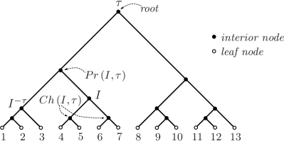
Figure 1: Hierarchical relations: parent - $Pr\left(I,\tau\right)$, children - $\mathrm{Ch}{\rm Phys.~{}Rev.~{}Lett.}{I,\tau}$, and local complement (sibling) - ${I}^{-\tau}$ of cluster $I$ of a rooted binary tree, $\tau\in\mathcal{BT}_{\left[13\right]}$. Filled and unfilled circles represent interior and leaf nodes, respectively. An interior node is referred by its cluster, the list of leaves below it; for example, $I=\left\{4,5,6,7\right\}$.

For every cluster $I\in\mathscr{C}\left(\tau\right)$ we recall the standard notion of parent (cluster) $Pr\left(I,\tau\right)$ and lists of children $\mathrm{Ch}{\rm Phys.~{}Rev.~{}Lett.}{I,\tau}$ of $I$ in $\tau$, illustrated in Figure 1. For the trivial case, we set $Pr\left(J,\tau\right)=\emptyset$. Additionally, we find it useful to define the local complement (sibling) of cluster $I\in\mathscr{C}\left(\tau\right)$ as ${I}^{-\tau}\>{\mathbf{:}=}\>Pr\left(I,\tau\right)\setminus I$, not to confused with the standard (global) complement ${I}^{C}=J\setminus I$. Further, a grandchild in $\tau$ is a cluster $G\in\mathscr{C}\left(\tau\right)$ having a grandparent $\mathrm{Pr}^{2}{\rm Phys.~{}Rev.~{}Lett.}{G,\tau}\>{\mathbf{:}=}\>$ $Pr\left(\big{.}Pr\left(G,\tau\right),\tau\right)$ in $\tau$. We denote the set of all grandchildren in $\tau$ by $\mathcal{G}{\rm Phys.~{}Rev.~{}Lett.}{\tau}$, the maximal subset of $\mathscr{C}\left(\tau\right)$ excluding the root $J$ and its children $\mathrm{Ch}{\rm Phys.~{}Rev.~{}Lett.}{J,\tau}$,

$$\mathcal{G}{\rm Phys.~{}Rev.~{}Lett.}{\tau} \>{\mathbf{:}=}\>\left\{G\in\mathscr{C}\left(\tau\right)\big{|}\mathrm{Pr}^{2}{\rm Phys.~{}Rev.~{}Lett.}{G,\tau}\neq\emptyset\right\},$$ (4a)

$$=\mathscr{C}\left(\tau\right)\setminus{\rm Phys.~{}Rev.~{}Lett.}{\big{.}\left\{J\right\}\cup\mathrm{Ch}{\rm Phys.~{}Rev.~{}Lett.}{J,\tau}}.$$ (4b)

A rooted tree with all interior vertices of out-degree two is said to be binary or, equivalently, non-degenerate, and all other trees are said to be degenerate. In this paper $\mathcal{BT}_{J}$ denotes the set of rooted nondegenerate trees over leaf set $J$. Note that the number of hierarchies in $\mathcal{BT}_{J}$ grows super exponentially [7],

$$\left|\mathcal{BT}_{J}\right|={\rm Phys.~{}Rev.~{}Lett.}{\big{.}2\left|J\right|-3}!!={\rm Phys.~{}Rev.~{}Lett.}{\big{.}2\left|J\right|-3}{\rm Phys.~{}Rev.~{}Lett.}{\big{.}2\left|J\right|-5}\ldots 3,$$ (5)

for $\left|J\right|\geq 2$, quickly precluding the possibility of exhaustive search for the “best" hierarchical clustering model in even modest problem settings.

2.3 Nearest Neighbor Interchange (NNI) Moves

Different notions of the neighborhood of a non-degenerate hierarchy in $\mathcal{BT}_{J}$ can be imposed by recourse to different tree restructuring operations [13] (or moves). NNI moves are particularly important for our setting because of their close relation with cluster hierarchy homogeneity (Definition 4) and their role in the anytime procedure introduced in Section 4.

A convenient restatement of the standard definition of NNI walks [33, 28] for rooted trees, illustrated in Figure 2, is:

Definition 1

The Nearest Neighbor Interchange (NNI) move at a grandchild $G\in\mathcal{G}{\rm Phys.~{}Rev.~{}Lett.}{\sigma}$ on a binary hierarchy $\sigma\in\mathcal{BT}_{J}$ swaps cluster $G$ with its parent’s sibling ${Pr\left(G,\sigma\right)}^{-\sigma}$ to yield another binary hierarchy $\tau\in\mathcal{BT}_{J}$.

We say that $\sigma,\tau\in\mathcal{BT}_{J}$ are NNI-adjacent if and only if one can be obtained from the other by a single NNI move.

More precisely, $\tau\in\mathcal{BT}_{J}$ is the result of performing the NNI move at grandchild $G\in\mathcal{G}{\rm Phys.~{}Rev.~{}Lett.}{\sigma}$ on $\sigma\in\mathcal{BT}_{J}$ if

$$\mathscr{C}\left(\tau\right) ={\rm Phys.~{}Rev.~{}Lett.}{\big{.}\mathscr{C}\left(\sigma\right)\setminus\left\{Pr\left(G,\sigma\right)\right\}}\cup\left\{\big{.}{I}^{-\sigma}\cup{G}^{-\sigma}\right\}.$$ (6)

Throughout the sequel we will denote the map of $\mathcal{BT}_{J}$ into itself defining an NNI move at a grandchild cluster of a tree $G\in\mathcal{G}{\rm Phys.~{}Rev.~{}Lett.}{\sigma}$ as $\tau=\text{NNI}{\rm Phys.~{}Rev.~{}Lett.}{\sigma,G}$.

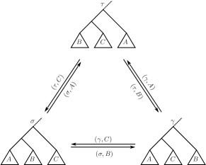
Figure 2: An illustration of NNI moves between binary trees: each arrow is labeled by a source tree and associated cluster defining the move.

A useful observation for NNI-adjacent hierarchies illustrating their structural difference is:

Lemma 1

[4] An ordered pair of hierarchies ${\rm Phys.~{}Rev.~{}Lett.}{\sigma,\tau}$ is NNI-adjacent if and only if there exists one and only one ordered triple ${\rm Phys.~{}Rev.~{}Lett.}{A,B,C}$ of common clusters of $\sigma$ and $\tau$ such that $\left\{A\cup B\right\}=\mathscr{C}\left(\sigma\right)\setminus\mathscr{C}\left(\tau\right)$ and $\left\{B\cup C\right\}=\mathscr{C}\left(\tau\right)\setminus\mathscr{C}\left(\sigma\right)$.

We call ${\rm Phys.~{}Rev.~{}Lett.}{A,B,C}$ the “NNI-triplet" of $\;{\rm Phys.~{}Rev.~{}Lett.}{\sigma,\tau}$.

2.4 Hierarchical Agglomerative Clustering

Given a choice of linkage, $\zeta:{\rm Phys.~{}Rev.~{}Lett.}{\mathbb{R}^{m}}^{J}\times\mathcal{P}{\rm Phys.~{}Rev.~{}Lett.}{J}\times\mathcal{P}{\rm Phys.~{}Rev.~{}Lett.}{J}\rightarrow\mathbb{R}_{\geq 0}$, Table 1 formalizes the associated Hierarchical Agglomerative $\zeta$-Clustering method [22]. This method yields a sequence of nested partitions of the dataset that can be represented by a tree with root at the coarsest, single cluster partition, leaves at the most refined trivial partition (comprising all singleton sets), and a vertex for each subset appearing in any of the successively coarsened partitions that appears as the mergers of Table 1 are imposed. Because only two clusters are merged at each step, the resulting sequence of nested partitions defines a binary tree, $\tau\in\mathcal{BT}_{J}$ whose nodes represent the clusters

$$\mathscr{C}\left(\tau\right)=\bigcup_{k=0}^{\left|J\right|-1}\mathcal{J}_{k}=\left\{J\right\}\cup\bigcup_{k=0}^{\left|J\right|-2}\left\{A^{*}_{k},B^{*}_{k}\right\}.$$ (7)

and whose edges represent the nesting relation, again as presented in Table 1. Hence, the set of grandchildren clusters $\mathcal{G}{\rm Phys.~{}Rev.~{}Lett.}{\tau}$ (4) of $\tau$ is given by

$$\mathcal{G}{\rm Phys.~{}Rev.~{}Lett.}{\tau}=\bigcup_{k=0}^{\left|J\right|-3}\mathcal{J}_{k}=\bigcup_{k=0}^{\left|J\right|-3}\left\{A^{*}_{k},B^{*}_{k}\right\}.$$ (8)

From this discussion it is clear that Table 1 defines a relation from datasets to trees, $\mathtt{HAC}_{\zeta}\subset{\rm Phys.~{}Rev.~{}Lett.}{\mathbb{R}^{m}}^{J}\times\mathcal{BT}_{J}$. Note that $\mathtt{HAC}_{\zeta}$ is in general not a function since there may well be more than one pair of clusters satisfying (9a) at any stage, $k$. It is, however, a multi-function: in other words, while agglomerative clustering of a dataset always yields some tree, that tree is not necessarily unique to that dataset.

Table 1: Hierarchical Agglomerative $\zeta$-Clustering​[22]

For any given set of data points $\mathrm{\mathbf{x}}\in{\rm Phys.~{}Rev.~{}Lett.}{\mathbb{R}^{m}}^{J}$ and linkage function  $\zeta:{\rm Phys.~{}Rev.~{}Lett.}{\mathbb{R}^{m}}^{J}\times\mathcal{P}{\rm Phys.~{}Rev.~{}Lett.}{J}\times\mathcal{P}{\rm Phys.~{}Rev.~{}Lett.}{J}\rightarrow\mathbb{R}_{\geq 0}$, • Begin with the finest partition of $J$, $\mathcal{J}_{0}=\left\{\big{.}\left\{i\right\}\right\}_{i\in J}$. • For every $k\in[0,\left|J\right|-1)$, merge two blocks of $\mathcal{J}_{k}$ with the minimum linkage value, $\displaystyle{\rm Phys.~{}Rev.~{}Lett.}{A^{*}_{k},B^{*}_{k}}=\operatornamewithlimits{arg\ min}_{A\neq B\in\mathcal{J}_{k}}\zeta{\rm Phys.~{}Rev.~{}Lett.}{\mathrm{\mathbf{x}};A,B},\hskip 34.1433pt$ (9a) $\displaystyle\mathcal{J}_{k+1}=\left\{A^{*}_{k}\cup B^{*}_{k}\right\}\cup\mathcal{J}_{k}\setminus\left\{A^{*}_{k},B^{*}_{k}\right\}.$ (9b)

2.4.1 Linkages

A linkage, $\zeta:{\rm Phys.~{}Rev.~{}Lett.}{\mathbb{R}^{m}}^{J}\times\mathcal{P}{\rm Phys.~{}Rev.~{}Lett.}{J}\times\mathcal{P}{\rm Phys.~{}Rev.~{}Lett.}{J}\rightarrow\mathbb{R}_{\geq 0}$, uses the dissimilarity of observations in the partial datasets, $\mathrm{\mathbf{x}}|A$ and $\mathrm{\mathbf{x}}|B$, to define dissimilarity between the clusters, $A,B\subseteq J$ and $\mathrm{\mathbf{x}}\in{\rm Phys.~{}Rev.~{}Lett.}{\mathbb{R}^{m}}^{\left|J\right|}$ [2]. Some common examples are

$$\zeta_{S}{\rm Phys.~{}Rev.~{}Lett.}{\mathrm{\mathbf{x}};A,B} \>{\mathbf{:}=}\>\min_{\begin{subarray}{c}a\in A\\ b\in B\end{subarray}}\mathit{d}{\rm Phys.~{}Rev.~{}Lett.}{\mathrm{x}_{a},\mathrm{x}_{b}},$$ (10a)

$$\zeta_{C}{\rm Phys.~{}Rev.~{}Lett.}{\mathrm{\mathbf{x}};A,B} \>{\mathbf{:}=}\>\max_{\begin{subarray}{c}a\in A\\ b\in B\end{subarray}}\mathit{d}{\rm Phys.~{}Rev.~{}Lett.}{\mathrm{x}_{a},\mathrm{x}_{b}},$$ (10b)

$$\zeta_{A}{\rm Phys.~{}Rev.~{}Lett.}{\mathrm{\mathbf{x}};A,B} \>{\mathbf{:}=}\>\frac{1}{\left|A\right|\left|B\right|}\sum_{\begin{subarray}{c}a\in A\\ b\in B\end{subarray}}\mathit{d}{\rm Phys.~{}Rev.~{}Lett.}{\mathrm{x}_{a},\mathrm{x}_{b}},$$ (10c)

$$\zeta_{M}{\rm Phys.~{}Rev.~{}Lett.}{\mathrm{\mathbf{x}};A,B} \>{\mathbf{:}=}\>\min_{a\in A\cup B}\max_{b\in A\cup B}\mathit{d}{\rm Phys.~{}Rev.~{}Lett.}{\mathrm{x}_{a},\mathrm{x}_{b}},$$ (10d)

$$\zeta_{W}{\rm Phys.~{}Rev.~{}Lett.}{\mathrm{\mathbf{x}};A,B} \>{\mathbf{:}=}\>\frac{\left|A\right|\left|B\right|}{\left|A\right|+\left|B\right|}\left\|\mathrm{c}{\rm Phys.~{}Rev.~{}Lett.}{\mathrm{\mathbf{x}}|A}-\mathrm{c}{\rm Phys.~{}Rev.~{}Lett.}{\mathrm{\mathbf{x}}|B}\right\|_{2}^{2}$$ (10e)

for single, complete, average, minimax and Ward’s linkages, respectively [22, 6], where $\mathit{d}$ and $\left\|.\right\|_{2}$ are a dissimilarity measure in $\mathbb{R}^{m}$ and the standard Euclidean norm , respectively.

A common way of characterizing linkages is through their behaviours after merging a set of clusters. For any pairwise disjoint subsets $A,B,C$ of $J$ and dataset $\mathrm{\mathbf{x}}\in{\rm Phys.~{}Rev.~{}Lett.}{\mathbb{R}^{m}}^{J}$, a linkage relation between partial observations $\mathrm{\mathbf{x}}|A\cup B$ and $\mathrm{\mathbf{x}}|C$ after merging $\mathrm{\mathbf{x}}|A$ and $\mathrm{\mathbf{x}}|B$ are generally described by the recurrence formula of Lance and Williams [25],

$$\zeta{\rm Phys.~{}Rev.~{}Lett.}{\mathrm{\mathbf{x}};\!A\!\cup\!B,\!C} =\alpha_{A}\zeta{\rm Phys.~{}Rev.~{}Lett.}{\mathrm{\mathbf{x}};\!A,\!C}+\alpha_{B}\zeta{\rm Phys.~{}Rev.~{}Lett.}{\mathrm{\mathbf{x}};\!B,\!C}+\beta\zeta{\rm Phys.~{}Rev.~{}Lett.}{\mathrm{\mathbf{x}};A,B}$$

$$\hskip 28.45274pt+\gamma\left|\big{.}\zeta{\rm Phys.~{}Rev.~{}Lett.}{\mathrm{\mathbf{x}};\!A,\!C}-\zeta{\rm Phys.~{}Rev.~{}Lett.}{\mathrm{\mathbf{x}};\!B,\!C}\right|,$$ (11)

where $\zeta:{\rm Phys.~{}Rev.~{}Lett.}{\mathbb{R}^{m}}^{J}\times\mathcal{P}{\rm Phys.~{}Rev.~{}Lett.}{J}\times\mathcal{P}{\rm Phys.~{}Rev.~{}Lett.}{J}\rightarrow\mathbb{R}_{\geq 0}$ is a linkage function and $\alpha_{A},\alpha_{B},\beta,\gamma\in\mathbb{R}$. Table 2 lists the coefficient of (11) for some common linkages in (10). Although the minimax linkage $\zeta_{M}$ (10d) can not be written in the form of the recurrence formula [6], as many other linkage functions above it satisfies

$$\zeta_{M}{\rm Phys.~{}Rev.~{}Lett.}{\mathrm{\mathbf{x}};A\cup B,C}\geq\min{\rm Phys.~{}Rev.~{}Lett.}{\big{.}\zeta_{M}{\rm Phys.~{}Rev.~{}Lett.}{\mathrm{\mathbf{x}};A,C},\zeta_{M}{\rm Phys.~{}Rev.~{}Lett.}{\mathrm{\mathbf{x}};B,C}},$$ (12)

which is known as the strong reducibility property, defined in the following paragraph.

Table 2: Coefficients of the recurrence formula of [25] for some common linkages

Linkage	$\alpha_{A}$	$\alpha_{B}$	$\beta$	$\gamma$
Single	$0.5$	$0.5$	$0$	$-0.5$
Complete	$0.5$	$0.5$	$0$	$0.5$
Average	$\Big{.}\frac{\left|A\right|}{\left|A\right|\!+\!\left|B\right|}$	$\frac{\left|B\right|}{\left|A\right|\!+\!\left|B\right|}$	$0$	$0$
Ward	$\Big{.}\frac{\left|A\right|\!+\!\left|C\right|}{\left|A\right|\!+\!\left|B\right|\!+\!\left|C\right|}$	$\frac{\left|B\right|\!+\!\left|C\right|}{\left|A\right|\!+\!\left|B\right|\!+\!\left|C\right|}$	$-\frac{\left|C\right|}{\left|A\right|\!+\!\left|B\right|\!+\!\left|C\right|}$	0

2.4.2 Reducibility & Monotonicity

Definition 2 ([10, 29])

For a fixed finite index set $J$, a linkage function $\zeta:{\rm Phys.~{}Rev.~{}Lett.}{\mathbb{R}^{m}}^{J}\times\mathcal{P}{\rm Phys.~{}Rev.~{}Lett.}{J}\times\mathcal{P}{\rm Phys.~{}Rev.~{}Lett.}{J}\rightarrow\mathbb{R}_{\geq 0}$ is said to be reducible if for any pairwise disjoint subsets $A,B,C$ of $J$ and set of data points $\mathrm{\mathbf{x}}\in{\rm Phys.~{}Rev.~{}Lett.}{\mathbb{R}^{m}}^{J}$

$$\zeta{\rm Phys.~{}Rev.~{}Lett.}{\mathrm{\mathbf{x}};A,B} \leq\min{\rm Phys.~{}Rev.~{}Lett.}{\big{.}\zeta{\rm Phys.~{}Rev.~{}Lett.}{\mathrm{\mathbf{x}};A,C},\zeta{\rm Phys.~{}Rev.~{}Lett.}{\mathrm{\mathbf{x}};B,C}}$$ (13a)

implies

$$\zeta{\rm Phys.~{}Rev.~{}Lett.}{\mathrm{\mathbf{x}};A\cup B,C}\geq\min{\rm Phys.~{}Rev.~{}Lett.}{\big{.}\zeta{\rm Phys.~{}Rev.~{}Lett.}{\mathrm{\mathbf{x}};A,C},\zeta{\rm Phys.~{}Rev.~{}Lett.}{\mathrm{\mathbf{x}};B,C}}.$$ (13b)

Further, say $\zeta$ is strongly reducible if for any pairwise disjoint subsets $A,B,C$ of $J$ and $\mathrm{\mathbf{x}}\in{\rm Phys.~{}Rev.~{}Lett.}{\mathbb{R}^{m}}^{J}$ it satisfies

$$\zeta{\rm Phys.~{}Rev.~{}Lett.}{\mathrm{\mathbf{x}};A\cup B,C}\geq\min{\rm Phys.~{}Rev.~{}Lett.}{\big{.}\zeta{\rm Phys.~{}Rev.~{}Lett.}{\mathrm{\mathbf{x}};A,C},\zeta{\rm Phys.~{}Rev.~{}Lett.}{\mathrm{\mathbf{x}};B,C}}.$$ (14)

The well known examples of linkages with the strong reducibility property are single, complete, average and minimax linkages in (10) [29, 6]. Even though Ward’s linkage is not strongly reducible, it still has the reducibility property.

A property of clustering hierarchies (of great importance in the sequel) consequent upon the reducibility property of linkages is monotonicity:

Definition 3 ([22])

A non-degenerate hierarchy $\tau\in\mathcal{BT}_{J}$ associated with a set of data points $\mathrm{\mathbf{x}}\in{\rm Phys.~{}Rev.~{}Lett.}{\mathbb{R}^{m}}^{J}$ is said to be $\zeta$-monotone if all grandchildren, $I\in\mathcal{G}{\rm Phys.~{}Rev.~{}Lett.}{\tau}$, are more similar to their siblings, ${I}^{-\tau}$, than are their parents, $P=Pr\left(I,\tau\right)$, i.e.

$$\zeta{\rm Phys.~{}Rev.~{}Lett.}{\mathrm{\mathbf{x}};I,{I}^{-\tau}}\leq\zeta{\rm Phys.~{}Rev.~{}Lett.}{\mathrm{\mathbf{x}};P,{P}^{-\tau}}.$$ (15)

Proposition 1 ([22])

If linkage $\zeta$ is reducible, then a cluster hierarchy $\tau\in\mathcal{BT}_{J}$ in the relation $\mathtt{HAC}_{\zeta}$ (i.e. resulting from procedure of Table 1 applied to some dataset $\mathrm{\mathbf{x}}\in{\rm Phys.~{}Rev.~{}Lett.}{\mathbb{R}^{m}}^{J}$) is always $\zeta$-monotone.

3 Homogeneity

We now introduce our new notion of homogeneity and explore its relationships to previously developed structural properties of trees.

Definition 4

(Homogeneity) A binary hierarchy $\tau\in\mathcal{BT}_{J}$ associated with a set of data points $\mathrm{\mathbf{x}}\in{\rm Phys.~{}Rev.~{}Lett.}{\mathbb{R}^{m}}^{J}$ is locally $\zeta$-homogeneous at grandchild cluster $I\in\mathcal{G}{\rm Phys.~{}Rev.~{}Lett.}{\tau}$ if the siblings, $I$ and ${I}^{-\tau}$, are closer to each other than to their parent’s sibling, ${P}^{-\tau}={Pr\left(I,\tau\right)}^{-\tau}$,

$$\zeta{\rm Phys.~{}Rev.~{}Lett.}{\mathrm{\mathbf{x}};I,{I}^{-\tau}}\leq\min{\rm Phys.~{}Rev.~{}Lett.}{\big{.}\zeta{\rm Phys.~{}Rev.~{}Lett.}{\mathrm{\mathbf{x}};I,{P}^{-\tau}},\zeta{\rm Phys.~{}Rev.~{}Lett.}{\mathrm{\mathbf{x}};{I}^{-\tau},{P}^{-\tau}}}.$$ (16)

A tree is $\zeta$-homogeneous if it is locally $\zeta$-homogeneous at each grandchild.

A useful observation when we focus attention on reducible linkages is:

Proposition 2

If a tree, $\tau\in\mathcal{BT}_{J}$ associated with a set of data points $\mathrm{\mathbf{x}}\in{\rm Phys.~{}Rev.~{}Lett.}{\mathbb{R}^{m}}^{J}$, is $\zeta$-homogeneous for a reducible linkage $\zeta$, then it must be $\zeta$-monotone as well.

Proof 3.1.

The result directly follows from homogeneity of $\tau$ and reducibility of $\zeta$.

For any grandchild cluster $I\in\mathcal{G}{\rm Phys.~{}Rev.~{}Lett.}{\tau}$ and its parent $P=Pr\left(I,\tau\right)$, using (13) and (16), one can verify the result as

$$\zeta{\rm Phys.~{}Rev.~{}Lett.}{\mathrm{\mathbf{x}};\!I,\!{I}^{-\tau}}\!\leq\!\min{\rm Phys.~{}Rev.~{}Lett.}{\big{.}\zeta{\rm Phys.~{}Rev.~{}Lett.}{\mathrm{\mathbf{x}};\!I,\!{P}^{-\tau}}\!,\zeta{\rm Phys.~{}Rev.~{}Lett.}{\mathrm{\mathbf{x}};\!{I}^{-\tau}\!\!,\!{P}^{-\tau}}\!}\!\leq\!\zeta{\rm Phys.~{}Rev.~{}Lett.}{\mathrm{\mathbf{x}};\!P,\!{P}^{-\tau}}\!\!,\!\!\!$$ (17)

where $P=I\cup{I}^{-\tau}$. ∎

The converse of Proposition 2 only holds for single linkage:

Proposition 3.2.

A clustering hierarchy $\tau\in\mathcal{BT}_{J}$ associated with a set of data points $\mathrm{\mathbf{x}}\in{\rm Phys.~{}Rev.~{}Lett.}{\mathbb{R}^{m}}^{J}$ is $\zeta_{S}$-monotone for single linkage $\zeta_{S}$ (10a) if and only if it is $\zeta_{S}$-homogeneous as well.

Proof 3.3.

The sufficiency of $\zeta_{S}$-homogeneity of a clustering tree for its $\zeta_{S}$-monotonicity directly follows from Proposition 2.

The other way of implication is evident from definitions of monotonicity (Definition 3) and single linkage $\zeta_{S}$ (10a), i.e. for any $I\in\mathcal{G}{\rm Phys.~{}Rev.~{}Lett.}{\tau}$ and $P=Pr\left(I,\tau\right)$,

$$\zeta_{S}{\rm Phys.~{}Rev.~{}Lett.}{\mathrm{\mathbf{x}};I,{I}^{-\tau}} \leq\zeta_{S}{\rm Phys.~{}Rev.~{}Lett.}{\mathrm{\mathbf{x}};P,{P}^{-\tau}},$$ (18)

$$=\min{\rm Phys.~{}Rev.~{}Lett.}{\big{.}\zeta_{S}{\rm Phys.~{}Rev.~{}Lett.}{\mathrm{\mathbf{x}};I,{P}^{-\tau}},\zeta_{S}{\rm Phys.~{}Rev.~{}Lett.}{\mathrm{\mathbf{x}};{I}^{-\tau},{P}^{-\tau}}},$$ (19)

where $P=I\cup{I}^{-\tau}$. ∎

A major significance of homogeneity is that it is a common characteristic feature of any clustering hierarchy resulting from agglomerative clustering using any strong reducible linkage:

Proposition 3.4.

If linkage $\zeta$ is strongly reducible then any non-degenerate hierarchy $\tau\in\mathcal{BT}_{J}$ in the relation $\mathtt{HAC}_{\zeta}$ (i.e. resulting from the procedure of Table 1 applied to some dataset $\mathrm{\mathbf{x}}\in{\rm Phys.~{}Rev.~{}Lett.}{\mathbb{R}^{m}}^{J}$ ) is $\zeta$-homogeneous.

Proof 3.5.

Let ${\rm Phys.~{}Rev.~{}Lett.}{\mathcal{J}_{k}}_{0\leq k\leq\left|J\right|-1}$ be a sequence of nested partitions of $J$, defining $\tau$ as in (7), resulting from agglomerative $\zeta$-clustering of $\mathrm{\mathbf{x}}$. Further, for $0\leq k\leq\left|J\right|-2\;$ let ${\rm Phys.~{}Rev.~{}Lett.}{A^{*}_{k},B^{*}_{k}}$ be a pair of clusters of $\mathcal{J}_{k}$ in (9a) with the minimum linkage value.

For $0\leq k\leq\left|J\right|-3$ and any (grandchild) cluster $C_{k}\in\mathcal{J}_{k}\setminus\left\{A^{*}_{k},B^{*}_{k}\right\}$, from (9a), we have

$$\zeta{\rm Phys.~{}Rev.~{}Lett.}{\mathrm{\mathbf{x}};A^{*}_{k},B^{*}_{k}}\leq\zeta{\rm Phys.~{}Rev.~{}Lett.}{\mathrm{\mathbf{x}};A_{k}^{*},C_{k}},$$ (20)

$$\zeta{\rm Phys.~{}Rev.~{}Lett.}{\mathrm{\mathbf{x}};A^{*}_{k},B^{*}_{k}}\leq\zeta{\rm Phys.~{}Rev.~{}Lett.}{\mathrm{\mathbf{x}};B_{k}^{*},C_{k}}.$$ (21)

Now, observe that the parent’s sibling ${{\rm Phys.~{}Rev.~{}Lett.}{A^{*}_{k}\cup B^{*}_{k}}}^{-\tau}$ of $A^{*}_{k}$ and $B^{*}_{k}$ can be written as the union of elements of a subset $\mathcal{D}$ of $\mathcal{J}_{k}\setminus{\rm Phys.~{}Rev.~{}Lett.}{A^{*}_{k},B^{*}_{k}}$,

$${{\rm Phys.~{}Rev.~{}Lett.}{A^{*}_{k}\cup B^{*}_{k}}}^{-\tau}=\bigcup_{D\in\mathcal{D}}D.$$ (22)

That is to say, the elements of $\mathcal{D}$ are merged in a way described by the sequence of nested partitions ${\rm Phys.~{}Rev.~{}Lett.}{\mathcal{J}_{k}}_{0\leq k\leq\left|J\right|-1}$ of $J$ such that their union finally yields ${{\rm Phys.~{}Rev.~{}Lett.}{A^{*}_{k}\cup B^{*}_{k}}}^{-\tau}$.

Hence, using strong reducibility of $\zeta$ and (20), one can verify that

$$\zeta{\rm Phys.~{}Rev.~{}Lett.}{\mathrm{\mathbf{x}};A^{*}_{k},{{\rm Phys.~{}Rev.~{}Lett.}{A^{*}_{k}\cup B^{*}_{k}}}^{-\tau}} =\zeta{\rm Phys.~{}Rev.~{}Lett.}{\mathrm{\mathbf{x}};A^{*}_{k},\bigcup_{D\in\mathcal{D}}D},$$ (23)

$$\geq\min_{D\in\mathcal{D}}\zeta{\rm Phys.~{}Rev.~{}Lett.}{\mathrm{\mathbf{x}};A^{*}_{k},D},$$ (24)

$$\geq\zeta{\rm Phys.~{}Rev.~{}Lett.}{\mathrm{\mathbf{x}};A^{*}_{k},B^{*}_{k}},$$ (25)

which, by symmetry, also holds for $B^{*}_{k}$,

$$\zeta{\rm Phys.~{}Rev.~{}Lett.}{\mathrm{\mathbf{x}};B^{*}_{k},{{\rm Phys.~{}Rev.~{}Lett.}{A^{*}_{k}\cup B^{*}_{k}}}^{-\tau}}\geq\zeta{\rm Phys.~{}Rev.~{}Lett.}{\mathrm{\mathbf{x}};A^{*}_{k},B^{*}_{k}}.$$ (26)

Thus, since $\mathcal{G}{\rm Phys.~{}Rev.~{}Lett.}{\tau}=\bigcup_{k=0}^{\left|J\right|-3}\left\{A^{*}_{k},B^{*}_{k}\right\}$ (8), the result follows. ∎

In particular, a critical observation for single linkage is:

Theorem 3.6.

A non-degenerate hierarchy $\tau\in\mathcal{BT}_{J}$ is in the relation $\mathtt{HAC}_{\zeta_{S}}$ (i.e. results from the procedure of Table 1 applied to some dataset $\mathrm{\mathbf{x}}\in{\rm Phys.~{}Rev.~{}Lett.}{\mathbb{R}^{m}}^{J}$ using $\zeta_{S}$ (10a) as the linkage) if and only if $\tau$ is $\zeta_{S}$-homogeneous (or, equivalently, $\zeta_{S}$-monotone).

Proof 3.7.

The sufficiency, of being a single linkage clustering hierarchy, for homogeneity is evident from Proposition 3.4.

To see the necessity of homogeneity, we will first prove that if $\tau$ is $\zeta_{S}$-homogeneous, then for any $I\in\mathcal{G}{\rm Phys.~{}Rev.~{}Lett.}{\tau}$ and nonempty subset $Q\subseteq J\setminus Pr\left(I,\tau\right)$ the following holds

$$\zeta_{S}{\rm Phys.~{}Rev.~{}Lett.}{\mathrm{\mathbf{x}};I,{I}^{-\tau}}\leq\zeta_{S}{\rm Phys.~{}Rev.~{}Lett.}{\mathrm{\mathbf{x}};I,Q}.$$ (27)

Observe that (27) states that the cost of merging any one of $I$ and ${I}^{-\tau}$ with another cluster $Q\subseteq J\setminus Pr\left(I,\tau\right)$ is greater and equal to the cost of merging $I$ and ${I}^{-\tau}$. Then, by induction, we conclude that $\tau$ is a possible outcome of agglomerative single linkage clustering of $\mathrm{\mathbf{x}}$.

Let $Anc\left(I,\tau\right)$ denote the set of ancestors of cluster $I\in\mathscr{C}\left(\tau\right)$ of $\tau$, except the root $J$,

$$Anc\left(I,\tau\right)\>{\mathbf{:}=}\>\left\{A\in\mathscr{C}\left(\tau\right)\setminus\left\{J\right\}\big{|}I\subsetneq A\right\}.$$ (28)

Using the definition of $\zeta_{S}$ (10a) and monotonicity of $\tau$, one can verify that for any grandchild $I\in\mathcal{G}{\rm Phys.~{}Rev.~{}Lett.}{\tau}$ and its ancestor $A\in Anc\left(I,\tau\right)$

$$\zeta_{S}{\rm Phys.~{}Rev.~{}Lett.}{\mathrm{\mathbf{x}};I,{I}^{-\tau}}\leq\zeta_{S}{\rm Phys.~{}Rev.~{}Lett.}{\mathrm{\mathbf{x}};A,{A}^{-\tau}}\leq\zeta_{S}{\rm Phys.~{}Rev.~{}Lett.}{\mathrm{\mathbf{x}};I,{A}^{-\tau}}.$$ (29)

Now observe that the global complement of $Pr\left(I,\tau\right)$ can be written as

$$J\setminus Pr\left(I,\tau\right)=\bigcup_{A\in Anc\left(I,\tau\right)}{A}^{-\tau}.$$ (30)

As a result, combining (29) and (30) yields

$$\zeta_{S}{\rm Phys.~{}Rev.~{}Lett.}{\mathrm{\mathbf{x}};I,J\setminus Pr\left(I,\tau\right)} =\zeta_{S}{\rm Phys.~{}Rev.~{}Lett.}{\mathrm{\mathbf{x}},I,\bigcup_{A\in Anc\left(I,\tau\right)}{A}^{-\tau}}$$ (31)

$$=\min_{A\in Anc\left(I,\tau\right)}\zeta_{S}{\rm Phys.~{}Rev.~{}Lett.}{\mathrm{\mathbf{x}};I;{A}^{-\tau}}$$ (32)

$$\geq\zeta_{S}{\rm Phys.~{}Rev.~{}Lett.}{\mathrm{\mathbf{x}};I,{I}^{-\tau}},$$ (33)

from which one can conclude (27) for single linkage $\zeta_{S}$.

Finally, using a proof by induction, the result of the theorem can be shown as follows:

• (Base Case) if $I,{I}^{-\tau}\in\mathscr{C}\left(\tau\right)$ are singleton clusters, then, since they satisfy (27), they can be merged at an appropriate step of the agglomerative clustering when the minimum cluster distance is equal to $\zeta_{S}{\rm Phys.~{}Rev.~{}Lett.}{\mathrm{\mathbf{x}};I,{I}^{-\tau}}$. Note that, due to (27), neither $I$ nor ${I}^{-\tau}$ can be merged with any other cluster $Q\subseteq J\setminus Pr\left(I,\tau\right)$ at a lower linkage value than $\zeta_{S}{\rm Phys.~{}Rev.~{}Lett.}{\mathrm{\mathbf{x}};I,{I}^{-\tau}}$.

• (Induction) Otherwise, suppose that $I$ and ${I}^{-\tau}$ are already constructed since their children also satisfy (27) and, by monotonicity, children $\left\{I_{L},I_{R}\right\}=\mathrm{Ch}{\rm Phys.~{}Rev.~{}Lett.}{I,\tau}$ of $I$ satisfies $\zeta_{S}{\rm Phys.~{}Rev.~{}Lett.}{\mathrm{\mathbf{x}};I_{L},I_{R}}\leq\zeta_{S}{\rm Phys.~{}Rev.~{}Lett.}{\mathrm{\mathbf{x}};I,{I}^{-\tau}}$ as do children of ${I}^{-\tau}$. Thus, since clusters $I$ and ${I}^{-\tau}$ satisfy (27), they can be directly aggregated when the merging cost, i.e. the value of minimum cluster distance in (9a), reaches $\zeta_{S}{\rm Phys.~{}Rev.~{}Lett.}{\mathrm{\mathbf{x}};I,{I}^{-\tau}}$.

∎

4 Anytime Hierarchical Clustering

Given a choice of linkage, $\zeta:{\rm Phys.~{}Rev.~{}Lett.}{\mathbb{R}^{m}}^{J}\times\mathcal{P}{\rm Phys.~{}Rev.~{}Lett.}{J}\times\mathcal{P}{\rm Phys.~{}Rev.~{}Lett.}{J}\rightarrow\mathbb{R}_{\geq 0}$, Table 3 presents the formal specification of our central contribution, the associated Anytime Hierarchical $\zeta$-Clustering method. Once again, this method defines a new relation from datasets to hierarchies, $\mathtt{AHC}_{\zeta}\subset{\rm Phys.~{}Rev.~{}Lett.}{\mathbb{R}^{m}}^{J}\times\mathcal{BT}_{J}$ that is generally not a function but rather a multi-function (i.e. all datasets yield some hierarchy, but not necessarily a unique one).

Table 3: Anytime Hierarchical $\zeta$-Clustering

For any given clustering hierarchy $\tau\in\mathcal{BT}_{J}$ associated with a set of data points $\mathrm{\mathbf{x}}\in{\rm Phys.~{}Rev.~{}Lett.}{\mathbb{R}^{m}}^{J}$, and linkage function $\zeta:{\rm Phys.~{}Rev.~{}Lett.}{\mathbb{R}^{m}}^{J}\times\mathcal{P}{\rm Phys.~{}Rev.~{}Lett.}{J}\times\mathcal{P}{\rm Phys.~{}Rev.~{}Lett.}{J}\rightarrow\mathbb{R}_{\geq 0}$, 1. If $\tau$ is $\zeta$-homogeneous, then terminate and return $\tau$. 2. Otherwise, (a) Find a grandchild cluster $I\in\mathcal{G}{\rm Phys.~{}Rev.~{}Lett.}{\tau}$ at which $\tau$ violates local homogeneity, i.e. $\displaystyle\zeta{\rm Phys.~{}Rev.~{}Lett.}{\mathrm{\mathbf{x}};I,{I}^{-\tau}}\!>\!\min{\rm Phys.~{}Rev.~{}Lett.}{\big{.}\zeta{\rm Phys.~{}Rev.~{}Lett.}{\mathrm{\mathbf{x}};\!I,\!{P}^{-\tau}}\!\!,\zeta{\rm Phys.~{}Rev.~{}Lett.}{\mathrm{\mathbf{x}};\!{I}^{-\tau}\!,\!{P}^{-\tau}}\!}\!,\!\!$ (34) where $P=Pr\left(I,\tau\right)$. (b) Then perform an NNI restructuring on $\tau$ at grandchild $G^{*}\in\mathrm{Ch}{\rm Phys.~{}Rev.~{}Lett.}{P,\tau}$ with the maximum dissimilarity to ${P}^{-\tau}$, i.e. swap $G^{*}$ with ${P}^{-\tau}$, $\displaystyle G^{*}=\operatornamewithlimits{arg\ max}_{G\in\mathrm{Ch}{\rm Phys.~{}Rev.~{}Lett.}{P,\tau}}\zeta{\rm Phys.~{}Rev.~{}Lett.}{\mathrm{\mathbf{x}};G,{P}^{-\tau}},$ (35a) $\displaystyle\tau\leftarrow\text{NNI}{\rm Phys.~{}Rev.~{}Lett.}{\tau,G^{*}},\hskip 42.67912pt$ (35b) and go to Step 1.

Because the procedure defining $\mathtt{AHC}_{\zeta}$ in Table 3 does not entail any obvious gradient-like greedy step as do many previously proposed iterative clustering methods, demonstrating that it terminates requires some analysis that we now present.

4.1 Proof of Convergence

For any non-degenerate hierarchy $\tau\in\mathcal{BT}_{J}$ associated with a set of data points $\mathrm{\mathbf{x}}\in{\rm Phys.~{}Rev.~{}Lett.}{\mathbb{R}^{m}}^{J}$ and a linkage function $\zeta$, we consider the sum of linkage values as an objective function to assess the quality of clustering,

$$H_{\mathrm{\mathbf{x}},\zeta}{\rm Phys.~{}Rev.~{}Lett.}{\tau}\>{\mathbf{:}=}\>\frac{1}{2}\sum_{I\in\mathscr{C}\left(\tau\right)}\zeta{\rm Phys.~{}Rev.~{}Lett.}{\mathrm{\mathbf{x}};I,{I}^{LC}}.$$ (36)

Intuitively, one might expect that hierarchical agglomerative clustering methods yield clustering hierarchies minimizing (36). However, they are generally known to be step-wise optimal greedy methods [16] with an exception that single linkage clustering always returns a globally optimal clustering tree in the sense of (36) due to its close relation with a minimum spanning tree of the data set [17]. In contrast, for example, as witness to the general sub-optimality of agglomerative clustering relative to (36), for Ward’s linkage $\zeta_{W}$ (10e) $H_{\mathrm{\mathbf{x}},\zeta_{W}}$ is constant and equal to the sum of squared error of $\mathrm{\mathbf{x}}$ (see Appendix A), i.e. for any $\tau\in\mathcal{BT}_{J}$

$$H_{\mathrm{\mathbf{x}},\zeta_{W}}{\rm Phys.~{}Rev.~{}Lett.}{\tau}=\sum_{i\in J}\left\|\mathrm{x}_{i}-\mathrm{c}{\rm Phys.~{}Rev.~{}Lett.}{\mathrm{\mathbf{x}}|J}\right\|_{2}^{2},$$ (37)

where $\mathrm{c}{\rm Phys.~{}Rev.~{}Lett.}{\mathrm{\mathbf{x}}|J}$ (1) denotes the centroid of $\mathrm{\mathbf{x}}|J$.

Let ${\rm Phys.~{}Rev.~{}Lett.}{\sigma,\tau}$ be a pair of NNI-adjacent (Definition 1) hierarchies in $\mathcal{BT}_{J}$ and ${\rm Phys.~{}Rev.~{}Lett.}{A,B,C}$ be the NNI-triplet (Lemma 1) of common clusters of $\sigma$ and $\tau$. Recall that $A\cup B\in\mathscr{C}\left(\sigma\right)\setminus\mathscr{C}\left(\tau\right)$ and $B\cup C\in\mathscr{C}\left(\tau\right)\setminus\mathscr{C}\left(\sigma\right)$ are only unshared clusters of $\sigma$ and $\tau$, respectively. Hence, one can write the change in the objective function $H_{\mathrm{\mathbf{x}},\zeta}$ (36) after the NNI transition from $\sigma$ to $\tau$ as

$$H_{\mathrm{\mathbf{x}},\zeta}{\rm Phys.~{}Rev.~{}Lett.}{\tau}\!-\!H_{\mathrm{\mathbf{x}},\zeta}{\rm Phys.~{}Rev.~{}Lett.}{\sigma} \!=\!\zeta{\rm Phys.~{}Rev.~{}Lett.}{\mathrm{\mathbf{x}};B,C}\!+\!\zeta{\rm Phys.~{}Rev.~{}Lett.}{\mathrm{\mathbf{x}};B\!\cup\!C,A}$$

$$\hskip 28.45274pt\!-\!\zeta{\rm Phys.~{}Rev.~{}Lett.}{\mathrm{\mathbf{x}};A,B}\!-\!\zeta{\rm Phys.~{}Rev.~{}Lett.}{\mathrm{\mathbf{x}};A\!\cup\!B,C}.$$ (38)

Here we find it useful to define a new class of linkages:

Definition 4.8.

A linkage $\zeta:{\rm Phys.~{}Rev.~{}Lett.}{\mathbb{R}^{m}}^{J}\times\mathcal{P}{\rm Phys.~{}Rev.~{}Lett.}{J}\times\mathcal{P}{\rm Phys.~{}Rev.~{}Lett.}{J}\rightarrow\mathbb{R}_{\geq 0}$ is NNI-reducible if for any set of data points $\mathrm{\mathbf{x}}\in{\rm Phys.~{}Rev.~{}Lett.}{\mathbb{R}^{m}}^{J}$ and pairwise disjoint subsets $A,B,C$ of $J$

$$\zeta{\rm Phys.~{}Rev.~{}Lett.}{\mathrm{\mathbf{x}};B,C}\leq\min{\rm Phys.~{}Rev.~{}Lett.}{\big{.}\zeta{\rm Phys.~{}Rev.~{}Lett.}{\mathrm{\mathbf{x}};A,B},\zeta{\rm Phys.~{}Rev.~{}Lett.}{\mathrm{\mathbf{x}};A,C}}.$$ (39a)

implies

$$\min{\rm Phys.~{}Rev.~{}Lett.}{\!\!\!\!\begin{array}[]{l}\zeta{\rm Phys.~{}Rev.~{}Lett.}{\mathrm{\mathbf{x}};\!A,\!B}\!+\!\zeta{\rm Phys.~{}Rev.~{}Lett.}{\mathrm{\mathbf{x}};\!A\!\cup\!B,\!C}\!,\\ \zeta{\rm Phys.~{}Rev.~{}Lett.}{\mathrm{\mathbf{x}};\!A,\!C}\!+\!\zeta{\rm Phys.~{}Rev.~{}Lett.}{\mathrm{\mathbf{x}};\!A\!\cup\!C,\!B}\end{array}\!\!\!\!\!}\!\geq\!\zeta{\rm Phys.~{}Rev.~{}Lett.}{\mathrm{\mathbf{x}};\!B,\!C}\!+\!\zeta{\rm Phys.~{}Rev.~{}Lett.}{\mathrm{\mathbf{x}};\!B\!\cup\!C,\!A}\!.\!\!\!$$ (39d)

Using (10), (11) and Table 2 one can verify that single, complete, minimax and Ward’s linkages are examples of NNI-reducible linkages. Note that a reducible linkage is not necessarily NNI-reducible; for instance, average linkage $\zeta_{A}$ (10c).

We now proceed to investigate the termination of anytime hierarchical clustering for NNI-reducible linkages:

Lemma 4.9.

For any set of data points $\mathrm{\mathbf{x}}\in{\rm Phys.~{}Rev.~{}Lett.}{\mathbb{R}^{m}}^{J}$ and NNI-reducible linkage $\zeta$, the value of objective function $H_{\mathrm{\mathbf{x}},\zeta}$ (36) is nonincreasing at each iteration of anytime hierarchical clustering in Table 3 from any initial hierarchy $\sigma\in\mathcal{BT}_{J}$ towards $\tau\in\mathcal{BT}_{J}$,

$$H_{\mathrm{\mathbf{x}},\zeta}{\rm Phys.~{}Rev.~{}Lett.}{\tau}-H_{\mathrm{\mathbf{x}},\zeta}{\rm Phys.~{}Rev.~{}Lett.}{\sigma}\leq 0.$$ (40)

Proof 4.10.

If $\sigma$ is $\zeta$-homogeneous, then $\tau=\sigma$, and so the result directly follows.

Otherwise, let ${\rm Phys.~{}Rev.~{}Lett.}{A,B,C}$ be the NNI-triplet (Lemma 1) associated with ${\rm Phys.~{}Rev.~{}Lett.}{\sigma,\tau}$. Recall that $A\cup B\in\mathscr{C}\left(\sigma\right)\setminus\mathscr{C}\left(\tau\right)$ and $B\cup C\in\mathscr{C}\left(\tau\right)\setminus\mathscr{C}\left(\sigma\right)$. To put it another way, anytime hierarchical clustering performs an NNI move on $\sigma$ at grandchild $A\in\mathcal{G}{\rm Phys.~{}Rev.~{}Lett.}{\tau}$ towards $\tau$, and so

$$\zeta{\rm Phys.~{}Rev.~{}Lett.}{\mathrm{\mathbf{x}};A,B} >\zeta{\rm Phys.~{}Rev.~{}Lett.}{\mathrm{\mathbf{x}};B,C},$$ (41)

$$\zeta{\rm Phys.~{}Rev.~{}Lett.}{\mathrm{\mathbf{x}};A,C} \geq\zeta{\rm Phys.~{}Rev.~{}Lett.}{\mathrm{\mathbf{x}};B,C}.$$ (42)

Therefore, since $\zeta$ is NNI-reducible (Definition 4.8), the change in the objective function $H_{\mathrm{\mathbf{x}},\zeta}$ (4.1) is nonnegative,

$$H_{\mathrm{\mathbf{x}},\zeta}{\rm Phys.~{}Rev.~{}Lett.}{\tau}-H_{\mathrm{\mathbf{x}},\zeta}{\rm Phys.~{}Rev.~{}Lett.}{\sigma} \leq 0,$$ (43)

which completes the proof. ∎

Theorem 4.11.

If $\zeta$ is an NNI-reducible linkage, then iterated application of the Anytime Hierarchical $\zeta$-Clustering procedure of Table 3 initiated from any hierarchy in $\mathcal{BT}_{J}$ for a fixed set of data points $\mathrm{\mathbf{x}}\in{\rm Phys.~{}Rev.~{}Lett.}{\mathbb{R}^{m}}^{J}$ must terminate in finite time at a tree in $\mathcal{BT}_{J}$, that is $\zeta$-homogeneous.

Proof 4.12.

For a fixed finite index set $J$, the number of non-degenerate hierarchies in $\mathcal{BT}_{J}$ (5) is finite. Hence, for the proof of theorem, we shall show that the anytime clustering procedure in Table 3 can not yield any cycle in $\mathcal{BT}_{J}$.

Let $\tau^{k}\in\mathcal{BT}_{J}$ denote a clustering hierarchy visited at $k$-th iteration of anytime clustering method, where $k\geq 0$. Since $\tau^{k}$ and $\tau^{k+1}$ are NNI-adjacent, let ${\rm Phys.~{}Rev.~{}Lett.}{A^{k},B^{k},C^{k}}$ be the associated NNI-triplet (Lemma 1) of the pair ${\rm Phys.~{}Rev.~{}Lett.}{\tau^{k},\tau^{k+1}}$ satisfying $A^{k}\cup B^{k}\in\mathscr{C}\left(\tau^{k}\right)\setminus\mathscr{C}\left(\tau^{k+1}\right)$ and $B^{k}\cup C^{k}\in\mathscr{C}\left(\tau^{k+1}\right)\setminus\mathscr{C}\left(\tau^{k}\right)$. Further, recall from Lemma 4.9 that for any NNI-reducible linkage $\zeta$, $H_{\mathrm{\mathbf{x}};\zeta}{\rm Phys.~{}Rev.~{}Lett.}{\tau^{k+1}}-H_{\mathrm{\mathbf{x}};\zeta}{\rm Phys.~{}Rev.~{}Lett.}{\tau^{k}}\leq 0$.

If $H_{\mathrm{\mathbf{x}};\zeta}{\rm Phys.~{}Rev.~{}Lett.}{\tau^{k+1}}-H_{\mathrm{\mathbf{x}};\zeta}{\rm Phys.~{}Rev.~{}Lett.}{\tau^{k}}<0$, it is clear that anytime clustering method never revisits any previously visited clustering hierarchy.

Otherwise, $H_{\mathrm{\mathbf{x}};\zeta}{\rm Phys.~{}Rev.~{}Lett.}{\tau^{k+1}}=H_{\mathrm{\mathbf{x}};\zeta}{\rm Phys.~{}Rev.~{}Lett.}{\tau^{k}}$, we have

$$\zeta\!{\rm Phys.~{}Rev.~{}Lett.}{\!\mathrm{\mathbf{x}};\!A^{k}\!,\!B^{k}\!}\!+\!\zeta\!{\rm Phys.~{}Rev.~{}Lett.}{\!\mathrm{\mathbf{x}};\!A^{k}\!\cup\!B^{k}\!,\!C^{k}\!} \!=\!\zeta\!{\rm Phys.~{}Rev.~{}Lett.}{\!\mathrm{\mathbf{x}};\!B^{k}\!,\!C^{k}\!}\!+\!\zeta\!{\rm Phys.~{}Rev.~{}Lett.}{\!\mathrm{\mathbf{x}};\!B^{k}\!\cup\!C^{k}\!,\!A^{k}\!}\!\!,\!\!\!\!$$ (44)

$$\zeta{\rm Phys.~{}Rev.~{}Lett.}{\mathrm{\mathbf{x}};\!A^{k}\!,\!B^{k}} \!>\!\zeta{\rm Phys.~{}Rev.~{}Lett.}{\mathrm{\mathbf{x}};\!B^{k},\!C^{k}},$$ (45)

where the later is due to the anytime clustering rule in Table 3. Hence, the construction cost of (grand)parent $P^{k}=A^{k}\cup B^{k}\cup C^{k}$ increases after the NNI move,

$$\zeta{\rm Phys.~{}Rev.~{}Lett.}{\mathrm{\mathbf{x}};A^{k}\cup B^{k},C^{k}}<\zeta{\rm Phys.~{}Rev.~{}Lett.}{\mathrm{\mathbf{x}};B^{k}\cup C^{k},A^{k}}.$$ (46)

Now, let $0pt{\tau}{\rm Phys.~{}Rev.~{}Lett.}{I}$ denote the level of cluster $I\in\mathscr{C}\left(\tau\right)$ of $\tau\in\mathcal{BT}_{J}$ which is equal to the number of ancestors of $I$ in $\tau$,

$$0pt{\tau}{\rm Phys.~{}Rev.~{}Lett.}{I}\>{\mathbf{:}=}\>\left|\left\{A\in\mathscr{C}\left(\tau\right)\big{|}I\subseteq A\right\}\right|,$$ (47)

and define $L{\rm Phys.~{}Rev.~{}Lett.}{\tau}$ to be an ordered ${\rm Phys.~{}Rev.~{}Lett.}{\left|J\right|-1}$-tuple of sum of linkages of $\tau$ at each level,

$$L{\rm Phys.~{}Rev.~{}Lett.}{\tau} \>{\mathbf{:}=}\>{\rm Phys.~{}Rev.~{}Lett.}{\big{.}f_{\tau}{\rm Phys.~{}Rev.~{}Lett.}{t}}_{1\leq t\leq\left|J\right|-1},$$

$$={\rm Phys.~{}Rev.~{}Lett.}{\big{.}f_{\tau}{\rm Phys.~{}Rev.~{}Lett.}{1},f_{\tau}{\rm Phys.~{}Rev.~{}Lett.}{2},\ldots,f_{\tau}{\rm Phys.~{}Rev.~{}Lett.}{\left|J\right|-1}},$$ (48)

where a binary hierarchy over leaf set $J$ might have at most $\left|J\right|-1$ levels, and

$$f_{\tau}{\rm Phys.~{}Rev.~{}Lett.}{t}\>{\mathbf{:}=}\>\frac{1}{2}\sum_{\begin{subarray}{c}I\in\mathscr{C}\left(\tau\right)\\ 0pt{\tau}{\rm Phys.~{}Rev.~{}Lett.}{I}=t\end{subarray}}\zeta{\rm Phys.~{}Rev.~{}Lett.}{\mathrm{\mathbf{x}};I,{I}^{-\tau}}.$$ (49)

Note that if there is no cluster at level $t$ of $\tau$, then we set $f_{\tau}{\rm Phys.~{}Rev.~{}Lett.}{t}=0$.

Have $(\left|J\right|-1)$-tuples of real numbers ordered lexicographically according to the standard order of reals. Then, since NNI transition from $\tau^{k}$ to $\tau^{k+1}$ might only change linkages between clusters below (grand)parent cluster $P^{k}=A^{k}\cup B^{k}\cup C^{k}$, using (46), one can conclude that

$$L{\rm Phys.~{}Rev.~{}Lett.}{\tau^{k}}<L{\rm Phys.~{}Rev.~{}Lett.}{\tau^{k+1}}.$$ (50)

Thus, it is also impossible to visit the same clustering hierarchy at the same level of objective function $H_{\mathrm{\mathbf{x}},\zeta}$, which completes the proof. ∎

Even though average linkage $\zeta_{A}$ (10c) is not NNI-reducible, as shown in Appendix B, anytime hierarchical clustering based on average linkage still has the finite time termination property.

4.2 A Brief Discussion of Computational
Properties

Complexity analysis of any recursive algorithm will necessarily engage two logically independent questions: (i) how many iterations are required to convergence; and (ii) what computational cost is incurred by application of the recursive function at each step along the way? Accordingly, in this section we address this pair of question in the context of the anytime hierarchical clustering algorithm of Table 3. Specifically we : (i) discuss (but defer to a subsequent paper a complete treatment of) the problem of determining bounds on the number of iterations of anytime clustering; and (ii) present explicit bounds on the computational cost of checking whether a cluster hierarchy violates local homogeneity at a given cluster (node) of tree or not. Prior work on discriminative comparison of non-degenerate hierarchies [4] and the results of experimental evaluation in Section 5 hint at a bound on the number of iterations (i) that is $\mathrm{O}{\rm Phys.~{}Rev.~{}Lett.}{n^{2}}$ with the dataset cardinality, $n$. We leave a comprehensive detailed study of algorithmic complexity of anytime hierarchical clustering to a future discussion of specific implementations. However, we still find it useful to give a brief idea of the computational cost incurred by the determination of tree homogeneity with respect to a number of commonly used linkages.

A straightforward implementation to check (ii) local homogeneity of a clustering hierarchy at any cluster with respect to any linkage function in (10) generally has time complexity of $\mathrm{O}{\rm Phys.~{}Rev.~{}Lett.}{n^{2}}$ with the dataset size, $n$, with an exception that local homogeneity of a clustering tree relative to Ward’s linkage can be computed in linear, $\mathrm{O}{\rm Phys.~{}Rev.~{}Lett.}{n}$, time.

Alternatively, following the CF(Clustering Feature) tree of BIRCH [41], a simple tree data structure can be used to store sufficient statistics, such as cluster sizes, means and variances, of a clustering hierarchy associated with a dataset. Such a data structure can be constructed in linear time, with the dataset size, using a post-order traversal of a clustering tree and the following recursion of cluster sizes, means and variances. For any $\mathrm{\mathbf{x}}\in{\rm Phys.~{}Rev.~{}Lett.}{\mathbb{R}^{m}}^{J}$ and disjoint subsets $A,B\subseteq J$ of a finite index set $J$, the sufficient statistics of $\mathrm{\mathbf{x}}|A\cup B$ can be written in terms of the sufficient statistics of $\mathrm{\mathbf{x}}|A$ and $\mathrm{\mathbf{x}}|B$ as follows:

$$\left|A\cup B\right| \!=\!\left|A\right|+\left|B\right|,$$ (51a)

$$\mathrm{c}{\rm Phys.~{}Rev.~{}Lett.}{\mathrm{\mathbf{x}}|A\!\cup\!B} \!=\!{$\frac{\left|A\right|}{\left|A\right|+\left|B\right|}$}\mathrm{c}{\rm Phys.~{}Rev.~{}Lett.}{\mathrm{\mathbf{x}}|A}\!+\!{$\frac{\left|B\right|}{\left|A\right|+\left|B\right|}$}\mathrm{c}{\rm Phys.~{}Rev.~{}Lett.}{\mathrm{\mathbf{x}}|B}\!,$$ (51b)

$$\mathrm{v}{\rm Phys.~{}Rev.~{}Lett.}{\mathrm{\mathbf{x}}|A\!\cup\!B} \!=\!{$\frac{\left|A\right|}{\left|A\right|\!+\!\left|B\right|}$}\mathrm{v}{\rm Phys.~{}Rev.~{}Lett.}{\mathrm{\mathbf{x}}|A}\!+\!{$\frac{\left|B\right|}{\left|A\right|\!+\!\left|B\right|}$}\mathrm{v}{\rm Phys.~{}Rev.~{}Lett.}{\mathrm{\mathbf{x}}|B}$$

$$\hskip 45.5244pt\!+\!{$\frac{\left|A\right|\left|B\right|}{{\rm Phys.~{}Rev.~{}Lett.}{\left|A\right|\!+\!\left|B\right|}^{2}}$}\!\left\|\big{.}\mathrm{c}{\rm Phys.~{}Rev.~{}Lett.}{\mathrm{\mathbf{x}}|A}\!-\!\mathrm{c}{\rm Phys.~{}Rev.~{}Lett.}{\mathrm{\mathbf{x}}|B}\right\|_{2}^{2},$$ (51c)

where for any $I\subseteq J\;$ $\mathrm{c}{\rm Phys.~{}Rev.~{}Lett.}{\mathrm{\mathbf{x}}|I}$(1) and $\mathrm{v}{\rm Phys.~{}Rev.~{}Lett.}{\mathrm{\mathbf{x}}|I}$(2) denote the centroid and variance of $\mathrm{\mathbf{x}}|I$, respectively. Note that any singleton cluster $i\in\mathscr{C}\left(\tau\right)$ has $\left|i\right|=1$, $\mathrm{c}{\rm Phys.~{}Rev.~{}Lett.}{\mathrm{\mathbf{x}}|i}=\mathrm{x}_{i}$ and $\mathrm{v}{\rm Phys.~{}Rev.~{}Lett.}{\mathrm{\mathbf{x}}|i}=0$. Also, note that after an NNI restructuring of a clustering tree, the data structure keeping cluster sizes, means and variances can be updated in constant time using (51). Therefore, given the sufficient statistics, local homogeneity of a clustering hierarchy at any cluster with respect to Ward’s linkage can be determined in constant time.

To demonstrate another computationally efficient setting of anytime hierarchical clustering, consider the squared Euclidean distance as a dissimilarity measure, i.e. for any $\mathrm{x},\mathrm{y}\in\mathbb{R}^{m}$

$$\mathit{d}{\rm Phys.~{}Rev.~{}Lett.}{\mathrm{x},\mathrm{y}}=\left\|\mathrm{x}-\mathrm{y}\right\|_{2}^{2}.$$ (52)

As shown in Appendix C, for any $\mathrm{\mathbf{x}}\in{\rm Phys.~{}Rev.~{}Lett.}{\mathbb{R}^{m}}^{J}$ and disjoint subsets $A,B\subseteq J$, the average linkage $\zeta_{A}$ (10c) between partial patterns $\mathrm{\mathbf{x}}|A$ and $\mathrm{\mathbf{x}}|B$, based on the squared Euclidean distance, can be rewritten in terms of sufficient statistics of $\mathrm{\mathbf{x}}|A$ and $\mathrm{\mathbf{x}}|B$ as

$$\zeta_{A}\!{\rm Phys.~{}Rev.~{}Lett.}{\mathrm{\mathbf{x}};\!A,\!B}\!=\!\mathrm{v}{\rm Phys.~{}Rev.~{}Lett.}{\mathrm{\mathbf{x}}|A}+\mathrm{v}{\rm Phys.~{}Rev.~{}Lett.}{\mathrm{\mathbf{x}}|B}+\left\|\mathrm{c}{\rm Phys.~{}Rev.~{}Lett.}{\mathrm{\mathbf{x}}|A}-\mathrm{c}{\rm Phys.~{}Rev.~{}Lett.}{\mathrm{\mathbf{x}}|B}\right\|_{2}^{2}.$$ (53)

Therefore, as in the case of Ward’s linkage, given the sufficient statistics of a clustering hierarchy its local homogeneity at any cluster with respect to average linkage with the squared Euclidean distance (52) can be determined in constant time.

Table 4: Determining Local Homogeneity of a Clustering Hierarchy at any Cluster

Linkage	Single	Complete	Average	Ward	Minimax	Average
						with
						(52) or (54)
Complexity.	$\mathrm{O}{\rm Phys.~{}Rev.~{}Lett.}{n^{2}}$	$\mathrm{O}{\rm Phys.~{}Rev.~{}Lett.}{n^{2}}$	$\mathrm{O}{\rm Phys.~{}Rev.~{}Lett.}{n^{2}}$	$\mathrm{O}{\rm Phys.~{}Rev.~{}Lett.}{1}$	$\mathrm{O}{\rm Phys.~{}Rev.~{}Lett.}{n^{2}}$	$\mathrm{O}{\rm Phys.~{}Rev.~{}Lett.}{1}$

$n$: the number of data points

A similar computational improvement for average linkage is also possible with the cosine dissimilarity — another commonly used dissimilarity, in information retrieval and text mining [34]: for any $\mathrm{x},\mathrm{y}\in\mathbb{R}^{m}$,

$$\mathit{d}{\rm Phys.~{}Rev.~{}Lett.}{\mathrm{x},\mathrm{y}}=1-\frac{\mathrm{x}\cdot\mathrm{y}}{\left\|\mathrm{x}\right\|_{2}\left\|\mathrm{y}\right\|_{2}},$$ (54)

where $\cdot$ denote the Euclidean dot product. For any dataset of unit length vectors $\mathrm{\mathbf{x}}\in{\rm Phys.~{}Rev.~{}Lett.}{\mathbb{S}^{m-1}}^{J}$ and disjoint subsets $A,B\subseteq J$, the average linkage $\zeta_{A}$ (10c) between $\mathrm{\mathbf{x}}|A$ and $\mathrm{\mathbf{x}}|B$, based on the cosine dissimilarity, is given by

$$\zeta_{A}{\rm Phys.~{}Rev.~{}Lett.}{\mathrm{\mathbf{x}};A,B}=1-\mathrm{c}{\rm Phys.~{}Rev.~{}Lett.}{\mathrm{\mathbf{x}}|A}\cdot\mathrm{c}{\rm Phys.~{}Rev.~{}Lett.}{\mathrm{\mathbf{x}}|B}.$$ (55)

Table 4 briefly summaries the discussion on computational complexity of the determination of local homogeneity of a clustering hierarchy at any cluster.

4.3 Application: Incremental Clustering

As an application of anytime clustering, given a choice of linkage $\zeta$, we now propose an incremental hierarchical clustering method consisting of the following steps: (i) insert a new data point to existing clustering hierarchy based on a specific tree traversal and local homogeneity criterion as described in Table 5, and then (ii) apply anytime clustering of Table 3 to obtain a homogeneous clustering hierarchy of the updated data set with respect to $\zeta$.

Table 5: Incremental Hierarchical $\zeta$-Clustering: Data Insertion Using Local Homogeneity

Let $\tau\in\mathcal{BT}_{J}$ be a clustering hierarchy associated with a set of data points $\mathrm{\mathbf{x}}\in{\rm Phys.~{}Rev.~{}Lett.}{\mathbb{R}^{m}}^{J}$ and $\zeta$ be a linkage function. Let $i\not\in J$ denote the label of a new data point $\mathrm{x}_{i}\in\mathbb{R}^{m}$ to be inserted, and $\hat{J}=J\cup\left\{i\right\}$ and $\hat{\mathrm{\mathbf{x}}}={\rm Phys.~{}Rev.~{}Lett.}{\mathrm{x}_{j}}_{j\in\hat{J}}$ be the updated index and data sets after data insertion, respectively. To insert $\mathrm{x}_{i}$ into the existing clustering hierarchy $\tau$ associated with $\mathrm{\mathbf{x}}$: 1. Start with $K=J$. 2. For $\left\{K_{L},K_{R}\right\}=\mathrm{Ch}{\rm Phys.~{}Rev.~{}Lett.}{K,\tau}$, (a) If $\zeta{\rm Phys.~{}Rev.~{}Lett.}{\hat{\mathrm{\mathbf{x}}};\!K_{L},\!K_{R}}\!\leq\!\min{\rm Phys.~{}Rev.~{}Lett.}{\big{.}\zeta{\rm Phys.~{}Rev.~{}Lett.}{\hat{\mathrm{\mathbf{x}}};\!K_{L},\!\left\{i\right\}}\!,\zeta{\rm Phys.~{}Rev.~{}Lett.}{\hat{\mathrm{\mathbf{x}}};\!K_{R},\!\left\{i\right\}}}$, then   attach leaf $i$ as the sibling of $K$ in the new clustering tree $\hat{\tau}\in\mathcal{BT}_{\hat{J}}$. (b) Otherwise, set $K\!=\!\operatornamewithlimits{arg\ min}_{D\in\mathrm{Ch}{\rm Phys.~{}Rev.~{}Lett.}{K,\tau}}\zeta{\rm Phys.~{}Rev.~{}Lett.}{\hat{\mathrm{\mathbf{x}}};\!D\!,\left\{i\right\}\!}$, and go to step 2.

Note that, given the linkage values of a clustering hierarchy, for any linkage function satisfying the recurrence formula (11) of Lance and Williams [25] a data insertion, described in Table 5, can be performed in linear, $\mathrm{O}{\rm Phys.~{}Rev.~{}Lett.}{n}$, time with the dataset size, $n$. This follows because the linkage distance between the new data point and clusters of an existing hierarchy can be efficiently computed in linear time using a post-order traversal of the clustering hierarchy and (11).

5 Experimental Evaluation

This section presents a preliminary comparative numerical study of three different hierarchical clustering methods using both simulated and real datasets. We compare: (a) the standard agglomerative batch method ($\mathtt{HAC}_{\zeta}$, Table 1); with (b) the new anytime method ($\mathtt{AHC}_{\zeta}$, Table 3) and (c) its specialization to the incremental “data insertion" problem setting ($\mathtt{IHC}_{\zeta}$,Table 5).

5.1 Datasets

Very high dimensional and sparse data sets generally have simple structure and, specifically, are known to tend toward ultrametricity with the increasing dimensionality and/or sparsity[30]. In this context, the fact that a monotone clustering hierarchy associated with a dataset defines an ultrametric between data points (as we will briefly review in the next section) [11], motivates the intuition that hierarchical methods may enjoy particular efficacy in clustering problems involving high dimensional and sparse data. In the following preliminary study we will compare the results of hierarchical clustering on a low dimensional synthetic dataset and a higher dimensional dataset of physical origin. In both cases we will use a validation measure (introduced below) that quantifies the loss of information incurred by approximating the underlying pairwise dissimilarities between points with the coarsened measure arising from the ultrametric induced by the resulting cluster hierarchy.

A challenging dataset for any hierarchical clustering method consists of uniformly distributed low dimensional data points. We generate our synthetic data by uniformly sampling the planar unit cell, $\left[0,1\right]\times\left[0,1\right]$, thereby generating similar populations of varied cardinality. In contrast, for real data points, we use the MNIST collection of handwritten digits, where each data sample is a black and white $28\times 28$ image of a human produced numeral [26]. We generate test datasets of varied size by randomly sampling an equal number of images for each digit in the MNIST dataset.

5.2 Validation Measure

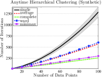
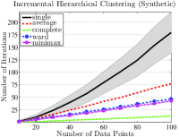
Figure 3: Average number of iterations of anytime (left) and incremental (right) hierarchical clusterings of simulated data points. Shaded regions illustrate the sample variance for the single linkage.

To evaluate the accuracy and effectiveness of different hierarchical clustering methods, we use the cophenetic correlation coefficient — a widely accepted validation criterion that measures how well a clustering hierarchy preserves the underlying pairwise dissimilarities between points in a dataset[37]. In order to interpret this criterion we find it helpful to briefly review the manner in which a monotone hierarchy induces an ultrametric between points in a dataset [11].

For any set of data points $\mathrm{\mathbf{x}}\in{\rm Phys.~{}Rev.~{}Lett.}{\mathbb{R}^{m}}^{J}$ and a clustering hierarchy $\tau\in\mathcal{BT}_{J}$ associated with $\mathrm{\mathbf{x}}$ and a linkage $\zeta$, let $\mathrm{\mathbf{D}}{\rm Phys.~{}Rev.~{}Lett.}{\mathrm{\mathbf{x}}}\in\mathbb{R}^{J}\times\mathbb{R}^{J}$ and $\mathrm{\mathbf{U}}_{\tau}{\rm Phys.~{}Rev.~{}Lett.}{\mathrm{\mathbf{x}}}\in\mathbb{R}^{J}\times\mathbb{R}^{J}$ denote the original distance matrix of $\mathrm{\mathbf{x}}$ and induced ultrametric of $\tau$, respectively. Namely, for any $I\in\mathscr{C}\left(\tau\right)$, $i\in I$ and $j\in{I}^{-\tau}$

$$\mathrm{\mathbf{D}}{\rm Phys.~{}Rev.~{}Lett.}{\mathrm{\mathbf{x}}}_{ij} =\left\|\mathrm{x}_{i}-\mathrm{x}_{j}\right\|_{2},$$ (56)

$$\mathrm{\mathbf{U}}_{\tau}{\rm Phys.~{}Rev.~{}Lett.}{\mathrm{\mathbf{x}}}_{ij} =\zeta{\rm Phys.~{}Rev.~{}Lett.}{\mathrm{\mathbf{x}};I,{I}^{-\tau}},$$ (57)

and for any $i\in J$ set $\mathrm{\mathbf{D}}{\rm Phys.~{}Rev.~{}Lett.}{\mathrm{\mathbf{x}}}_{ii}=\mathrm{\mathbf{U}}{\rm Phys.~{}Rev.~{}Lett.}{\tau}_{ii}=0$. The cophenetic correlation coefficient between $\mathrm{\mathbf{D}}{\rm Phys.~{}Rev.~{}Lett.}{\mathrm{\mathbf{x}}}$ and $\mathrm{\mathbf{U}}_{\tau}{\rm Phys.~{}Rev.~{}Lett.}{\mathrm{\mathbf{x}}}$ is defined as

$$\rho_{c}=\frac{\sum_{i,j\in J}{\rm Phys.~{}Rev.~{}Lett.}{\mathrm{\mathbf{D}}_{ij}-\overline{\mathrm{\mathbf{D}}}}{\rm Phys.~{}Rev.~{}Lett.}{\mathrm{\mathbf{U}}_{ij}-\overline{\mathrm{\mathbf{U}}}}}{\sqrt{\sum_{i,j\in J}{\rm Phys.~{}Rev.~{}Lett.}{\mathrm{\mathbf{D}}_{ij}-\overline{\mathrm{\mathbf{D}}}}^{2}}\sqrt{\sum_{i,j\in J}{\rm Phys.~{}Rev.~{}Lett.}{\mathrm{\mathbf{U}}_{ij}-\overline{\mathrm{\mathbf{U}}}}^{2}}},$$ (58)

where $\overline{\mathrm{\mathbf{D}}}$ and $\overline{\mathrm{\mathbf{U}}}$ denote the average of the elements of $\mathrm{\mathbf{D}}$ and $\mathrm{\mathbf{U}}$, respectively, i.e. $\overline{\mathrm{\mathbf{D}}}=\frac{1}{\left|J\right|^{2}}\sum_{i,j\in J}\mathrm{\mathbf{D}}_{ij}$.

Finally, it is useful to note that Ward’s linkage $\zeta_{W}$ (10e) quantifies the change in the sum of squared error after merging clusters [38], and so $\zeta_{W}$ and the standard Euclidean norm do not have the same units. To resolve this unit mismatch, for any clustering hierarchy $\tau$ resulting from hierarchical clustering of $\mathrm{\mathbf{x}}$ based on Ward’s linkage $\zeta_{W}$ we find it convenient to use average linkage $\zeta_{A}$ (10c) to define the induced dissimilarity $\mathrm{\mathbf{U}}{\rm Phys.~{}Rev.~{}Lett.}{\tau}$ of $\tau$.

5.3 Preliminary Numerical Results

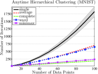
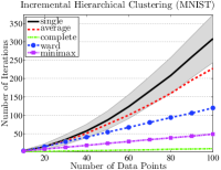
Figure 4: Average number of iterations of anytime (left) and incremental (right) hierarchical clusterings for the MNIST dataset. Shaded regions illustrate the sample variance for the single linkage.

Using an empirical evaluation of anytime and incremental hierarchical clustering methods we aim to statistically explore: (1) the number of iterations of anytime and incremental clusterings, and (2) their effectiveness compared to the traditional agglomerative clustering methods.

As expected, the number of iterations to homogeneous termination of any anytime clustering depends strongly on the initial conditions (i.e, the initial pair of dataset and tree). To challenge the proposed clustering method, we always start anytime clustering of a dataset at a random initial clustering hierarchy uniformly sampled from the space of non-degenerate hierarchies [36]. To give some preliminary idea of performance as a function of data size we run the various methods on datasets of cardinality $10,20,\ldots,100,$ and report statistics from the results of $1000$ different randomly selected pairings of initial data set and tree using both synthetic and real data collections generated as described in Section 5.1.

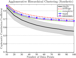
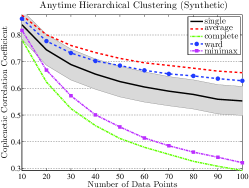
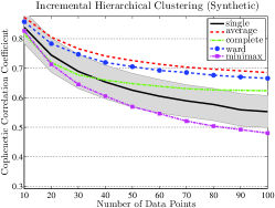
Figure 5: Average cophenetic correlation coefficient for agglomerative (left), anytime (middle) and incremental (right) hierarchical clusterings of simulated data points. Shaded regions illustrate the sample variance for the single linkage.

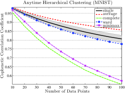
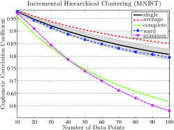
Figure 6: Average cophenetic correlation coefficient for agglomerative (left), anytime (middle) and incremental (right) hierarchical clusterings for the MNIST dataset. Shaded regions illustrate the sample variance for the single linkage.

For each linkage function discussed in Section 2.4.1, Figure 12 and Figure 12 present the average number of iterations of anytime and incremental clusterings versus the dataset size. Regardless of linkage and size, incremental clustering generally requires an order of magnitude fewer iterations than does anytime clustering. This is a consequence of our experimental design whereby anytime clustering is always initialized from a random clustering tree while incremental clustering takes the advantage of local homogeneity for effective insertion of a new datum into an existing clustering tree. The next clearest pattern that emerges from these figures is that the number of iterations for both anytime and incremental clustering methods seems to grow quite differently for single linkage (where it appears quadratic in the size of the dataset) than for other familiar linkages (relative to which these preliminary statistics are not inconsistent with linear growth) - but more exploration with larger cardinality datasets will be required before more specific conjectures are possible.

Figure 12 and Figure 12 illustrate how cophenetic correlation coefficient (58) changes with the dataset size for agglomerative, anytime and incremental hierarchical clustering methods. Recall from Theorem 3.6 that a clustering hierarchy resulting from agglomerative single linkage clustering of a dataset is uniquely characterised by its homogeneity relative to single linkage. Hence, it must be the case (as is indeed reflected in these figures) that the clustering performance of single linkage clustering is the same for all agglomerative, anytime and incremental methods. Here, assuming the results of agglomerative clustering as the ground truth, anytime and incremental clusterings using complete and minimax linkages is observed to perform relatively poorly, which is probably due to their overestimation of cluster dissimilarities. On the other hand, for average and Ward’s linkages anytime and incremental hierarchical clusterings perform as well as agglomerative clustering. Further, as expected, incremental clustering generally performs better than anytime clustering since it uses local homogeneity to properly insert each new data point and calls anytime clustering starting at a clustering tree which is far better than a random hierarchy. Finally, one can notice that the clustering performance of all hierarchical methods is better on real datasets than synthetic datasets, which is likely due to increased dimensionality and sparsity of data as discussed in Section 5.1.

6 Conclusions

In this paper, we introduce a new homogeneity criterion (Definition 4), for a clustering tree associated with a data set applicable to a reasonably broad subclass of the familiar linkage functions. We show that homogeneity is a characteristic property of trees resulting from any such standard (linkage based) hierarchical clustering methods (Proposition 3.4). In particular, homogeneity uniquely characterizes the single linkage clustering tree of a data set (Theorem 3.6).

We propose an anytime hierarchical clustering method in Table 3 that iteratively transforms any initial clustering hierarchy into a homogeneous clustering tree of a dataset relative to a user-specified linkage function. For the subclass of linkages (specified in Definition 4.8 — including single, complete, minimax and Ward’s linkages) we demonstrate that this iterative clustering procedure must terminate in finite time (Theorem 4.11). Finally , we discuss certain settings for computationally efficient anytime clustering and describe an incremental hierarchical clustering method based on local homogeneity of cluster trees and anytime clustering.

The “anytime" nature of our method enables users to choose between accuracy and efficiency. In contrast to batch methods, any intermediate stage of anytime hierarchical clustering returns a valid clustering tree and incrementally improves the homogeneity at each iteration. Thus, at any time a user can stop clustering and continue it later with or without updating the data set. Further, since our method is based on local tree restructuring (the familiar NNI-walk, Definition 1 [33, 28]), it provides an opportunity for distributed/parallel implementation and reactive tracking. The experimental evaluation of sample anytime and incremental hierarchical clustering approaches suggested by these new ideas suggests their value relative to the standard “batch" methods.

Work is presently in progress to establish bounds on the number of iterations of anytime and incremental hierarchical clustering methods, and to develop specific implementations for efficient computation of anytime clustering. In the longer term, we believe these ideas will extend to a randomized algorithm for anytime single linkage clustering as well as to settings where simultaneous distance metric learning must take place in parallel with the hierarchical clustering process.

7 Acknowledgement

This work was funded in part by the Air Force Office of Science Research under the MURI FA9550-10-1-0567.

Appendix A Sum of Ward’s Linkages & Sum of Squared Error

Although sums of linkage values $H_{\mathrm{\mathbf{x}},\zeta}$ (36) of distinct clustering hierarchies associated with a set of data points $\mathrm{\mathbf{x}}\in{\rm Phys.~{}Rev.~{}Lett.}{\mathbb{R}^{m}}^{J}$ and a linkage function $\zeta$ generally differ, $H_{\mathrm{\mathbf{x}},\zeta_{W}}$ is constant for Ward’s linkage $\zeta_{W}$ (10e):

Lemma A.13.

The sum of linkage values $H_{\mathrm{\mathbf{x}},\zeta_{W}}$(36) of any clustering hierarchy associated with a data set $\mathrm{\mathbf{x}}\in{\rm Phys.~{}Rev.~{}Lett.}{\mathbb{R}^{m}}^{J}$ and Ward’s linkage $\zeta_{W}$ (10e) is constant and equal to the sum of squared errors of $\mathrm{\mathbf{x}}$, i.e. for any $\tau\in\mathcal{BT}_{J}$

$$H_{\mathrm{\mathbf{x}},\zeta_{W}}{\rm Phys.~{}Rev.~{}Lett.}{\tau}=\mathrm{SSE}{\rm Phys.~{}Rev.~{}Lett.}{\mathrm{\mathbf{x}}},$$ (59)

where

$$\mathrm{SSE}{\rm Phys.~{}Rev.~{}Lett.}{\mathrm{\mathbf{x}}}\>{\mathbf{:}=}\>\sum_{i\in J}\left\|\mathrm{x}_{i}-\mathrm{c}{\rm Phys.~{}Rev.~{}Lett.}{\mathrm{\mathbf{x}}|J}\right\|_{2}^{2}.$$ (60)

Proof A.14.

Recall from [38, 22] that Ward’s linkage quantifies the change in the sum of squared errors after merging a group of data points, i.e. for any $\mathrm{\mathbf{x}}\in{\rm Phys.~{}Rev.~{}Lett.}{\mathbb{R}^{m}}^{J}$ and disjoint subsets $A,B\subseteq J$

$$\zeta_{W}{\rm Phys.~{}Rev.~{}Lett.}{\mathrm{\mathbf{x}};A,B}=\mathrm{SSE}{\rm Phys.~{}Rev.~{}Lett.}{\mathrm{\mathbf{x}}|A\!\cup\!B}\!-\!\mathrm{SSE}{\rm Phys.~{}Rev.~{}Lett.}{\mathrm{\mathbf{x}}|A}\!-\!\mathrm{SSE}{\rm Phys.~{}Rev.~{}Lett.}{\mathrm{\mathbf{x}}|B}\!.\!\!$$ (61)

Let $\tau\in\mathcal{BT}_{J}$ be a binary hierarchy with the root split $\left\{J_{L},J_{R}\right\}=\mathrm{Ch}{\rm Phys.~{}Rev.~{}Lett.}{J,\tau}$. Proof by induction.

• (Base Case) if $\left|J\right|=2$, then there is only one clustering hierarchy $\tau\in\mathcal{BT}_{\left[2\right]}$, i.e. $\left|\mathcal{BT}_{\left[2\right]}\right|=1$. Note that $\tau$ only has one Ward’s linkage joining two data points of $\mathrm{\mathbf{x}}={\rm Phys.~{}Rev.~{}Lett.}{\mathrm{x}_{1},\mathrm{x}_{2}}$ whose value equals to the sum of squared errors of $\mathrm{\mathbf{x}}$,

  $$H_{\mathrm{\mathbf{x}},\zeta_{W}}{\rm Phys.~{}Rev.~{}Lett.}{\tau} =\zeta_{W}{\rm Phys.~{}Rev.~{}Lett.}{\mathrm{\mathbf{x}};\left\{1\right\},\left\{2\right\}}=\frac{1}{2}\left\|\mathrm{x}_{1}-\mathrm{x}_{2}\right\|_{2}^{2},$$ (62)

  $$=\!\!\sum_{i\in\left\{1,2\right\}}\left\|\mathrm{x}_{i}-\mathrm{c}{\rm Phys.~{}Rev.~{}Lett.}{\mathrm{\mathbf{x}}|\left\{1,2\right\}}\right\|_{2}^{2}=\mathrm{SSE}{\rm Phys.~{}Rev.~{}Lett.}{\mathrm{\mathbf{x}}}\!.\!\!$$ (63)

• (Induction) Let $\tau_{L}$ and $\tau_{R}$ denote the subtrees of $\tau$ rooted at $J_{L}$ and $J_{R}$, respectively. Suppose that

  $$H_{\mathrm{\mathbf{x}}|J_{L},\zeta_{W}}{\rm Phys.~{}Rev.~{}Lett.}{\tau_{L}}=\mathrm{SSE}{\rm Phys.~{}Rev.~{}Lett.}{\mathrm{\mathbf{x}}|J_{L}},$$ (64)

  $$H_{\mathrm{\mathbf{x}}|J_{R},\zeta_{W}}{\rm Phys.~{}Rev.~{}Lett.}{\tau_{R}}=\mathrm{SSE}{\rm Phys.~{}Rev.~{}Lett.}{\mathrm{\mathbf{x}}|J_{R}}.$$ (65)

  Note that if any of subtrees only has one leaf, e.g. $\left|J_{L}\right|=1$ , then we set the associated sum of linkage values to zero, $H_{\mathrm{\mathbf{x}}|J_{L},\zeta_{W}}{\rm Phys.~{}Rev.~{}Lett.}{\tau_{L}}=0$.

  Hence, using (61), one can obtain the result as follows:

  $$H_{\mathrm{\mathbf{x}},\zeta_{W}}\!{\rm Phys.~{}Rev.~{}Lett.}{\tau} \!=\!H_{\mathrm{\mathbf{x}}|J_{L}\!,\zeta_{W}}\!{\rm Phys.~{}Rev.~{}Lett.}{\tau_{L}}\!+\!H_{\mathrm{\mathbf{x}}|J_{R}\!,\zeta_{W}}\!{\rm Phys.~{}Rev.~{}Lett.}{\tau_{R}}\!+\!\zeta_{W}\!{\rm Phys.~{}Rev.~{}Lett.}{\mathrm{\mathbf{x}};\!J_{L},\!J_{R}}\!,\!\!$$ (66)

  $$\!=\!\mathrm{SSE}{\rm Phys.~{}Rev.~{}Lett.}{\mathrm{\mathbf{x}}|J_{L}}\!+\!\mathrm{SSE}{\rm Phys.~{}Rev.~{}Lett.}{\mathrm{\mathbf{x}}|J_{R}}+\zeta_{W}\!{\rm Phys.~{}Rev.~{}Lett.}{\mathrm{\mathbf{x}};\!J_{L},\!J_{R}}\!,\!\!$$ (67)

  $$\!=\!\mathrm{SSE}{\rm Phys.~{}Rev.~{}Lett.}{\mathrm{\mathbf{x}}}.$$ (68)

Appendix B Termination Analysis for
Average Linkage

Lemma B.15.

Iterated application of Anytime Hierarchical $\zeta_{A}$-Clustering procedure in Table 3 initiated from any clustering tree in $\mathcal{BT}_{J}$ for a fixed set of data points $\mathrm{\mathbf{x}}\in{\rm Phys.~{}Rev.~{}Lett.}{\mathbb{R}^{m}}^{J}$ terminates in finite time at a clustering hierarchy in $\mathcal{BT}_{J}$ that is homogeneous relative to average linkage $\zeta_{A}$ (10c).

Proof B.16.

As in the proof of more general result in Theorem 4.11, we shall show that the anytime clustering rule does not cause any cycle in $\mathcal{BT}_{J}$ before terminating at a structurally homogeneous clustering hierarchy. Consequently, the finite time termination of the anytime clustering method is simply due to finiteness of tree space $\mathcal{BT}_{J}$ (5).

Let $S{\rm Phys.~{}Rev.~{}Lett.}{\tau}$ denote the ordered set of linkage values of a binary clustering hierarchy $\tau\in\mathcal{BT}_{J}$ associated with $\mathrm{\mathbf{x}}$ and $\zeta_{A}$ in ascending order, i.e.

$$S{\rm Phys.~{}Rev.~{}Lett.}{\tau} \>{\mathbf{:}=}\>{\rm Phys.~{}Rev.~{}Lett.}{\Big{.}\zeta_{A}{\rm Phys.~{}Rev.~{}Lett.}{\mathrm{\mathbf{x}};I,{I}^{-\tau}}}_{I\in\mathscr{C}\left(\tau\right)},$$ (69)

$$S{\rm Phys.~{}Rev.~{}Lett.}{\tau}_{i} \leq S{\rm Phys.~{}Rev.~{}Lett.}{\tau}_{j},\quad\forall\;1\leq i\leq j\leq 2\left|J\right|-1,$$ (70)

where $S{\rm Phys.~{}Rev.~{}Lett.}{\tau}={\rm Phys.~{}Rev.~{}Lett.}{\!S{\rm Phys.~{}Rev.~{}Lett.}{\tau}_{1}\!,S{\rm Phys.~{}Rev.~{}Lett.}{\tau}_{2}\!,\ldots,S{\rm Phys.~{}Rev.~{}Lett.}{\tau}_{2\left|J\right|-1}\!}$ and note that the number of clusters of a binary tree over leaf set $J$ is $2\left|J\right|-1$ [35]. Further, have the set of $\;{\rm Phys.~{}Rev.~{}Lett.}{2\left|J\right|-1}$-tuple of real numbers ordered lexicographically according to the standard order of reals.

Let $\tau^{k}\in\mathcal{BT}_{J}$ be a clustering hierarchy visited at $k$-th iteration of anytime hierarchical clustering of $\mathrm{\mathbf{x}}$, where $k\geq 0$. To prove the result, we shall show the following

$$S{\rm Phys.~{}Rev.~{}Lett.}{\tau^{k}}>S{\rm Phys.~{}Rev.~{}Lett.}{\tau^{k+1}}.$$ (71)

Since $\tau^{k}$ and $\tau^{k+1}$ are NNI-adjacent, let ${\rm Phys.~{}Rev.~{}Lett.}{A^{k},B^{k},C^{k}}$ be the NNI-triplet (Lemma 1) associated with the pair of ${\rm Phys.~{}Rev.~{}Lett.}{\tau^{k},\tau^{k+1}}$. Recall that $A^{k}\cup B^{k}\in\mathscr{C}\left(\tau^{k}\right)\setminus\mathscr{C}\left(\tau^{k+1}\right)$ and $B^{k}\cup C^{k}\in\mathscr{C}\left(\tau^{k+1}\right)\setminus\mathscr{C}\left(\tau^{k}\right)$.

Note that after the NNI transition from $\tau^{k}$ to $\tau^{k+1}$ two elements of $S{\rm Phys.~{}Rev.~{}Lett.}{\tau^{k}}$, $\zeta_{A}\!{\rm Phys.~{}Rev.~{}Lett.}{\mathrm{\mathbf{x}};\!A^{k}\!,\!B^{k}\!}$ and $\zeta_{A}\!{\rm Phys.~{}Rev.~{}Lett.}{\mathrm{\mathbf{x}};\!A^{k}\!\cup\!B^{k}\!,\!C^{k}\!}$, are replaced by another two reals, $\zeta_{A}\!{\rm Phys.~{}Rev.~{}Lett.}{\mathrm{\mathbf{x}};\!B^{k}\!,C^{k}\!}$ and $\zeta_{A}\!{\rm Phys.~{}Rev.~{}Lett.}{\mathrm{\mathbf{x}};\!B^{k}\!\cup\!C^{k}\!,\!A^{k}\!}$, to yield $S{\rm Phys.~{}Rev.~{}Lett.}{\tau^{k+1}}$.

By construction of the anytime clustering rule, we have

$$\zeta_{A}{\rm Phys.~{}Rev.~{}Lett.}{\mathrm{\mathbf{x}};A^{k},B^{k}} >\zeta_{A}{\rm Phys.~{}Rev.~{}Lett.}{\mathrm{\mathbf{x}};B^{k},C^{k}},$$ (72)

$$\zeta_{A}{\rm Phys.~{}Rev.~{}Lett.}{\mathrm{\mathbf{x}};A^{k},C^{k}} \geq\zeta_{A}{\rm Phys.~{}Rev.~{}Lett.}{\mathrm{\mathbf{x}};B^{k},C^{k}},$$ (73)

and, using the definition of average linkage (10c), one can verify that

$$\zeta_{A}{\rm Phys.~{}Rev.~{}Lett.}{\mathrm{\mathbf{x}};A^{k}\cup B^{k},C^{k}}\geq\zeta{\rm Phys.~{}Rev.~{}Lett.}{\mathrm{\mathbf{x}};B^{k},C^{k}}.$$ (74)

If $\zeta_{A}{\rm Phys.~{}Rev.~{}Lett.}{\mathrm{\mathbf{x}};A^{k}\cup B^{k},C^{k}}>\zeta_{A}{\rm Phys.~{}Rev.~{}Lett.}{\mathrm{\mathbf{x}};B^{k},C^{k}}$, then it is clear from (72) and (10c) that

$$\min{\rm Phys.~{}Rev.~{}Lett.}{\big{.}\!\zeta_{A}\!{\rm Phys.~{}Rev.~{}Lett.}{\!\mathrm{\mathbf{x}};\!A^{k}\!,\!B^{k}\!}\!,\zeta_{A}\!{\rm Phys.~{}Rev.~{}Lett.}{\!\mathrm{\mathbf{x}};\!A^{k}\!\cup\!B^{k}\!,\!C^{k}\!}\!\!} \!>\!\zeta_{A}\!{\rm Phys.~{}Rev.~{}Lett.}{\mathrm{\mathbf{x}};\!B^{k},\!C^{k}\!},$$ (75)

$$\!=\!\min{\rm Phys.~{}Rev.~{}Lett.}{\big{.}\!\zeta_{A}\!{\rm Phys.~{}Rev.~{}Lett.}{\!\mathrm{\mathbf{x}};\!B^{k}\!,\!C^{k}\!}\!\!,\zeta_{A}\!{\rm Phys.~{}Rev.~{}Lett.}{\!\mathrm{\mathbf{x}};\!B^{k}\!\cup\!C^{k}\!,\!A^{k}\!}\!\!}\!\!.\!\!$$ (76)

Otherwise ${\rm Phys.~{}Rev.~{}Lett.}{\zeta_{A}{\rm Phys.~{}Rev.~{}Lett.}{\mathrm{\mathbf{x}};A^{k}\cup B^{k},C^{k}}=\zeta_{A}{\rm Phys.~{}Rev.~{}Lett.}{\mathrm{\mathbf{x}};B^{k},C^{k}}}$, by definition (10c), we have $\zeta_{A}{\rm Phys.~{}Rev.~{}Lett.}{\mathrm{\mathbf{x}};B^{k},C^{k}}=\zeta_{A}{\rm Phys.~{}Rev.~{}Lett.}{\mathrm{\mathbf{x}};A^{k},C^{k}}$, and so $\zeta_{A}{\rm Phys.~{}Rev.~{}Lett.}{\mathrm{\mathbf{x}};A^{k},B^{k}}>\zeta_{A}{\rm Phys.~{}Rev.~{}Lett.}{\mathrm{\mathbf{x}};B^{k}\cup C^{k},A^{k}}$.

In overall, the minimum of changed linkage values at each iteration of anytime clustering strictly decreases, which proves (71) and completes the proof. ∎

Appendix C Special Cases of Average Linkage

We now consider certain settings of average linkage $\zeta_{A}$ (10c) that enables efficient computation of linkage values of a clustering hierarchy and its restructuring during online clustering.

Consider the squared Euclidean distance as a dissimilarity measure of a pair of data points, i.e. for any $\mathrm{x},\mathrm{y}\in\mathbb{R}^{m}$

$$\mathit{d}{\rm Phys.~{}Rev.~{}Lett.}{\mathrm{x},\mathrm{y}}=\left\|\mathrm{x}-\mathrm{y}\right\|_{2}^{2}.$$ (77)

For any $\mathrm{\mathbf{x}}\in{\rm Phys.~{}Rev.~{}Lett.}{\mathbb{R}^{d}}^{J}$ and disjoint subsets $A,B\subseteq J$, the average linkage $\zeta_{A}$ (10c) between partial patterns $\mathrm{\mathbf{x}}|A$ and $\mathrm{\mathbf{x}}|B$, based on the squared Euclidean distance, is

$$\zeta_{A}{\rm Phys.~{}Rev.~{}Lett.}{\mathrm{\mathbf{x}};A,B} \!=\!\frac{1}{\left|A\right|\left|B\right|}\sum_{\begin{subarray}{c}a\in A\\ b\in B\end{subarray}}\!\mathit{d}{\rm Phys.~{}Rev.~{}Lett.}{\mathrm{x}_{a},\mathrm{x}_{b}}\!=\!\frac{1}{\left|A\right|\left|B\right|}\sum_{\begin{subarray}{c}a\in A\\ b\in B\end{subarray}}\!\left\|\mathrm{x}_{a}\!-\!\mathrm{x}_{b}\right\|_{2}^{2}\!,\!\!$$ (78)

$$=\frac{1}{\left|A\right|\left|B\right|}\sum_{\begin{subarray}{c}a\in A\\ b\in B\end{subarray}}\left\|\mathrm{x}_{a}-\mathrm{c}{\rm Phys.~{}Rev.~{}Lett.}{\mathrm{\mathbf{x}}|B}+\mathrm{c}{\rm Phys.~{}Rev.~{}Lett.}{\mathrm{\mathbf{x}}|B}-\mathrm{x}_{b}\right\|_{2}^{2}.$$ (79)

After expanding the norm, (79) simplifies to

$$\zeta_{A}\!{\rm Phys.~{}Rev.~{}Lett.}{\mathrm{\mathbf{x}};\!A,\!B} \!=\!\frac{1}{\left|A\right|}\!\sum_{a\in A}\!\left\|\mathrm{x}_{a}\!-\!\mathrm{c}{\rm Phys.~{}Rev.~{}Lett.}{\mathrm{\mathbf{x}}|B}\right\|_{2}^{2}\!+\!\frac{1}{\left|B\right|}\!\sum_{\begin{subarray}{c}b\in B\end{subarray}}\!\left\|\mathrm{x}_{b}\!-\!\mathrm{c}{\rm Phys.~{}Rev.~{}Lett.}{\mathrm{\mathbf{x}}|B}\right\|_{2}^{2}\!,\!\!\!$$ (80)

$$=\frac{1}{\left|A\right|}\!\sum_{a\in A}\left\|\mathrm{x}_{a}\!-\!\mathrm{c}{\rm Phys.~{}Rev.~{}Lett.}{\mathrm{\mathbf{x}}|A}\!+\!\mathrm{c}{\rm Phys.~{}Rev.~{}Lett.}{\mathrm{\mathbf{x}}|A}\!-\!\mathrm{c}{\rm Phys.~{}Rev.~{}Lett.}{\mathrm{\mathbf{x}}|B}\right\|_{2}^{2}\!+\!\mathrm{v}{\rm Phys.~{}Rev.~{}Lett.}{\mathrm{\mathbf{x}}|B}\!.\!\!\!$$ (81)

Using a similar trick on (81), one can conclude that the value of average linkage between $\mathrm{\mathbf{x}}|A$ and $\mathrm{\mathbf{x}}|B$ is a simple function of their centroids and variances,

$$\zeta_{A}\!{\rm Phys.~{}Rev.~{}Lett.}{\mathrm{\mathbf{x}};\!A,\!B}\!=\!\mathrm{v}{\rm Phys.~{}Rev.~{}Lett.}{\mathrm{\mathbf{x}}|A}+\mathrm{v}{\rm Phys.~{}Rev.~{}Lett.}{\mathrm{\mathbf{x}}|B}+\left\|\mathrm{c}{\rm Phys.~{}Rev.~{}Lett.}{\mathrm{\mathbf{x}}|A}-\mathrm{c}{\rm Phys.~{}Rev.~{}Lett.}{\mathrm{\mathbf{x}}|B}\right\|_{2}^{2}.$$ (82)

where for any $I\subseteq J\;$ $\mathrm{c}{\rm Phys.~{}Rev.~{}Lett.}{\mathrm{\mathbf{x}}|I}$(1) and $\mathrm{v}{\rm Phys.~{}Rev.~{}Lett.}{\mathrm{\mathbf{x}}|I}$(2) denote the centroid and variance of $\mathrm{\mathbf{x}}|I$, respectively.

A similar computational improvement for average linkage is also possible with the cosine dissimilarity — another commonly used dissimilarity, in information retrieval and text mining [34]: for any $\mathrm{x},\mathrm{y}\in\mathbb{R}^{m}$,

$$\mathit{d}{\rm Phys.~{}Rev.~{}Lett.}{\mathrm{x},\mathrm{y}}=1-\frac{\mathrm{x}\cdot\mathrm{y}}{\left\|\mathrm{x}\right\|_{2}\left\|\mathrm{y}\right\|_{2}},$$ (83)

where $\cdot$ denote the Euclidean dot product. For any dataset of unit length vectors $\mathrm{\mathbf{x}}\in{\rm Phys.~{}Rev.~{}Lett.}{\mathbb{S}^{m-1}}^{J}$ and disjoint subsets $A,B\subseteq J$, the average linkage $\zeta_{A}$ (10c) between $\mathrm{\mathbf{x}}|A$ and $\mathrm{\mathbf{x}}|B$, based on the cosine dissimilarity, can be rewritten as

$$\zeta_{A}{\rm Phys.~{}Rev.~{}Lett.}{\mathrm{\mathbf{x}};\!A,\!B} \!=\!\frac{1}{\left|A\right|\!\left|B\right|}\!\sum_{\begin{subarray}{c}a\in A\\ b\in B\end{subarray}}\!\!\mathit{d}{\rm Phys.~{}Rev.~{}Lett.}{\mathrm{x}_{a},\mathrm{x}_{b}}\!=\!\frac{1}{\left|A\right|\!\left|B\right|}\!\sum_{\begin{subarray}{c}a\in A\\ b\in B\end{subarray}}\!1\!-\!\!\!\!\underbrace{\frac{\mathrm{x}_{a}\cdot\mathrm{x}_{b}}{\left\|\mathrm{x}_{a}\right\|_{2}\!\left\|\mathrm{x}_{b}\right\|_{2}}}_{\left\|\mathrm{x}_{a}\right\|_{2}=\left\|\mathrm{x}_{b}\right\|_{2}=1}\!\!,\!\!$$

$$\!=\!1\!-\!\frac{1}{\left|A\right|\!\left|B\right|}\!\sum_{\begin{subarray}{c}a\in A\\ b\in B\end{subarray}}\!\mathrm{x}_{a}\cdot\mathrm{x}_{b}\!=\!1-\mathrm{c}{\rm Phys.~{}Rev.~{}Lett.}{\mathrm{\mathbf{x}}|A}\cdot\mathrm{c}{\rm Phys.~{}Rev.~{}Lett.}{\mathrm{\mathbf{x}}|B},$$ (84)

which directly follows the linearity of the dot product.

Appendix D Sample Variance and Mean
After Merging Clusters

It is well know that for any $\mathrm{\mathbf{x}}\in{\rm Phys.~{}Rev.~{}Lett.}{\mathbb{R}^{d}}^{J}$ and any disjoint subsets $A,B\subseteq J$ of a finite index set $J$, the centroid of merged patterns $\mathrm{\mathbf{x}}|A\cup B$ is simply equal to the weighted average, proportional to the cardinality of sets, of centroids of partial patterns $\mathrm{\mathbf{x}}|A$ and $\mathrm{\mathbf{x}}|B$,

$$\mathrm{c}{\rm Phys.~{}Rev.~{}Lett.}{\mathrm{\mathbf{x}}|A\cup B}=\frac{\left|A\right|}{\left|A\right|+\left|B\right|}\mathrm{c}{\rm Phys.~{}Rev.~{}Lett.}{\mathrm{\mathbf{x}}|A}+\frac{\left|B\right|}{\left|A\right|+\left|B\right|}\mathrm{c}{\rm Phys.~{}Rev.~{}Lett.}{\mathrm{\mathbf{x}}|B}.$$ (85)

Similarly, using (61), one can verify that for any disjoint subsets $A,B\subseteq J$ and $\mathrm{\mathbf{x}}\in{\rm Phys.~{}Rev.~{}Lett.}{\mathbb{R}^{d}}^{J}$, the variance of merged patterns $\mathrm{\mathbf{x}}|A\cup B$ is given by

$$\mathrm{v}{\rm Phys.~{}Rev.~{}Lett.}{\mathrm{\mathbf{x}}|A\!\cup\!B} \!=\!\frac{\left|A\right|}{\left|A\right|\!+\!\left|B\right|}\mathrm{v}{\rm Phys.~{}Rev.~{}Lett.}{\mathrm{\mathbf{x}}|A}\!+\!\frac{\left|B\right|}{\left|A\right|\!+\!\left|B\right|}\mathrm{v}{\rm Phys.~{}Rev.~{}Lett.}{\mathrm{\mathbf{x}}|B}$$

$$\hskip 42.67912pt\!+\!\frac{\left|A\right|\left|B\right|}{{\rm Phys.~{}Rev.~{}Lett.}{\left|A\right|\!+\!\left|B\right|}^{2}}\!\left\|\big{.}\mathrm{c}{\rm Phys.~{}Rev.~{}Lett.}{\mathrm{\mathbf{x}}|A}\!-\!\mathrm{c}{\rm Phys.~{}Rev.~{}Lett.}{\mathrm{\mathbf{x}}|B}\right\|_{2}^{2}.$$ (86)

References

- [1] E. Achtert, C. Bohm, H.-P. Kriegel, and P. Kroger. Online hierarchical clustering in a data warehouse environment. In Data Mining, Fifth IEEE International Conference on, pages 8–pp. IEEE, 2005.
- [2] M. Ackerman, S. Ben-David, and D. Loker. Characterization of linkage-based clustering. In COLT, pages 270–281, 2010.
- [3] C. C. Aggarwal, J. Han, J. Wang, and P. S. Yu. A framework for clustering evolving data streams. In Proceedings of the 29th international conference on Very large data bases, pages 81–92. VLDB Endowment, 2003.
- [4] O. Arslan, D. Guralnik, and D. E. Koditschek. Discriminative measures for comparison of phylogenetic trees. Technical report, University Of Pennsylvania, 2013. http://arxiv.org/abs/1310.5202.
- [5] P. Berkhin. A survey of clustering data mining techniques. In Grouping multidimensional data, pages 25–71. Springer, 2006.
- [6] J. Bien and R. Tibshirani. Hierarchical clustering with prototypes via minimax linkage. Journal of the American Statistical Association, 106(495):1075–1084, 2011.
- [7] L. J. Billera, S. P. Holmes, and K. Vogtmann. Geometry of the space of phylogenetic trees. Advances in Applied Mathematics, 27(4):733–767, 2001.
- [8] P. S. Bradley, U. M. Fayyad, and C. Reina. Scaling clustering algorithms to large databases. In Proceedings of the fourth ACM SIGKDD international conference on Knowledge discovery and data mining, pages 9–15, 1998.
- [9] M. M. Breunig, H.-P. Kriegel, P. Kröger, and J. Sander. Data bubbles: Quality preserving performance boosting for hierarchical clustering. SIGMOD Rec., 30(2):79–90, 2001.
- [10] M. Bruynooghe. Classification ascendante hiérarchique des grands ensembles de données: un algorithme rapide fondé sur la construction des voisinages réductibles. Cahiers de l’Analyse des Données, 3(1):7–33, 1978.
- [11] G. Carlsson and F. Mémoli. Characterization, Stability and Convergence of Hierarchical Clustering methods. Journal of Machine Learning Research, 11:1425–1470, 2010.
- [12] W. DuMouchel, C. Volinsky, T. Johnson, C. Cortes, and D. Pregibon. Squashing flat files flatter. In Proceedings of the fifth ACM SIGKDD international conference on Knowledge discovery and data mining, pages 6–15. ACM, 1999.
- [13] J. Felsenstein. Inferring Phylogenies. Sinauer Associates, Suderland, USA, 2004.
- [14] D. H. Fisher. Knowledge acquisition via incremental conceptual clustering. Machine learning, 2(2):139–172, 1987.
- [15] R. G. Gallager, P. A. Humblet, and P. M. Spira. A distributed algorithm for minimum-weight spanning trees. ACM Transactions on Programming Languages and systems (TOPLAS), 5(1):66–77, 1983.
- [16] A. D. Gordon. A review of hierarchical classification. Journal of the Royal Statistical Society. Series A (General), pages 119–137, 1987.
- [17] J. C. Gower and G. J. S. Ross. Minimum Spanning Trees and Single Linkage Cluster Analysis. Journal of the Royal Statistical Society. Series C (Applied Statistics), 18(1), 1969.
- [18] S. Guha, A. Meyerson, N. Mishra, R. Motwani, and L. O’Callaghan. Clustering data streams: Theory and practice. Knowledge and Data Engineering, IEEE Transactions on, 15(3):515–528, May 2003.
- [19] S. Guha, R. Rastogi, and K. Shim. Cure: an efficient clustering algorithm for large databases. Information Systems, 26(1):35–58, 2001.
- [20] J. Han, M. Kamber, and J. Pei. Data mining: concepts and techniques. Morgan Kaufmann, 2006.
- [21] T. Hastie, R. Tibshirani, and J. Friedman. The elements of statistical learning. Springer Series in Statistics. Springer, New York, NY, USA, 2009.
- [22] A. K. Jain and R. C. Dubes. Algorithms for clustering data. Prentice-Hall, Inc., 1988.
- [23] A. K. Jain, M. N. Murty, and P. J. Flynn. Data clustering: a review. ACM computing surveys (CSUR), 31(3):264–323, 1999.
- [24] G. Karypis, E.-H. Han, and V. Kumar. Chameleon: Hierarchical clustering using dynamic modeling. Computer, 32(8):68–75, 1999.
- [25] G. N. Lance and W. T. Williams. A general theory of classificatory sorting strategies 1. hierarchical systems. The Computer Journal, 9(4):373–380, 1967.
- [26] Y. LeCun, L. Bottou, Y. Bengio, and P. Haffner. Gradient-based learning applied to document recognition. Proceedings of the IEEE, 86(11):2278–2324, 1998.
- [27] B. Mirkin. Mathematical Classification and Clustering. Kluwer Academic Publishers, 1996.
- [28] G. Moore, M. Goodman, and J. Barnabas. An iterative approach from the standpoint of the additive hypothesis to the dendrogram problem posed by molecular data sets. Journal of Theoretical Biology, 38(3):423–457, 1973.
- [29] F. Murtagh. A survey of recent advances in hierarchical clustering algorithms. The Computer Journal, 26(4):354–359, 1983.
- [30] F. Murtagh. The remarkable simplicity of very high dimensional data: Application of model-based clustering. Journal of Classification, 26(3):249–277, 2009.
- [31] R. T. Ng and J. Han. Clarans: A method for clustering objects for spatial data mining. Knowledge and Data Engineering, IEEE Transactions on, 14(5):1003–1016, 2002.
- [32] C. F. Olson. Parallel algorithms for hierarchical clustering. Parallel computing, 21(8):1313–1325, 1995.
- [33] D. Robinson. Comparison of labeled trees with valency three. Journal of Combinatorial Theory, Series B, 11(2):105–119, 1971.
- [34] G. Salton and C. Buckley. Term-weighting approaches in automatic text retrieval. Information Processing & Management, 24(5):513 – 523, 1988.
- [35] A. Schrijver. Combinatorial optimization: polyhedra and efficiency, volume 24. Springer, 2003.
- [36] C. Semple and M. Steel. Phylogenetics, volume 24. Oxford University Press, 2003.
- [37] R. R. Sokal and F. J. Rohlf. The comparison of dendrograms by objective methods. Taxon, 11(2):33–40, 1962.
- [38] J. H. Ward Jr. Hierarchical grouping to optimize an objective function. Journal of the American Statistical Association, 58(301):236–244, 1963.
- [39] D. Widyantoro, T. Ioerger, and J. Yen. An incremental approach to building a cluster hierarchy. In Data Mining, 2002. ICDM 2002. Proceedings. 2002 IEEE International Conference on, pages 705–708, 2002.
- [40] E. P. Xing, M. I. Jordan, S. Russell, and A. Ng. Distance metric learning with application to clustering with side-information. In Advances in Neural Information Processing Systems, pages 505–512, 2002.
- [41] T. Zhang, R. Ramakrishnan, and M. Livny. Birch: An efficient data clustering method for very large databases. SIGMOD Record, 25(2):103–114, 1996.