Date: April 13, 2014

Higher order QCD results for the fermionic contributions of the Higgs-boson decay into two photons and the decoupling function for the $\overline{\mbox{MS}}$ renormalized fine-structure constant

Christian Sturm
Universität Würzburg,
Institut für Theoretische Physik und Astrophysik,
Emil-Hilb-Weg 22,
D-97074 Würzburg,
Germany
Abstract

We compute the decoupling function of the $\overline{\mbox{MS}}$ renormalized fine-structure constant up to four-loop order in perturbative QCD. The results are used in order to determine the related top-quark contributions to the Higgs-boson decay into two photons in the heavy top-quark mass limit to order $\alpha_{s}^{4}$.

1 Introduction

The discovery of a Higgs-particle [1, 2] which is, within the current uncertainties, consistent with the expectations of the Standard Model (SM) Higgs boson ($H$) was a big success of the Large Hadron Collider (LHC) experiments. It is now interesting and important to further understand and study its properties also from theory side.

The dominant production mechanism for the SM Higgs boson at the LHC is the gluon fusion process, whereas the Higgs-boson decay into two photons, $H\to\gamma\gamma$, provides a clean channel for the study of its properties, not only at the LHC, but also at a future linear collider. As a result of this these processes are studied at high order in perturbation theory to obtain most accurate predictions. From theory point of view both reactions are loop induced processes, since the SM Higgs boson couples only to massive particles, so that the leading order processes are here already at the one-loop level. In the limit in which the heavy top-quark mass $m_{t}$ is much larger than the mass of the Higgs boson, $m_{H}\ll 2\*m_{t}$, the fermionic contributions can be described by an effective coupling using a low-energy theorem (LET) [3, 4, 5, 6].

Within this work we study higher order corrections in quantum chromodynamics (QCD) to the decay $H\to\gamma\gamma$. For electroweak corrections we refer to Refs. [7, 8, 9, 10, 11]. The two-loop QCD corrections are known since long and have been determined first in the heavy top-quark mass limit in Refs. [12, 13]. The full top-quark mass dependence has then been obtained numerically and analytically in Refs. [14, 15, 16, 17, 18, 19, 20]. In the following we will focus on the purely fermionic contributions to the decay $H\to\gamma\gamma$ which form a gauge-invariant set of diagrams. We will further distinguish between the singlet and non-singlet contributions. The latter are given by those diagrams for which the Higgs boson and the photons couple to the same top-quark loop. The three-loop QCD corrections of the non-singlet diagrams including power corrections up to $\mathcal{O}((m_{H}^{2}/(4\*m_{t}^{2}))^{2})$ were determined in Ref. [21]. This result was complemented in Ref. [22], where additional power corrections of higher order in $m_{H}^{2}/(4\*m_{t}^{2})$ as well as the complete singlet contribution has been computed. The symbol $m_{H}$ is here the mass of the Higgs boson and $m_{t}$ is the mass of the top quark.

The four-loop QCD corrections induced by a heavy quark were derived in the heavy quark mass limit by using the known results for the $\beta$-function and mass anomalous dimensions in Ref. [23]. In the following we will first compute the QCD corrections to the decoupling function of the QED coupling constant up to four-loop order. This extends the result of Ref. [23] by one order in perturbation theory. As an application we will use this result in order to derive independently the four-loop QCD corrections induced by a heavy quark to the decay $H\to\gamma\gamma$ in the heavy top-quark mass limit by applying the LET, instead of using the anomalous dimensions as in Ref. [23]. In the next step we will in turn exploit the renormalization group equation (RGE) in order to reconstruct the logarithmic part of the vacuum polarization function at five-loop order, which is again sufficient in order to derive the corresponding contributions to the decay amplitude $H\to\gamma\gamma$ to order $\alpha_{s}^{4}$; here $\alpha_{s}$ is the strong coupling constant.

This paper is structured as follows: In the next Section 2 we discuss the generalities and notations which are needed for this work. In Section 3 we describe the calculation and present our results. Finally we close with a short summary in Section 4. In the Appendix we provide supplementary information.

2 Generalities and notation

The partial decay width for the Higgs-boson decay into two photons is at leading order given by

$$\Gamma(H\to\gamma\gamma)={m_{H}^{3}\over 64\*\pi}\*\Big{|}A_{W}(\tau_{W})+\sum_{f}A_{f}(\tau_{f})\Big{|}^{2}\,,$$ (1)

where $A_{W}(\tau_{W})$ is the contribution which arises from purely bosonic diagrams and $A_{f}(\tau_{f})$ is the fermionic contribution to the amplitude, respectively. The symbol $\tau_{i}$ denotes the mass ratio $m_{H}^{2}/(4\*m_{i}^{2})$ ($i=W,f$), where $m_{W}$ is the mass of the $W$-boson and $m_{f}$ is the mass of a heavy fermion. Within this work we focus only on the term $A_{f}(\tau_{f})$, since we will consider QCD at higher order in perturbation theory. In particular the fermionic contribution of the amplitude is dominated by the contribution which originates from the top quark, $A_{t}(\tau_{t})$ ($f=t$), since the top quark is the heaviest fermion of the SM. In the limit of a heavy top-quark mass, $m_{t}\to\infty$, the leading order result for the amplitude reads $\hat{A}_{t}=N_{c}\*{2\*Q_{t}^{2}\*\alpha\over 3\*\pi\*v}$, with $v=2^{-1/4}G_{F}^{-1/2}$. The symbol $N_{c}$ is here the number of colors of $SU(N_{c})$, $Q_{t}$ is the electric charge factor of the top quark, $\alpha$ is the fine-structure constant, and $G_{F}$ is the Fermi-coupling constant. By integrating out the heavy top-quark one can construct a heavy top-quark effective Lagrangian which describes the interactions of the Higgs field $H$ with the photon field and the $n_{l}$ light quark flavors, which are considered as massless

$$\mathcal{L}_{\mbox{\scriptsize{eff}}}=-{H^{0}\over v^{0}}F^{{}^{\prime}0,\mu\nu}F^{{}^{\prime}0}_{\mu\nu}\,C^{0}_{1\gamma}\,.$$ (2)

The symbol $v^{0}$ is the vacuum expectation value and $F^{{}^{\prime}0}_{\mu\nu}$ is the field strength tensor. The subscript $0$ denotes here and in the following a bare quantity and the prime implies quantities in the effective theory with $n_{l}$ light active quark flavors. The coefficient function $C^{0}_{1\gamma}=-{1\over 2}\*m_{t}^{0}{\partial\ln(\zeta_{g\gamma}^{0})\over\partial m_{t}^{0}}$ depends on the decoupling function $\zeta^{0}_{g\gamma}$, which relates, after renormalization, the $\overline{\mbox{MS}}$ renormalized fine-structure constant in the effective and full theory with $n_{f}=n_{l}+1$ active quark flavors: $\overline{\alpha}^{\prime}(\mu)=\zeta^{2}_{g\gamma}\overline{\alpha}^{(n_{f})}(\mu)$. The decoupling function $\zeta^{0}_{g\gamma}$ can be determined by the computation of the hard part of the photon vacuum polarization function $\Pi^{0h}(q^{2},m_{t}^{0})$ at zero momentum, $q^{2}=0$, e. g. by considering only those diagrams which involve the heavy top quark,

$${\zeta^{0}_{g\gamma}}^{2}={1\over 1+\Pi^{0h}(q^{2}=0,m_{t}^{0})}\,.$$ (3)

Fig. 1 shows some example Feynman diagrams which contribute to the calculation of $\Pi^{0h}(q^{2}=0,m_{t}^{0})$.

$Q_{t}^{2}C_{F}^{3}$

$Q_{t}^{2}C_{F}^{2}C_{A}$

$Q_{t}^{2}C_{F}C_{A}^{2}$

$Q_{t}^{2}n_{h}C_{F}^{2}T_{F}$

$Q_{t}^{2}n_{h}C_{F}C_{A}T_{F}$

$Q_{t}^{2}n_{l}C_{F}^{2}T_{F}$

$Q_{t}^{2}n_{l}C_{F}C_{A}T_{F}$

$Q_{t}^{2}n_{l}^{2}C_{F}T_{F}^{2}$

$Q_{t}^{2}n_{h}n_{l}C_{F}T_{F}^{2}$

$Q_{t}^{2}n_{h}^{2}C_{F}T_{F}^{2}$

$Q_{t}^{2}\mbox{si}\,d^{abc}d^{abc}$

$Q_{q}^{2}\,n_{h}C_{F}^{2}T_{F}$

$Q_{q}^{2}\,n_{h}^{2}C_{F}T_{F}^{2}$

$Q_{q}^{2}\,n_{h}C_{F}C_{A}T_{F}$

$Q_{q}^{2}\,n_{h}n_{l}C_{F}T_{F}^{2}$

$Q_{q}\,Q_{t}\,\mbox{si}\,d^{abc}d^{abc}$

Figure 1: For each color structure which appears at four-loop order in the vacuum polarization function $\Pi^{0h}(q^{2}=0,m_{t}^{0})$ one example Feynman graph is shown. The twisted lines denote gluons, the solid lines are heavy top-quarks and the dashed lines represent massless quarks. The number of inserted heavy and light fermion loops as well as the charge factors are given in the subscripts. The color factors are defined in Section 3.

In the following we decompose the hard part of the vacuum polarization function into three contributions:

$$\Pi^{0h}(q^{2}=0,m_{t}^{0})=\Pi_{t}^{0h}(q^{2}=0,m_{t}^{0})+\sum_{i=1}^{n_{l}}\Pi_{q_{i}}^{0h}(q^{2}=0,m_{t}^{0})+\sum_{i=1}^{n_{l}}\Pi_{tq_{i}}^{0h}(q^{2}=0,m_{t}^{0})\,.$$ (4)

The first term $\Pi_{t}^{0h}(q^{2}=0,m_{t}^{0})$ is the part which is proportional to the charge factor $Q_{t}^{2}$ and arises from the diagrams in which the external photons couple only to top quarks. In contrast, the second term $\sum_{i=1}^{n_{l}}\Pi_{q_{i}}^{0h}(q^{2}=0,m_{t}^{0})$ arises starting from three-loop order in QCD from those contributions for which the external photons couple to light quarks with the global charge factor $Q_{q_{i}}^{2}$. The last term arises from singlet diagrams which are characterized by the fact that one photon couples to a light quark loop and the other photon to a massive top-quark loop. This last term is proportional to the charge factors $Q_{t}\*Q_{q_{i}}$ and appears for the first time at four-loop order.

For the decay process $H\to\gamma\gamma$ we will in the following consider only those gauge-invariant contributions for which the photons couple directly to a top-quark loop. Making Eq. (2) explicit one obtains for the effective Higgs-photon-photon coupling the Lagrangian

$$\mathcal{L}_{H\gamma\gamma}=-{1\over 4}F^{0,\mu\nu}F^{0}_{\mu\nu}\,m^{0}_{t}{\partial\over\partial m^{0}_{t}}\Pi_{t}^{0h}(0,m_{t}^{0}){H^{0}\over v^{0}}\,.$$ (5)

As a result of this one can determine from the hard part of the photon vacuum polarization function the leading top-quark contribution of the bare amplitude $A^{0,\infty}_{t}=-{m^{0}_{t}\over v}{\partial\over\partial{m^{0}_{t}}}{\Pi}_{t}^{0h}(0,m^{0}_{t})$. Considering QCD corrections the $\overline{\mbox{MS}}$ renormalized vacuum polarization function obeys the RGE

$$\left[\beta(a_{s})\*{\partial\over\partial a_{s}}+\gamma_{m}\*\overline{m}_{t}\*{\partial\over\partial\overline{m}_{t}}+\mu^{2}\*{\partial\over\partial\mu^{2}}\right]\*\overline{\Pi}_{t}^{0h}(q^{2}=0,\overline{m}_{t},a_{s},\mu)=4\*\pi\*\alpha\*Q_{t}^{2}\*\gamma_{VV}\,,$$ (6)

with $a_{s}={\alpha_{s}^{(n_{f})}(\mu)/\pi}$, where $\alpha_{s}^{(n_{f})}(\mu)$ and $\overline{m}_{t}\equiv\overline{m}_{t}(\mu)$ are the strong coupling constant and the top-quark mass renormalized in the $\overline{\mbox{MS}}$ scheme. Both depend on the renormalization scale $\mu$. Eq. (6) can be used in order to check the scale dependent part of $\overline{\Pi}_{t}^{0h}(q^{2}=0,\overline{m}_{t},a_{s},\mu)$. The anomalous dimension $\gamma_{VV}$ has been computed in Ref. [24] up to five-loop order. The mass anomalous dimension $\gamma_{m}={\partial\ln\overline{m}_{t}\over\partial\ln\mu^{2}}$ as well as the QCD $\beta$-function $\beta={\partial a_{s}\over\partial\ln\mu^{2}}$ are known up to four-loop order in Refs. [25, 26, 27, 28]. Indeed $\beta$, $\gamma_{m}$ and $\gamma_{VV}$ are known at least one order higher in perturbation theory than needed in order to check the $\mu$-dependent part of the vacuum polarization function up to four-loop order. This allows in turn to predict the $\mu$-dependent part of $\overline{\Pi}^{0h}_{t}(q^{2}=0,\overline{m}_{t})$ at five-loop order from Eq. (6). The $\mu$-independent part, however, remains unknown, but it is also not needed for the computation of the contributions of the Higgs-boson partial decay width into two photons which are considered in this work.

In the next section we will start with the computation of the complete decoupling function $\zeta_{g\gamma}^{2}$ up to four-loop order. The latter is then used in order to determine the contributions to the amplitude $A_{t}^{\infty}$ of the Higgs-boson decay into two photons. A detailed description of the renormalization procedure of $\zeta_{g\gamma}^{2}$ can be found in Ref. [23]. The bare and renormalized decoupling function are related by the field renormalization constants $Z_{ph}$ of the photon field $A^{\mu}$ in the effective and full theory,

$$\zeta_{ph}\equiv\zeta_{g\gamma}^{2}={Z^{\prime}_{ph}\over Z_{ph}}{\zeta^{0}_{g\gamma}}^{\!\!2}\,,$$ (7)

where we have introduced the shorthand $\zeta_{ph}\equiv\zeta_{g\gamma}^{2}$. The renormalization constant $Z_{ph}$ in QCD can be found in Refs. [29, 30] up to four-loop order. We define the perturbative expansion of the decoupling function $\zeta_{ph}$ by

$$\zeta_{ph}=1+{\bar{\alpha}^{(n_{f})}(\mu)\over 4\*\pi}\*d_{R}\*\sum_{k=0}a_{s}^{k}\zeta_{ph}^{(k)}(\overline{m}_{t},\mu)\,,$$ (8)

with the dimension of the quark representation of the color group $d_{R}$. For the $SU(3)$ color group we have $d_{R}=3$. The expansion coefficients up to order $a_{s}^{2}$ are known from the results of Refs. [31, 23] and are given in Appendix A. At four-loop order ($k=3$) the contribution proportional to $Q_{t}^{2}$ can be obtained partially from the results of Refs. [32, 33] for $SU(3)$ explicitly. In the next section we will generalize them for an arbitrary value of $N_{c}$ and augment them also by the still unknown contributions proportional to $Q_{q_{i}}^{2}$ and $Q_{q_{i}}\*Q_{t}$.

3 Calculation and results

The non-singlet, four-loop contribution in perturbative QCD to the photon vacuum polarization function at $q^{2}=0$ was first computed in Refs. [32, 33] for the $SU(3)$ color group. In this work we will add in addition the afore mentioned terms $\overline{\Pi}^{h}_{q_{i}}(q^{2}=0,\overline{m}_{t})$ as well as the singlet contributions $\Pi_{tq_{i}}^{0h}(q^{2}=0,m_{t}^{0})$ which are given by the diagrams in which the two photons couple to two different fermion loops. They are distinguished from the other diagrams by the multiplicative color factor of the symmetric structure constant $d^{abc}=\mbox{Tr}\left[\{T^{a},T^{b}\}T^{c}\right]/T_{F}$ with $a,b,c=1,\dots,8$. The symbol $T_{F}$ denotes the normalization of the trace of the $SU(3)$ generators $T^{a}=\lambda^{a}/2$ in the fundamental representation, which is conventionally chosen as 1/2. The symbols $\lambda^{a}$ are the Gell-Mann matrices. In order to reconstruct the general $SU(N_{c})$ color structure of all diagrams which contribute to the four-loop QCD corrections we generate them in the first step with the program QGRAF [34]. The arising four-loop integrals are then evaluated at $q^{2}=0$ and mapped to the proper notation which is needed for the subsequent reduction process with the programs q2e and exp [35, 36]. This reduction to master integrals is performed with a FORM [37, 38, 39] based program which employs the traditional integration-by-parts method [40] in combination with Laporta’s algorithm [41, 42]. We use FERMAT [43] for the simplification of the rational functions in the space-time dimension $d$ which arise as coefficient functions of the loop integrals. The remaining dimensionally regulated master integrals are known to sufficient high order in the $\varepsilon$-expansion [44, 45] with $\varepsilon=(4-d)/2$. Analytic results for specific master integrals or specific orders in the $\varepsilon$-expansion have also been obtained in Refs. [46, 47, 32, 48, 49, 50, 51, 52].

The resulting renormalized decoupling function $\zeta_{ph}^{(3)}(\overline{m}_{t},\mu)$ can be decomposed into several gauge-invariant contributions. In a first step we separate the three terms which are distinguished by different combinations of the charge factors $Q_{q_{i}}$ and $Q_{t}$ depending on whether the external photons couple to a massless quark or a massive top quark,

$$\zeta_{ph}^{(3)}(\overline{m}_{t},\mu)=Q_{t}^{2}\*\zeta_{ph,t}^{(3)}(\overline{m}_{t},\mu)+\sum_{i=1}^{n_{l}}Q_{q_{i}}^{2}\*\zeta_{ph,q}^{(3)}(\overline{m}_{t},\mu)+\sum_{i=1}^{n_{l}}Q_{t}\*Q_{q_{i}}\*\zeta_{ph,tq}^{(3)}(\overline{m}_{t},\mu)\,.$$ (9)

The non-singlet diagrams can be again subdivided according to the number of inserted closed fermion loops. The symbol $n_{l}$ labels in the following the number of massless quarks in an inserted closed fermion loop, whereas $n_{h}=1$ labels the insertion of a massive fermion loop into the vacuum polarization function. The renormalization of the terms proportional to $Q_{t}^{2}$ and $Q_{t}\*Q_{q_{i}}$ in Eq. (9) is straightforward. The results read

$$\zeta_{ph,t}^{(3)}(\overline{m}_{t},\mu) \!\!=\!\! C_{F}^{3}\*\left[{37441\over 8640}+{1024\over 15}\*a_{5}+{7676\over 45}\*a_{4}-{3429\over 40}\*\zeta_{5}+{7549\over 80}\*\zeta_{3}-{58001\over 32400}\*\pi^{4}-{128\over 225}\*l_{2}^{5}\right.$$ (10)

$$\left.+{1919\over 270}\*l_{2}^{4}+{128\over 135}\*l_{2}^{3}\*\pi^{2}-{1919\over 270}\*l_{2}^{2}\*\pi^{2}+{424\over 675}\*l_{2}\*\pi^{4}+{157\over 32}\*\ell_{\mu}\right]-C_{F}^{2}\*C_{A}\*\left[{707191\over 103680}\right.$$

$$\left.+{1696\over 15}\*a_{5}+{4891\over 30}\*a_{4}-{11807\over 80}\*\zeta_{5}+{868901\over 8640}\*\zeta_{3}-{153599\over 86400}\*\pi^{4}-{212\over 225}\*l_{2}^{5}+{4891\over 720}\*l_{2}^{4}\right.$$

$$\left.+{212\over 135}\*l_{2}^{3}\*\pi^{2}-{4891\over 720}\*l_{2}^{2}\*\pi^{2}+{1517\over 1350}\*l_{2}\*\pi^{4}+{55\over 32}\*\ell_{\mu}^{2}+\ell_{\mu}\*\left({2303\over 288}-{407\over 96}\*\zeta_{3}\right)\right]$$

$$+C_{F}\*C_{A}^{2}\*\left[{1163113\over 373248}+{592\over 15}\*a_{5}+{6997\over 180}\*a_{4}-{23209\over 480}\*\zeta_{5}+{5837\over 384}\*\zeta_{3}-{182893\over 518400}\*\pi^{4}\right.$$

$$\left.-{74\over 225}\*l_{2}^{5}+{6997\over 4320}\*l_{2}^{4}+{74\over 135}\*l_{2}^{3}\*\pi^{2}-{6997\over 4320}\*l_{2}^{2}\*\pi^{2}+{1093\over 2700}\*l_{2}\*\pi^{4}+{121\over 432}\*\ell_{\mu}^{3}+{461\over 432}\*\ell_{\mu}^{2}\right.$$

$$\left.+\ell_{\mu}\*\left({4415\over 648}-{935\over 192}\*\zeta_{3}\right)\right]+n_{h}\*C_{F}\*T_{F}\*\left[C_{F}\*\left({2261597\over 259200}+{3496\over 45}\*a_{4}+{123149\over 2700}\*\zeta_{3}\right.\right.$$

$$\left.\left.-{29737\over 32400}\*\pi^{4}+{437\over 135}\*l_{2}^{4}-{437\over 135}\*l_{2}^{2}\*\pi^{2}+{\ell_{\mu}^{2}\over 2}+\ell_{\mu}\*\left({41\over 144}-{13\over 24}\*\zeta_{3}\right)\right)\right.$$

$$\left.+C_{A}\*\left({20108987\over 16329600}+{22\over 45}\*a_{4}-{5\over 6}\*\zeta_{5}+{79649\over 75600}\*\zeta_{3}-{\pi^{4}\over 8100}+{11\over 540}\*l_{2}^{4}-{11\over 540}\*l_{2}^{2}\*\pi^{2}\right.\right.$$

$$\left.\left.-{11\over 54}\*\ell_{\mu}^{3}-{79\over 216}\*\ell_{\mu}^{2}-\ell_{\mu}\*\left({1189\over 1296}+{\zeta_{3}\over 32}\right)\right)\right]-n_{l}\*C_{F}\*T_{F}\*\left[C_{F}\*\left({16507\over 10368}+{50\over 9}\*a_{4}\right.\right.$$

$$\left.\left.+{1093\over 432}\*\zeta_{3}-{919\over 12960}\*\pi^{4}+{25\over 108}\*l_{2}^{4}-{25\over 108}\*l_{2}^{2}\*\pi^{2}-{\ell_{\mu}^{2}\over 2}-\ell_{\mu}\*\left({41\over 144}-{13\over 24}\*\zeta_{3}\right)\right)\right.$$

$$\left.-C_{A}\*\left({137657\over 93312}+{25\over 9}\*a_{4}+{3343\over 864}\*\zeta_{3}-{353\over 5184}\*\pi^{4}+{25\over 216}\*l_{2}^{4}-{25\over 216}\*l_{2}^{2}\*\pi^{2}-{11\over 54}\*\ell_{\mu}^{3}\right.\right.$$

$$\left.\left.-{79\over 216}\*\ell_{\mu}^{2}-\ell_{\mu}\*\left({817\over 324}-{37\over 48}\*\zeta_{3}\right)\right)\right]-n_{h}^{2}\*C_{F}\*T_{F}^{2}\*\left[{610843\over 816480}-{661\over 945}\*\zeta_{3}-{\ell_{\mu}^{3}\over 27}+{\ell_{\mu}^{2}\over 27}\right.$$

$$\left.+\ell_{\mu}\*\left({113\over 324}-{7\over 24}\*\zeta_{3}\right)\right]-n_{h}\*n_{l}\*C_{F}\*T_{F}^{2}\*\left[{7043\over 11664}-{2\over 3}\*a_{4}-{127\over 108}\*\zeta_{3}+{49\over 4320}\*\pi^{4}-{l_{2}^{4}\over 36}\right.$$

$$\left.+{\pi^{2}\over 36}\*l_{2}^{2}-{2\over 27}\*\ell_{\mu}^{3}+{2\over 27}\*\ell_{\mu}^{2}+\ell_{\mu}\*\left({37\over 324}-{7\over 24}\*\zeta_{3}\right)\right]-n_{l}^{2}\*C_{F}\*T_{F}^{2}\*\left[{17897\over 23328}-{31\over 54}\*\zeta_{3}\right.$$

$$\left.-{\ell_{\mu}^{3}\over 27}+{\ell_{\mu}^{2}\over 27}-{19\over 81}\*\ell_{\mu}\right]-{d^{abc}\*d^{abc}\over d_{R}}\*\left[{2411\over 20160}-{73\over 24}\*a_{4}-{5\over 48}\*\zeta_{5}-{6779\over 4480}\*\zeta_{3}\right.$$

$$\left.+{2189\over 69120}\*\pi^{4}-{73\over 576}\*l_{2}^{4}+{73\over 576}\*l_{2}^{2}\*\pi^{2}+\ell_{\mu}\*\left({11\over 144}-{\zeta_{3}\over 6}\right)\right]\,,$$

$$\zeta_{ph,tq}^{(3)}(\overline{m}_{t},\mu) \!\!=\!\! -{d^{abc}\*d^{abc}\over d_{R}}\*\left[{103\over 864}-{\pi^{4}\over 720}+{131\over 288}\*\zeta_{3}-{5\over 24}\*\zeta_{5}+\left({11\over 72}-{\zeta_{3}\over 3}\right)\*\ell_{\mu}\right]\,,$$ (11)

where the symbol $a_{n}=\mbox{Li}_{n}(1/2)$ is given by the polylogarithm function $\mbox{Li}_{n}(z)=\sum_{k=1}^{\infty}{z^{k}/k^{n}}$ and the Riemann zeta-function is $\zeta_{n}=\mbox{Li}_{n}(1)$. The color factors $C_{F}={(N_{c}^{2}-1)/(2\*N_{c})}$ and $C_{A}=N_{c}$ denote the Casimir operators of the $SU(N_{c})$ group in the fundamental and adjoint representation. For $N_{c}=3$ the explicit values read $C_{F}=4/3$, $C_{A}=3$ and $d^{abc}d^{abc}=40/3$. The symbols $\ell_{\mu}$ and $l_{2}$ are given by the natural logarithm $\ell_{\mu}=\ln\left({\mu^{2}/\overline{m}_{t}^{2}}\right)$ and $l_{2}=\ln(2)$.
The renormalization of the contribution which is proportional to $Q_{q_{i}}^{2}$ in Eq. (9) requires in addition the QCD decoupling function of the strong coupling constant including higher orders in the $\varepsilon$-expansion. The latter can be extracted from the calculation of the QCD decoupling function of Refs. [53, 54]; or, alternatively, they can be derived by combining the results of Refs. [55, 56, 57]. The result for $\zeta_{ph,q}^{(3)}(\overline{m}_{t},\mu)$ reads

$$\zeta_{ph,q}^{(3)}(\overline{m}_{t},\mu) \!\!=\!\! n_{h}\*C_{F}\*T_{F}\*\left[C_{F}\*\left({14075\over 10368}-{16\over 3}\*a_{4}-{2\over 9}\*l_{2}^{4}+{2\over 9}\*l_{2}^{2}\*\pi^{2}+{89\over 2160}\*\pi^{4}-{431\over 216}\*\zeta_{3}+\left({23\over 432}\right.\right.\right.$$ (12)

$$\left.\left.\left.-{11\over 9}\*\zeta_{3}\right)\*\ell_{\mu}+{5\over 12}\*\ell_{\mu}^{2}\right)-C_{A}\*\left({39959\over 93312}-{8\over 3}\*a_{4}-{l_{2}^{4}\over 9}+{\pi^{2}\over 9}\*l_{2}^{2}+{47\over 2160}\*\pi^{4}-{13\over 36}\*\zeta_{3}\right.\right.$$

$$\left.\left.+\left({403\over 972}-{11\over 9}\*\zeta_{3}\right)\*\ell_{\mu}+{17\over 72}\*\ell_{\mu}^{2}+{11\over 108}\*\ell_{\mu}^{3}\right)\right]+n_{h}^{2}\*C_{F}\*T_{F}^{2}\*\left[{5423\over 23328}-{25\over 54}\*\zeta_{3}+{31\over 81}\*\ell_{\mu}\right.$$

$$\left.-{11\over 108}\*\ell_{\mu}^{2}+{2\over 27}\*\ell_{\mu}^{3}\right]-n_{h}\*n_{l}\*C_{F}\*T_{F}^{2}\*\left[{6625\over 11664}-{11\over 27}\*\zeta_{3}-{449\over 972}\*\ell_{\mu}-{\ell_{\mu}^{3}\over 27}\right]\,.$$

We used the RGE in Eq. (6) to check the $\mu$-dependent part of the calculation. Eqs. (10)-(12) extend the result of Ref. [23] for the decoupling function $\zeta_{ph}$ by one order in perturbation theory.

In the next step we exploit Eq. (2) and (5) respectively in order to derive in the heavy top-quark mass limit the four-loop QCD corrections for the fermionic amplitude $A_{t}^{\infty}$ of the decay $H\to\gamma\gamma$. The perturbative expansion of the $\overline{\mbox{MS}}$ renormalized amplitude $A_{t}^{\infty}$ is given by

$$A_{t}^{\infty} = \hat{A}_{t}\*\left[1+a_{s}\*A^{(1)}+a_{s}^{2}\*A^{(2)}+a_{s}^{3}\*A^{(3)}+a_{s}^{4}\*A^{(4)}+\mathcal{O}\left(a_{s}^{5}\right)\right]\,.$$ (13)

The expansion coefficients $A^{(1)}$ and $A^{(2)}$ are given for completeness in Appendix B. As described already in the introductory text, at one-, two- and three-loop order the results are also known with the top-quark mass dependence. At four- and five-loops we restrict ourselves to those contributions of $A^{(3)}$ and $A^{(4)}$ for which the photons couple to a massive top-quark loop and which can be related to the vacuum polarization function $\overline{\Pi}_{t}^{h}(q^{2}=0,\overline{m}_{t})$. These contributions will be labeled in the following by $A^{(3)}|_{\mbox{\tiny{$\gamma tt$-approx}}}$ and $A^{(4)}|_{\mbox{\tiny{$\gamma tt$-approx}}}$.

Starting from three-loop order in QCD there arise diagrams, where the Higgs boson and the two photons do not couple to the same fermion loop. In order to separate these singlet from the non-singlet contributions, e.g. those diagrams where all three external particles couple to the same fermion loop, we perform a second calculation. For this purpose we act with the derivative with respect to the top-quark mass on the amplitude already at the level of the diagram generation, before the integration is performed and we introduce the label $\mbox{si}=1$, which serves only as a separator in order to distinguish these singlet contributions from the remaining amplitude. For each appearing color structure which contributes to the amplitude $A^{(3)}|_{\mbox{\tiny{$\gamma tt$-approx}}}$ of Eq. (13) we show one example diagram for the whole diagram class in Fig. 2.

$C_{F}^{3}$

$C_{F}^{2}C_{A}$

$C_{F}C_{A}^{2}$

$n_{h}C_{F}^{2}T_{F}$

$n_{h}C_{F}C_{A}T_{F}$

$n_{l}C_{F}^{2}T_{F}$

$n_{l}C_{F}C_{A}T_{F}$

$n_{l}^{2}C_{F}T_{F}^{2}$

$n_{h}n_{l}C_{F}T_{F}^{2}$

$n_{h}^{2}C_{F}T_{F}^{2}$

$\mbox{si}\,n_{h}C_{F}^{2}T_{F}$

$\mbox{si}\,n_{h}C_{F}C_{A}T_{F}$

$\mbox{si}\,n_{h}n_{l}C_{F}T_{F}^{2}$

$\mbox{si}\,n_{h}^{2}C_{F}T_{F}^{2}$

$n_{h}d^{abc}d^{abc}$

Figure 2: Example diagrams which illustrate the different kind of diagram classes which contribute to Eq. (15). Solid lines represent top quarks, dotted lines denote massless quarks, wavy lines are photons, twisted lines represent gluons and the dashed line is the Higgs boson. The structure of the color and the flavor insertions of each diagram class is given below each example Feynman graph.

The corresponding four-loop contribution reads

$$\left.A^{(3)}\right|_{\mbox{\tiny{$\gamma tt$-approx}}}\!\!\!\!\!\!\!\!\!\!\!\!\!\!\!\!\! = -C_{F}^{3}\*{471\over 128}+C_{F}^{2}\*C_{A}\*\left({2303\over 384}-{407\over 128}\*\zeta_{3}+{165\over 64}\*\ell_{\mu}\right)-C_{F}\*C_{A}^{2}\*\left({4415\over 864}-{935\over 256}\*\zeta_{3}+{121\over 192}\*\ell_{\mu}^{2}\right.$$ (15)

$$\left.+{461\over 288}\*\ell_{\mu}\right)-n_{h}\*C_{F}\*T_{F}\*\left[C_{F}\*\left({15589\over 1600}+{376\over 5}\*a_{4}+{8681\over 200}\*\zeta_{3}-{202\over 225}\*\pi^{4}+{47\over 15}\*l_{2}^{4}-{47\over 15}\*l_{2}^{2}\*\pi^{2}\right.\right.$$

$$\left.\left.+{3\over 4}\*\ell_{\mu}\right)+C_{A}\*\left({2109593\over 1209600}+{617\over 80}\*a_{4}-{5\over 8}\*\zeta_{5}+{166463\over 44800}\*\zeta_{3}-{19421\over 230400}\*\pi^{4}+{617\over 1920}\*l_{2}^{4}\right.\right.$$

$$\left.\left.-{617\over 1920}\*l_{2}^{2}\*\pi^{2}-{11\over 24}\*\ell_{\mu}^{2}-{59\over 288}\*\ell_{\mu}\right)\right]-n_{l}\*C_{F}\*T_{F}\*\left[C_{F}\*\left({41\over 192}-{13\over 32}\*\zeta_{3}+{3\over 4}\*\ell_{\mu}\right)\right.$$

$$\left.-C_{A}\*\left({817\over 432}-{37\over 64}\*\zeta_{3}+{11\over 24}\*\ell_{\mu}^{2}+{79\over 144}\*\ell_{\mu}\right)\right]+n_{h}^{2}\*C_{F}\*T_{F}^{2}\*\left({767\over 756}-{55\over 56}\*\zeta_{3}-{\ell_{\mu}^{2}\over 12}+{13\over 72}\*\ell_{\mu}\right)$$

$$+n_{h}\*n_{l}\*C_{F}\*T_{F}^{2}\*\left({1021\over 1728}-{91\over 128}\*\zeta_{3}-{\ell_{\mu}^{2}\over 6}+{17\over 72}\*\ell_{\mu}\right)-n_{l}^{2}\*C_{F}\*T_{F}^{2}\*\left({19\over 108}+{\ell_{\mu}^{2}\over 12}-{\ell_{\mu}\over 18}\right)$$

$$+\mbox{si}\,\*n_{h}\*C_{F}\*T_{F}\*\left[C_{F}\*\left({22871\over 2400}+{376\over 5}\*a_{4}+{35049\over 800}\*\zeta_{3}-{202\over 225}\*\pi^{4}+{47\over 15}\*l_{2}^{4}-{47\over 15}\*l_{2}^{2}\*\pi^{2}\right)\right.$$

$$\left.+C_{A}\*\left({108959\over 44800}+{617\over 80}\*a_{4}-{5\over 8}\*\zeta_{5}+{167513\over 44800}\*\zeta_{3}-{19421\over 230400}\*\pi^{4}+{617\over 1920}\*l_{2}^{4}-{617\over 1920}\*l_{2}^{2}\*\pi^{2}\right.\right.$$

$$\left.\left.+{11\over 32}\*\ell_{\mu}\right)-n_{h}\*T_{F}\*\left({253\over 336}-{171\over 224}\*\zeta_{3}+{\ell_{\mu}\over 8}\right)-n_{l}\*T_{F}\*\left({97\over 192}-{63\over 128}\*\zeta_{3}+{\ell_{\mu}\over 8}\right)\right]$$

$$+{d^{abc}\*d^{abc}\over d_{R}}\*\left({11\over 192}-{\zeta_{3}\over 8}\right)$$

$$\!\!\!\!\stackbin[N_{c}=3]{\mbox{\scriptsize{si}}=1=n_{h}}{=}\!\!\!\! -{95339\over 2592}+{7835\over 288}\*\zeta_{3}-{961\over 144}\*\ell_{\mu}^{2}-{541\over 108}\*\ell_{\mu}+n_{l}\*\left({4693\over 1296}-{125\over 144}\*\zeta_{3}+{31\over 36}\*\ell_{\mu}^{2}+{101\over 216}\*\ell_{\mu}\right)$$

$$-n_{l}^{2}\*\left({19\over 324}+{\ell_{\mu}^{2}\over 36}-{\ell_{\mu}\over 54}\right)+\left[{55\over 216}-{5\over 9}\*\zeta_{3}\right]\,.$$

The result for $N_{c}=3$ of Eq. (15) agrees with the one of Eq. (55) in Ref. [23] which, in contrast, has been obtained with the help of the mass anomalous dimension and $\beta$-functions. The last two terms in the square brackets of Eq. (15) arise from the diagrams with the color structure $d^{abc}d^{abc}$ in Eq. (15). They originate from the last diagram class shown in Fig. 2. This separation allows for a straightforward comparison with the results of Ref. [23].

At three-loop order mass corrections have been computed in Refs. [21, 22]. Since the mass of the Higgs boson is now known to be $m_{H}\approx 126$ GeV one can expect that these mass corrections are small, since they are suppressed by factors of $\tau_{t}=m_{H}^{2}/(4\*\overline{m}_{t}^{2})\approx 0.14$ for $\overline{m}_{t}(m_{H})=166.79$ GeV. The latter value was derived from the top-quark mass of $173.07$ GeV of Ref. [58]. For the RGE running to different energy scales we use here and in the following the program RunDec [59]. The smallness of the mass corrections for the Higgs-boson mass of $m_{H}\approx 126$ GeV can also be seen at three-loop order in Fig. 2 of Ref. [21] as well as in Fig. 3 of Ref. [22]. As a result of this we focus in this work only on the lowest expansion coefficient.

For a Higgs-boson mass of $m_{H}\approx 126$ GeV the bosonic one-loop amplitude $A_{W}$ is real and the QCD corrections to the fermionic amplitude $A_{t}$ develop an imaginary part starting from three-loop order. These imaginary parts have been determined at three-loop order in Ref. [22]. At four-loop order the contributions to the amplitude $A^{(3)}$ which originate from the diagrams shown in Fig. 3 and those labeled with si in the last line of Fig. 2 can in general develop an imaginary part due to a massless cut. We have checked by using the MATAD and MINCER [60, 61, 62] routines that they do not appear in Eq. (15) for the diagram classes in the last line of Fig. 2. One can expect that they are also suppressed by higher powers of the mass correction $m_{H}^{2}/(4\overline{m}_{t}^{2})$ like at three-loop order.

We have also used the logarithmic parts of Eqs. (11) and (12) in order to derive the contributions which are proportional to the charge factor $Q_{q_{i}}$ of the light quarks and find agreement with the result of Ref. [23]. The determination of the real and imaginary part of the diagrams of Fig. 3 is beyond the scope of this work. In particular the imaginary part of the QCD four-loop amplitude contributes to the partial decay width only beginning at order $\alpha_{s}^{5}$, so that we do not consider them here.

$\mbox{si}\,n_{l}C_{F}^{2}T_{F}$

$\mbox{si}\,n_{l}C_{F}C_{A}T_{F}$

$\mbox{si}\,n_{l}^{2}C_{F}T_{F}^{2}$

$\mbox{si}\,n_{h}n_{l}C_{F}T_{F}^{2}$

$n_{l}d^{abc}d^{abc}$

Figure 3: Example diagrams where at least one photon couples to a massless fermion. Solid lines denote again a heavy top quark, dotted lines represent massless quarks, wavy lines are photons, twisted lines represent gluons and the dashed line is the Higgs boson. The structure of the color and the flavor insertions of each diagram class is given again below each example Feynman graph.

Finally at five-loop order we determine first the scale dependent part of the photon vacuum polarization function in the limit of a heavy top-quark mass with the help of the RGE of Eq. (6). From this result we derive the five-loop contribution $A^{(4)}|_{\mbox{\tiny{$\gamma tt$-approx}}}$ of Eq. (13) to the amplitude of the Higgs-boson decay into two photons which arises from those diagrams where both photons couple to a massive top-quark loop. The result is quite lengthy, so that we present it here explicitly for the $SU(3)$ color group and with the labels $n_{h}=\mbox{si}=1$. It reads

$$\left.A^{(4)}\right|_{\mbox{\tiny{$\gamma tt$-approx}}}\!\!\!\!\!\!\!\!\!\!\!\!\!\!\!\!\! = -{3460281373\over 16329600}-{5084\over 27}\*a_{5}-{1597771\over 3240}\*a_{4}+{3313\over 144}\*\zeta_{5}+{1163954353\over 2419200}\*\zeta_{3}-{3699137\over 9331200}\*\pi^{4}$$ (16)

$$+{1271\over 810}\*l_{2}^{5}-{1597771\over 77760}\*l_{2}^{4}-{1271\over 486}\*l_{2}^{3}\*\pi^{2}+{1597771\over 77760}\*l_{2}^{2}\*\pi^{2}-{39959\over 19440}\*l_{2}\*\pi^{4}-{29791\over 1728}\*\ell_{\mu}^{3}$$

$$-{17701\over 864}\*\ell_{\mu}^{2}-\ell_{\mu}\*\left({362899\over 1296}-{237925\over 1152}\*\zeta_{3}\right)-n_{l}^{3}\*\left[{487\over 5832}-{\zeta_{3}\over 18}-{\ell_{\mu}^{3}\over 216}+{\ell_{\mu}^{2}\over 216}-{19\over 648}\*\ell_{\mu}\right]$$

$$+n_{l}^{2}\*\left[{31643\over 20736}+{17\over 54}\*a_{4}+{3319\over 3456}\*\zeta_{3}-{4097\over 155520}\*\pi^{4}+{17\over 1296}\*l_{2}^{4}-{17\over 1296}\*l_{2}^{2}\*\pi^{2}\right.$$

$$\left.-{31\over 144}\*\ell_{\mu}^{3}-{35\over 288}\*\ell_{\mu}^{2}-\ell_{\mu}\*\left({7817\over 3456}-{125\over 288}\*\zeta_{3}\right)\right]+n_{l}\*\left[{6837097\over 403200}+{328\over 27}\*a_{5}+{10909\over 405}\*a_{4}\right.$$

$$\left.-{1619\over 216}\*\zeta_{5}-{35509969\over 604800}\*\zeta_{3}+{126527\over 291600}\*\pi^{4}-{41\over 405}\*l_{2}^{5}+{10909\over 9720}\*l_{2}^{4}+{41\over 243}\*\pi^{2}\*l_{2}^{3}\right.$$

$$\left.-{10909\over 9720}\*l_{2}^{2}\*\pi^{2}+{1289\over 9720}\*l_{2}\*\pi^{4}+{961\over 288}\*\ell_{\mu}^{3}+{829\over 192}\*\ell_{\mu}^{2}+\ell_{\mu}\*\left({166877\over 3456}-{1925\over 96}\*\zeta_{3}\right)\right]\,.$$

In order to study the size of the different contributions we perform a numerical evaluation of the amplitude and derive the partial decay width. We start with the QCD corrections to the fermionic amplitude $\hat{A}_{t}$. As input parameters we use for the top-quark mass $\overline{m}_{t}(m_{H})=166.79$ GeV and for the Higgs-boson mass $m_{H}=125.9$ GeV [58]. We obtain for $\mu=m_{H}$ and the $SU(3)$ color group

$$A^{\infty}_{t}=\hat{A}_{t}\*\Big{[}1\! \!\!-\!\! \!\tilde{a}_{s}-\tilde{a}_{s}^{2}\*(0.307+(0.908-1.440\*i)_{\mbox{\tiny{si}}})$$ (17)

$$\!\!+\!\! \!\tilde{a}_{s}^{3}\*(6.456+(0.746+\tilde{c}_{3})_{\mbox{\tiny{si}}})-\tilde{a}_{s}^{4}\*(50.808+\tilde{c}_{4})+\mathcal{O}\left(\tilde{a}_{s}^{5}\right)\Big{]}\,,$$

with $\tilde{a}_{s}=\alpha_{s}(\mu=m_{H})/\pi$. The index si indicates that the contributions come from singlet diagrams. The symbols $\tilde{c}_{3}$ and $\tilde{c}_{4}$ stand for the yet unknown contributions at four- and five-loop order which arise from diagrams where at least one external photon couples to massless fermions. For the scale $\mu=\overline{m}_{t}(\overline{m}_{t})$ we obtain similarly

$$A^{\infty}_{t}=\hat{A}_{t}\*\Big{[}1\! \!\!-\!\! \!\breve{a}_{s}-\breve{a}_{s}^{2}\*(1.292+(0.889-1.440\*i)_{\mbox{\tiny{si}}})$$ (18)

$$\!\!+\!\! \!\breve{a}_{s}^{3}\*(5.937+(0.992+\breve{c}_{3})_{\mbox{\tiny{si}}})-\breve{a}_{s}^{4}\*(23.220+\breve{c}_{4})+\mathcal{O}\left(\breve{a}_{s}^{5}\right)\Big{]}\,,$$

with $\breve{a}_{s}=\alpha_{s}(\mu=\overline{m}_{t}(\overline{m}_{t}))/\pi$. At three-loop order the complete singlet contributions are known and sizable [22]. Depending on the choice of the renormalization scale they can become approximately as big as the non-singlet ones, like in Eq. (18), or up to a factor three larger, like in Eq. (17) [22]. One can expect that the same holds at four- and five-loop order. In the following we will use the new contributions in order to study the reduction of the scale dependence. For that purpose we determine the decay width $\Gamma^{\mbox{\tiny{large} }m_{t}}_{\mbox{\tiny{$\gamma tt$-approx}}}(H\to\gamma\gamma)$, which contains only the leading contributions in the heavy top-quark mass limit for the diagrams, where the photons always couple to top quarks only. The dependence of $\Gamma^{\mbox{\tiny{large} }m_{t}}_{\mbox{\tiny{$\gamma tt$-approx}}}(H\to\gamma\gamma)$ on the renormalization scale $\mu$ up to five-loop order is shown in Fig. 4. Going from one-loop to five-loop order the scale dependence continuously decreases.

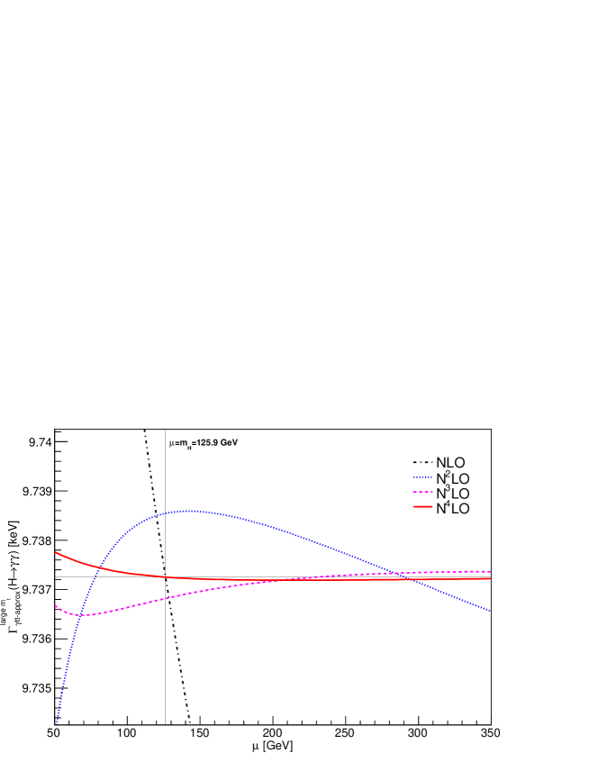
Figure 4: The dash-dotted, dotted, dashed and solid lines represent the inclusion of the two- (NLO), three- (N²LO) four- (N³LO) and five-loop (N⁴LO) contribution in QCD to the quantity $\Gamma^{\mbox{\tiny{large} }m_{t}}_{\mbox{\tiny{$\gamma tt$-approx}}}(H\to\gamma\gamma)$. The scale has been varied between 50 and 350 GeV which covers the complete mass scale range $m_{H}/2<\mu<2m_{t}$. The vertical line shows the location where the scale $\mu$ is equal to the mass of the Higgs boson $m_{H}$ and the horizontal line gives the value of $\Gamma^{\mbox{\tiny{large} }m_{t}}_{\mbox{\tiny{$\gamma tt$-approx}}}(H\to\gamma\gamma)$ for $\mu=m_{H}$ at N⁴LO accuracy.

The mass corrections and singlet contributions, which are not contained in Fig. 4, are known up to three-loop order. In the next step we include them too. The mass corrections decrease the decay width. For the numerical evaluation we use the following input parameters for the fine-structure constant $\alpha=1/137.035999074$ [58] and the strong coupling constant $\alpha_{s}(M_{Z})=0.1185$ [58], which we evolve to the Higgs-boson mass scale $\mu=m_{H}$. For the partial decay width including the QCD corrections we obtain for $m_{H}=125.9$ GeV [58]

$$\Gamma(H\to\gamma\gamma)=9.370_{\mbox{\tiny{1-loop}}}+0.168_{\mbox{\tiny{2-loop}}}+0.008_{\mbox{\tiny{3-loop}}}-0.002_{\mbox{\tiny{4-loop,$\gamma tt$-approx}}}+0.0004_{\mbox{\tiny{5-loop,$\gamma tt$-approx}}}\mbox{ keV}\,,$$

where each term corresponds to the next order in the perturbative expansion. The four- and five-loop orders contain only the contributions where the photons couple to a top quark in the heavy top-quark mass limit which is considered in this work. Their size can change once the complete result becomes available. Its calculation is beyond the scope of the present work.
We convert the top-quark mass to the on-shell scheme [63, 64, 65, 66, 67, 68] and include also the two-loop electroweak corrections of Refs. [11, 10]. For the Fermi-coupling constant we use $G_{F}=1.1663787\cdot 10^{-5}\mbox{ GeV}^{-2}$ [58] and obtain

$$\Gamma(H\to\gamma\gamma) = [9.384_{\mbox{\tiny{1-loop}}}+(0.159_{\mbox{\tiny{QCD}}}-0.150_{\mbox{\tiny{EW}}})_{\mbox{\tiny{2-loop}}}+0.004_{\mbox{\tiny{QCD, 3-loop}}}$$

$$-0.001_{\mbox{\tiny{QCD, 4-loop,$\gamma tt$-approx}}}+0.0006_{\mbox{\tiny{QCD, 5-loop,$\gamma tt$-approx}}}]\mbox{ keV}=9.396\mbox{ keV}\,.$$

The different terms corresponds to the one-loop, two-loop and three-loop contribution, where we have subdivided the two-loop term again into QCD and electroweak(EW) corrections. The partial decay width changes by about $\sim 0.13$ keV when the Higgs-boson mass is varied within its current uncertainty of $\pm 0.4$ GeV.

4 Summary and conclusion

The decoupling function $\zeta_{g\gamma}^{2}$ relates the $\overline{\mbox{MS}}$ renormalized fine-structure constant in the full theory with $n_{f}=n_{l}+1$ active quark flavors to the $\overline{\mbox{MS}}$ renormalized fine-structure constant in an effective theory with $n_{l}$ light active quark flavors. We have computed the complete decoupling function $\zeta_{g\gamma}^{2}$ at four-loop order in perturbative QCD for a general $SU(N_{c})$ color group as a new result. The decoupling function enters into the description of an effective Higgs-photon-photon coupling in the heavy top-quark mass limit. As an application of the calculation we have used the effective theory in order to determine the four-loop QCD corrections in the heavy top-quark mass limit to the decay amplitude $H\to\gamma\gamma$ for those contributions for which the photons couple directly to the top quark. The calculation of the amplitude agrees with a known, independent result in literature. In addition we also extended this calculation to five-loop order by using the anomalous dimensions in combination with the renormalization group equation of the vacuum polarization function. Finally we study the reduction of the scale dependence and perform a numerical evaluation of the partial decay width. Its dominant uncertainty arises from the error in the Higgs boson mass.

Acknowledgments
C.S. would like to thank Johann Kühn and Matthias Steinhauser for valuable discussions and comments on the manuscript.
The Feynman diagrams were drawn with the help of Axodraw[69] and Jaxodraw[70].

Appendix A The decoupling function up to three-loop order

The results for the decoupling function $\zeta_{ph}^{(k)}(\overline{m}_{t},\mu)$ of Eq. (8) up to three-loop order are known from Ref. [23] and read

$$\zeta_{ph}^{(0)}(\overline{m}_{t},\mu) = -Q_{t}^{2}\*{4\over 3}\*\ell_{\mu}\,,\qquad\qquad\zeta_{ph}^{(1)}(\overline{m}_{t},\mu)=-Q_{t}^{2}\*C_{F}\*\left({13\over 12}-\ell_{\mu}\right)\,,$$ (19)

$$\zeta_{ph}^{(2)}(\overline{m}_{t},\mu) = Q_{t}^{2}\*\Bigg{[}C_{F}^{2}\*\left(-{97\over 72}+{95\over 48}\*\zeta_{3}-{9\over 8}\*\ell_{\mu}\right)+C_{A}\*C_{F}\*\left({5021\over 2592}-{223\over 96}\*\zeta_{3}+{7\over 9}\*\ell_{\mu}+{11\over 24}\*\ell_{\mu}^{2}\right)$$ (20)

$$- n_{l}\*C_{F}\*T_{F}\*\left({361\over 648}-{\ell_{\mu}\over 9}+{\ell_{\mu}^{2}\over 6}\right)+n_{h}\*C_{F}\*T_{F}\*\left({103\over 324}-{7\over 16}\*\zeta_{3}+{\ell_{\mu}\over 9}-{\ell_{\mu}^{2}\over 6}\right)\Bigg{]}$$

$$- \sum_{i=1}^{n_{l}}Q_{q_{i}}^{2}\*n_{h}\*C_{F}\*T_{F}\*\left({295\over 648}-{11\over 36}\*\ell_{\mu}+{\ell_{\mu}^{2}\over 6}\right)\,.$$

The symbols which appear in Eqs. (19) and (20) are defined in Section 3.

Appendix B Fermionic amplitude in the heavy top-quark mass limit at two- and three-loop order

For completeness we give here the result for the fermionic amplitude at two- and three-loop order in the heavy top-quark mass limit

$$A^{(1)} = -{3\over 4}\*C_{F}\,,$$ (21)

$$A^{(2)} = {27\over 32}\*C_{F}^{2}-C_{F}\*\left[C_{A}\*\left({7\over 12}+{11\over 16}\*\ell_{\mu}\right)+n_{h}\*T_{F}\*\left({13\over 48}-{\ell_{\mu}\over 4}\right)+n_{l}\*T_{F}\*\left({1\over 12}-{\ell_{\mu}\over 4}\right)\right]$$ (22)

$$+ \mbox{si}\,\*C_{F}\*T_{F}\*\left[n_{h}\*{3\over 16}+Q_{t}^{-2}\*\sum_{i=1}^{n_{l}}Q_{q_{i}}^{2}\*\left(\zeta_{3}-{13\over 8}+{1\over 4}\*\ln\left(-{m_{h}^{2}\over\overline{m}_{t}^{2}}\right)\right)\right]\,,$$

where we have taken the last terms, which are proportional to $Q_{q_{i}}^{2}$, from Ref. [22]. The symbols which arise in Eqs. (21) and (22) are again defined in Section 3.

References

- [1] CMS Collaboration Collaboration, S. Chatrchyan et al., Observation of a new boson at a mass of 125 GeV with the CMS experiment at the LHC, Phys.Lett. B716 (2012) 30–61, arXiv:1207.7235 [hep-ex].
- [2] ATLAS Collaboration Collaboration, G. Aad et al., Observation of a new particle in the search for the Standard Model Higgs boson with the ATLAS detector at the LHC, Phys.Lett. B716 (2012) 1–29, arXiv:1207.7214 [hep-ex].
- [3] J. R. Ellis, M. K. Gaillard, and D. V. Nanopoulos, A Phenomenological Profile of the Higgs Boson, Nucl.Phys. B106 (1976) 292.
- [4] M. A. Shifman, A. Vainshtein, M. Voloshin, and V. I. Zakharov, Low-Energy Theorems for Higgs Boson Couplings to Photons, Sov.J.Nucl.Phys. 30 (1979) 711–716.
- [5] A. Vainshtein, V. I. Zakharov, and M. A. Shifman, Higgs Particles, Sov.Phys.Usp. 23 (1980) 429–449.
- [6] B. A. Kniehl and M. Spira, Low-energy theorems in Higgs physics, Z.Phys. C69 (1995) 77–88, arXiv:hep-ph/9505225 [hep-ph].
- [7] U. Aglietti, R. Bonciani, G. Degrassi, and A. Vicini, Two loop light fermion contribution to Higgs production and decays, Phys.Lett. B595 (2004) 432–441, arXiv:hep-ph/0404071 [hep-ph].
- [8] F. Fugel, B. A. Kniehl, and M. Steinhauser, Two loop electroweak correction of to the Higgs-boson decay into photons, Nucl.Phys. B702 (2004) 333–345, arXiv:hep-ph/0405232 [hep-ph].
- [9] G. Degrassi and F. Maltoni, Two-loop electroweak corrections to the Higgs-boson decay , Nucl.Phys. B724 (2005) 183–196, arXiv:hep-ph/0504137 [hep-ph].
- [10] G. Passarino, C. Sturm, and S. Uccirati, Complete Two-Loop Corrections to , Phys.Lett. B655 (2007) 298–306, arXiv:0707.1401 [hep-ph].
- [11] S. Actis, G. Passarino, C. Sturm, and S. Uccirati, NNLO Computational Techniques: The Cases and , Nucl.Phys. B811 (2009) 182–273, arXiv:0809.3667 [hep-ph].
- [12] H.-Q. Zheng and D.-D. Wu, First order QCD corrections to the decay of the Higgs boson into two photons, Phys.Rev. D42 (1990) 3760–3763.
- [13] S. Dawson and R. Kauffman, QCD corrections to , Phys.Rev. D47 (1993) 1264–1267.
- [14] A. Djouadi, M. Spira, J. van der Bij, and P. Zerwas, QCD corrections to gamma gamma decays of Higgs particles in the intermediate mass range, Phys.Lett. B257 (1991) 187–190.
- [15] K. Melnikov and O. I. Yakovlev, Higgs two photon decay: QCD radiative correction, Phys.Lett. B312 (1993) 179–183, arXiv:hep-ph/9302281 [hep-ph].
- [16] M. Inoue, R. Najima, T. Oka, and J. Saito, QCD corrections to two photon decay of the Higgs boson and its reverse process, Mod.Phys.Lett. A9 (1994) 1189–1194.
- [17] M. Spira, A. Djouadi, D. Graudenz, and P. Zerwas, Higgs boson production at the LHC, Nucl.Phys. B453 (1995) 17–82, arXiv:hep-ph/9504378 [hep-ph].
- [18] J. Fleischer, O. Tarasov, and V. Tarasov, Analytical result for the two loop QCD correction to the decay , Phys.Lett. B584 (2004) 294–297, arXiv:hep-ph/0401090 [hep-ph].
- [19] R. Harlander and P. Kant, Higgs production and decay: Analytic results at next-to-leading order QCD, JHEP 0512 (2005) 015, arXiv:hep-ph/0509189 [hep-ph].
- [20] U. Aglietti, R. Bonciani, G. Degrassi, and A. Vicini, Analytic Results for Virtual QCD Corrections to Higgs Production and Decay, JHEP 0701 (2007) 021, arXiv:hep-ph/0611266 [hep-ph].
- [21] M. Steinhauser, Corrections of to the decay of an intermediate mass Higgs boson into two photons, arXiv:hep-ph/9612395 [hep-ph].
- [22] P. Maierhöfer and P. Marquard, Complete three-loop QCD corrections to the decay , Phys.Lett. B721 (2013) 131–135, arXiv:1212.6233 [hep-ph].
- [23] K. Chetyrkin, B. A. Kniehl, and M. Steinhauser, Decoupling relations to and their connection to low-energy theorems, Nucl.Phys. B510 (1998) 61–87, arXiv:hep-ph/9708255 [hep-ph].
- [24] P. Baikov, K. Chetyrkin, J. Kühn, and J. Rittinger, Vector correlator in massless QCD at order and the QED -function at five loop, JHEP 1207 (2012) 017, arXiv:1206.1284 [hep-ph].
- [25] K. Chetyrkin, Quark mass anomalous dimension to , Phys.Lett. B404 (1997) 161–165, arXiv:hep-ph/9703278 [hep-ph].
- [26] J. Vermaseren, S. Larin, and T. van Ritbergen, The four loop quark mass anomalous dimension and the invariant quark mass, Phys.Lett. B405 (1997) 327–333, arXiv:hep-ph/9703284 [hep-ph].
- [27] T. van Ritbergen, J. Vermaseren, and S. Larin, The Four loop beta function in quantum chromodynamics, Phys.Lett. B400 (1997) 379–384, arXiv:hep-ph/9701390 [hep-ph].
- [28] M. Czakon, The Four-loop QCD beta-function and anomalous dimensions, Nucl.Phys. B710 (2005) 485–498, arXiv:hep-ph/0411261 [hep-ph].
- [29] S. Gorishnii, A. Kataev, and S. Larin, The corrections to and in QCD, Phys.Lett. B259 (1991) 144–150.
- [30] K. Chetyrkin, Corrections of order to (had) in pQCD with light gluinos, Phys.Lett. B391 (1997) 402–412, arXiv:hep-ph/9608480 [hep-ph].
- [31] K. Chetyrkin, J. H. Kühn, and M. Steinhauser, Three loop polarization function and corrections to the production of heavy quarks, Nucl.Phys. B482 (1996) 213–240, arXiv:hep-ph/9606230 [hep-ph].
- [32] K. Chetyrkin, J. H. Kühn, P. Mastrolia, and C. Sturm, Heavy-quark vacuum polarization: First two moments of the contribution, Eur.Phys.J. C40 (2005) 361–366, arXiv:hep-ph/0412055 [hep-ph].
- [33] K. Chetyrkin, J. H. Kühn, and C. Sturm, Four-loop moments of the heavy quark vacuum polarization function in perturbative QCD, Eur.Phys.J. C48 (2006) 107–110, arXiv:hep-ph/0604234 [hep-ph].
- [34] P. Nogueira, Automatic Feynman graph generation, J.Comput.Phys. 105 (1993) 279–289.
- [35] T. Seidensticker, Automatic application of successive asymptotic expansions of Feynman diagrams, arXiv:hep-ph/9905298 [hep-ph].
- [36] R. Harlander, T. Seidensticker, and M. Steinhauser, Complete corrections of Order to the decay of the Z boson into bottom quarks, Phys.Lett. B426 (1998) 125–132, arXiv:hep-ph/9712228 [hep-ph].
- [37] J. Vermaseren, New features of FORM, arXiv:math-ph/0010025 [math-ph].
- [38] J. Vermaseren, Tuning FORM with large calculations, Nucl.Phys.Proc.Suppl. 116 (2003) 343–347, arXiv:hep-ph/0211297 [hep-ph].
- [39] M. Tentyukov and J. Vermaseren, Extension of the functionality of the symbolic program FORM by external software, Comput.Phys.Commun. 176 (2007) 385–405, arXiv:cs/0604052 [cs-sc].
- [40] K. Chetyrkin and F. Tkachov, Integration by Parts: The Algorithm to Calculate beta Functions in 4 Loops, Nucl.Phys. B192 (1981) 159–204.
- [41] S. Laporta and E. Remiddi, The Analytical value of the electron (g-2) at order in QED, Phys.Lett. B379 (1996) 283–291, arXiv:hep-ph/9602417 [hep-ph].
- [42] S. Laporta, High precision calculation of multiloop Feynman integrals by difference equations, Int.J.Mod.Phys. A15 (2000) 5087–5159, arXiv:hep-ph/0102033 [hep-ph].
- [43] R. H. Lewis, Fermat User Guide, http://home.bway.net/lewis/.
- [44] Y. Schröder and A. Vuorinen, High-precision epsilon expansions of single-mass-scale four-loop vacuum bubbles, JHEP 0506 (2005) 051, arXiv:hep-ph/0503209 [hep-ph].
- [45] K. Chetyrkin, M. Faisst, C. Sturm, and M. Tentyukov, epsilon-finite basis of master integrals for the integration-by-parts method, Nucl.Phys. B742 (2006) 208–229, arXiv:hep-ph/0601165 [hep-ph].
- [46] D. J. Broadhurst, Three loop on-shell charge renormalization without integration: Lambda-MS (QED) to four loops, Z.Phys. C54 (1992) 599–606.
- [47] Y. Schröder and M. Steinhauser, Four-loop singlet contribution to the rho parameter, Phys.Lett. B622 (2005) 124–130, arXiv:hep-ph/0504055 [hep-ph].
- [48] D. J. Broadhurst, On the enumeration of irreducible k fold Euler sums and their roles in knot theory and field theory, arXiv:hep-th/9604128 [hep-th].
- [49] S. Laporta, High precision epsilon expansions of massive four loop vacuum bubbles, Phys.Lett. B549 (2002) 115–122, arXiv:hep-ph/0210336 [hep-ph].
- [50] B. A. Kniehl and A. V. Kotikov, Calculating four-loop tadpoles with one non-zero mass, Phys.Lett. B638 (2006) 531–537, arXiv:hep-ph/0508238 [hep-ph].
- [51] B. A. Kniehl and A. V. Kotikov, Heavy-quark QCD vacuum polarisation function: Analytical results at four loops, Phys.Lett. B642 (2006) 68–71, arXiv:hep-ph/0607201 [hep-ph].
- [52] B. Kniehl, A. Kotikov, A. Onishchenko, and O. Veretin, Strong-coupling constant with flavor thresholds at five loops in the anti-MS scheme, Phys.Rev.Lett. 97 (2006) 042001, arXiv:hep-ph/0607202 [hep-ph].
- [53] K. Chetyrkin, J. H. Kühn, and C. Sturm, QCD decoupling at four loops, Nucl.Phys. B744 (2006) 121–135, arXiv:hep-ph/0512060 [hep-ph].
- [54] Y. Schröder and M. Steinhauser, Four-loop decoupling relations for the strong coupling, JHEP 0601 (2006) 051, arXiv:hep-ph/0512058 [hep-ph].
- [55] A. Grozin, P. Marquard, J. Piclum, and M. Steinhauser, Three-Loop Chromomagnetic Interaction in HQET, Nucl.Phys. B789 (2008) 277–293, arXiv:0707.1388 [hep-ph].
- [56] A. Grozin, M. Höschele, J. Hoff, and M. Steinhauser, Simultaneous Decoupling of Bottom and Charm Quarks, PoS LL2012 (2012) 032, arXiv:1205.6001 [hep-ph].
- [57] P. Marquard, L. Mihaila, J. Piclum, and M. Steinhauser, Relation between the pole and the minimally subtracted mass in dimensional regularization and dimensional reduction to three-loop order, Nucl.Phys. B773 (2007) 1–18, arXiv:hep-ph/0702185 [hep-ph].
- [58] Particle Data Group Collaboration, J. Beringer et al., Review of Particle Physics (RPP), Phys.Rev. D86 (2012) 010001.
- [59] K. Chetyrkin, J. H. Kühn, and M. Steinhauser, RunDec: A Mathematica package for running and decoupling of the strong coupling and quark masses, Comput.Phys.Commun. 133 (2000) 43–65, arXiv:hep-ph/0004189 [hep-ph].
- [60] M. Steinhauser, MATAD: A Program package for the computation of MAssive TADpoles, Comput.Phys.Commun. 134 (2001) 335–364, arXiv:hep-ph/0009029 [hep-ph].
- [61] S. Gorishnii, S. Larin, L. Surguladze, and F. Tkachov, Mincer: Program for Multiloop Calculations in Quantum Field Theory for the Schoonschip System, Comput.Phys.Commun. 55 (1989) 381–408.
- [62] S. Larin, F. Tkachov, and J. Vermaseren, The FORM version of MINCER, NIKHEF-H-91-18.
- [63] R. Tarrach, The Pole Mass in Perturbative QCD, Nucl. Phys. B183 (1981) 384.
- [64] N. Gray, D. J. Broadhurst, W. Grafe, and K. Schilcher, Three loop relation of quark (modified) MS and pole masses, Z.Phys. C48 (1990) 673–680.
- [65] K. Chetyrkin and M. Steinhauser, Short distance mass of a heavy quark at order , Phys.Rev.Lett. 83 (1999) 4001–4004, arXiv:hep-ph/9907509 [hep-ph].
- [66] K. Chetyrkin and M. Steinhauser, The Relation between the and the on-shell quark mass at order , Nucl.Phys. B573 (2000) 617–651, arXiv:hep-ph/9911434 [hep-ph].
- [67] K. Melnikov and T. van Ritbergen, The Three loop on-shell renormalization of QCD and QED, Nucl.Phys. B591 (2000) 515–546, arXiv:hep-ph/0005131 [hep-ph].
- [68] K. Melnikov and T. v. Ritbergen, The Three loop relation between the and the pole quark masses, Phys.Lett. B482 (2000) 99–108, arXiv:hep-ph/9912391 [hep-ph].
- [69] J. Vermaseren, Axodraw, Comput.Phys.Commun. 83 (1994) 45–58.
- [70] D. Binosi and L. Theussl, JaxoDraw: A Graphical user interface for drawing Feynman diagrams, Comput.Phys.Commun. 161 (2004) 76–86, arXiv:hep-ph/0309015 [hep-ph].