High-dimensional Lifshitz-type spacetimes, universal horizons and black holes in Hořava-Lifshitz gravity
Kai Lin a,blk314159@hotmail.comFu-Wen Shu cshufuwen@ncu.edu.cnAnzhong Wang a,d111Corresponding authoranzhong˙wang@baylor.eduQiang Wu awuq@zjut.edu.cna Institute for Advanced Physics Mathematics,
Zhejiang University of
Technology, Hangzhou 310032, China
b Instituto de Física, Universidade de São Paulo, CP 66318, 05315-970, São Paulo, Brazil
c Center for Relativistic Astrophysics and High Energy Physics, Nanchang University, Nanchang 330031, China
d GCAP-CASPER, Physics Department, Baylor University, Waco, TX 76798-7316, USA
Abstract
In this paper, we present all -dimensional static diagonal vacuum solutions of the non-projectable Hořava-Lifshitz
gravity in the IR limit, and show that they give rise to very rich Lifshitz-type structures, depending on the choice of the free parameters
of the solutions. These include the Lifshitz spacetimes with or without hyperscaling violation, Lifshitz solitons, and black holes.
Remarkably, even the theory breaks explicitly the Lorentz symmetry and allows generically instantaneous propagations, universal
horizons still exist, which serve as one-way membranes for signals with any large velocities. In particular, particles even with
infinitely large velocities would just move around on these boundaries and cannot escape to infinity. Another remarkable feature
appearing in the Lifshitz-type spacetimes is that the dynamical exponent can take its values only in the ranges for
and for , due to the stability and ghost-free conditions of the theory.
pacs:
04.60.-m; 98.80.Cq; 98.80.-k; 98.80.Bp
I Introduction
Lifshitz space-time has been extensively studied in the content of non-relativistic gauge/gravity duality Mann ; HKW , after the seminal work of
KLM , which argued that nonrelativistic quantum field theories (QFTs) that describe multicritical points in certain magnetic materials and liquid crystals Sachdev
may be dual to certain nonrelativistic gravitational theories in such a space-time background.
One of the remarkable feature of the Lifshitz space-time is its anisotropic scaling between space and time,
(1.1)
on a hypersurface Constant, on which the nonrelativistic QFTs live, where denotes the dynamical critical exponent, and in the relativistic scaling we have
. denote the spatial coordinates tangential to the surfaces Constant.
It is interesting to note that the anisotropic scaling (1.1) can be realized in two different levels. In Level one, the underlying theory itself is still relativistic-scaling invariant,
but the space-time has the anisotropic scaling. This was precisely the case studied in KLM ; Mann , where the theories of gravity is still of general covariance, but
the metric of the space-time has the above anisotropic scaling. This is possible only when some matter fields are introduced to create a preferred direction, so that the
anisotropic scaling (1.1) can be realized. In KLM , this was done by two p-form gauge fields with , and was soon generalized to different cases Mann .
In Level two, not only the space-time has the above anisotropic scaling, but also the theory itself. In fact, starting with the anisotropic scaling (1.1), Hořava
recently constructed a theory of quantum gravity at a Lifshitz fixed point, the so-called Hořava-Lifshitz (HL) theory Horava ,
which is power-counting renormalizable, and lately has attracted lots of attention, due to its remarkable features when applied to cosmology and
astrophysics reviews . Power-counting renomalizability requires , where denotes the number of spatial dimensions of the theory.
Since the anisotropic scaling (1.1) is built in by construction in the HL gravity, it is natural to expect that the HL gravity provides a minimal holographic dual for
non-relativistic Lifshitz-type field theories with the anisotropic scaling. Indeed, this was first showed in GHMT
that the Lifshitz spacetime,
(1.2)
is a vacuum solution of the HL gravity in (2+1) dimensions, and that the full structure of the anisotropic Weyl anomaly can be reproduced in dual field theories,
while its minimal relativistic gravity counterpart yields only one of two independent central charges in the anomaly.
Recently, we studied the HL gravity in (2+1) dimensions in detail SLWW , and found further evidence to support the above speculations. In particular, we found all
the static (diagonal) solutions of the HL gravity in (2+1) dimensions, and showed that they give rise to very rich space-time structures: the corresponding spacetimes
can represent the generalized Banados, Teitelboim and Zanelli (BTZ) black holes BTZ , the Lifshitz space-times, or Lifshitz solitons LSolitons , in which the spacetimes are free of any kind
of space-time singularities, depending on the choices of the free parameters of the solutions. Some space-times are not complete, and extensions beyond certain horizons
are needed. In addition, it was shown recently that the Lifshitz space-time (1.2) is not only a solution of the HL gravity in the IR, but also a solution of the full theory, that is,
even high-order operators are all included WYTWDC . The only effects of these high-order operators are to shift from one value to another, as longer as
the spacetime itself is concerned.
In this paper, we shall generalize our above studies to any dimensions, and obtain all the static (diagonal) solutions of the vacuum HL gravity explicitly.
With these exact vacuum solutions,we believe that the studies of the non-relativistic Lifshitz-type gauge/gravity duality will be simplified considerably, as
so far most of such studies are numerical Mann ; GR10 ; LSolitons ; LBHs ; OTU . After studying each of
these solutions in detail, we find that, similar to the (2+1) case, Lifshitz space-times and solitons can be all found in
these solutions. Remarkably, the Lifshitz space-times with hyperscaling violation GR10 ; OTU ,
(1.3)
can be also realized in the HL gravity as a vacuum solutions of the theory.
Moreover, some of the solutions to be presented in this paper also represent black holes, although the HL gravity explicitly breaks Lorentz symmetry and allows
in principle propagations with any large velocities Horava ; reviews . This follows the recent discovery of the existence of the universal horizons in the khrononmetric
theory of gravity BS11 , in which the khronon naturally defines a timelike foliations, parametrized by Constant. Among
these leaves, there may exist a surface at which diverges, while physically nothing
singular happens there, including the metric and the space-time. Given that defines an absolute time, any object crossing this surface from the interior would necessarily also move back in
absolute time, which is something forbidden by the definition of the causality in the theory. Thus, even particles with superluminal velocities cannot penetrate this surface, once they are
trapped inside it. In particular, particles even with infinitely large velocities would just move around on these
boundaries and cannot escape to infinity. For more details, we refer readers to BS11 ; UHs ; LACW .
The rest of the paper is organized as follows: In Section II, we give a brief introduction
to the (d+2)-dimensional HL gravity without the projectablity condition, while in Section III we first write down the corresponding field equations for static vacuum spacetimes,
and then solve them for particular cases. In Section IV, we first obtain all the rest of the static (diagonal) vacuum (d+2)-dimensional solutions of the HL theory, and then study
each of such solutions in detail. In Section V, following LACW ; LGSW we study the black hole structures of solutions presented in Section III, and show explicitly that universal horizons
exist in some of these solutions. Finally, in Section VI we present our main conclusions and provide some discussing remarks.
II Non-projectable HL theory in dimensions
In this paper, we shall take the Arnowitt-Deser-Misner (ADM) variables ADM ,
(2.1)
as the fundamental ones, which are all functions of both and , as in this paper we shall work in the version of the HL
gravity without the projectability condition Horava ; reviews . Then, the general action of the HL theory
in (d+2)-dimensions is given by
(2.2)
where , , and
(2.3)
Here is a dimensionless
coupling constant, and denotes the covariant derivative with respect to . is the Lagrangian of matter
fields. The potential is constructed from and , and formally can be written in the form,
(2.4)
where denotes the part that includes
all higher-order operators ZWWS . Power-counting renormalizability condition requires Horava ; reviews . denotes the Ricci tensor made of , and
(2.5)
In the infrared (IR) limit, the higher-order operators are suppressed by , so we can safely
set them to zero,
(2.6)
where and denotes the order of the operator. In this paper, we shall consider only the IR limit, so that
Eq.(2.6) is always true.
II.1 Field Equations in IR Limit
Variation of the action (2.2) with respect to the lapse
function yields the Hamiltonian constraint
(2.7)
where
(2.8)
Variation with respect to the shift vector yields the momentum constraint
(2.9)
where
(2.10)
The dynamical equations are obtained by varying the action with respect to , and are given by
(2.11)
where
(2.12)
with .
In addition, the matter components satisfy the conservation laws of energy and momentum,
(2.13)
(2.14)
II.2 Stability and Ghost-free Conditions
When , the above HL theory admits the Minkowski space-time
(2.15)
as a solution of the theory. Then, its linear perturbations reveals that the theory has two modes GHMT , one represents the spin-2 massless
gravitons with a dispersion relation,
(2.16)
and the other represents the scalar mode with
(2.17)
The stability conditions of these modes requires
(2.18)
for any given .
On the other hand, the kinetic term of the scalar mode is proportional to GHMT , so the
ghost-free condition requires
(2.19)
which is equivalent to
(2.20)
Then, Eq.(2.18) implies that 222It is interesting to note that in (2+1)-dimensions, the spin-2 gravitons do not exist, so the
coupling constant is free, while is required to be negative, SLWW .
(2.21)
III Static vacuum solutions
In this paper, we consider static spacetimes given by,
(3.1)
in the coordinates , where . Note that in SLWW , the case was studied in detail.
So, in this paper we shall consider only the case where
.
Then, the dimensional Ricci scalar
of the leaves Constant is given by
(3.2)
On the other hand, since and that the spacetimes are static, so we must have . Then, the momentum
constraint (2.9) is satisfied identically. The Hamiltonian constraint (2.7) and the -component of the dynamical equations (II.1) are non-trivial, while
the -component of the dynamical equations can be
derived from the Hamiltonian constraint and the component. Therefore, similar to the (2+1)-dimensional case, there are only two independent
equations for two unknowns, and , which can be cast in the forms,
Then, from the stability conditions (2.21) we find that
(3.8)
where the equality holds only when , which is possible when , as can be seen from Eq.(2.17).
Inserting the above expression into Eq.(III), we obtain a master
equation for ,
(3.9)
where , and
(3.10)
Note that Eq.(3.9) with sign can be always obtained from the one with sign, by simply replacing by .
Therefore, although defined by Eq.(III)
is non-negative, we shall take the region as a natural extension, so that
in the following we only need to consider the case with sign.
Therefore, once the master equation (3.9) is solved for , substituting it into Eq.(3.12) we can find . Then, in terms of , the metric takes the form,
(3.13)
In the rest of this section, we shall solve the above equations for some particular cases, and leave the one with to the next section.
III.1 Lifshitz Spacetime
A particular solution of Eq.(3.9) is . Then we obtain
(3.14)
where in terms of , the cosmological constant is given by,
(3.15)
with and being the integration constants. Then, the corresponding line element takes the form,
(3.16)
where , and
(3.17)
which is independent of the space-time dimensions. On the other hand, from the stability and ghost-free condition (2.21), it can be shown that
(3.18)
Note that the above holds only for . In particular, we have
(3.19)
This is a unexpected result, but seems to agree with some numerical solutions found in other theories of gravity Mann .
Rescaling the coordinates , without loss of generality, one can always set .
Then, we find that the corresponding curvature is
given by
(3.20)
which is a constant.
It is remarkable to note that when , is also a solution of Eq. (3.9). In this case we have the same
Lifshitz solution (3.16) but and now are given by,
(3.21)
III.2 Generalized BTZ Black Holes
When , we find that . Then, from the stability conditions (2.21) we can see that this is possible only when . Thus, we obtain
(3.22)
for which the metric takes the form,
where “+” (“-”) corresponds to (), and .
Since [cf. Eq.(2.21)], we find that, to have non-negative, we must require
(3.24)
For , the above is possible only when , for which, by rescaling and , the metric (III.2) can be cast in the form,
(3.25)
which is nothing but the -dimensional BTZ black holes BTZ with the black hole mass given by , where .
It should be noted that the original BTZ black hole was obtained in general relativity, for which we have .
Clearly, the above solutions are valid for any given . In this sense we refer these black holes to as the generalized BTZ black holes.
Note that when , we obtain . Then, substituting it into the expression for
we obtain . However, the condition (3.8) require . Therefore, in the current
case, cannot vanish.
On the other hand, when , from Eqs.(3.8) and (III), we find that this is possible only when
, which is not allowed by Eq.(3.8). Therefore, is also impossible in the current case.
Thus, in the rest of this paper, we only need to consider the case , which will be studied in the next
section.
IV Static Spacetimes for
The condition implies,
(4.1)
However, Eq.(3.8) further exclude the region . Therefore, in this section we need only to consider the case where
Since , as it can be seen from Eq.(IV.1), we find that only the root satisfies this condition.
On the other hand, from Eqs.(4.8) and (3.11) we find,
(4.25)
(4.26)
where
(4.27)
(b) , we have , and now . Thus we find that
(4.28)
are solutions to Eq. (4.20) in this region. This immediately leads to,
(4.29)
(4.30)
(c) , we have , implying . Then, we find that
are solutions to Eq. (4.20). We therefore obtain the same forms as region (b) for functions and
(4.32)
(4.33)
(d) , we have , implying . Then, we find that
are solutions to Eq. (4.20). We therefore obtain the functions and
(4.35)
(4.36)
IV.2
In this case, we find that . Then, we obtain
(4.37)
where and are two integration constants. Then, the corresponding metric takes the form
(4.38)
Clearly, to have positive, we must assume that
(4.39)
The corresponding Ricci scalar is given by
(4.40)
which remains finite at the hypersurface , and indicate that it might represent a horizon, where .
As , the metric takes the following
asymptotical form,
where , and
(4.42)
Rescaling and , the above metric can be cast in the form,
(4.43)
where
(4.44)
The metric (4.43) is nothing but the space-time with non-relativistic scaling and hyperscaling violation. It was first constructed in Einstien-Maxwell-dilaton theories GR10 ,
and recently has been extensively studied in OTU . Under the anisotropic scaling (1.1), it is not invariant but rather scaling as .
This kind of non-relativistic scaling is closely related to the existence of Fermi surfaces, in which the entanglement entropy is logarithmically proportional to the erea, .
IV.3
In this case, we have
(4.45)
Note that in the current case we have .
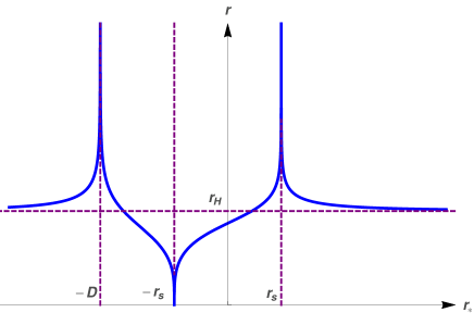
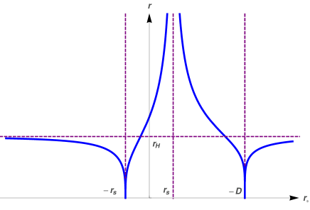
Fig. 2 shows the function vs , from which we can see that the region is mapped into the region or
. The region or is mapped into the one .
Figure 2: The function for and
, where in the present case. The spacetime is singular at .
Similar to the previous cases, let us consider the case with in detail, which corresponds to
(4.46)
Then, we find that
(4.47)
Following what we did for the previous cases, one can solve it for in the following four regions.
(a) . In this region, we have the following solution
Then, the functions and are given by
(4.48)
(4.49)
(b) . In this region, we have the following solution
Then, the functions and are given by
(4.50)
(4.51)
(c) . In this region, we have the following solution
Then, the functions and are given by
(4.52)
(4.53)
(d) . In this region, we have the following solution
To solve the above equation, we first write the above equation in the form,
(4.58)
which has the general solution,
(4.59)
Thus, we have
(4.60)
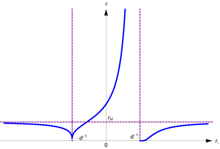
Fig. 3 shows the curve of vs . From the definition
of , on the other hand, we find that
(4.61)
which has the general solution,
(4.62)
Therefore, the corresponding metric takes the form,
(4.63)
where
(4.64)
where is given by Eq.(4.59). Then, the corresponding Ricci scalar is given by
(4.65)
from which it can be seen that the space-time is singular at . Then, the physical interpretation of the solutions
in the region is not clear. On the other hand, to have a complete space-time in
or , extensions beyond the hypersurfaces are needed.
Figure 3: The function for .
The space-time is singular at , as can be seen
from Eq.(4.65).
IV.5
In this case, we have
(4.66)
Similar to the last case, now but with .
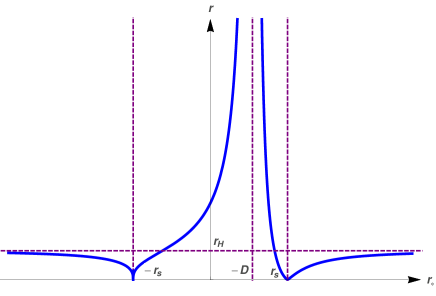
Fig. 4 shows the function vs , from which we can see that the region is mapped into the region or
. The region or is mapped into the one .
Figure 4: The function for
, where now . The spacetime is singular at ,
and asymptotically Lifshitz as .
Similar to the previous cases, let us consider the case with in detail, which corresponds to
(4.67)
Then, we find that
(4.68)
Following what we did for the previous cases, one can solve it for in the following four regions.
(a) . In this region, we have the following solution
(4.69)
where is defined as
(4.70)
Since ], we have for . The functions and are also given by
(4.71)
(4.72)
from which we can see that becomes unbounded at (or ). As shown above, this is a coordinate singularity.
To extend the above solution to the region , one may simply assume that Eq.(4.70) hold also for . In particular, setting
, we find that
(4.73)
where is defined by
(4.74)
The above expression represents an extension of the solution originally defined only for . Note that
as . Then, from Eq.(4.71) we find that
(4.75)
as . That is, the space-time is asymptotically approaching to a Lifshitz space-time with its dynamical exponent now given by
(b) . In this region, we have the following solution
(4.76)
Then, the functions and are given
by
(4.77)
(4.78)
(c) . In this region, we have the following solution
(d) . In this region, we have the following solution
(4.83)
where is defined by Eq.(4.70), so that . Then, the functions and are given by
(4.84)
(4.85)
Clearly, the metric becomes singular at . But this singularity is just a coordinate singularity and extension beyond this surface is needed.
Simply assuming that Eq.(4.70) holds also for will lead to to be a complex function of , and so are
the functions and . Therefore, this will not represent a desirable extension.
V Universal Horizons and Black Holes
Remarkably, studying the behavior of a khronon field in the fixed Schwarzschild black hole background,
(5.1)
where , Blas and Sibiryakov showed that a universal horizon exists
inside the Killing horizon.
But, in contrast to it, now the universal horizon is spacelike, and on which
the time-translation Killing vector becomes orthogonal to ,
(5.2)
where is the normal unit vector of the timelike foliations Constant,
(5.3)
with . Since is well-defined in the whole space-time, and remains timelike
from the asymptotical infinity () all the way down to the space-time singularity (),
Eq.(5.2) is possible only inside the Killing horizon, as only there becomes spacelike and can be
possibly orthogonal to .
The above definition of the universal horizons can be easily generalized to any theory that breaks Lorentz symmetry either in
the level of the action, such as the HL gravity studied in this paper, or spontaneously, such as
the khrononmetric theory BS11 , ghost condensation GC , Einstein-aether theory EA 333When the aether field is
hypersurface-orthoginal, ,
where denotes the covariant derivative with respect to the bulk metric , the
the Einstein-aether theory is equivalent to the khrononmetric theory, as
shown explicitly in Jacobson10 [See also Wang13 ; BS11 ]., and massive gravity mGR .
The idea is simply to consider the khronon field as a probe field that plays the same role as a Killing vector field for any given space-time LACW ; LGSW .
The equation that the khronon must satisfy in a given background can be obtained form the action LACW ; LGSW ,
(5.4)
where , and ’s are arbitrary constants 444Because of the hypersurface-orthogonal condition, only three of them are
independent LACW ; LGSW ; Jacobson10 . But, here we shall leave this possibility open. . Then,
the variation of with respect to yields,
(5.5)
where,
(5.6)
To solve Eq.(5.5) in terms of directly, it is very complicated usually, as high-order spatial derivatives of are often involved, and the equation is highly nonlinear.
So, often one divides the task into two steps: (i) One first solves it in terms of , so the corresponding equation becomes second-order, although it is still quite nonlinear.
(ii) Once is given, one can find by integrating out Eq.(5.3). However, as far as the universal horizon is concerned, Eq.(5.2) shows that
the second step is even not needed. Therefore, to find the location of the universal horizon now reduces first to solve Eq.(5.5) to obtain , subjected to the unit
and hypersurface-orthoginal conditions,
(5.7)
and then solve Eq.(5.2). Similar to the spherical case Jacobson10 , the four-velocity in the spacetimes,
(5.8)
is always hypersurface-orthoginal. Hence, the conditions given by Eq.(5.7) in the spacetimes of Eq.(5.8) simply reduces to , which can be written as
(5.9)
where .
In review of the above, one can see that solving the khronon equation (5.5) now reduces to solve it in terms of ,
subjected to the constraint (5.9). As mentioned above, it is a second-order differential equation in terms of . Therefore, to determine uniquely , two boundary
conditions are required, which can be BS11 ; LACW : (i) The khronon vector is
aligned asymptotically with the timelike Killing vector, .
(ii) The khronon field has a regular future sound horizon.
Even with all the above simplification, it is found still very difficult to solve khronon equation (5.5)
in the general case. But, when we find that Eq.(5.5) has a
simple solution , where is an integration
constant. Then, from Eq.(5.9) we can get , so finally we have,
(5.10)
where
(5.11)
Clearly, in order for the khronon field to be well-defined, we must assume
(5.12)
in the whole space-time, including the internal region of a Killing horizon, in which we have
. In addition, , as , as longer as remains positive. The latter is true for the case where spacetimes
are either asymptotically flat or anti-de Sitter. Moreover, for the choice , the khronon has an infinitely large speed LGSW . Then, by definition the universal horizon
coincides with the sound horizon of the spin-0 khronon mode. So, the regularity
of the khronon on the sound horizon now becomes the regularity on the universal horizon.
On the other hand,
from Eq.(5.2) we find that
(5.13)
at the universal horizons. Then, from the regular condition (5.12) we can see that the universal horizon located at must be also a minimum of . Therefore,
at the universal horizons we must have BBM ; LACW ; LGSW ,
(5.14)
which are equivalent to
(5.15)
(5.16)
The corresponding surface gravity is given by CLMV ,
(5.17)
For the solutions found in Section III, we can see that only the generalized BTZ solutions have Killing horizons, and possibly have also universal horizons.
For this class of solutions, we have
(5.18)
for which the condition requires . Applying the above formulas to this class of solutions, we find that universal horizons indeed exist, and
are given by,
(5.19)
In addition, we also have
(5.20)
where and denotes, respectively, the location of the Killing horizon and the corresponding surface gravity.
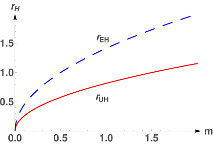
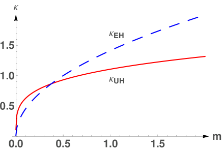
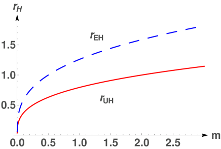
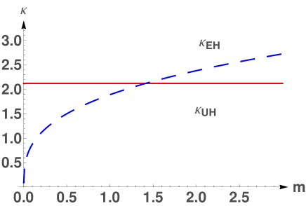
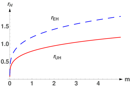
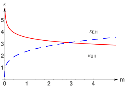
Figs. 5 - 7 show the locations of the universal and Killing horizons vs the mass parameter in spacetimes with , respectively.
In these figures, the corresponding surface gravities on the universal and Killing horizons are also given. From them we can see that the
universal horizons are always inside the Killing horizons, as they should be [cf. the explanations given above]. On the other hand, when , the surface gravity on the
universal horizon is always granter than the surface gravity on the Killing horizon, where is defined by . But, for
, the opposite, i.e., , always happens. It is interesting to note that is independent of in the case .
Figure 5: The locations of the universal horizon and
Killing (event) horizon and the corresponding surface gravities and on the universal and killing (event) horizon, respectively, for
the solutions and .
Figure 6: The locations of the universal horizon and
Killing (event) horizon and the corresponding surface gravities and on the universal and killing (event) horizon, respectively, for
the solutions and .
Figure 7: The locations of the universal horizon and
Killing (event) horizon and the corresponding surface gravities and on the universal and killing (event) horizon, respectively, for
the solutions and .
VI Conclusions
In this paper, we have generalized our previous studies of Lifshitz-type spacetimes in the HL gravity from -dimensions SLWW to
-dimensions with , and found explicitly all the static diagonal vacuum solutions of the HL gravity without the projectability condition in the IR limit.
After studying each of these solutions in detail (in Sections III - V), we have found that these solutions have very rich physics, and can give rise to
almost all the structures of Lifshitz-type spacetimes found so far in other theories of gravity, including the Lifshitz spacetimes KLM ; Mann ,
generalized BTZ black holes BTZ , Lifshitz solitons LSolitons , and Lifshitz spacetimes
with hyperscaling violation GR10 ; OTU , all depending on the free parameters of the solutions. Some solutions represent geodesically incomplete
spacetimes, and extensions beyond certain horizons are needed. After the extension, it is expected that some of them may represent Lifshitz-type black holes
LBHs .
A unexpected feature is that the dynamical exponent in all the solutions can take values in the range for and for ,
because of the stability and ghost-free conditions given by Eqs.(2.20) and (2.21). Note that in (2+1)-dimensions the range of takes its values from the range
, as shown explicitly in SLWW . A up bound of in high-dimensional spacetimes was also found in some numerical solutions in Mann ; LSolitons ; LBHs .
Another remarkable feature is the existence of black holes in the theory, considering the fact that the Lorentz symmetry is broken in this theory and propagations with instantaneous
interactions exist. Similar to the Einstein-aether theory BS11 ; UHs , there exist regions that are causally disconnected from infinity by surfaces of finite areas — the universal
horizons. Particles even with infinitely large velocity would just move around on these horizons and cannot escape to infinity. Such charged black holes have been also found recently
in the HL gravity LACW . In addition, using the tunneling approach for Hawking radiation, it was shown that the universal horizon indeed radiates thermally, and a thermodynamical interpretation
of the first law is possible BBM .
Yet, only the surface gravity defined by Eq.(5.17) is adopted, which was obtained after the nonrelativistic nature of the particle dynamics
was taken properly into account CLMV , can the standard relation between the Hawking temperature and the surface
gravity hold for the particular solutions of the Einstein-aether theory studied in BBM . The covariant form of the surface gravity Eq.(5.17) was further confirmed
by considering the peeling behavior of the khronon at the universal horizons for the
three well-known classical solutions, the Schwarzschild, Schwarzschild anti-de Sitter, and Reissner-Nordström LGSW . It is not difficult to show that the black hole solutions presented in
our current paper satisfy the first law of thermodynamics at the universal horizons, and the standard relation holds with the the surface gravity defined by Eq.(5.17).
Note that black holes defined by anisotropic horizons in the HL gravity were proposed recently in HMTb , and it would be very interesting to study space-time structures of the
solutions presented in this paper in terms of these anisotropic horizons, not to mention the infinitely red-shifted horizons, proposed recently in EHs .
With these exact vacuum solutions, it is expected that the studies of the non-relativistic Lifshitz-type gauge/gravity duality will be simplified considerably, and we
wish to return to these issues soon. The stability of these structures is another important issue that must be addressed.
Acknowledgements
This work is supported in part by DOE Grant, DE-FG02-10ER41692 (A.W.);
Ciência Sem Fronteiras, No. 004/2013 - DRI/CAPES (A.W.);
NSFC No. 11375153 (A.W.), No. 11173021 (A.W.),
No. 11005165 (F.W.S.); 555 Talent Project of Jiangxi Province, China (F.W.S.);
NSFC No. 11178018 (K.L.), No. 11375279 (K.L.);
FAPESP No. 2012/08934-0 (K.L.);
and NSFC No. 11205133 (Q.W.).
References
(1) K. Balasubramanian and K. Narayan, J. High Energy Phys. 08, 014 (2010);
A. Donos and J.P. Gauntlett, inid., 12, 002 (2010);
R. Gregory, S.L. Parameswaran, G. Tasinato, and I. Zavala,
inid., 1012 (2010) 047;
K. Copsey and R. Mann, inid., 03, 039 (2011);
P. Dey, and S. Roy, ibid., 11, 113 (2013);
G.T. Horowitz and W. Way, Phys. Rev. D85, 046008 (2013);
and references therein.
(2) B. Bao, X. Dong, S. Harrison, and E. Silverstein, Phys. Rev. D86, 106008 (2012);
T. Biswas, E. Gerwick, T. Koivisto, A. Mazumdar, Phys. Rev. Lett. 108, 031101 (2012);
S. Harrison, S. Kachru, and H. Wang, arXiv:1202.6635;
G. Knodel and J. Liu, arXiv:1305.3279;
S. Kachru, N. Kundu, A. Saha, R. Samanta, and S.P. Trivedi, arXiv:1310.5740.
(3) S. Kachru, X. Liu, and M. Mulligan, Phys. Rev. D78, 106005 (2008).
(4) S. A. Hartnoll, Class. Quant. Grav. 26, 224002 (2009);
J. McGreevy, Adv. High Energy Phys. 2010, 723105 (2010);
G.T. Horowitz, arXiv:1002.1722; S. Sachdev, Annu. Rev. Condens. Matter Phys. 3, 9 (2012).
(5) P. Hořava, Phys. Rev. D79, 084008 (2009) [arXiv:0901.3775].
(6) D. Blas, O. Pujolas, and S. Sibiryakov, J J. High Energy Phys. 1104, 018 (2011);
S. Mukohyama, Class. Quantum Grav. 27, 223101 (2010);
P. Hořava, Class. Quantum Grav. 28, 114012 (2011); T. Clifton, P.G. Ferreira, A. Padilla, and C. Skordis, Phys. Rept. 513, 1 (2012).
(7) T. Griffin, P. Hořava, and C. Melby-Thompson, Phys. Rev. Lett. 110, 081602 (2013).
(8) F.-W. Shu, K. Lin, A. Wang, and Q. Wu, J. High Energy Phys. 04 (2014) 056.
(9) M. Banados, C. Teitelboim, and J. Zanelli, Phys. Rev. Lett. 69, 1849 (1992).
(10) U. H. Danielsson and L. Thorlacius, J. High Energy Phys. 03, 070 (2009);
R. Mann, L. Pegoraro, and M. Oltean, Phys. Rev. D84, 124047 (2011);
H.A. Gonzalez, D. Tempo, and R. Troncoso, JHEP 11, 066 (2011).
(11) X. Wang, J. Yang, M. Tian, A. Wang, Y.-B. Deng, and G. Cleaver, arXiv:1407.1194.
(12) R.B. Mann, J. High Energy Phys. 06, 075 (2009);
G. Bertoldi, B. Burrington, and A. Peet, Phys. Rev. D80, 126003 (2009);
K. Balasubramanian, and J. McGreevy, Phys. Rev. D80 (2009) 104039 ;
E. Ayon-Beato, A. Garbarz, G. Giribet, M. Hassaine, Phys. Rev. D80 (2009) 104029;
R.-G. Cai, Y. Liu, Y.-W. Sun, JHEP0910 (2009) 080;
M.R. Setare and D. Momeni, Inter. J. Mod. Phys. D19, 2079 (2010);
Y.S. Myung, Phys. Lett. B690, 534 (2010);
D.-W. Pang, JHEP1001 (2010) 116;
E. Ayon-Beato, A. Garbarz, G. Giribet, M. Hassaine, JHEP 1004 (2010) 030;
M. H. Dehghani and R. B. Mann, J. High Energy Phys. 07, 019 (2010);
M.H. Dehghani, R.B. Mann, and R. Pourhasan, Phys. Rev. D84, 046002 (2011);
W. G. Brenna, M. H. Dehghani, and R. B. Mann, Phys. Rev. D84, 024012 (2011);
J. Matulich and R. Troncoso, J. High Energy Phys. 10 118 (2011).
I. Amado and A.F. Faedo, JHEP 1107, 004 (2011);
L. Barclay, R. Gregory, S. Parameswaran, G. Tasinato, JHEP 1205, 122 (2012);
H. Lu, Y. Pang, C.N. Pope, Justin F. Vazquez-Poritz, Phys. Rev. D86, 044011 (2012);
S. H. Hendi, B.E. Panah,
and C. Corda, Can. J. Phys. 92, 76 (2014);
M.-I. Park, arXiv:1207.4073;
E. Abdalla, J. de Oliveira, A. B. Pavan, and C. E. Pellicer, arXiv:1307.1460;
M. Gutperle, E. Hijano, J. Samani, arXiv:1310.0837;
H.S. Liu and H. Lu, arXiv:1310.8348;
M. Bravo-Gaete, and M. Hassaine, arXiv:1312.7736;
D.O. Devecioglu, arXiv:1401.2133;
and references therein.
(13) S.S. Gubser and F.D. Rocha, Phys. Rev. D81, 046001 (2010); M. Cadoni, G. D Appollonio and P. Pani, JHEP 03 (2010) 100; C. Charmousis, B. Gouteraux, B.S. Kim, E. Kiritsis and R. Meyer, JHEP 11 (2010) 151; E. Perlmutter, JHEP 02 (2011) 013; N. Iizuka, N. Kundu, P. Narayan and S.P. Trivedi, JHEP 01 (2012) 094; B. Gouteraux and E. Kiritsis, JHEP 12 (2011) 036; L. Huijse, S. Sachdev and B. Swingle, Phys. Rev. B85 (2012) 035121.
(14) N. Ogawa, T. Takayanagi and T. Ugajin, JHEP 01 (2012) 125; S.A. Hartnoll and E. Shaghoulian, JHEP 07 (2012) 078; X. Dong, S. Harrison, S. Kachru, G. Torroba and H. Wang, JHEP 06 (2012) 041; M. Ammon, M. Kaminski and A. Karch, JHEP 11 (2012) 028; J. Sadeghi, B. Pourhassan and A. Asadi, arXiv:1209.1235; M. Alishahiha, E. O Colgain and H. Yavartanoo, JHEP 11 (2012) 137; P. Bueno, W. Chemissany, P. Meessen, T. Ort n and C. Shahbazi, JHEP 01 (2013) 189; M. Kulaxizi, A. Parnachev and K. Schalm, JHEP 10 (2012) 098; A. Adam, B. Crampton, J. Sonner and B. Withers, JHEP 01 (2013) 127; M. Alishahiha and H. Yavartanoo, JHEP 11 (2012) 034; B.S. Kim, JHEP 11 (2012) 061; M. Edalati, J.F. Pedraza and W. Tangarife Garcia, Phys. Rev. D87 (2013) 046001; A. Donos, J.P. Gauntlett, J. Sonner and B. Withers, JHEP 03 (2013) 108; A. Donos, J.P. Gauntlett and C. Pantelidou, JHEP 03 (2013) 103; N. Iizuka et al., JHEP 03 (2013) 126; B. Gouteraux and E. Kiritsis, JHEP 04 (2013) 053; J. Gath, J. Hartong, R. Monteiro and N.A. Obers, JHEP 04 (2013) 159; S. Cremonini, and A. Sinkovics, JHEP 01 (2014) 099.
(15) D. Blas and S. Sibiryakov, Phys. Rev. D84, 124043 (2011).
(16) E. Barausse, T. Jacobson, and T.P. Sotiriou, Phys. Rev. D83, 124043 (2011);
B. Cropp, S. Liberati, and M. Visser, Class. Quantum Grav. 30, 125001 (2013);
M. Saravani, N. Afshordi, and R.B. Mann, Phys. Rev. D89, 084029 (2014);
T.P. Sotiriou, I. Vega, and D. Vernieri, ibid., D90, 044046 (2014);
S. Janiszewski, A. Karch, B. Robinson, and D. Sommer, JHEP 04, 163 (2014);
A. Mohd, arXiv:1309.0907;
C. Eling and Y. Oz, arXiv:1408.0268.
(17) K. Lin, E.Abdalla, R. Cai and A. Wang, Int. J. Mod. Phys. D23, 1443004 (2014).
(18) K. Lin, O. Goldoni, M.F. da Silva, and A. Wang, Phys. Rev. D in press (2015) [arXiv:1410.6678].
(19) R. Arnowitt, S. Deser, and C.W. Misner, Gen. Relativ. Gravit. 40, 1997 (2008); C.W. Misner, K.S. Thorne, and J.A. Wheeler,
Gravitation (W.H. Freeman and Company, San Francisco, 973), pp.484-528.
(20) T. Zhu, Q. Wu, A. Wang, and F.-W. Shu, Phys. Rev. D84, 101502 (R) (2011);
T. Zhu, F.-W. Shu, Q. Wu, and A. Wang, ibid., D85, 044053 (2012);
K. Lin, S. Mukohyama, A. Wang, and T. Zhu, ibid., D89, 084022 (2014).
(21) N. Arkani-Hamed, H.C. Cheng, M.A. Luty, and S. Mukohyama, J. High Energy Phys. 05, 074 (2004).
(22) T. Jacobson and Mattingly, Phys. Rev. D64, 024028 (2001); T. Jacobson, Proc. Sci. QG-PH, 020 (2007).
(23) T. Jacobson, Phys. Rev. D81, 101502 (R) (2010).
(24) A. Wang, On “No-go theorem for slowly rotating black holes in Hořava-Lifshitz gravity,
arXiv:1212.1040.
(25) C. de Rham, Massive Gravity, Living Rev. Relativity 17 (2014) 7 [arXiv:1401.4173].
(26) P. Berglund, J. Bhattacharyya, and D. Mattingly, Phys. Rev. D85, 124019 (2012); Phys. Rev. Lett. 110, 071301 (2013).
(27) B. Cropp, S. Liberati, A. Mohd, and M. Visser, Phys. Rev. D89, 064061 (2014).
(28) P. Hořava and C. Melby-Thompson, Gen. Rel. Grav. 43, 1391 (2011).
(29) A. Wang, Phys. Rev. Lett. 110, 091101 (2013);
A. Borzou, K. Lin, and A. Wang, JCAP 02, 025 (2012);
J. Greenwald, J. Lenells, J. X. Lu, V. H. Satheeshkumar, and A. Wang, Phys. Rev. D84, 084040 (2011);
E. Kiritsis and G. Kofinas, JHEP, 01, 122 (2010); T. Suyama, JHEP, 01, 093 (2010);
D. Capasso and A.P. Polychronakos, ibid., 02, 068 (2010);
J. Alexandre, K. Farakos, P. Pasipoularides, and A. Tsapalis, Phys. Rev. D81, 045002 (2010);
J.M. Romero, V. Cuesta, J.A. Garcia, and J. D. Vergara, ibid., D81, 065013 (2010);
S.K. Rama, arXiv:0910.0411; L. Sindoni, arXiv:0910.1329.