Algorithm: $X:=\text{\sc sylv\_unb\_var7}(A,B,\hat{X})$

Partition

$\begin{array}[]{l l}A\rightarrow\left(\begin{array}[]{c@{\;\;}I@{\;\;}c}A_{TL}\hfil\;\;\vrule width=&A_{TR}\\ \cr\hline\cr\cr 0\hfil\;\;\vrule width=&A_{BR}\end{array}\right),&B\rightarrow\left(\begin{array}[]{c@{\;\;}I@{\;\;}c}B_{TL}\hfil\;\;\vrule width=&B_{TR}\\ \cr\hline\cr\cr 0\hfil\;\;\vrule width=&B_{BR}\end{array}\right),\\[12.91663pt] X\rightarrow\left(\begin{array}[]{c@{\;\;}I@{\;\;}c}X_{TL}\hfil\;\;\vrule width=&X_{TR}\\ \cr\hline\cr\cr X_{BL}\hfil\;\;\vrule width=&X_{BR}\end{array}\right)\end{array}$

where $A_{BR},B_{TL}$ and $X_{BL}$ are $0\times 0$

while $size(X_{BL})<size(X)$ do

Repartition

$\begin{array}[]{l l}\left(\begin{array}[]{c@{\;\;}I@{\;\;}c}A_{TL}\hfil\;\;\vrule width=&A_{TR}\\ \cr\hline\cr\cr 0\hfil\;\;\vrule width=&A_{BR}\end{array}\right)\!\!\rightarrow\!\!\left(\begin{array}[]{c@{\;\;}|@{\;\;}c@{\;\;}I@{\;\;}c}A_{00}&a_{01}\hfil\;\;\vrule width=&A_{02}\\ \hline\cr 0&\alpha_{11}\hfil\;\;\vrule width=&a_{12}\\ \cr\hline\cr\cr 0&0\hfil\;\;\vrule width=&A_{22}\end{array}\right),&\\[12.91663pt] \left(\begin{array}[]{c@{\;\;}I@{\;\;}c}B_{TL}\hfil\;\;\vrule width=&B_{TR}\\ \cr\hline\cr\cr 0\hfil\;\;\vrule width=&B_{BR}\end{array}\right)\!\!\rightarrow\!\!\left(\begin{array}[]{c I c | c}B_{00}\hfil\lx@intercol\vrule width=&b_{01}&B_{02}\\ \cr\hline\cr\cr 0\hfil\lx@intercol\vrule width=&\beta_{11}&b_{12}\\ \hline\cr 0\hfil\lx@intercol\vrule width=&0&B_{22}\end{array}\right),&\\[12.91663pt] \left(\begin{array}[]{c@{\;\;}I@{\;\;}c}X_{TL}\hfil\;\;\vrule width=&X_{TR}\\ \cr\hline\cr\cr X_{BL}\hfil\;\;\vrule width=&X_{BR}\end{array}\right)\!\!\rightarrow\!\!\left(\begin{array}[]{c@{\;\;}I@{\;\;}c@{\;\;}|@{\;\;}c}X_{00}\hfil\;\;\vrule width=&x_{01}&X_{02}\\ \hline\cr x_{10}\hfil\;\;\vrule width=&\chi_{11}&x_{12}\\ \cr\hline\cr\cr X_{20}\hfil\;\;\vrule width=&x_{21}&X_{22}\end{array}\right)\end{array}$

where $\alpha_{11},\beta_{11}$ and $\chi_{11}$ are $1\times 1$

$\begin{array}[]{l @{\hspace{2mm}} l}\hfil\hskip 5.69054pt\\ X_{00}:=X_{00}-a_{01}x_{10}\hfil\hskip 5.69054pt&(\text{\sc ger})\\ x_{01}:=x_{01}-a_{01}\chi_{11}\hfil\hskip 5.69054pt&(\text{\sc axpy})\\ x_{01}:=x_{01}-A_{02}x_{21}\hfil\hskip 5.69054pt&(\text{\sc gemv})\\ x_{10}:=\Omega(\alpha_{11},B_{00},x_{10})\hfil\hskip 5.69054pt&(\text{{\sc sylv}\_unb})\\ \chi_{11}:=\chi_{11}-a_{12}x_{21}\hfil\hskip 5.69054pt&(\text{\sc dot})\\ \chi_{11}:=\chi_{11}-x_{10}b_{01}\hfil\hskip 5.69054pt&(\text{\sc dot})\\ \chi_{11}:=\chi_{11}/(\alpha_{11}*\beta_{11})\hfil\hskip 5.69054pt&\\ x_{12}:=x_{12}-x_{10}B_{02}\hfil\hskip 5.69054pt&(\text{\sc gemv})\\ x_{12}:=x_{12}-\chi_{11}b_{12}\hfil\hskip 5.69054pt&(\text{\sc axpy})\\ x_{12}:=x_{12}-a_{12}X_{22}\hfil\hskip 5.69054pt&(\text{\sc gemv})\\ x_{12}:=\Omega(\alpha_{11},B_{22},x_{12})\hfil\hskip 5.69054pt&(\text{{\sc sylv}\_unb})\end{array}$

Continue with

$\begin{array}[]{l l}\left(\begin{array}[]{c@{\;\;}I@{\;\;}c}A_{TL}\hfil\;\;\vrule width=&A_{TR}\\ \cr\hline\cr\cr 0\hfil\;\;\vrule width=&A_{BR}\end{array}\right)\!\!\leftarrow\!\!\left(\begin{array}[]{c I c | c}A_{00}\hfil\lx@intercol\vrule width=&a_{01}&A_{02}\\ \cr\hline\cr\cr 0\hfil\lx@intercol\vrule width=&\alpha_{11}&a_{12}\\ \hline\cr 0\hfil\lx@intercol\vrule width=&0&A_{22}\end{array}\right),&\\[12.91663pt] \left(\begin{array}[]{c@{\;\;}I@{\;\;}c}B_{TL}\hfil\;\;\vrule width=&B_{TR}\\ \cr\hline\cr\cr 0\hfil\;\;\vrule width=&B_{BR}\end{array}\right)\!\!\leftarrow\!\!\left(\begin{array}[]{c@{\;\;}|@{\;\;}c@{\;\;}I@{\;\;}c}B_{00}&b_{01}\hfil\;\;\vrule width=&B_{02}\\ \hline\cr 0&\beta_{11}\hfil\;\;\vrule width=&b_{12}\\ \cr\hline\cr\cr 0&0\hfil\;\;\vrule width=&B_{22}\end{array}\right),&\\[12.91663pt] \left(\begin{array}[]{c@{\;\;}I@{\;\;}c}X_{TL}\hfil\;\;\vrule width=&X_{TR}\\ \cr\hline\cr\cr X_{BL}\hfil\;\;\vrule width=&X_{BR}\end{array}\right)\!\!\leftarrow\!\!\left(\begin{array}[]{c@{\;\;}|@{\;\;}c@{\;\;}I@{\;\;}c}X_{00}&x_{01}\hfil\;\;\vrule width=&X_{02}\\ \cr\hline\cr\cr x_{10}&\chi_{11}\hfil\;\;\vrule width=&x_{12}\\ \hline\cr X_{20}&x_{21}\hfil\;\;\vrule width=&X_{22}\end{array}\right)\par\end{array}$

endwhile

Figure 4.11: Blocked (left) and unblocked (right) versions of Sylvester’s variant 7 (out of 16). $C$ is overwritten with the solution $X$. In the unblocked version, greek, lowercase and uppercase letters are used, respectively, for scalars, vectors and matrices.

Routine 25: FLAME/C code for Sylvester’s blocked variant 7 as generated by Cl1ck.

⬇

1void sylv_blk_var7( FLA_Obj A, FLA_Obj B, FLA_Obj X, int nb )

2{

3 FLA_Obj ATL, ATR, ABL, ABR, A00, A01, A02, A10, A11, A12, A20, A21, A22;

4 FLA_Obj BTL, BTR, BBL, BBR, B00, B01, B02, B10, B11, B12, B20, B21, B22;

5 FLA_Obj XTL, XTR, XBL, XBR, X00, X01, X02, X10, X11, X12, X20, X21, X22;

6

7 FLA_Part_2x2( A, &ATL, &ATR,

8 &ABL, &ABR, 0, 0, FLA_BR );

9 FLA_Part_2x2( B, &BTL, &BTR,

10 &BBL, &BBR, 0, 0, FLA_TL );

11 FLA_Part_2x2( X, &XTL, &XTR,

12 &XBL, &XBR, 0, 0, FLA_BL );

13

14 while ( FLA_Obj_length( XBL ) < FLA_Obj_length( X ) ||

15 FLA_Obj_width( XBL ) < FLA_Obj_width( X ) )

16 {

17 FLA_Repart_2x2_to_3x3( XTL, XTR, &X00, &X01, &X02,

18 &X10, &X11, &X12,

19 XBL, XBR, &X20, &X21, &X22, nb, nb, FLA_TR );

20 [...]

21

22 FLA_Gemm( FLA_NO_TRANSPOSE, FLA_NO_TRANSPOSE,

23 FLA_MINUS_ONE, A02, X21, FLA_ONE, X01 );

24 FLA_sylv_unb(A11, B00, X10);

25 FLA_Gemm( FLA_NO_TRANSPOSE, FLA_NO_TRANSPOSE,

26 FLA_MINUS_ONE, A01, X10, FLA_ONE, X00 );

27 FLA_Gemm( FLA_NO_TRANSPOSE, FLA_NO_TRANSPOSE,

28 FLA_MINUS_ONE, X10, B01, FLA_ONE, X11 );

29 FLA_Gemm( FLA_NO_TRANSPOSE, FLA_NO_TRANSPOSE,

30 FLA_MINUS_ONE, A12, X21, FLA_ONE, X11 );

31 FLA_sylv_unb(A11, B11, X11);

32 FLA_Gemm( FLA_NO_TRANSPOSE, FLA_NO_TRANSPOSE,

33 FLA_MINUS_ONE, A01, X11, FLA_ONE, X01 );

34 FLA_Gemm( FLA_NO_TRANSPOSE, FLA_NO_TRANSPOSE,

35 FLA_MINUS_ONE, X11, B12, FLA_ONE, X12 );

36 FLA_Gemm( FLA_NO_TRANSPOSE, FLA_NO_TRANSPOSE,

37 FLA_MINUS_ONE, X10, B02, FLA_ONE, X12 );

38 FLA_Gemm( FLA_NO_TRANSPOSE, FLA_NO_TRANSPOSE,

39 FLA_MINUS_ONE, A12, X22, FLA_ONE, X12 );

40 FLA_sylv_unb(A11, B22, X12);

41

42 [...]

43 FLA_Cont_with_3x3_to_2x2( &XTL, &XTR, X00, X01, X02,

44 X10, X11, X12,

45 &XBL, &XBR, X20, X21, X22, FLA_BL );

46 }

47}

4.6 Towards a one-click code generation

The ultimate goal of the FLAME project in terms of automation is the development of a system that takes as input a high-level description of a target operation, and returns a family of algorithms and routines to compute the operation. From Bientinesi’s dissertation [PaulDj:PhD]:

“Ultimately, one should be able to visit a website, fill in a form with information about the operation to be performed, choose a programming language, click the ‘submit’ button, and receive a library of routines that compute the operation.”

We made remarkable progress in this direction. First, we exposed in depth all the requirements to build such a system and fully automated the process; then we developed a user-friendly web interface where the user is freed from every low level detail. Figures 4.12 and 4.13 contain two screenshots of the web interface, corresponding to the triangular Sylvester equation used as example throughout this chapter. For a comparison, we recall the formal definition of the operation:

$$X:=\Omega(A,B,C)\equiv\left\{\begin{split}P_{\rm pre}:\{&{\tt{Input(}}A{\tt{)}}\wedge{\tt{UpperTriangular(}}A{\tt{)}}\,\wedge\\ &{\tt{Input(}}B{\tt{)}}\wedge{\tt{UpperTriangular(}}B{\tt{)}}\,\wedge\\ &{\tt{Input(}}C{\tt{)}}\wedge{\tt{Output(}}X{\tt{)}}\}\\ \\[-5.69054pt] P_{\rm post}:\{&AX+XB=C\}.\end{split}\right.$$

The first figure shows how the operation is input by the user; as the reader can appreciate, the formal description and the input to the interface match perfectly.

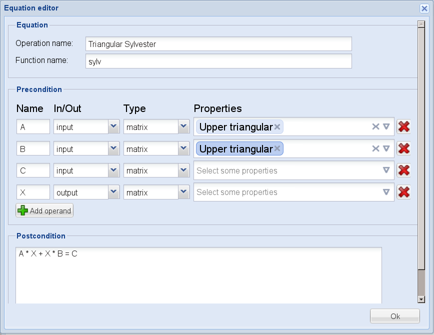
Figure 4.12: User-friendly web form to easily input the description of a target equation. In the example, we type the description of the Sylvester equation.

The second figure provides the output generated by the tool right after clicking the Ok button. It corresponds to the loop invariant number 7 from the third PME, i.e., the example used in Sections LABEL:subsec:pbef-paft and LABEL:subsec:updates. On the left-hand panel we find the PME and the loop invariant; on the right-hand panel we see the generated algorithm. We emphasize that, in contrast to the several days that it would take by hand, Cl1ck generated all 20 algorithms in only a few seconds.

Figure 4.13: Output from Cl1ck’s web interface for the input in Figure 4.12. On the left panel, the interface shows the equation itself, its PMEs, and its loop invariants; on the right panel, the interface displays the algorithms.

4.7 Scope and limitations

Given the mathematical definition of a target operation in terms of the predicates Precondition and Postcondition, Cl1ck produces a family of both algorithms and routines that compute it. Cl1ck has been applied to a broad set of linear algebra operations. We list a few examples:

• Vector-vector, matrix-vector, and matrix-matrix products (e.g., BLAS operations).

• Matrix factorizations, such as LU and Cholesky.

• Inversion of matrices.

• Operations arising in control theory, such as Lyapunov and Sylvester equations.

However, while it has been established that the information encoded in the PME suffices to generate algorithms [PaulDj:PhD], a precise characterization of the scope of the methodology, i.e., the class of operations that admit a PME, is still missing.

Beyond the scope of the methodology, Cl1ck presents a number of limitations similar to those discussed in Section LABEL:sec:clak-scope for Clak, i.e, the lack of: 1) a module to automatically select the best algorithms, 2) code generators for multiple programming languages and programming paradigms, and 3) a mechanism to analyze the stability of the produced algorithms. In this case, instead, promising work from Bientinesi et al. [Paolo-Stability] proposes an extension to the FLAME methodology for the systematic stability analysis of the generated algorithms. While still far fetched, this extension opens up the possibility for the future development of a module for the automatic stability analysis of Cl1ck-generated algorithms.

4.8 Summary

We presented Cl1ck, a prototype compiler for the automatic generation of loop-based linear algebra algorithms. From the sole mathematical description of a target equation, Cl1ck is capable of generating families of algorithms that solve it. To this end, Cl1ck adopts the FLAME methodology; the application of the methodology is divided in three stages: First, all PMEs for the target operation are generated; then, for each PME, multiple loop invariants are identified; finally, each loop invariant is used to build a provably correct algorithm. This chapter expands upon our work published in [CASC-2011-PME, ICCSA-2011-LINV].

The list of contributions made in this chapter follows.

• Minimum knowledge. For a given equation, we characterize the minimum knowledge required to automatically generate algorithms that solve it. This is the equation itself together with the properties of its operands.

• Full automation. We fully automate the generation of algorithms from the sole mathematical description of the operation. Previous work [PaulDj:PhD] required a PME and a loop invariant (both manually derived) as input, and the approach to automatically find the algorithm updates was limited.

• Feasibility. Several times this project has been deemed unfeasible. This chapter should serve as a precise reference on how to automate the process, and remove the skepticism.

For a wide class of linear algebra operations, the developers are now relieved from tedious, often unmanageable, symbolic manipulation, and only one Cl1ck separates them from the sought-after algorithms.

Chapter 5 Cl1ck: High-Performance Specialized Kernels

In the previous chapter, we demonstrated how Cl1ck automates the application of the FLAME methodology by means of multiple standard operations, such as the LU and Cholesky factorizations. While the application of Cl1ck to these operations shows the potential of the compiler, routines to compute them are already available from traditional libraries; in fact, most of the algorithms included in libFLAME [libflame] were derived using this methodology. In this chapter, instead, we concentrate on demonstrating the broad applicability of Cl1ck by generating customized kernels for building blocks not supported by standard numerical libraries.

When developing application libraries, it is not uncommon to require kernels for building blocks that are closely related but not supported by libraries like BLAS or LAPACK. The situation arises so often that extensions to traditional libraries are regularly proposed [2002:USB:567806.567807]; unfortunately, the inclusion of every possible kernel arising in applications is unfeasible. While it may be possible to emulate the required kernels via a mapping onto two or more available kernels, this approach typically affects both routine’s performance and developer’s productivity; alternatively, efficient customized kernels may be produced on demand. We illustrate this issue by means of two example kernels arising in the context of algorithmic differentiation.

Consider a program that solves a linear system of equations $AX=B$, with symmetric positive definite coefficient matrix $A$, and multiple right-hand sides $B$; pseudocode for such a program follows. First, $A$ is factored through a Cholesky factorization; then, two triangular linear systems are solved to compute the unknown $X$.

L LT= A (chol)L Y= B  (trsm)LTX= Y (trsm)

When interested in the derivative of this program, e.g., for a sensitivity analysis, one must compute the following sequence of derivative operations, dLdvLT+   L    dLTdv=   dAdv(gchol)dLdvY   +   L    dYdv=   dBdv(gtrsm)dLTdvX   +   LTdXdv=   dYdv, (gtrsm) none of which is supported by high-performance libraries. For both kernels, Cl1ck is capable of generating high-performance algorithms in a matter of seconds.

The aim of this chapter is two-fold: First, we use the operation gchol to provide a complete self-contained example of the application of Cl1ck, from the description of the operation to the final algorithms. Then, we present experimental results for both gchol and gtrsm; the corresponding routines attain high performance and scalability.

5.1 A complete example: The derivative of the Cholesky factorization

To initiate the derivation of algorithms for the derivative of the Cholesky factorization, Cl1ck requires the mathematical description of the operation. Given a symmetric positive definite matrix $A$, the Cholesky factorization calculates a lower triangular matrix $L$ such that

$$LL^{T}=A;$$ (5.1)

its derivative is dLdv    L^T   +    L    dLTdv    =    dAdv, where $L$ and $\frac{dA}{dv}$ are known, and $\frac{dL}{dv}$ is sought after. The quantities $L$ and $\frac{dL}{dv}$ are lower triangular matrices, and $\frac{dA}{dv}$ is a symmetric matrix. A formal description of the operation is given in Box 5.1; to simplify the notation and to avoid confusion, hereafter we replace $\frac{dA}{dv}$ and $\frac{dL}{dv}$ with $B$ and $G$, respectively.

G = gChol(L, B) ≡{ Ppre: {Output(G)   ∧  Input(L)   ∧Input(B)    ∧Matrix(G)   ∧  Matrix(L)   ∧Matrix(B)    ∧LowerTriangular(G)   ∧  LowerTriangular(L)    ∧Symmetric(B) } Ppost: {G LT+ L GT= B }

Box 5.1 Formal description for the derivative of the Cholesky factorization.

We recall that this description is the sole input required by Cl1ck to generate algorithms; all the actions leading to the algorithms in Figure LABEL:fig:gchol-algs are carried out automatically.

Pattern Learning

Given the description of gchol in Box 5.1, Cl1ck creates the pattern corresponding to gchol (Box 5.2), and incorporates it to its knowledge-base. The system is now capable of identifying gchol in the subsequent steps of the process.

        equal[
          plus[
            times[ G_, trans[L_] ],
            times[ L_, trans[G_] ]
          ],
          B_
        ] /;  isInputQ[L] && isInputQ[B] && isOutputQ[G] &&
              isMatrixQ[L] && isMatrixQ[B] && isMatrixQ[G] &&
              isLowerTriangularQ[L] && isSymmetricQ[B] &&
              isLowerTriangularQ[G]

Box 5.2 Mathematica pattern representing gchol.

5.1.1 Generation of the PME

In this initial stage, Cl1ck first identifies the feasible sets of partitionings for the operands; then, for each of these sets of partitionings, the system produces the corresponding partitioned postcondition, which gives raise to a number of equations; finally, these equations are matched against known patterns, yielding the PME(s).

Feasible Partitionings

To find the sets of valid partitionings for the operands, Cl1ck applies the algorithm described in Section LABEL:subsec:automation to the tree representation of gchol (Figure 5.1).

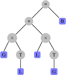
Figure 5.1: Tree representation of gchol.

The algorithm starts by creating a list of disjoint sets, one per dimension of the operands: [ { L_r }, { L_c }, { B_r }, { B_c }, { G_r }, { G_c } ]. The tree is traversed in postorder. Since $G$ is triangular, $G_{c}$ and $G_{r}$ are bound together —the only admissible partitionings for $G$ are $1\times 1$ and $2\times 2$—; similarly, the triangularity of $L$ imposes a binding between $L_{r}$ and $L_{c}$. The corresponding sets of dimensions are merged, resulting in: [ { L_r, L_c }, { B_r }, { B_c }, { G_r, G_c } ].

Next, the node for the transpose of $L$ is analyzed, not causing any binding. Hence, Cl1ck continues by studying the left-most “$\times$” operator. Its children, $G$ and $L^{T}$, are, respectively, of size $G_{r}\times G_{c}$ and $L_{c}\times L_{r}$; a binding between $G_{c}$ and $L_{c}$ is thus imposed: [ { L_r, L_c, G_r, G_c }, { B_r }, { B_c } ]. A similar analysis of the subtree corresponding to $L\times G^{T}$, yields no new bindings. Then, the “+” node is visited. The node’s children expressions are of size $G_{r}\times L_{r}$ and $L_{r}\times G_{r}$; no new bindings occur. Cl1ck now proceeds with the analysis of the node corresponding to $B$; due to the symmetry of $B$, the sets containing $B_{r}$ and $B_{c}$ are merged: [ { L_r, L_c, G_r, G_c }, { B_r, B_c } ]. Finally, the “$=$” operator, with left-hand side of size $G_{r}\times L_{r}$ and right-hand side of size $B_{r}\times B_{c}$, imposes the union of the remaining two sets of dimensions. The final list of sets consists of a single group of dimensions: [ { L_r, L_c, G_r, G_c, B_r, B_c } ].

Since the application of the identity rule ($1\times 1$) to all operands does not lead to a valid partitioned postcondition, the only set of feasible partitionings is the application of the $2\times 2$ rule to every operand:

$$\begin{aligned} B_{m\times m}\rightarrow&\left(\begin{array}[]{c@{\;\;}|@{\;\;}c}B_{TL}&B_{BL}^{T}\\ \hline\cr B_{BL}&B_{BR}\end{array}\right),\\ \small\textnormal{where }&B_{TL}\textnormal{ is }k\times k\end{aligned}\begin{aligned} L_{m\times m}\rightarrow&\left(\begin{array}[]{c@{\;\;}|@{\;\;}c}L_{TL}&0\\ \hline\cr L_{BL}&L_{BR}\end{array}\right),\\ \small\textnormal{where }&L_{TL}\textnormal{ is }k\times k\end{aligned}\begin{aligned} G_{m\times m}\rightarrow&\left(\begin{array}[]{c@{\;\;}|@{\;\;}c}G_{TL}&0\\ \hline\cr G_{BL}&G_{BR}\end{array}\right).\\ \small\textnormal{where }&G_{TL}\textnormal{ is }k\times k\end{aligned}$$

The newly created submatrices inherit a number of properties: $B_{TL}$ and $B_{BR}$ are square and symmetric; $B_{BL}$ and $B_{TR}$ are the transpose of one another; $L_{TL}$, $L_{BR}$, $G_{TL}$, and $G_{BR}$ are lower triangular; $L_{TR}$, and $B_{TR}$ are the zero matrix; and $L_{BL}$, and $G_{BL}$ present no structure. Cl1ck sets these properties and keeps track of them for future use.

Matrix Algebra and Pattern Matching

Next, the system replaces the operands in the postcondition by their partitioned counterparts, producing the partitioned postcondition

$$\footnotesize\left(\begin{array}[]{c@{\;\;}|@{\;\;}c}G_{TL}&0\\ \hline\cr G_{BL}&G_{BR}\end{array}\right)\left(\begin{array}[]{c@{\;\;}|@{\;\;}c}L^{T}_{TL}&L^{T}_{BL}\\ \hline\cr 0&L^{T}_{BR}\end{array}\right)+\left(\begin{array}[]{c@{\;\;}|@{\;\;}c}L_{TL}&0\\ \hline\cr L_{BL}&L_{BR}\end{array}\right)\left(\begin{array}[]{c@{\;\;}|@{\;\;}c}G^{T}_{TL}&G^{T}_{BL}\\ \hline\cr 0&G^{T}_{BR}\end{array}\right)=\left(\begin{array}[]{c@{\;\;}|@{\;\;}c}B_{TL}&B_{BL}^{T}\\ \hline\cr B_{BL}&B_{BR}\end{array}\right).$$

The expression is multiplied out and the “=” operator distributed, yielding three equations:

$$\left(\begin{array}[]{c@{\;\;}|@{\;\;}c}G_{TL}L^{T}_{TL}+L_{TL}G^{T}_{TL}=B_{TL}&*\\ \hline\cr G_{BL}L^{T}_{TL}+L_{BL}G^{T}_{TL}=B_{BL}&G_{BL}L^{T}_{BL}+G_{BR}L^{T}_{BR}+L_{BL}G^{T}_{BL}+L_{BR}G^{T}_{BR}=B_{BR}\end{array}\right).$$ (5.2)

The iterative process towards the PME starts. We recall the use of coloring to help the reader following the description: green and red are used to highlight the known and unknown operands, respectively. The operands $L$ and $B$ are input to gchol, and so are all sub-matrices resulting from their partitioning. $G$ and its parts are output quantities. All three equations in (5.2) are in canonical form —on the left-hand side appear only output terms, and on the right-hand side appear only input terms—. Hence, no initial algebraic manipulation is required:

$$\left(\begin{array}[]{c@{\;\;}|@{\;\;}c}{\color[rgb]{1.0,0.0,0.0}G_{TL}}{\color[rgb]{0,0.390625,0}L^{T}_{TL}}+{\color[rgb]{0,0.390625,0}L_{TL}}{\color[rgb]{1.0,0.0,0.0}G^{T}_{TL}}={\color[rgb]{0,0.390625,0}B_{TL}}&*\\ \hline\cr{\color[rgb]{1.0,0.0,0.0}G_{BL}}{\color[rgb]{0,0.390625,0}L^{T}_{TL}}+{\color[rgb]{0,0.390625,0}L_{BL}}{\color[rgb]{1.0,0.0,0.0}G^{T}_{TL}}={\color[rgb]{0,0.390625,0}B_{BL}}&{\color[rgb]{1.0,0.0,0.0}G_{BL}}{\color[rgb]{0,0.390625,0}L^{T}_{BL}}+{\color[rgb]{1.0,0.0,0.0}G_{BR}}{\color[rgb]{0,0.390625,0}L^{T}_{BR}}+{\color[rgb]{0,0.390625,0}L_{BL}}{\color[rgb]{1.0,0.0,0.0}G^{T}_{BL}}+{\color[rgb]{0,0.390625,0}L_{BR}}{\color[rgb]{1.0,0.0,0.0}G^{T}_{BR}}={\color[rgb]{0,0.390625,0}B_{BR}}\end{array}\right).$$ (5.3)

Cl1ck inspects (5.3) for known patterns. A gchol operation is found in the top-left quadrant: The operation matches the pattern in Box 5.2, $L_{TL}$ and $B_{TL}$ are known matrices, $G_{TL}$ is unknown, $G_{TL}$ and $L_{TL}$ are lower triangular, and $B_{TL}$ is symmetric. The equation is rewritten as the assignment $G_{TL}:=gChol(L_{TL},B_{TL})$, and the unknown quantity, $G_{TL}$, is labeled as computable and becomes known; this information is propagated to every appearance of the operand:

$$\left(\begin{array}[]{c@{\;\;}|@{\;\;}c}{\color[rgb]{0,0.390625,0}G_{TL}}:=gChol({\color[rgb]{0,0.390625,0}L_{TL}},{\color[rgb]{0,0.390625,0}B_{TL}})&*\\ \hline\cr{\color[rgb]{1.0,0.0,0.0}G_{BL}}{\color[rgb]{0,0.390625,0}L^{T}_{TL}}+{\color[rgb]{0,0.390625,0}L_{BL}}{\color[rgb]{0,0.390625,0}G^{T}_{TL}}={\color[rgb]{0,0.390625,0}B_{BL}}&{\color[rgb]{1.0,0.0,0.0}G_{BL}}{\color[rgb]{0,0.390625,0}L^{T}_{BL}}+{\color[rgb]{1.0,0.0,0.0}G_{BR}}{\color[rgb]{0,0.390625,0}L^{T}_{BR}}+{\color[rgb]{0,0.390625,0}L_{BL}}{\color[rgb]{1.0,0.0,0.0}G^{T}_{BL}}+{\color[rgb]{0,0.390625,0}L_{BR}}{\color[rgb]{1.0,0.0,0.0}G^{T}_{BR}}={\color[rgb]{0,0.390625,0}B_{BR}}\end{array}\right).$$ (5.4)

The bottom-left equation in (5.4) is not in canonical form anymore; a simple step of algebraic manipulation brings the equation back to canonical form:

$$\left(\begin{array}[]{c@{\;\;}|@{\;\;}c}{\color[rgb]{0,0.390625,0}G_{TL}}:=gChol({\color[rgb]{0,0.390625,0}L_{TL}},{\color[rgb]{0,0.390625,0}B_{TL}})&*\\ \hline\cr{\color[rgb]{1.0,0.0,0.0}G_{BL}}{\color[rgb]{0,0.390625,0}L^{T}_{TL}}={\color[rgb]{0,0.390625,0}B_{BL}}-{\color[rgb]{0,0.390625,0}L_{BL}}{\color[rgb]{0,0.390625,0}G^{T}_{TL}}&{\color[rgb]{1.0,0.0,0.0}G_{BL}}{\color[rgb]{0,0.390625,0}L^{T}_{BL}}+{\color[rgb]{1.0,0.0,0.0}G_{BR}}{\color[rgb]{0,0.390625,0}L^{T}_{BR}}+{\color[rgb]{0,0.390625,0}L_{BL}}{\color[rgb]{1.0,0.0,0.0}G^{T}_{BL}}+{\color[rgb]{0,0.390625,0}L_{BR}}{\color[rgb]{1.0,0.0,0.0}G^{T}_{BR}}={\color[rgb]{0,0.390625,0}B_{BR}}\end{array}\right).$$ (5.5)

The bottom-left equation is identified as a triangular system (trsm). The output operand, $G_{BL}$, is computable, and turns green in the bottom-right quadrant:

$$\left(\begin{array}[]{c@{\;\;}|@{\;\;}c}{\color[rgb]{0,0.390625,0}G_{TL}}:=gChol({\color[rgb]{0,0.390625,0}L_{TL}},{\color[rgb]{0,0.390625,0}B_{TL}})&*\\ \hline\cr{\color[rgb]{0,0.390625,0}G_{BL}}:=({\color[rgb]{0,0.390625,0}B_{BL}}-{\color[rgb]{0,0.390625,0}L_{BL}}{\color[rgb]{0,0.390625,0}G^{T}_{TL}}){\color[rgb]{0,0.390625,0}L^{-T}_{TL}}&{\color[rgb]{0,0.390625,0}G_{BL}}{\color[rgb]{0,0.390625,0}L^{T}_{BL}}+{\color[rgb]{1.0,0.0,0.0}G_{BR}}{\color[rgb]{0,0.390625,0}L^{T}_{BR}}+{\color[rgb]{0,0.390625,0}L_{BL}}{\color[rgb]{0,0.390625,0}G^{T}_{BL}}+{\color[rgb]{0,0.390625,0}L_{BR}}{\color[rgb]{1.0,0.0,0.0}G^{T}_{BR}}={\color[rgb]{0,0.390625,0}B_{BR}}\end{array}\right).$$ (5.6)

A step of algebraic manipulation takes place to reestablish the canonical form in the bottom-right equation, resulting in

$$\left(\begin{array}[]{c@{\;\;}|@{\;\;}c}{\color[rgb]{0,0.390625,0}G_{TL}}:=gChol({\color[rgb]{0,0.390625,0}L_{TL}},{\color[rgb]{0,0.390625,0}B_{TL}})&*\\ \hline\cr{\color[rgb]{0,0.390625,0}G_{BL}}:=({\color[rgb]{0,0.390625,0}B_{BL}}-{\color[rgb]{0,0.390625,0}L_{BL}}{\color[rgb]{0,0.390625,0}G^{T}_{TL}}){\color[rgb]{0,0.390625,0}L^{-T}_{TL}}&{\color[rgb]{1.0,0.0,0.0}G_{BR}}{\color[rgb]{0,0.390625,0}L^{T}_{BR}}+{\color[rgb]{0,0.390625,0}L_{BR}}{\color[rgb]{1.0,0.0,0.0}G^{T}_{BR}}={\color[rgb]{0,0.390625,0}B_{BR}}-{\color[rgb]{0,0.390625,0}G_{BL}}{\color[rgb]{0,0.390625,0}L^{T}_{BL}}-{\color[rgb]{0,0.390625,0}L_{BL}}{\color[rgb]{0,0.390625,0}G^{T}_{BL}}\end{array}\right).$$ (5.7)

One last equation remains to be identified. Since $L_{BR}$ and $G_{BR}$ are lower triangular, and the system can establish the symmetry of the right-hand side expression, $B_{BR}-G_{BL}L^{T}_{BL}-L_{BL}G^{T}_{BL}$, the equation is matched as a gchol. The output quantity, $G_{BR}$, becomes input. No equation is left, the process completes, and the PME for gchol (Box 5.3) is returned.

( G_TL := gChol( L_TL, B_TL)*G_BL := (B_BL - L_BL G^T_TL) L^-T_TLG_BR := gChol(L_BR, B_BR - G_BL L^T_BL - L_BL G^T_BL) )

Box 5.3 PME for the derivative of the Cholesky factorization.

PME Learning

Once the PME is found, Cl1ck generates and stores in its knowledge-base the rewrite rule displayed in Box 5.4, which states how to decompose a gchol problem with partitioned operands into multiple subproblems. We recall that this rule is essential for the flattening of the $P_{\rm before}$ and $P_{\rm after}$ predicates in later steps of the methodology.

$\left(\begin{array}[]{c@{\;\;}|@{\;\;}c}G_{TL}&0\\ \hline\cr G_{BL}&G_{BR}\end{array}\right)$ := gChol $\left(\left(\begin{array}[]{c@{\;\;}|@{\;\;}c}L_{TL}&0\\ \hline\cr L_{BL}&L_{BR}\end{array}\right),\left(\begin{array}[]{c@{\;\;}|@{\;\;}c}B_{TL}&B^{T}_{BL}\\ \hline\cr B_{BL}&B_{BR}\end{array}\right)\right)\longrightarrow$ ( G_TL := gChol( L_TL, B_TL )*G_BL := (B_BL - L_BL G^T_TL) L^-T_TLG_BR := gChol(L_BR, B_BR - G_BL L^T_BL - L_BL G^T_BL) )

Box 5.4 Rewrite rule associated to gchol’s PME.

5.1.2 Loop invariant identification

From the PME, multiple loop invariants are identified in three successive steps: First, the PME is decomposed into a set of tasks; then, a graph of dependencies among tasks is built; and finally, the feasible subsets of the graph are returned as valid loop invariants.

Decomposition into tasks

Cl1ck analyzes the assignments in each quadrant of the PME, and decomposes them into a series of tasks. The analysis commences from the top-left quadrant: $G_{TL}:=gChol(L_{TL},B_{TL})$. Since the right-hand side consists of a function whose input arguments are simple operands, no decomposition is required and the assignment is returned as a single task.

The next inspected assignment is $G_{BL}:=(B_{BL}-L_{BL}G^{T}_{TL})L^{-T}_{TL}$. No single pattern matches the right-hand side, which therefore must be decomposed. Similarly to the decomposition undergone by Clak in Chapter LABEL:ch:compiler, Cl1ck first matches the expression $G_{BL}:=B_{BL}-L_{BL}G^{T}_{TL}$ as a matrix-matrix product, and then identifies the remaining operation $G_{BL}:=G_{BL}L^{-T}_{TL}$ as the solution of a triangular system. The two operations are yielded as tasks.

One last assignment remains to be studied: $G_{BR}:=gChol(L_{BR},B_{BR}-G_{BL}L^{T}_{BL}-L_{BL}G^{T}_{BL})$. As in the top-left quadrant, it represents a gchol function; in this case, however, one of the input arguments is an expression. The decomposition is carried out in two steps: First, Cl1ck matches the expression $G_{BR}:=B_{BR}-G_{BL}L^{T}_{BL}-L_{BL}G^{T}_{BL}$ with the pattern associated to the BLAS 3 operation syr2k and returns it; then, the function $G_{BR}:=gChol(L_{BR},G_{BR})$ is yielded. The complete list of generated tasks is

1. $G_{TL}:=gChol(L_{TL},B_{TL})$

2. $G_{BL}:=B_{BL}-L_{BL}G^{T}_{TL}$

3. $G_{BL}:=G_{BL}L^{-T}_{TL}$

4. $G_{BR}:=B_{BR}-G_{BL}L^{T}_{BL}-L_{BL}G^{T}_{BL}$

5. $G_{BR}:=gChol(L_{BR},G_{BR})$

Graph of dependencies

A graph of dependencies among tasks is built; the analysis proceeds as follows (we recall the use of boldface to highlight the dependencies). The study commences with Task 1. A true dependency is found between Tasks 1 and 2: The output operand of Task 1, $G_{TL}$, appears as an input quantity to Task 2.

• ${\bf G_{TL}}:=gChol(L_{TL},B_{TL})$

• $G_{BL}:=B_{BL}-L_{BL}{\bf G^{T}_{TL}}.$

Next, Task 2 is inspected. Its output operand, $G_{BL}$, is an input for Task 3:

• ${\bf G_{BL}}:=B_{BL}-L_{BL}G^{T}_{TL}$

• $G_{BL}:={\bf G_{BL}}L^{-T}_{TL},$

which imposes another dependency from Task 2 to 3. Since $G_{BL}$ is also the output of Task 3, an output dependency occurs; the direction of the dependency is imposed during the decomposition of the assignment ($G_{BL}:=(B_{BL}-L_{BL}G^{T}_{TL})L^{-T}_{TL}$) that originated these tasks: to ensure a correct result, first Task 2 is computed, and then Task 3.

Two more true dependencies are found from Task 3 to 4,

• ${\bf G_{BL}}:=B_{BL}L^{-T}_{TL}$

• $G_{BR}:=B_{BR}-{\bf G_{BL}}L^{T}_{BL}-L_{BL}{\bf G^{T}_{BL}},$

and from Task 4 to 5

• ${\bf G_{BR}}:=B_{BR}-G_{BL}L^{T}_{BL}-L_{BL}G^{T}_{BL}$

• $G_{BR}:=gChol(L_{BR},{\bf G_{BR}}).$

As for Tasks 2 and 3, an output dependency also exists between Tasks 4 and 5; the direction is imposed by the decomposition: First the argument to the function is computed (Task 4), and then the function itself (Task 5).

Finally, the output of Task 5, $G_{BR}$ does not appear as input to any other task, and the analysis completes. The resulting graph of dependencies is depicted in Figure 5.2.

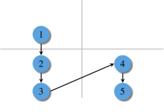
Figure 5.2: Task dependency graph obtained from the analysis of gchol’s PME.

Graph subsets selection

Predicates candidate to be loop invariants are selected as subsets of the graph that satisfy the dependencies. To obtain the subsets, Cl1ck utilizes Algorithm LABEL:alg:subDAG (Section LABEL:sec:depGraph). Since the application of the algorithm to gchol’s graph is rather straightforward, we skip the description and give the final list of subsets: [ {}, {1}, {1, 2}, {1, 2, 3}, {1, 2, 3, 4}, {1, 2, 3, 4, 5} ].

According to the rules stated in Chapter LABEL:ch:click, the predicates corresponding to the empty and full subgraphs are deemed not valid and discarded. The remaining four predicates lead to feasible loop invariants, which are collected in Table 5.1. In all four loop invariants, the three operands —$L$, $B$, and $G$— are traversed from the top-left to the bottom-right corner.

#	Subgraph	Loop-invariant
1		$\left(\begin{array}[]{@{\,}c@{\;\;}|@{\;\;}c@{\,}}G_{TL}:=gChol(L_{TL},B_{TL})&*\\ \hline\cr\hskip 42.9635pt\neq\hskip 42.9635pt\phantom{}&\qquad\,\neq\qquad\phantom{}\\ \end{array}\right)$
2		$\left(\begin{array}[]{c@{\;\;}|@{\;\;}c}G_{TL}:=gChol(L_{TL},B_{TL})&*\\ \hline\cr\hskip 9.95845ptG_{BL}:=B_{BL}-L_{BL}G^{T}_{TL}\hskip 9.95845pt\phantom{}&\qquad\,\neq\qquad\phantom{}\\ \end{array}\right)$
3		$\left(\begin{array}[]{c@{\;\;}|@{\;\;}c}G_{TL}:=gChol(L_{TL},B_{TL})&*\\ \hline\cr G_{BL}:=(B_{BL}-L_{BL}G^{T}_{TL})L^{-T}_{TL}&\qquad\,\neq\qquad\phantom{}\\ \end{array}\right)$
4		$\left(\begin{array}[]{c@{\;\;}|@{\;\;}c}G_{TL}:=gChol(L_{TL},B_{TL})&*\\ \hline\cr G_{BL}:=(B_{BL}-L_{BL}G^{T}_{TL})L^{-T}_{TL}&G_{BR}:=B_{BR}-G_{BL}L^{T}_{BL}-L_{BL}G^{T}_{BL}\end{array}\right)$

Table 5.1: Four loop invariants for the derivative of the Cholesky factorization.

5.1.3 Algorithm construction

The final stage in the generation of algorithms consists in constructing, for each loop invariant, the corresponding algorithm that computes gchol. The construction is carried out in three steps: 1) The repartitioning of the operands (Repartition and Continue with statements), 2) the rewrite of the loop invariant in terms of the repartitioned operands ($P_{\rm before}$ and $P_{\rm after}$ predicates), and 3) the comparison of these predicates to find the Algorithm Updates. We continue the example by means of gchol’s fourth loop invariant (Table 5.1).

Repartitioning of the operands

The loop invariant states that all three operands are traversed from top-left to bottom-right. This traversal must be captured by the Repartition and Continue with statements; Boxes 5.1.3 and 5.1.3, collect the corresponding Repartition and Continue with rules.

$\left(\begin{array}[]{c@{\;\;}I@{\;\;}c}L_{TL}\hfil\;\;\vrule width=&0\\ \cr\hline\cr\cr L_{BL}\hfil\;\;\vrule width=&L_{BR}\end{array}\right)\;\rightarrow\;\left(\begin{array}[]{c@{\;\;}I@{\;\;}c}(L_{00})\hfil\;\;\vrule width=&\left(\begin{array}[]{c@{\;\;}|@{\;\;}c}0&0\end{array}\right)\\ \cr\hline\cr\cr\left(\begin{array}[]{c}L_{10}\\ \hline\cr L_{20}\end{array}\right)\hfil\;\;\vrule width=&\left(\begin{array}[]{c@{\;\;}|@{\;\;}c}L_{11}&0\\ \hline\cr L_{21}&L_{22}\end{array}\right)\end{array}\right)$

(a)

$\left(\begin{array}[]{c@{\;\;}I@{\;\;}c}B_{TL}\hfil\;\;\vrule width=&B_{BL}^{T}\\ \cr\hline\cr\cr C_{BL}\hfil\;\;\vrule width=&B_{BR}\end{array}\right)\;\rightarrow\;\left(\begin{array}[]{c@{\;\;}I@{\;\;}c}(B_{00})\hfil\;\;\vrule width=&\left(\begin{array}[]{c@{\;\;}|@{\;\;}c}B_{10}^{T}&B_{20}^{T}\end{array}\right)\\ \cr\hline\cr\cr\left(\begin{array}[]{c}B_{10}\\ \hline\cr B_{20}\end{array}\right)\hfil\;\;\vrule width=&\left(\begin{array}[]{c@{\;\;}|@{\;\;}c}B_{11}&B_{21}^{T}\\ \hline\cr B_{21}&B_{22}\end{array}\right)\end{array}\right)$

(b)

$\left(\begin{array}[]{c@{\;\;}I@{\;\;}c}G_{TL}\hfil\;\;\vrule width=&0\\ \cr\hline\cr\cr G_{BL}\hfil\;\;\vrule width=&G_{BR}\end{array}\right)\;\rightarrow\;\left(\begin{array}[]{c@{\;\;}I@{\;\;}c}(G_{00})\hfil\;\;\vrule width=&\left(\begin{array}[]{c@{\;\;}|@{\;\;}c}0&0\end{array}\right)\\ \cr\hline\cr\cr\left(\begin{array}[]{c}G_{10}\\ \hline\cr G_{20}\end{array}\right)\hfil\;\;\vrule width=&\left(\begin{array}[]{c@{\;\;}|@{\;\;}c}G_{11}&0\\ \hline\cr G_{21}&G_{22}\end{array}\right)\end{array}\right)$

(c)

Box 5.5 Repartition rules for gchol’s fourth variant.

$\left(\begin{array}[]{c@{\;\;}I@{\;\;}c}L_{TL}\hfil\;\;\vrule width=&0\\ \cr\hline\cr\cr L_{BL}\hfil\;\;\vrule width=&L_{BR}\end{array}\right)\;\rightarrow\;\left(\begin{array}[]{c@{\;\;}I@{\;\;}c}\left(\begin{array}[]{c@{\;\;}|@{\;\;}c}L_{00}&0\\ \hline\cr L_{10}&L_{11}\end{array}\right)\hfil\;\;\vrule width=&\left(\begin{array}[]{c}0\\ \hline\cr 0\end{array}\right)\\ \cr\hline\cr\cr\left(\begin{array}[]{c@{\;\;}|@{\;\;}c}L_{20}&L_{21}\end{array}\right)\hfil\;\;\vrule width=&(L_{22})\end{array}\right)$

(a)

$\left(\begin{array}[]{c@{\;\;}I@{\;\;}c}B_{TL}\hfil\;\;\vrule width=&B_{BL}^{T}\\ \cr\hline\cr\cr B_{BL}\hfil\;\;\vrule width=&B_{BR}\end{array}\right)\;\rightarrow\;\left(\begin{array}[]{c@{\;\;}I@{\;\;}c}\left(\begin{array}[]{c@{\;\;}|@{\;\;}c}B_{00}&B_{10}^{T}\\ \hline\cr B_{10}&B_{11}\end{array}\right)\hfil\;\;\vrule width=&\left(\begin{array}[]{c}B_{20}^{T}\\ \hline\cr B_{21}^{T}\end{array}\right)\\ \cr\hline\cr\cr\left(\begin{array}[]{c@{\;\;}|@{\;\;}c}B_{20}&B_{21}\end{array}\right)\hfil\;\;\vrule width=&(B_{22})\end{array}\right)$

(b)

$\left(\begin{array}[]{c@{\;\;}I@{\;\;}c}G_{TL}\hfil\;\;\vrule width=&0\\ \cr\hline\cr\cr G_{BL}\hfil\;\;\vrule width=&G_{BR}\end{array}\right)\;\rightarrow\;\left(\begin{array}[]{c@{\;\;}I@{\;\;}c}\left(\begin{array}[]{c@{\;\;}|@{\;\;}c}G_{00}&0\\ \hline\cr G_{10}&G_{11}\end{array}\right)\hfil\;\;\vrule width=&\left(\begin{array}[]{c}0\\ \hline\cr 0\end{array}\right)\\ \cr\hline\cr\cr\left(\begin{array}[]{c@{\;\;}|@{\;\;}c}G_{20}&G_{21}\end{array}\right)\hfil\;\;\vrule width=&(G_{22})\end{array}\right)$

(c)

Box 5.6 Continue with rules for gchol’s fourth variant.

Predicates $P_{\rm before}$ and $P_{\rm after}$

To construct the $P_{\rm before}$ and $P_{\rm after}$ predicates, Cl1ck first rewrites the loop invariant in terms of the repartitioned operands. To this end, Cl1ck applies the Repartition and Continue with rules, producing, respectively, the top and bottom expressions in Figure 5.3. Then, these expressions are flattened out using both basic matrix algebra and the PME rewrite rule in Box 5.4. The final $P_{\rm before}$ and $P_{\rm after}$ predicates are also given in Figure 5.3.

$P_{\rm before}:$	$\left(\begin{array}[]{c@{\;\;}|@{\;\;}c}(G_{00}):=gChol((L_{00}),(B_{00}))&*\\ \hline\cr\left(\begin{array}[]{c}G_{10}\\ \hline\cr G_{20}\end{array}\right):=\left(\left(\begin{array}[]{c}B_{10}\\ \hline\cr B_{20}\end{array}\right)-\left(\begin{array}[]{c}L_{10}\\ \hline\cr L_{20}\end{array}\right)(G_{00})^{T}\right)(L_{00})^{-T}&\left(\begin{array}[]{c@{\;\;}|@{\;\;}c}G_{11}&0\\ \hline\cr G_{21}&G_{22}\end{array}\right):=\left(\begin{array}[]{c@{\;\;}|@{\;\;}c}B_{11}&B_{21}^{T}\\ \hline\cr B_{21}&B_{22}\end{array}\right)-\left(\begin{array}[]{c}G_{10}\\ \hline\cr G_{20}\end{array}\right)\left(\begin{array}[]{c}L_{10}\\ \hline\cr L_{20}\end{array}\right)^{T}-\left(\begin{array}[]{c}L_{10}\\ \hline\cr L_{20}\end{array}\right)\left(\begin{array}[]{c}G_{10}\\ \hline\cr G_{20}\end{array}\right)^{T}\end{array}\right)$
	$\Downarrow$ Flattening
	$\left(\begin{array}[]{c@{\;\;}|@{\;\;}c@{\;\;}|@{\;\;}c}G_{00}:=gChol(L_{00},B_{00})&0&0\\ \hline\cr G_{10}:=(B_{10}-L_{10}G^{T}_{00})L^{-T}_{00}&G_{11}:=B_{11}-G_{10}L^{T}_{10}-L_{10}G^{T}_{10}&0\\ \hline\cr G_{20}:=(B_{20}-L_{20}G^{T}_{00})L^{-T}_{00}&G_{21}:=B_{21}-G_{20}L^{T}_{10}-L_{20}G^{T}_{10}&G_{22}:=B_{22}-G_{20}L^{T}_{20}-L_{20}G^{T}_{20}\end{array}\right)$
	Algorithm Updates
$P_{\rm after}:$	$\left(\begin{array}[]{c@{\;\;}|@{\;\;}c@{\;\;}|@{\;\;}c}G_{00}:=gChol(L_{00},B_{00})&0&0\\ \hline\cr G_{10}:=(B_{10}-L_{10}G^{T}_{00})L^{-T}_{00}&G_{11}:=gChol(L_{11},B_{11}-G_{10}L^{T}_{10}-L_{10}G^{T}_{10})&0\\ \hline\cr G_{20}:=(B_{20}-L_{20}G^{T}_{00})L^{-T}_{00}&\begin{aligned} G_{21}:=(B_{21}&-B_{20}L^{-T}_{00}L^{T}_{10}+L_{20}G^{T}_{00}L^{-T}_{00}L^{T}_{10}\\ &-L_{20}G^{T}_{10}-L_{21}G^{T}_{11})L^{-T}_{11}\end{aligned}&\begin{aligned} G_{22}:=B_{22}&-G_{20}L^{T}_{20}-L_{20}G^{T}_{20}\\ &-G_{21}L^{T}_{21}-L_{21}G^{T}_{21}\end{aligned}\end{array}\right)$
	$\Uparrow$ Flattening
	$\left(\begin{array}[]{c@{\;\;}|@{\;\;}c}\left(\begin{array}[]{c@{\;\;}|@{\;\;}c}G_{00}&0\\ \hline\cr G_{10}&G_{11}\end{array}\right):=gChol\left(\left(\begin{array}[]{c@{\;\;}|@{\;\;}c}L_{00}&0\\ \hline\cr L_{10}&L_{11}\end{array}\right),\left(\begin{array}[]{c@{\;\;}|@{\;\;}c}B_{00}&B_{10}^{T}\\ \hline\cr B_{10}&B_{11}\end{array}\right)\right)&*\\ \hline\cr\left(\begin{array}[]{c@{\;\;}|@{\;\;}c}G_{20}&G_{21}\end{array}\right):=\left(\left(\begin{array}[]{c@{\;\;}|@{\;\;}c}B_{20}&B_{21}\end{array}\right)-\left(\begin{array}[]{c@{\;\;}|@{\;\;}c}L_{20}&L_{21}\end{array}\right)\left(\begin{array}[]{c@{\;\;}|@{\;\;}c}G_{00}&0\\ \hline\cr G_{10}&G_{11}\end{array}\right)^{T}\right)\left(\begin{array}[]{c@{\;\;}|@{\;\;}c}L_{00}&0\\ \hline\cr L_{10}&L_{11}\end{array}\right)^{-T}&\begin{aligned} (G_{22}):=(B_{22})&-\left(\begin{array}[]{c@{\;\;}|@{\;\;}c}G_{20}&G_{21}\end{array}\right)\left(\begin{array}[]{c@{\;\;}|@{\;\;}c}L_{20}&L_{21}\end{array}\right)^{T}\\ &-\left(\begin{array}[]{c@{\;\;}|@{\;\;}c}L_{20}&L_{21}\end{array}\right)\left(\begin{array}[]{c@{\;\;}|@{\;\;}c}G_{20}&G_{21}\end{array}\right)^{T}\end{aligned}\end{array}\right)$

Figure 5.3: $P_{\rm before}$ and $P_{\rm after}$ predicates for gchol’s fourth loop invariant.

Finding the updates

The final step undergone by Cl1ck consists in determining the updates that take the computation from the state in $P_{\rm before}$ to the state in $P_{\rm after}$.

The contents of both predicates only differ in quadrants $G_{11}$, $G_{21}$, and $G_{22}$. In the case of $G_{11}$ and $G_{22}$, the right-hand side of the expressions in $P_{\rm before}$ appear explicitly in the corresponding quadrants of $P_{\rm after}$. Hence, for those quadrants, a direct replacement suffices to obtain the required updates: G11:= gChol( L11, G11) G22:= G22- G21LT21- L21GT21.

The before state for $G_{21}$, instead, is not explicitly found in the after state; thus, both must be rewritten so that no redundant subexpressions appear. To avoid clutter, we anticipate that only the after state is rewritten; Cl1ck uses the rule from quadrant $G_{20}$: (B_20 - L_20 G^T_00) L^-T_00 →G_20, to rewrite the expression G_21 := (B_21 - B_20 L^-T_00 L^T_10 + L_20 G^T_00 L^-T_00 L^T_10 - L_20 G^T_10 - L_21 G^T_11) L^-T