Relativistic heavy-ion collisions

Abstract

The field of relativistic heavy-ion collisions is introduced to the high-energy physics students with no prior knowledge in this area. The emphasis is on the two most important observables, namely the azimuthal collective flow and jet quenching, and on the role fluid dynamics plays in the interpretation of the data. Other important observables described briefly are constituent quark number scaling, ratios of particle abundances, strangeness enhancement, and sequential melting of heavy quarkonia. Comparison is made of some of the basic heavy-ion results obtained at LHC with those obtained at RHIC. Initial findings at LHC which seem to be in apparent conflict with the accumulated RHIC data are highlighted.

1 Introduction

These are exciting times if one is working in the area of relativistic heavy-ion collisions, with two heavy-ion colliders namely the Relativistic Heavy-Ion Collider (RHIC) at the Brookhaven National Laboratory and the Large Hadron Collider (LHC) at CERN in operation in tandem. Quark-gluon plasma has been discovered at RHIC, but its precise properties are yet to be established. With the phase diagram of strongly interacting matter (QCD phase diagram) also being largely unknown, these are also great times for fresh graduate students to get into this area of research, which is going to remain very active for the next decade at least. The field is maturing as evidenced by the increasing number of text books that are now available [1, 2, 3, 4, 5, 6, 7, 8, 9]. Also available are collected review articles; see [10, 11, 12].

This is a fascinating inter-disciplinary area of research at the interface of particle physics and high-energy nuclear physics. It draws heavily from QCD — perturbative, non-perturbative, as well as semiclassical. It has overlaps with thermal field theory, relativistic fluid dynamics, kinetic or transport theory, quantum collision theory, apart from the standard statistical mechanics and thermodynamics. Quark-Gluon Plasma (QGP) at high temperature, $T$, and vanishing net baryon number density, $n_{B}$ (or equivalently the corresponding chemical potential, $\mu_{B}$), is of cosmological interest, while QGP at low $T$ and large $n_{B}$ is of astrophysical interest. String theorists too have developed interest in this area because of the black hole – fluid dynamics connection.

Students of high-energy physics would know that the science of the ‘small’ — the elementary particle physics — is deeply intertwined with the science of the ‘large’ — cosmology — the study of the origin and evolution of the universe. Figure 1 shows the temperature history of the universe starting shortly after the Big Bang. At times $\sim 10~{}\mu s$ after the Big Bang, with $T\mathrel{\hbox{\hbox to0.0pt{\lower 2.36806pt\hbox{$\sim$}\hss} \kern-3.00003pt\raise 1.72218pt\hbox{$>$}}}200$ MeV, the universe was in the state of QGP, and the present-day experiments which collide two relativistic heavy ions — the Little Bang — try to recreate that state of matter in the laboratory for a brief period of time.

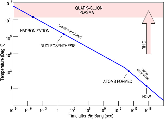
Figure 1: Temperature history of the universe. The Big Bang and the Little Bang.

Recall the phase diagram (pressure vs temperature) of water, Fig. 2(a). It shows three broad regions separated by phase transition lines, the triple point where all three phases coexist, and the critical point where the vapour pressure curve terminates and two distinct coexisting phases, namely liquid and gas, become identical. All these features are well-established experimentally to a great accuracy. In contrast the QCD phase diagram (Fig. 2(b)) is known only schematically, except for the lattice QCD predictions at vanishing or small $\mu_{B}$, in particular the prediction of a crossover transition around $T\sim 150$-170 MeV [14, 15] for vanishing $\mu_{B}$. As arguments based on a variety of models indicate a first-order phase transition as a function of temperature at finite $\mu_{B}$, one expects the phase transition line to end at a critical point. The existence of the critical point, however, is not established experimentally. Apart from the region of hadrons at the low enough $T$ and $\mu_{B}$, and the region of quarks and gluons at high $T$ and $\mu_{B}$, there is also a region characterized by colour superconductivity, at high $\mu_{B}$ and low $T$ [16, 17, 18]. However, precise boundaries separating these regions are not known experimentally. Actually the QCD phase diagram may be richer than what is shown in Fig. 2(b) [19]. Before we proceed further, a precise definition of QGP is in order. We follow the definition proposed by the STAR collaboration at RHIC: Quark-Gluon Plasma is defined as a (locally) thermally equilibrated state of matter in which quarks and gluons are deconfined from hadrons, so that they propagate over nuclear, rather than merely nucleonic, volumes [20]. Note the two essential ingredients of this definition, (a) the constituents of the matter should be quarks and gluons, and (b) the matter should have attained (local) thermal equilibrium. Any claim of discovery of QGP can follow only after these two requirements are shown to be fulfilled unambiguously.

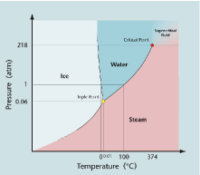
Figure 2: (a) Phase diagram of water [13] and (b) QCD phase diagram

The big idea thus is to map out (quantitatively) the QCD phase diagram [21]. The main theoretical tool at our disposal is, of course, the lattice QCD. Although it allows first-principle calculations, it has technical difficulties for non-vanishing $\mu_{B}$ or $n_{B}$. We also have various effective theories and phenomenological models which indeed are the basis of the schematic phase diagram of QCD shown in Fig. 2(b). Experimental tools available to us are the relativistic heavy-ion colliders such as those at BNL and CERN, and the upcoming lower-energy facilities namely Facility for Antiproton and Ion Research (FAIR) at GSI and Nuclotron-based Ion Collider fAcility (NICA) at JINR. Apart from these terrestrial facilities, astronomy of neutron stars can also throw light on the low $T$ and high $n_{B}$ region of the QCD phase diagram.

Figure 3 shows the lattice results for the QCD equation of state (EoS) at vanishing chemical potential in the temperature range $100~{}{\textmd{M}eV}\mathrel{\hbox{\hbox to0.0pt{\lower 2.36806pt\hbox{$\sim$}\hss} \kern-3.00003pt\raise 1.72218pt\hbox{$<$}}}T\mathrel{\hbox{\hbox to0.0pt{\lower 2.36806pt\hbox{$\sim$}\hss} \kern-3.00003pt\raise 1.72218pt\hbox{$<$}}}1000$ MeV for physical light and strange quark masses $m_{u,d,s}$. Note that both energy density ($\epsilon$) and pressure ($P$) rise rapidly around $T=160$ MeV, indicating an increase in entropy or the number of degrees of freedom. This is consistent with the deconfinement transition with a concomitant release of the partonic degrees of freedom. The rise of $P$ is less rapid than that of $\epsilon$ as expected: the square of the speed of sound $c_{s}^{2}=\partial P/\partial\epsilon$ cannot exceed unity. Note also that in the limit of high $T$, the EoS approaches the form $\epsilon=3P$ expected of massless particles. However, $\epsilon$ is significantly less than $\epsilon_{SB}$ showing that the system is far from being in an ideal gaseous state. Lattice results indicate that the transition at vanishing $\mu_{B}$ is merely an analytic crossover. Although there is no strict phase transition, it is common to use the words confined and deconfined phases to describe the low- and high-temperature regimes. For a recent review of the lattice QCD at non-zero temperature, see [22].

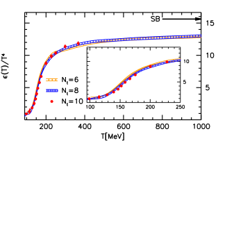
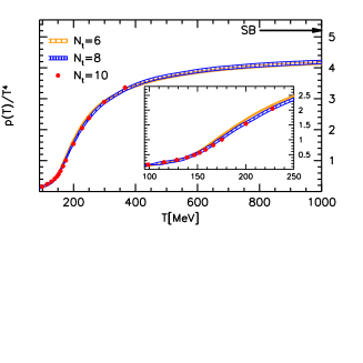
Figure 3: Energy density and pressure normalized by $T^{4}$ as a function of temperature ($T$) on $N_{t}$ = 6, 8 and 10 lattices. $N_{t}$ is the number of lattice points in the temporal direction. The Stefan-Boltzmann (SB) limits are indicated by arrows. Figure from [14]; see also [15].

An ultrarelativistic heavy-ion collision (URHIC) of two (identical) Lorentz-contracted nuclei is thought to proceed as follows. Each incoming nucleus can be looked upon as a coherent [5] cloud of partons (more precisely, a colour-glass-condensate (CGC) plate [24]). The collision results in shattering of the two CGC plates. A significant fraction of the incoming kinetic energy is deposited in the central region leading to a high-energy-density fireball (more precisely, a highly non-equilibrium state called glasma [24]). This is still a coherent state and liberation of partons from the glasma takes a finite amount of (proper) time (a fraction of a fm$/c$). Subsequently collisions among partons lead to a nearly thermalized (local thermalization!) state called QGP. This happens at a time of the order of 1 fm$/c$ — a less understood aspect of the entire process. Due to near thermalization, the subsequent evolution of the system proceeds as per relativistic imperfect fluid dynamics. This involves expansion, cooling, and dilution. Eventually the system hadronizes. Hadrons continue to collide among themselves elastically which changes their energy-momenta, as well as inelastically which alters abundances of individual species. Chemical freezeout occurs when inelastic processes stop. Kinetic freezeout occurs when elastic scatterings too stop. These late stages of evolution when the system is no longer in local equilibrium are simulated using the relativistic kinetic theory framework. Hadrons decouple from the system approximately 10-15 fm$/c$ after the collision and travel towards the surrounding detectors. From the volume of experimental data thus collected one has to establish whether QGP was formed and if so, extract its properties.

After years of work a Standard Model of URHICs has emerged: The initial state is constructed using either the Glauber model [25] or one of the models implementing ideas originating from CGC [26]; for a recent review see [27]. The intermediate evolution is considered using some version of the Müller-Israel-Stewart-like theory [28, 29] of causal relativistic imperfect fluid dynamics, together with a QCD equation of state spanning partonic and hadronic phases [30]. The end evolution of the hadron-rich medium leading to a freezeout uses the Boltzmann equation in the relativistic transport theory [31]. The final state consists of thousands of particles (mesons, baryons, leptons, photons, light nuclei). Detailed measurements (single-particle inclusive, two- and multi-particle correlations, etc.) are available, spanning the energy range from SPS to RHIC to LHC, for various colliding nuclei, centralities, (pseudo)rapidities, and transverse momenta. The aim is to achieve a quantitative understanding of the thermodynamic and transport properties of QGP, its EoS, its transport coefficients (shear and bulk viscosities, diffusivity, conductivity), etc. The major hurdles in this endeavour are an inadequate knowledge of the initial state and event-to-event fluctuations at nucleonic and sub-nucleonic levels in the initial state.

2 Two most important observables

Elliptic flow and jet quenching are arguably the two most important observables in this field. Observation of an elliptic flow almost as large as that predicted by ideal (equilibrium) hydrodynamics led to the claim of formation of an almost perfect fluid at RHIC [32]. A natural explanation of the observed jet quenching is in terms of a dense and coloured (hence partonic, not hadronic) medium that is rather opaque to high-momentum hadrons. Recall the definition of QGP given in section 1. The two essential requirements mentioned there seem to be fulfilled considering these two observations together.

Before I discuss these two observations in detail, let me explain what is meant by an almost perfect fluid. Air and water are the two most common fluids we encounter. Which of them is more viscous? Water has a higher coefficient of shear viscosity ($\eta$) than air, and appears more viscous. But that is misleading. To compare different fluids, one should consider their kinematic viscosities defined as $\eta/\rho$ where $\rho$ is the density. Air has a higher kinematic viscosity and hence is actually more viscous than water! Relativistic analogue of $\eta/\rho$ is the dimensionless ratio $\eta/s$ where $s$ is the entropy density. Scaling by $s$ is appropriate because number density is ill-defined in the relativistic case. Figure 4 shows constant-pressure ($P_{critical}$) curves for $\eta/s$ as a function of temperature for various fluids, namely water, nitrogen, helium, and the fluid formed at RHIC. All fluids show a minimum at the critical temperature, and among them the RHIC fluid has the lowest $\eta/s$, even lower than that of helium. Hence it is the most perfect fluid observed so far. For water, nitrogen, and helium, points to the left (right) of the minimum refer to the liquid (gaseous) phase. As $T$ rises, $\eta/s$ for these liquids drops, attains a minimum at the critical temperature $T_{0}$, and then in the gaseous phase it rises. This is because liquids and gases transport momentum differently [35]. RHIC fluid is an example of a strongly coupled quantum fluid and has been called sQGP to distinguish it from weakly coupled QGP or wQGP expected at extremely high temperatures. Interestingly, the liquid formed at RHIC and LHC cools into a (hadron resonance) gas!

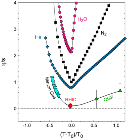
Figure 4: Constant pressure ($P_{critical}$) curves for (shear viscosity/entropy density) vs temperature. $T_{0}$ is the critical temperature of the liquid-gas phase transition. Points labelled Meson Gas are based on chiral perturbation theory and have $50\%$ errors (not shown). Points labelled QGP are based on lattice QCD simulations. Figure from [33].

2.1 Elliptic flow

Consider a non-central (non-zero impact parameter) collision of two identical spherical nuclei travelling in opposite directions; see Fig. 5(a). In an actual experiment the magnitude and orientation of the impact parameter vector fluctuate from event to event (Fig. 5(b)) and are unknown. This initial geometry can potentially affect the distribution of particles in the final state — in particular, in the transverse plane. In order to capture this physics in terms of a few parameters, the triple differential invariant distribution of particles emitted in the final state is Fourier-decomposed as follows [36]

$$E\frac{d^{3}N}{d^{3}p}=\frac{d^{3}N}{p_{T}dp_{T}dyd\phi}=\frac{d^{2}N}{p_{T}dp_{T}dy}\frac{1}{2\pi}\left[1+\sum_{n=1}^{\infty}2v_{n}\cos n(\phi-\Phi_{R})\right],$$ (1)

where $p_{T}$ is the transverse momentum, $y$ the rapidity, $\phi$ the azimuthal angle of the outgoing particle momentum, and $\Phi_{R}$ the reaction-plane angle. Sine terms, $\sin n(\phi-\Phi_{R})$, are not included in the Fourier expansion in Eq. (1) because they vanish due to the reflection symmetry with respect to the reaction plane; see Fig. 5. The reaction-plane angle $\Phi_{R}$ which characterizes the initial geometry (Fig. 5(b)) is not known, and is estimated using the transverse distribution of particles in the final state. The estimated reaction plane is called the event plane. The leading term in the square brackets in Eq. (1) represents the azimuthally symmetric radial flow. The first two harmonic coefficients $v_{1}$ and $v_{2}$ are called directed and elliptic flows, respectively. We have

$$v_{n}(p_{T},y)=\left\langle\cos[n(\phi-\Phi_{R})]\right\rangle=\frac{\int^{2\pi}_{0}d\phi\cos[n(\phi-\Phi_{R})]\frac{d^{3}N}{p_{T}dp_{T}dyd\phi}}{\int^{2\pi}_{0}d\phi\frac{d^{3}N}{p_{T}dp_{T}dyd\phi}}.$$ (2)

The average is taken in the $(p_{T},y)$ bin under consideration. After taking the average over all particles in an event, average is then taken over all events in a centrality class. For a central collision the azimuthal distribution is isotropic, and hence $v_{n}=0$, only the radial flow survives. For a review of the methods used for analyzing anisotropic flow in relativistic heavy-ion collisions, and interpretations and uncertainties in the measurements, see [37, 38].

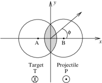
Figure 5: (a) Non-central collision of two nuclei. Collision or beam axis is perpendicular to the plane of the figure. Impact parameter $b$ = length AB. $z$ is the longitudinal direction, $xy$ is the transverse or azimuthal plane, $xz$ is the reaction plane, and $\phi$ is the azimuthal angle of one of the outgoing particles. The shaded area indicates the overlap zone. For a central or head-on collision ($b=0$) the reaction plane cannot be defined. (b) $XYZ$ are the lab-fixed axes. $\Phi_{R}$ is the reaction-plane angle.

In a non-central collision, the initial state is characterized by a spatial anisotropy in the azimuthal plane (Fig. 5). Consider particles in the almond-shaped overlap zone. Their initial momenta are predominantly longitudinal. Transverse momenta, if any, are distributed isotropically. If these particles do not interact with each other, the final (azimuthal) distribution too will be isotropic. On the other hand, if they do interact with each other frequently and with adequate strength (or cross section), then the (local) thermal equilibrium is likely to be reached. Once that happens, the system can be described in terms of thermodynamic quantities such as temperature, pressure, etc. The spatial anisotropy of the overlap zone ensures anisotropic pressure gradients in the transverse plane. This leads to a final state characterized by momentum anisotropy, an anisotropic azimuthal distribution of particles, and hence a nonvanishing $v_{n}$. Thus $v_{n}$ is a measure of the degree of thermalization of the quark-gluon matter produced in a noncentral heavy-ion collision — a central issue in this field.

The anisotropic flow $v_{n}$ is sensitive to the early ($\sim$ fm/$c$) history of the collision: Higher pressure gradients along the minor axis of the spatially anisotropic source (Fig. 5) imply that the expansion of the source would gradually diminish its anisotropy, making the flow self-quenching. Thus $v_{n}$ builds up early (when the anisotropy is significant) and tends to saturate as the anisotropy continues to decrease. (This is unlike the radial flow which continues to grow until freezeout and is sensitive to early- as well as late-time history of the collision). Thus $v_{n}$ is a signature of pressure at early times.

The flow $v_{n}$ depends on the initial conditions, the beam energy, the mass number of colliding nuclei, and the centrality of the collision. It also depends on the species of the particles under consideration apart from their transverse momentum $(p_{T})$ and rapidity $(y)$ or pseudorapidity $(\eta)$. Using the symmetry of the initial geometry, one can show that $v_{n}(y)$ is an even (odd) function of $y$ if $n$ is even (odd). Hence $v_{1}(y)$

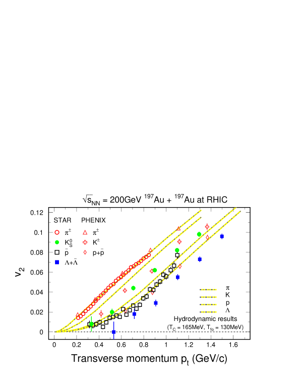
Figure 6: Success of ideal hydrodynamics: Minimum-bias elliptic flow data for different particle species in comparison with ideal hydrodynamics calculations. Figure from [39].

vanishes at mid-rapidity. At RHIC energies at mid-rapidity, it is the elliptic flow $v_{2}$ that plays an important role. Figure 6 shows the $v_{2}(p_{T})$ data at the highest RHIC energy for various particle species, in broad agreement with the ideal hydrodynamic calculations. As stated before, this success of the ideal hydrodynamics led to the claim of formation of an almost perfect fluid at RHIC.

Extraction of $\eta/s$: Introduction of shear viscosity tends to reduce the elliptic flow, $v_{2}$, with respect to that for an ideal fluid: a particle moving in the reaction plane (Fig. 5(a)) being faster experiences a greater frictional force compared with a particle moving out of the plane thereby reducing the azimuthal anisotropy and hence $v_{2}$. This fact has been used to place an upper limit on the value of $\eta/s$ of the RHIC fluid. A more precise determination is hindered by ambiguities in the knowledge of the initial state. Event-to-event fluctuations give rise to ‘new’ flows and observables which help constrain the $\eta/s$ further.

2.1.1 Event-to-event fluctuations

The discussion above was somewhat idealistic because we assumed smooth initial geometry: Energy (or entropy) density $\epsilon(x,y)$ $(\textrm{or}~{}s(x,y))$ in the shaded area in Fig. 5(a) was a smooth function of $x,y$ because it was assumed to result from the overlap of two smooth Woods-Saxon nuclear density distributions. However, the reality is not so simple, the initial geometry is not smooth.

In relativistic heavy-ion collisions, the collision time-scale is so short that each incoming nucleus sees nucleons in the other nucleus in a frozen configuration. Event-to-event fluctuations in nucleon ($N$) positions (and hence in $NN$ collision points) result in an overlap zone with inhomogeneous energy density and a shape that fluctuates from event to event, Fig. 7. This necessitates that the “sine terms” are also included in the Fourier expansion in Eq. (1). Equivalently, one writes

$$E\frac{d^{3}N}{d^{3}p}=\frac{d^{3}N}{p_{T}dp_{T}dyd\phi}=\frac{d^{2}N}{p_{T}dp_{T}dy}\frac{1}{2\pi}\left[1+\sum_{n=1}^{\infty}2v_{n}\cos n(\phi-\Psi_{n})\right].$$ (3)

Thus each harmonic $n$ may have its own reference angle $\Psi_{n}$ in the transverse plane. Traditional hydrodynamic

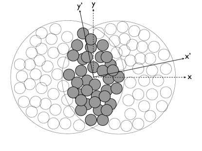
Figure 7: ‘Snapshot’ of nucleon positions at the instant of collision. Due to event-to-event fluctuations, the overlap zone could be shifted and tilted with respect to the $(x,y)$ frame. $x^{\prime}y^{\prime}$: principal axes of inertia. Figure from [40].

calculations do not take these event-to-event fluctuations into account. Instead of averaging over the fluctuating initial conditions and then evolving the resultant smooth distribution, one needs to perform event-to-event hydrodynamics calculations first and then average over all outputs. This is done in some of the recent hydrodynamic calculations. They also incorporate event-to-event fluctuations at the sub-nucleonic level. Fluctuating initial geometry results in ‘new’ (rapidity-even) flows (Fig. 8). The rapidity-even dipolar flow shown in Fig. 8(a) is not to be confused with the rapidity-odd directed flow $v_{1}(p_{T},y)$ resulting from the smooth initial geometry in Fig. 5.

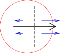
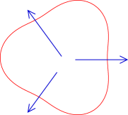
Figure 8: (a) Dipole asymmetry giving rise to a dipolar flow $v_{1}(p_{T},y)$. The cross indicates the centre of entropy (analogous to the centre of mass) and the large arrow indicates the orientation of the dipole. (b)Triangularity giving rise to a triangular flow $v_{3}(p_{T},y)$. Figure from [41].

For recent reviews of the collective flow, its anisotropies, its event-to-event fluctuations, and the extraction of the specific shear viscosity $\eta/s$ of QGP, see [42, 43, 44].

2.2 Jet quenching

Recall the role played by successively higher-energy electron beams, over many decades in the last century, to unravel the structure of atoms, nuclei, and protons. Studying the properties of QGP by means of an external probe is obviously ruled out because of its short ($\sim 10^{-23}$ s) life-time. Instead one uses a hard parton produced internally during the nucleus-nucleus collision to probe the medium in which it is produced. Consider, $g+g\rightarrow g+g$ where two longitudinally moving energetic gluons from the colliding nuclei interact and produce two gluons at large transverse momenta, which fragment and emerge as jets of particles. Hard partons are produced early in the collision: $t\sim 1/Q\sim 1/p_{T}$, where $Q$ is the parton virtuality scale, and hence they probe the early stages of the collision. Moreover, their production rate is calculable in perturbative QCD. Parton/jet interacts with the medium and loses energy or gets quenched as it traverses the medium (Fig. 9(a)). The amount of energy loss depends among other things on the path length ($L$) the jet has to travel inside the medium. Figure 9(b) shows the data on the nuclear modification factor, $R_{AA}$, defined schematically as

$$R_{AA}(p_{T})=\textrm{Yield ~{}in~{}}AA/\left\langle N_{coll}\right\rangle\textrm{Yield~{} in~{}}pp,$$ (4)

where $\left\langle N_{coll}\right\rangle$ is the mean number of nucleon-nucleon collisions occurring in a single nucleus-nucleus ($AA$) collision, obtained within the Glauber model [25]. If the nucleus-nucleus collision were a simple superposition of nucleon-nucleon collisions, the ratio $R_{AA}$ would be unity. Direct-photon production rate is consistent with the next-to-leading-order (NLO) perturbative QCD (pQCD) calculation and there is no suppression of the photon yield. However, the yields of high-$p_{T}$ pions and etas are suppressed by a factor of $\sim 5$. No such suppression was seen in $d$Au and $p$Pb collisions [49] (where QGP is not expected to be formed) thereby ruling out suppression by cold nuclear matter as the cause. These observations indicate that the hard-scattered partons lose energy as they traverse the hot medium and the suppression is thus a final-state effect.

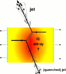
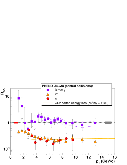
Figure 9: (a) Back-to-back jets, one produced near the surface of the hot and dense medium and the other deep inside. These are called the near-side and away-side jets. The latter gets quenched. The medium is characterized by its temperature ($T$), gluon number density in the rapidity space ($dN^{g}/dy$), and the transport coefficient or jet-quenching parameter ($\hat{q}$). Figure from [45]. (b) AuAu central collision data on nuclear modification factor $R_{AA}$ as a function of $p_{T}$, at the centre-of-mass energy $\sqrt{s_{NN}}=200$ GeV. Dash-dotted lines: theoretical uncertainties in the direct photon $R_{AA}$. Solid yellow line: jet-quenching calculation of [46, 47] for leading pions in a medium with initial effective gluon density $dN^{g}/dy=1100$. Error bands at $R_{AA}=1$ indicate the absolute normalization errors. Figure from [48].

Figure 9(b) illustrated jet quenching in a single-particle inclusive yield. Jet quenching is also seen in dihadron angular correlations shown in Fig. 10 as a function of the opening angle between the trigger and associated particles. The only difference between the left and the right panels is the definition of the associated particles. The left panel shows the suppression of the away-side jet in AuAu central, but not in $pp$ and $d$Au central collisions. This is expected because unlike AuAu collisions, no hot and dense medium is likely to be formed in $pp$ and $d$Au collisions, and so there is no quenching of the away-side jet. Energy of the away-side parton in a AuAu collision is dissipated in the medium thereby producing low-$p_{T}$ or soft particles. When even the soft particles are included, the away-side jet reappears in the AuAu data as shown in the right panel. Its shape is broadened due to interactions with the medium.

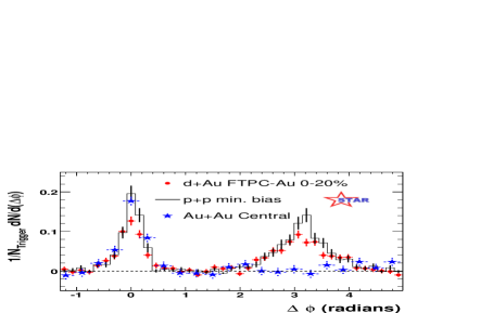
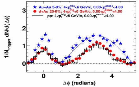
Figure 10: (a) STAR data on dihadron angular correlations. $\Delta\phi$ is the opening angle between the trigger ($4<p_{T}^{trig}<6$ GeV$/c$) and associated particles ($2<p_{T}^{assoc}<p_{T}^{trig}$ GeV$/c$). Figure from [50]. (b) Similar to the left panel, except that $0<p_{T}^{assoc}<4$ GeV$/c$. Figure from [51].

Figure 11 shows two main mechanisms by which a parton moving in the medium loses energy. Collisional energy loss via elastic scatterings dominates at low momenta whereas the radiative energy loss via inelastic scatterings dominates at high momenta. Energy loss per unit path length depends on the properties of the parton (parton species, energy $E$), as well as the properties of the medium ($T,~{}dN^{g}/dy,~{}\hat{q}$). The jet quenching parameter, $\hat{q}$, is defined as the average $p_{T}^{2}$ transferred to the outgoing parton per unit path length. The value of $\hat{q}$ estimated in leading-order QCD is $\simeq 2.2$ GeV²/fm, while the value extracted from phenomenological fits to the RHIC experimental data on parton energy loss is $\mathcal{O}(10)$ GeV²/fm.

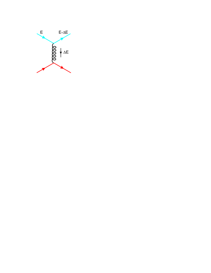
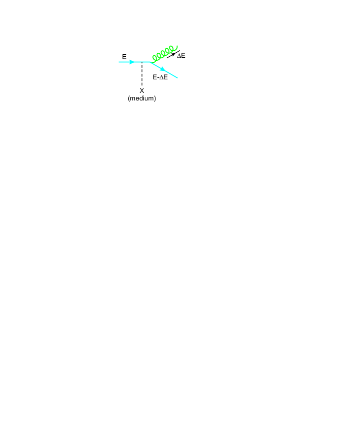
Figure 11: Collisional (left) and medium-induced radiative (right) energy loss mechanisms. Their predictions for the energy loss per unit length differ from each other: $\Delta E\propto L$ and $\Delta E\propto L^{2}$, respectively. Figure from [45].

Jets are more abundant and easier to reconstruct at LHC than at RHIC. Figure 12 shows an example of an unbalanced dijet in a PbPb collision event at CMS (LHC). By studying the evolution of the dijet imbalance as a function of collision centrality and energy of the leading jet, one hopes to get an insight into the dynamics of the jet quenching.

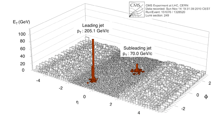
Figure 12: Jet quenching in PbPb collision at the centre-of-mass energy $\sqrt{s_{NN}}=2.76$ TeV at CMS. $E_{T}$ is the summed transverse energy in the electromagnetic and hadron calorimeters. $\eta$ and $\phi$ are the pseudorapidity and azimuthal angle, respectively. Figure from [52].

For recent reviews of jet quenching, see [53, 45, 54, 55].

3 Some other important observables

Elliptic flow, or more generally anisotropic collective flow, and jet quenching, which we discussed above are examples of soft and hard probes, respectively. Here ‘soft’ refers to the low-$p_{T}$ regime: $0\mathrel{\hbox{\hbox to0.0pt{\lower 2.36806pt\hbox{$\sim$}\hss} \kern-3.00003pt\raise 1.72218pt\hbox{$<$}}}p_{T}\mathrel{\hbox{\hbox to0.0pt{\lower 2.36806pt\hbox{$\sim$}\hss} \kern-3.00003pt\raise 1.72218pt\hbox{$<$}}}1.5$ GeV$/c$, and hard refers to high-$p_{T}$ regime: $p_{T}\gg 5$ GeV$/c$. (At RHIC, such high-$p_{T}$ jets are rare, which explains the relatively low $p_{T}$ cuts used in Fig. 10.) The medium-$p_{T}$ regime ($1.5\mathrel{\hbox{\hbox to0.0pt{\lower 2.36806pt\hbox{$\sim$}\hss} \kern-3.00003pt\raise 1.72218pt\hbox{$<$}}}p_{T}\mathrel{\hbox{\hbox to0.0pt{\lower 2.36806pt\hbox{$\sim$}\hss} \kern-3.00003pt\raise 1.72218pt\hbox{$<$}}}5$ GeV$/c$) is also interesting, for the phenomenon of constituent quark number scaling or quark coalescence. In this section we discuss briefly this and other important observables. We shall, however, not discuss a few other important topics such as femtoscopy with two-particle correlation measurements [56, 57, 58] and electromagnetic probes of QGP [59, 60].

3.1 Constituent quark number scaling

In the high-$p_{T}$ regime, hadronization occurs by fragmentation, whereas in the medium-$p_{T}$ regime, it is modelled by quark recombination or coalescence. The phenomenon of constituent quark number scaling provides experimental support to this model. Figure 13 explains the meaning of constituent quark number ($n_{q}$) scaling. In the left panel one sees two distinct branches, one for baryons ($n_{q}=3$) and the other for mesons ($n_{q}=2$). When scaled by $n_{q}$ (right panel), the two curves merge into one universal curve, suggesting that the flow is developed at the quark level, and hadrons form by the merging of constituent quarks. This observation provides the most direct evidence for deconfinement so far. ALICE (LHC) has also reported results for the elliptic flow $v_{2}(p_{T})$ of identified particles produced in PbPb collisions at 2.76 TeV. The constituent quark number scaling was found to be not as good as at RHIC [62].

For a recent review see [63].

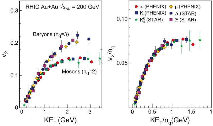
Figure 13: (Left) Elliptic flow $v_{2}$ vs transverse kinetic energy $KE_{T}$ for various baryons and mesons. (Right) Both $v_{2}$ and $KE_{T}$ are scaled by the number of constituent quarks $n_{q}$. Figure from [61].

3.2 Ratios of particle abundances

Ratios of particle abundances such as $K/\pi,~{}p/\pi$, etc. constrain models of particle production. In the thermal or statistical hadronization model [64, 65], particles in the final state are assumed to be emitted by a source in a thermodynamic equilibrium characterized by only a few parameters such as the (chemical freezeout) temperature and the baryo-chemical potential. These parameters are determined by fitting the experimental data on particle abundances. This model has been quite successful in explaining the Alternating Gradient Synchrotron (AGS), Super Proton Synchrotron (SPS), and RHIC data on the particle ratios [66, 67]. These facilities together cover the centre-of-mass energy ($\sqrt{s_{NN}}$) range from 2 GeV to 200 GeV.

For a recent review of the statistical hadronization picture with an emphasis on charmonium production, see [68].

3.3 Strangeness enhancement

Production of strange particles is expected to be enhanced [69, 70] in relativistic nucleus-nucleus collisions relative to the scaled up $pp$ data (Eq. (4)) because of the following reasons: (1) Although $m_{s}\gg m_{u,d}$, strange quarks and antiquarks can be abundant in an equilibrated QGP with temperature $T>m_{s}$, (2) large gluon density in QGP leads to an efficient production of strangeness via gluon fusion $gg\rightarrow s{\bar{s}}$, and (3) energy threshold for strangeness production in the purely hadron-gas scenario is much higher than in QGP. Abundance of strange quarks and antiquarks in QGP is expected to leave its imprint on the number of strange and multi-strange hadrons detected in the final state. The above expectation was borne out by the measurements made at SPS and RHIC; see Fig. 14 where $N_{part}$ is the mean number of participating nucleons in a nucleus-nucleus collision, estimated using the Glauber model [25] and serves as a measure of the centrality of the collision. The idea of strangeness enhancement in $AA$ collisions or equivalently of strangeness suppression in $pp$ collisions can be recast in the language of statistical mechanics of grand canonical (for central $AA$ collisions) and canonical (for $pp$ collisions) ensembles; see, e.g., [71]. A complete theoretical understanding of these results is yet to be achieved [71].

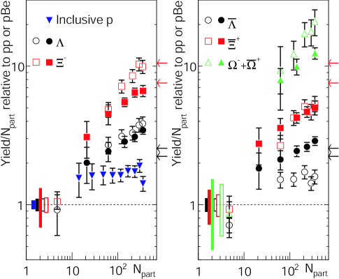
Figure 14: Enhanced strange baryon production as a function of $\left\langle N_{part}\right\rangle$, at mid-rapidity, in $AA$ collisions compared to $\left\langle N_{part}\right\rangle$-scaled $pp$ interactions at the same energy. Solid markers: STAR data on AuAu collisions at $\sqrt{s_{NN}}=200$ GeV. Open symbols: SPS data on PbPb collisions at $\sqrt{s_{NN}}=17.3$ GeV. Boxes at unity show statistical and systematic uncertainties and arrows on the right axes mark the predictions of a thermal model. Figure from [71].

For a review of strange hadron production in heavy-ion collisions from SPS to RHIC, see [72]. For the ALICE (LHC) results on multi-strange baryon production at 2.76 TeV, see [73]. ALICE observed that the strangeness enhancement was less pronounced than at lower energies.

3.4 Sequential melting of heavy quarkonia

Colour Debye screening of the attraction between heavy quarks ($c$ or $b$) and antiquarks ($\bar{c}$ or $\bar{b}$) in a hot and dense medium such as QGP is expected to suppress the formation of quarkonia relative to what one expects from a $pp$ baseline measurement [74]. Observation of suppression would thus serve as a signal for deconfinement. As the temperature of the medium rises, various quarkonium states are expected to ‘melt’ one by one in the sequence of their increasing binding energies. The sequential melting of heavy quarkonia thus serves as a ‘thermometer’ for the medium. A reliable estimation of the charmonium formation rates, however, needs to take into account several other competing effects:

• gluon shadowing/anti-shadowing and saturation effects in the initial wave functions of the colliding nuclei,

• initial- and final-state $k_{T}$ scatterings and parton-energy loss,

• charmonium formation via colour-singlet and colour-octet channels,

• feed-down from the excited states of the charmonium to its ground state,

• secondary charmonium production by recombination or coalescence of independently produced $c$ and $\bar{c}$,

• interaction of the outgoing charmonium with the medium, etc.

A systematic study of suppression patterns of $J/\psi$ and $\Upsilon$ families, together with $pA$ baseline measurements, over a broad energy range, would help disentangle these hot and cold nuclear matter effects.

For reviews of charmonium and/or bottomonium production in heavy-ion collisions, see [75, 76, 77, 78]. For a review of heavy-flavour probes of the QCD matter formed at RHIC, see [79].

4 Big Bang and Little Bang

Having described the various stages in the relativistic heavy-ion collisions and the most important observables and probes in this field, let me bring out the striking similarities between the Big Bang and the Little Bang. In both cosmology and the physics of relativistic heavy-ion collisions, the initial quantum fluctuations ultimately lead to macroscopic fluctuations and anisotropies in the final state. In both the fields, the goal is to learn about the early state of the matter from the final-state observations. See Table 1 for the comparison of these two fields. Here 2.73 K and 1.95 K are photon and neutrino decoupling or freezeout temperatures, respectively. $T_{ch}$ and $T_{kin}$ are the chemical and kinetic freezeout temperatures mentioned in section 1. The last two rows list the various experimental ‘tools’ and the years in which they were commissioned. For a more detailed comparison, see [5, 80, 81].

Table 1: Big Bang and Little Bang comparison

	Big Bang	Little Bang
Occurrence	Only once	Millions of times at RHIC, LHC
Initial state	Inflation? ($10^{-35}$ s)	Glasma? ($10^{-24}$ s)
Expansion	General Relativity	Rel. imperfect fluid dynamics
Freezeout temperatures	$\gamma:2.73$ K, $\nu:1.95$ K	$T_{ch}\sim 150,T_{kin}\sim 120$ MeV
Anisotropy in	Final temp. (CMB)	Final flow profile
Penetrating probes	Photons	Photons, jets
Chemical probes	Light nuclei	Various hadron species
Colour shift	Red shift	Blue shift
Tools	COBE, WMAP, Planck	SPS, RHIC, LHC
Starting years	1989, 2001, 2009	1987, 2000, 2009

5 Fluid dynamics

The kinetic or transport theory of gases is a microscopic description in the sense that detailed knowledge of the motion of the constituents is required. Fluid dynamics (also loosely called hydrodynamics) is an effective (macroscopic) theory that describes the slow, long-wavelength motion of a fluid close to local thermal equilibrium. No knowledge of the motion of the constituents is required to describe observable phenomena. Quantitatively, if $l$ denotes the mean free path, $\tau$ the mean free time, $k$ the wave number, and $\omega$ the frequency, then $kl\ll 1,~{}\omega\tau\ll 1$ is the hydrodynamic regime, $kl\simeq 1,~{}\omega\tau\simeq 1$ the kinetic regime, and $kl\gg 1,~{}\omega\tau\gg 1$ the nearly-free-particle regime.

Relativistic hydrodynamic equations are a set of coupled partial differential equations for number density $n$, energy density $\epsilon$, pressure $P$, hydrodynamic four-velocity $u^{\mu}$, and in the case of imperfect hydrodynamics, also bulk viscous pressure $\Pi$, particle-diffusion current $n^{\mu}$, and shear stress tensor $\pi^{\mu\nu}$. In addition, these equations also contain the coefficients of shear and bulk viscosities and thermal conductivity, and the corresponding relaxation times. Further, the equation of state (EoS) needs to be supplied to make the set of equations complete. Hydrodynamics is a powerful technique: Given the initial conditions and the EoS, it predicts the evolution of the matter. Its limitation is that it is applicable at or near (local) thermal equilibrium only.

Relativistic hydrodynamics finds applications in cosmology, astrophysics, high-energy nuclear physics, etc. In relativistic heavy-ion collisions, it is used to calculate the multiplicity and transverse momentum spectra of hadrons, anisotropic flows, and femtoscopic radii. Energy density or temperature profiles resulting from the hydrodynamic evolution are needed in the calculations of jet quenching, $J/\psi$ melting, thermal photon and dilepton productions, etc. Thus hydrodynamics plays a central role in modeling relativistic heavy-ion collisions.

Hydrodynamics is formulated as an order-by-order expansion in the sense that in the first (second)-order theory, the equations for the dissipative fluxes contain the first (second) derivatives of $u^{\mu}$. The ideal hydrodynamics is called the zeroth-order theory. The zeroth-, first-, and second-order equations are named after Euler, Navier-Stokes, and Burnett, respectively, in the non-relativistic case (Fig. 15). The relativistic Navier-Stokes equations are parabolic in nature and exhibit acausal behaviour, which was rectified in the (relativistic second-order) Israel-Stewart (IS) theory [29]. The formulation of the relativistic imperfect second-order hydrodynamics (‘2’ in Fig. 15) is currently under intense investigation; see, e.g., [82, 83, 84, 85, 86] for the recent activity in this area. Hydrodynamics has traditionally been derived either from entropy considerations (i.e., the generalized second law of thermodynamics) or by taking the second moment of the Boltzmann equation.

Figure 15: Coarse-Graining of the Boltzmann equation

For a comprehensive treatment of relativistic hydrodynamics, numerical techniques, and applications, see [87]. For an elementary introduction to relativistic hydrodynamics and its application to heavy-ion collisions, see [88]. For a review of new developments in relativistic viscous hydrodynamics, see [89].

6 LHC highlights

6.1 RHIC-LHC comparison

Table 2 compares some basic results obtained at LHC soon after it started operating, with similar results obtained earlier at RHIC. Here $dN_{ch}/d\eta$ is the charged particle pseudorapidity density, at mid-rapidity, normalized by $\left\langle N_{part}\right\rangle/2$ where $\left\langle N_{part}\right\rangle$ is the mean number of participating nucleons in a nucleus-nucleus collision, estimated using the Glauber model [25]. $\epsilon_{Bj}$ is the initial energy density estimated using the well-known Bjorken formula [5, 7]. $\tau_{i}$ is the initial or formation time of QGP. Assuming conservatively the same $\tau_{i}\simeq 0.5$ fm at LHC as at RHIC, one gets an estimate of $\epsilon_{Bj}$ at LHC. $T_{i}$ is the initial temperature fitted to reproduce the observed multiplicity of charged particles in a hydrodynamical model. Note that the $\sim 30$% increase in $T_{i}$ is consistent with the factor of $\sim 3$ rise in $\epsilon_{Bj}$. $V_{f.o.}$ is the volume of the system at the freezeout, measured with two-pion Bose-Einstein correlations. $v_{flow}$ is the radial velocity of the collective flow of matter. $v_{2}$ is the elliptic flow. It is clear from Table 2 that the QGP fireball produced at LHC is hotter, larger, and longer-lasting, as compared with that at RHIC.

Table 2: RHIC-LHC comparison

	RHIC (AuAu)	LHC (PbPb)	Increase by factor or %
$\sqrt{s_{NN}}$ (GeV)	200	2760	14
$dN_{ch}/d\eta/\left(\frac{<N_{part}>}{2}\right)$	3.76	8.4	2.2
$\epsilon_{Bj}\tau_{i}$ (GeV/fm2)	16/3	16	3
$\epsilon_{Bj}$ (GeV/fm3)	10	30	3
$T_{i}$ (MeV)	360	470	30%
$V_{f.o.}$ (fm3)	2500	5000	2
Lifetime (fm$/c$)	8.4	10.6	26%
$v_{flow}$	0.6	0.66	10%
$<p_{T}>_{\pi}$ (GeV)	0.36	0.45	25%
Differential $v_{2}(p_{T})$			unchanged
$p_{T}$-integrated $v_{2}$			30%

6.2 Some surprises at LHC

6.2.1 Charged-particle production at LHC

Figure 16 presents perhaps the most basic observable in heavy-ion collisions — the number of charged particles produced. This observable helps place constraints on the particle production mechanisms and provides a first rough estimate of the initial energy density reached in the collision. The left panel compares the charged-particle production in central $AA$ and non-single-diffractive (NSD) $pp(p\bar{p})$ collisions at various energies and facilities. The curves are simple parametric fits to the data; note the higher power of $s_{NN}$ in the former case. The precise magnitude of $dN_{ch}/d\eta$ measured in PbPb collisions at LHC was somewhat on a higher side than expected. Indeed, as is clear from the figure, the logarithmic extrapolation of the lower-energy measurements at AGS, SPS, and RHIC grossly under-predicts the LHC data. The right panel highlights an even more surprising fact that the shape of the plotted observable vs centrality is nearly independent of the centre-of-mass energy, except perhaps for the most peripheral $AA$ collisions. Studying the centrality dependence of the charged-particle production throws light on the roles played by hard scatterings and soft processes. For details, see [91].

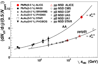
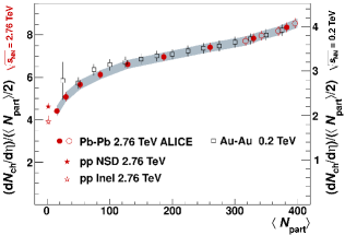
Figure 16: Charged-particle pseudorapidity density (at $\eta=0$) per colliding nucleon pair vs $\sqrt{s_{NN}}$ (left panel) and $\left\langle N_{part}\right\rangle$ (right panel). Figure from [90].

6.2.2 Particle ratios at LHC — Proton anomaly

We described above in section 3.2 the success of the thermal/statistical hadronization model in explaining the ratios of particle abundances measured at AGS, SPS, and RHIC. When extended to the LHC energies, however, the model was unable to reproduce the $p/\pi^{+}$ and $\bar{p}/\pi^{-}$ ratios; the absolute $p,\bar{p}$ yields were off by almost three standard deviations (Fig. 17). Current attempts to understand these discrepancies focus on the possible effects of (a) as yet undiscovered hadrons, or in other words, the incomplete hadron spectrum, (b) the annihilation of some $p,\bar{p}$ in the final hadronic phase, or (c) the out-of-equilibrium physics currently missing in the model. None of these effects has been found to be satisfactory because while reducing the (Data-Fit) discrepancy at one place, it worsens it at other place(s) [92]. Finally, Fig. 17 also shows that most antiparticle/particle ratios are unity within error bars indicating a vanishing baryo-chemical potential at LHC.

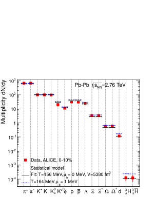
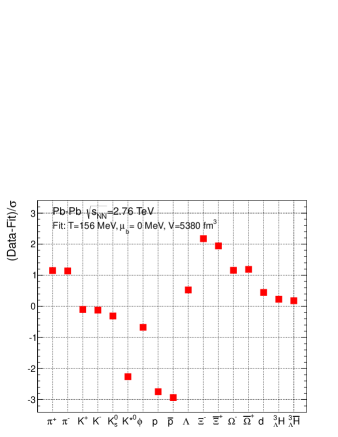
Figure 17: Left: Hadron yields from ALICE (LHC) together with the fit based on the thermal model (solid black lines). The data point for $K^{0*}$ is not included in the fit. Blue dotted lines show results of the model for the indicated values of $T$ and $\mu_{b}$, normalized to the value for $\pi^{+}$. Right: Deviations between the thermal fit and the data. Note that the $p$ and $\bar{p}$ yields are below the thermal fit by 2.7 and 2.9 sigma, respectively, whereas the cascade yields are above the fit by about two sigma. Figures from [92].

6.2.3 Quarkonium story at LHC

We described above in section 3.4 the melting of heavy quarkonium as a possible signature of deconfinement or colour screening effects in QGP. Anomalous suppression of $J/\psi$ was first seen at SPS. No significant differences in the suppression pattern were observed at RHIC. LHC, however, has thrown some surprises which are not yet fully understood. Figure 18 presents the nuclear modification factor $R_{AA}$ of $J/\psi$ as a function of centrality (left) and $p_{T}$ (right), at similar rapidities. Note the differences between the PHENIX and ALICE measurements. Differences at low $p_{T}$ in the right-hand panel are possibly because of the larger recombination probability at ALICE than at PHENIX; this probability is expected to decrease at high $p_{T}$. Sequential suppression of upsilon states was observed by CMS in PbPb collisions at 2.76 TeV: The $R_{AA}$ values for $\Upsilon$(1S), $\Upsilon$(2S), and $\Upsilon$(3S), were about 0.56, 0.12, and lower than 0.10, respectively [94]. For the status of the evolving quarkonium saga, see [95].

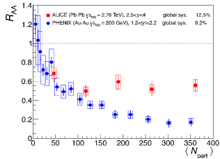
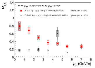
Figure 18: Nuclear modification factor $R_{AA}$ of $J/\psi$ vs centrality (left) and $p_{T}$ (right). Figures from [90] and [93].

7 Concluding remarks

(1) Quark-gluon plasma has been discovered, and we are in the midst of trying to determine its thermodynamic and transport properties accurately.

(2) Data on the collective flow at RHIC/LHC have provided a strong support to hydrodynamics as the appropriate effective theory for relativistic heavy-ion collisions. The most complete event-to-event hydrodynamic calculations to date [96, 43] have yielded $\eta/s=0.12$ and 0.20 at RHIC (AuAu, 200 GeV) and LHC (PbPb, 2.76 TeV), respectively, with at least 50% systematic uncertainties. These are the average values over the temperature histories of the collisions. Uncertainties associated with (mainly) the initial conditions have so far prevented a more precise determination of $\eta/s$.

(3) Surprisingly, even the $pp$ collision data at 7 TeV are consistent with the hydrodynamic picture, if the final multiplicity is sufficiently large!

(4) An important open question is at what kinematic scale partons lose their quasiparticle nature (evident in jet quenching) and become fluid like (as seen in the collective flow)?

(5) QCD phase diagram still remains largely unknown.

(6) RHIC remains operational. ALICE, ATLAS, and CMS at LHC all have come up with many new results on heavy-ion collisions. Further updates of these facilities are planned or being proposed. Compressed baryonic matter experiments at FAIR [10] and NICA [97], which will probe the QCD phase diagram in a high baryon density but relatively low temperature region, are a few years in the future. Electron-ion collider (EIC) has been proposed to understand the glue that binds us all [98]. So this exciting field is going to remain very active for a decade at least.

Many review articles have been cited throughout the text above. Here are a few more published in the last 2-3 years [99, 100]. See also these two talks given at the ‘2013 Nobel Symposium on LHC Physics’ for an overview of the status of this field: [101, 102].

References

- [1] H. Satz, Extreme States of Matter in Strong Interaction Physics, Lect. Notes in Phys. 841 (2012) 1, (Springer, Heidelberg, 2012).
- [2] W. Florkowski, Phenomenology of Ultra-relativistic Heavy-Ion Collisions, (World Scientific, Singapore, 2010).
- [3] J. Bartke, Relativistic Heavy-Ion Physics, (World Scientific, Singapore, 2008).
- [4] R. Vogt, Ultra-relativistic Heavy-Ion Collisions, (Elsevier Science, Amsterdam, 2007).
- [5] K. Yagi, T. Hatsuda, and Y. Miake, Quark-Gluon Plasma, (Cambridge University Press, Cambridge, 2005).
- [6] J. Letessier and J. Rafelski, Hadrons and Quark-Gluon Plasma, (Cambridge University Press, Cambridge, 2002).
- [7] C.Y. Wong, Introduction to High-Energy Heavy-Ion Collisions, (World Scientific, Singapore, 1994).
- [8] L. Csernai, Introduction to Relativistic Heavy-Ion Collisions, (John Wiley, 1994).
- [9] B. Müller, The Physics of the Quark-Gluon Plasma, Lect. Notes in Phys. 225 (1985) 1, (Springer, Heidelberg, 1985).
- [10] B. Friman, C. Hohne, J. Knoll, S. Leupold, J. Randrup, R. Rapp, and P. Senger, (eds.), The CBM physics book: Compressed baryonic matter in laboratory experiments, Lect. Notes in Phys. 814 (2011) 1, (Springer, Heidelberg, 2011).
- [11] R.C. Hwa and X.N. Wong, (eds.), Quark-Gluon Plasma, Vols. 3, 4, (World Scientific, Singapore, 2004, 2010).
- [12] R.C. Hwa, (ed.), Quark-Gluon Plasma, Vols. 1, 2, (World Scientific, Singapore, 1990, 1995).
- [13] Illustration by Pete Harrison, Langlo Press, reproduced with permission.
- [14] S. Borsanyi et al., JHEP 1011 (2010) 077.
- [15] S. Borsanyi et al., arXiv:1309.5258 [hep-lat].
- [16] K. Rajagopal and F. Wilczek, in M. Shifman (ed.): At the frontier of particle physics, vol. 3, 2061-2151.
- [17] M. G. Alford, A. Schmitt, K. Rajagopal, and T. Schaefer, Rev. Mod. Phys. 80 (2008) 1455.
- [18] R. Anglani et al., arXiv:1302.4264 [hep-ph].
- [19] L. McLerran and R. D. Pisarski, Nucl. Phys. A 796 (2007) 83.
- [20] J. Adams et al. [STAR Collaboration], Nucl. Phys. A 757 (2005) 102.
- [21] K. Rajagopal, Nucl. Phys. A 661 (1999) 150.
- [22] P. Petreczky, J. Phys. G 39 (2012) 093002.
- [23] J. D. Bjorken, Lect. Notes Phys. 56 (1976) 93.
- [24] F. Gelis, E. Iancu, J. Jalilian-Marian, and R. Venugopalan, Ann. Rev. Nucl. Part. Sci. 60 (2010) 463.
- [25] M. L. Miller, K. Reygers, S. J. Sanders, and P. Steinberg, Ann. Rev. Nucl. Part. Sci. 57 (2007) 205.
- [26] D. Kharzeev and M. Nardi, Phys. Lett. B 507 (2001) 121.
- [27] J. L. Albacete and C. Marquet, arXiv:1401.4866 [hep-ph].
- [28] I. Muller, Z. Phys. 198 (1967) 329.
- [29] W. Israel and J. M. Stewart, Annals Phys. 118 (1979) 341.
- [30] P. Huovinen and P. Petreczky, Nucl. Phys. A 837 (2010) 26.
- [31] H. Song, S. A. Bass, U. Heinz, T. Hirano, and C. Shen, Phys. Rev. C 83 (2011) 054910 [Erratum-ibid. C 86 (2012) 059903].
- [32] M. Gyulassy and L. McLerran, Nucl. Phys. A 750 (2005) 30.
- [33] R. A. Lacey et al., Phys. Rev. Lett. 98 (2007) 092301.
- [34] T. Schaefer and D. Teaney, Rept. Prog. Phys. 72 (2009) 126001.
- [35] L. P. Csernai, J. .I. Kapusta, and L. D. McLerran, Phys. Rev. Lett. 97 (2006) 152303.
- [36] S. Voloshin and Y. Zhang, Z. Phys. C 70 (1996) 665.
- [37] A. M. Poskanzer and S. A. Voloshin, Phys. Rev. C 58 (1998) 1671.
- [38] S. A. Voloshin, A. M. Poskanzer, and R. Snellings, arXiv:0809.2949 [nucl-ex].
- [39] M. D. Oldenburg [STAR Collaboration], J. Phys. G 31 (2005) S437.
- [40] B. Alver et al., Phys. Rev. C 77 (2008) 014906.
- [41] D. Teaney and L. Yan, Phys. Rev. C 83 (2011) 064904.
- [42] U. Heinz and R. Snellings, Ann. Rev. Nucl. Part. Sci. 63 (2013) 123.
- [43] C. Gale, S. Jeon, and B. Schenke, Int. J. Mod. Phys. A 28 (2013) 1340011.
- [44] P. Huovinen, Int. J. Mod. Phys. E 22 (2013) 1330029.
- [45] D. d’Enterria, arXiv:0902.2011 [nucl-ex].
- [46] I. Vitev and M. Gyulassy, Phys. Rev. Lett. 89 (2002) 252301.
- [47] I. Vitev, J. Phys. G 30 (2004) S791.
- [48] S. S. Adler et al. [PHENIX Collaboration], Phys. Rev. C 75 (2007) 024909.
- [49] B. Abelev et al. [ALICE Collaboration], Phys. Rev. Lett. 110 (2013) 082302.
- [50] J. Adams et al. [STAR Collaboration], Phys. Rev. Lett. 91 (2003) 072304.
- [51] J. Adams et al. [STAR Collaboration], Phys. Rev. Lett. 95 (2005) 152301.
- [52] S. Chatrchyan et al. [CMS Collaboration], Phys. Rev. C 84 (2011) 024906.
- [53] U. A. Wiedemann, arXiv:0908.2306 [hep-ph].
- [54] A. Majumder and M. Van Leeuwen, Prog. Part. Nucl. Phys. A 66 (2011) 41.
- [55] M. Spousta, Mod. Phys. Lett. A 28 (2013) 1330017.
- [56] B. Tomasik and U. A. Wiedemann, In *Hwa, R.C. (ed.) et al.: Quark gluon plasma* 715-777 [hep-ph/0210250].
- [57] S. S. Padula, Braz. J. Phys. 35 (2005) 70.
- [58] M. A. Lisa, S. Pratt, R. Soltz, and U. Wiedemann, Ann. Rev. Nucl. Part. Sci. 55 (2005) 357.
- [59] G. David, R. Rapp, and Z. Xu, Phys. Rept. 462 (2008) 176.
- [60] I. Tserruya, arXiv:0903.0415 [nucl-ex].
- [61] B. Müller, Acta Phys. Polon. B 38 (2007) 3705.
- [62] F. Noferini [ALICE Collaboration], Nucl. Phys. A 904-905 (2013) 483c.
- [63] R. J. Fries, V. Greco, and P. Sorensen, Ann. Rev. Nucl. Part. Sci. 58 (2008) 177.
- [64] P. Braun-Munzinger, K. Redlich, and J. Stachel, In *Hwa, R.C. (ed.) et al.: Quark gluon plasma* 491-599 [nucl-th/0304013].
- [65] F. Becattini, arXiv:0901.3643 [hep-ph].
- [66] J. Cleymans and K. Redlich, Phys. Rev. Lett. 81 (1998) 5284. [nucl-th/9808030].
- [67] A. Andronic, P. Braun-Munzinger, and J. Stachel, Phys. Lett. B 673 (2009) 142 [Erratum-ibid. B 678 (2009) 516].
- [68] P. Braun-Munzinger and J. Stachel, arXiv:0901.2500 [nucl-th].
- [69] J. Rafelski and B. Müller, Phys. Rev. Lett. 48 (1982) 1066 [Erratum-ibid. 56 (1986) 2334].
- [70] P. Koch, B. Müller, and J. Rafelski, Phys. Rept. 142 (1986) 167.
- [71] B. I. Abelev et al. [STAR Collaboration], Phys. Rev. C 77 (2008) 044908.
- [72] C. Blume and C. Markert, Prog. Part. Nucl. Phys. 66 (2011) 834.
- [73] B. B. Abelev et al. [ALICE Collaboration], Phys. Lett. B 728 (2014) 216.
- [74] T. Matsui and H. Satz, Phys. Lett. B 178 (1986) 416.
- [75] L. Kluberg and H. Satz, arXiv:0901.3831 [hep-ph].
- [76] O. Linnyk, E. L. Bratkovskaya, and W. Cassing, Int. J. Mod. Phys. E 17 (2008) 1367.
- [77] R. Rapp, D. Blaschke, and P. Crochet, Prog. Part. Nucl. Phys. 65 (2010) 209.
- [78] N. Brambilla, et al., Eur. Phys. J. C 71 (2011) 1534.
- [79] A. D. Frawley, T. Ullrich, and R. Vogt, Phys. Rept. 462 (2008) 125.
- [80] A. P. Mishra, R. K. Mohapatra, P. S. Saumia, and A. M. Srivastava, Phys. Rev. C 77 (2008) 064902.
- [81] A. P. Mishra, R. K. Mohapatra, P. S. Saumia, and A. M. Srivastava, Phys. Rev. C 81 (2010) 034903.
- [82] G. S. Denicol, H. Niemi, E. Molnar, and D. H. Rischke, Phys. Rev. D 85 (2012) 114047.
- [83] G. S. Denicol, E. Molnár, H. Niemi, and D. H. Rischke, Eur. Phys. J. A 48 (2012) 170.
- [84] A. Jaiswal, R. S. Bhalerao, and S. Pal, Phys. Rev. C 87 (2013) 021901 (R).
- [85] A. Jaiswal, R. S. Bhalerao, and S. Pal, Phys. Lett. B 720 (2013) 347.
- [86] R. S. Bhalerao, A. Jaiswal, S. Pal, and V. Sreekanth, arXiv:1312.1864 [nucl-th].
- [87] L. Rezzolla and O. Zanotti, Relativistic Hydrodynamics, (Oxford University Press, Oxford, 2013).
- [88] J. -Y. Ollitrault, Eur. J. Phys. 29 (2008) 275.
- [89] P. Romatschke, Int. J. Mod. Phys. E 19 (2010) 1.
- [90] K. Reygers [ALICE Collaboration], arXiv:1208.1626 [nucl-ex].
- [91] E. Abbas et al. [ALICE Collaboration], Phys. Lett. B 726 (2013) 610.
- [92] J. Stachel, A. Andronic, P. Braun-Munzinger, and K. Redlich, arXiv:1311.4662 [nucl-th].
- [93] B. B. Abelev et al. [ALICE Collaboration], arXiv:1311.0214 [nucl-ex].
- [94] S. Chatrchyan et al. [CMS Collaboration], Phys. Rev. Lett. 109 (2012) 222301.
- [95] I. Tserruya, arXiv:1311.4456 [nucl-ex].
- [96] C. Gale, S. Jeon, B. Schenke, P. Tribedy and R. Venugopalan, Phys. Rev. Lett. 110 (2013) 012302.
- [97] V. D. Kekelidze et al. [NICA and MPD Collaborations], Phys. Atom. Nucl. 75 (2012) 542.
- [98] A. Accardi et al., arXiv:1212.1701 [nucl-ex].
- [99] B. Müller, J. Schukraft, and B. Wyslouch, Ann. Rev. Nucl. Part. Sci. 62, 361 (2012).
- [100] B. V. Jacak and B. Müller, Science 337, 310 (2012).
- [101] B. Müller, arXiv:1309.7616 [nucl-th].
- [102] J. Schukraft, arXiv:1311.1429 [hep-ex].