I Introduction
Top quark plays a special role in the standard model(SM) and holds
great promise in revealing the secret of new physics beyond the SM.
The running LHC is a top-quark factory, and provides a great
opportunity to seek out top-quark rare decays. Among those rare
processes, the flavor-changing neutral current (FCNC) decays
t → c h → 𝑡 𝑐 ℎ t\rightarrow ch m h 0 ∼ 124 − 126 GeV similar-to subscript 𝑚 subscript ℎ 0 124 126 GeV m_{h_{0}}\sim 124-126\;{\rm GeV} ref1 ; ref2
In the framework of the SM, the possibility of detecting FCNC decays
t → c h → 𝑡 𝑐 ℎ t\rightarrow ch ref201 ; ref202 ref3 ; ref4 ref5 10 − 13 superscript 10 13 10^{-13} ref6 t → c h → 𝑡 𝑐 ℎ t\rightarrow ch ( t → c h ) S U S Y − E W ∼ 10 − 8 {}^{SUSY-EW}(t\rightarrow ch)\sim 10^{-8} ( t → c h ) S U S Y − Q C D ∼ 10 − 5 {}^{SUSY-QCD}(t\rightarrow ch)\sim 10^{-5} ref61 tan β = 1.5 o r 35 𝛽 1.5 𝑜 𝑟 35 \tan\beta=1.5\ or\ 35 t → c h → 𝑡 𝑐 ℎ t\rightarrow ch 3 × 10 − 6 3 superscript 10 6 3\times 10^{-6}
Physicists have been interested in the MSSM
ref7 ; ref71 ; ref72 ; ref73 ref8 ; ref81 ref9 ; ref10
In BLMSSM, B and L are spontaneously broken near the weak scale, the proton decay is forbidden, and the three neutrinos get mass from the extended seesaw mechanism at tree levelref201 ; ref202 ; ref9 ; ref10
The CMSref1001 ref1002 ref9 ; ref10 ; ref1003 ref201 ; ref202 ; ref1004 ref1005
In this paper we analyze the corrections to the top-quark decay
t → c h → 𝑡 𝑐 ℎ t\rightarrow ch t → c h → 𝑡 𝑐 ℎ t\rightarrow ch
II A supersymmtric extension of the SM where B and L are local gauge symmetries
The local gauge B and L is base on the gauge group:
S U ( 3 ) C ⊗ S U ( 2 ) L ⊗ U ( 1 ) Y ⊗ U ( 1 ) B ⊗ U ( 1 ) L tensor-product tensor-product tensor-product tensor-product 𝑆 𝑈 subscript 3 𝐶 𝑆 𝑈 subscript 2 𝐿 𝑈 subscript 1 𝑌 𝑈 subscript 1 𝐵 𝑈 subscript 1 𝐿 SU(3)_{{}_{C}}\otimes SU(2)_{{}_{L}}\otimes U(1)_{{}_{Y}}\otimes U(1)_{{}_{B}}\otimes U(1)_{{}_{L}} B 𝐵 B L 𝐿 L Q ^ 4 subscript ^ 𝑄 4 \hat{Q}_{{}_{4}} U ^ 4 c superscript subscript ^ 𝑈 4 𝑐 \hat{U}_{{}_{4}}^{c} D ^ 4 c superscript subscript ^ 𝐷 4 𝑐 \hat{D}_{{}_{4}}^{c} Q ^ 5 c superscript subscript ^ 𝑄 5 𝑐 \hat{Q}_{{}_{5}}^{c} U ^ 5 subscript ^ 𝑈 5 \hat{U}_{{}_{5}} D ^ 5 subscript ^ 𝐷 5 \hat{D}_{{}_{5}} L ^ 4 subscript ^ 𝐿 4 \hat{L}_{{}_{4}} E ^ 4 c superscript subscript ^ 𝐸 4 𝑐 \hat{E}_{{}_{4}}^{c} N ^ 4 c superscript subscript ^ 𝑁 4 𝑐 \hat{N}_{{}_{4}}^{c} L ^ 5 c superscript subscript ^ 𝐿 5 𝑐 \hat{L}_{{}_{5}}^{c} E ^ 5 subscript ^ 𝐸 5 \hat{E}_{{}_{5}} N ^ 5 subscript ^ 𝑁 5 \hat{N}_{{}_{5}} Φ ^ B subscript ^ Φ 𝐵 \hat{\Phi}_{{}_{B}} φ ^ B subscript ^ 𝜑 𝐵 \hat{\varphi}_{{}_{B}} Φ ^ L subscript ^ Φ 𝐿 \hat{\Phi}_{{}_{L}} φ ^ L subscript ^ 𝜑 𝐿 \hat{\varphi}_{{}_{L}} X ^ ^ 𝑋 \hat{X} X ^ ′ superscript ^ 𝑋 ′ \hat{X}^{\prime}
Table 1: The properties of superfields in BLMSSM
In BLMSSM, the super potential is written as ref11 ; ref12
𝒲 B L M S S M = 𝒲 M S S M + 𝒲 B + 𝒲 L + 𝒲 X , subscript 𝒲 𝐵 𝐿 𝑀 𝑆 𝑆 𝑀 subscript 𝒲 𝑀 𝑆 𝑆 𝑀 subscript 𝒲 𝐵 subscript 𝒲 𝐿 subscript 𝒲 𝑋 \displaystyle{\cal W}_{{}_{BLMSSM}}={\cal W}_{{}_{MSSM}}+{\cal W}_{{}_{B}}+{\cal W}_{{}_{L}}+{\cal W}_{{}_{X}}\;, (1)
where 𝒲 M S S M subscript 𝒲 𝑀 𝑆 𝑆 𝑀 {\cal W}_{{}_{MSSM}} 𝒲 B subscript 𝒲 𝐵 {\cal W}_{{}_{B}} 𝒲 L subscript 𝒲 𝐿 {\cal W}_{{}_{L}} 𝒲 X subscript 𝒲 𝑋 {\cal W}_{{}_{X}}
𝒲 B = λ Q Q ^ 4 Q ^ 5 c Φ ^ B + λ U U ^ 4 c U ^ 5 φ ^ B + λ D D ^ 4 c D ^ 5 φ ^ B + μ B Φ ^ B φ ^ B subscript 𝒲 𝐵 subscript 𝜆 𝑄 subscript ^ 𝑄 4 superscript subscript ^ 𝑄 5 𝑐 subscript ^ Φ 𝐵 subscript 𝜆 𝑈 superscript subscript ^ 𝑈 4 𝑐 subscript ^ 𝑈 5 subscript ^ 𝜑 𝐵 subscript 𝜆 𝐷 superscript subscript ^ 𝐷 4 𝑐 subscript ^ 𝐷 5 subscript ^ 𝜑 𝐵 subscript 𝜇 𝐵 subscript ^ Φ 𝐵 subscript ^ 𝜑 𝐵 \displaystyle{\cal W}_{{}_{B}}=\lambda_{{}_{Q}}\hat{Q}_{{}_{4}}\hat{Q}_{{}_{5}}^{c}\hat{\Phi}_{{}_{B}}+\lambda_{{}_{U}}\hat{U}_{{}_{4}}^{c}\hat{U}_{{}_{5}}\hat{\varphi}_{{}_{B}}+\lambda_{{}_{D}}\hat{D}_{{}_{4}}^{c}\hat{D}_{{}_{5}}\hat{\varphi}_{{}_{B}}+\mu_{{}_{B}}\hat{\Phi}_{{}_{B}}\hat{\varphi}_{{}_{B}}
+ Y u 4 Q ^ 4 H ^ u U ^ 4 c + Y d 4 Q ^ 4 H ^ d D ^ 4 c + Y u 5 Q ^ 5 c H ^ d U ^ 5 + Y d 5 Q ^ 5 c H ^ u D ^ 5 , subscript 𝑌 subscript 𝑢 4 subscript ^ 𝑄 4 subscript ^ 𝐻 𝑢 superscript subscript ^ 𝑈 4 𝑐 subscript 𝑌 subscript 𝑑 4 subscript ^ 𝑄 4 subscript ^ 𝐻 𝑑 superscript subscript ^ 𝐷 4 𝑐 subscript 𝑌 subscript 𝑢 5 superscript subscript ^ 𝑄 5 𝑐 subscript ^ 𝐻 𝑑 subscript ^ 𝑈 5 subscript 𝑌 subscript 𝑑 5 superscript subscript ^ 𝑄 5 𝑐 subscript ^ 𝐻 𝑢 subscript ^ 𝐷 5 \displaystyle\hskip 34.14322pt+Y_{{}_{u_{4}}}\hat{Q}_{{}_{4}}\hat{H}_{{}_{u}}\hat{U}_{{}_{4}}^{c}+Y_{{}_{d_{4}}}\hat{Q}_{{}_{4}}\hat{H}_{{}_{d}}\hat{D}_{{}_{4}}^{c}+Y_{{}_{u_{5}}}\hat{Q}_{{}_{5}}^{c}\hat{H}_{{}_{d}}\hat{U}_{{}_{5}}+Y_{{}_{d_{5}}}\hat{Q}_{{}_{5}}^{c}\hat{H}_{{}_{u}}\hat{D}_{{}_{5}}\;,
𝒲 L = Y e 4 L ^ 4 H ^ d E ^ 4 c + Y ν 4 L ^ 4 H ^ u ν ^ 4 c + Y e 5 L ^ 5 c H ^ u E ^ 5 + Y ν 5 L ^ 5 c H ^ d ν ^ 5 subscript 𝒲 𝐿 subscript 𝑌 subscript 𝑒 4 subscript ^ 𝐿 4 subscript ^ 𝐻 𝑑 superscript subscript ^ 𝐸 4 𝑐 subscript 𝑌 subscript 𝜈 4 subscript ^ 𝐿 4 subscript ^ 𝐻 𝑢 superscript subscript ^ 𝜈 4 𝑐 subscript 𝑌 subscript 𝑒 5 superscript subscript ^ 𝐿 5 𝑐 subscript ^ 𝐻 𝑢 subscript ^ 𝐸 5 subscript 𝑌 subscript 𝜈 5 superscript subscript ^ 𝐿 5 𝑐 subscript ^ 𝐻 𝑑 subscript ^ 𝜈 5 \displaystyle{\cal W}_{{}_{L}}=Y_{{}_{e_{4}}}\hat{L}_{{}_{4}}\hat{H}_{{}_{d}}\hat{E}_{{}_{4}}^{c}+Y_{{}_{\nu_{4}}}\hat{L}_{{}_{4}}\hat{H}_{{}_{u}}\hat{\nu}_{{}_{4}}^{c}+Y_{{}_{e_{5}}}\hat{L}_{{}_{5}}^{c}\hat{H}_{{}_{u}}\hat{E}_{{}_{5}}+Y_{{}_{\nu_{5}}}\hat{L}_{{}_{5}}^{c}\hat{H}_{{}_{d}}\hat{\nu}_{{}_{5}}
+ Y ν L ^ H ^ u ν ^ c + λ ν c ν ^ c ν ^ c φ ^ L + μ L Φ ^ L φ ^ L , subscript 𝑌 𝜈 ^ 𝐿 subscript ^ 𝐻 𝑢 superscript ^ 𝜈 𝑐 subscript 𝜆 superscript 𝜈 𝑐 superscript ^ 𝜈 𝑐 superscript ^ 𝜈 𝑐 subscript ^ 𝜑 𝐿 subscript 𝜇 𝐿 subscript ^ Φ 𝐿 subscript ^ 𝜑 𝐿 \displaystyle\hskip 34.14322pt+Y_{{}_{\nu}}\hat{L}\hat{H}_{{}_{u}}\hat{\nu}^{c}+\lambda_{{}_{\nu^{c}}}\hat{\nu}^{c}\hat{\nu}^{c}\hat{\varphi}_{{}_{L}}+\mu_{{}_{L}}\hat{\Phi}_{{}_{L}}\hat{\varphi}_{{}_{L}}\;,
𝒲 X = λ 1 Q ^ Q ^ 5 c X ^ + λ 2 U ^ c U ^ 5 X ^ ′ + λ 3 D ^ c D ^ 5 X ^ ′ + μ X X ^ X ^ ′ , subscript 𝒲 𝑋 subscript 𝜆 1 ^ 𝑄 superscript subscript ^ 𝑄 5 𝑐 ^ 𝑋 subscript 𝜆 2 superscript ^ 𝑈 𝑐 subscript ^ 𝑈 5 superscript ^ 𝑋 ′ subscript 𝜆 3 superscript ^ 𝐷 𝑐 subscript ^ 𝐷 5 superscript ^ 𝑋 ′ subscript 𝜇 𝑋 ^ 𝑋 superscript ^ 𝑋 ′ \displaystyle{\cal W}_{{}_{X}}=\lambda_{1}\hat{Q}\hat{Q}_{{}_{5}}^{c}\hat{X}+\lambda_{2}\hat{U}^{c}\hat{U}_{{}_{5}}\hat{X}^{\prime}+\lambda_{3}\hat{D}^{c}\hat{D}_{{}_{5}}\hat{X}^{\prime}+\mu_{{}_{X}}\hat{X}\hat{X}^{\prime}\;, (2)
and we could see that since 𝒲 X subscript 𝒲 𝑋 {\cal W}_{{}_{X}} Q 5 subscript 𝑄 5 Q_{5} U 5 subscript 𝑈 5 U_{5} D 5 subscript 𝐷 5 D_{5} X ′ superscript 𝑋 ′ X^{\prime}
Correspondingly, the soft breaking terms ℒ s o f t subscript ℒ 𝑠 𝑜 𝑓 𝑡 {\cal L}_{{}_{soft}}
ℒ s o f t = ℒ s o f t M S S M − ( m ν ~ c 2 ) I J ν ~ I c ∗ ν ~ J c − m Q ~ 4 2 Q ~ 4 † Q ~ 4 − m U ~ 4 2 U ~ 4 c ∗ U ~ 4 c − m D ~ 4 2 D ~ 4 c ∗ D ~ 4 c subscript ℒ 𝑠 𝑜 𝑓 𝑡 superscript subscript ℒ 𝑠 𝑜 𝑓 𝑡 𝑀 𝑆 𝑆 𝑀 subscript superscript subscript 𝑚 superscript ~ 𝜈 𝑐 2 𝐼 𝐽 superscript subscript ~ 𝜈 𝐼 𝑐
superscript subscript ~ 𝜈 𝐽 𝑐 superscript subscript 𝑚 subscript ~ 𝑄 4 2 superscript subscript ~ 𝑄 4 † subscript ~ 𝑄 4 superscript subscript 𝑚 subscript ~ 𝑈 4 2 superscript subscript ~ 𝑈 4 𝑐
superscript subscript ~ 𝑈 4 𝑐 superscript subscript 𝑚 subscript ~ 𝐷 4 2 superscript subscript ~ 𝐷 4 𝑐
superscript subscript ~ 𝐷 4 𝑐 \displaystyle{\cal L}_{{}_{soft}}={\cal L}_{{}_{soft}}^{MSSM}-(m_{{}_{\tilde{\nu}^{c}}}^{2})_{{}_{IJ}}\tilde{\nu}_{I}^{c*}\tilde{\nu}_{J}^{c}-m_{{}_{\tilde{Q}_{4}}}^{2}\tilde{Q}_{{}_{4}}^{\dagger}\tilde{Q}_{{}_{4}}-m_{{}_{\tilde{U}_{4}}}^{2}\tilde{U}_{{}_{4}}^{c*}\tilde{U}_{{}_{4}}^{c}-m_{{}_{\tilde{D}_{4}}}^{2}\tilde{D}_{{}_{4}}^{c*}\tilde{D}_{{}_{4}}^{c}
− m Q ~ 5 2 Q ~ 5 c † Q ~ 5 c − m U ~ 5 2 U ~ 5 ∗ U ~ 5 − m D ~ 5 2 D ~ 5 ∗ D ~ 5 − m L ~ 4 2 L ~ 4 † L ~ 4 − m ν ~ 4 2 ν ~ 4 c ∗ ν ~ 4 c superscript subscript 𝑚 subscript ~ 𝑄 5 2 superscript subscript ~ 𝑄 5 𝑐 †
superscript subscript ~ 𝑄 5 𝑐 superscript subscript 𝑚 subscript ~ 𝑈 5 2 superscript subscript ~ 𝑈 5 subscript ~ 𝑈 5 superscript subscript 𝑚 subscript ~ 𝐷 5 2 superscript subscript ~ 𝐷 5 subscript ~ 𝐷 5 superscript subscript 𝑚 subscript ~ 𝐿 4 2 superscript subscript ~ 𝐿 4 † subscript ~ 𝐿 4 superscript subscript 𝑚 subscript ~ 𝜈 4 2 superscript subscript ~ 𝜈 4 𝑐
superscript subscript ~ 𝜈 4 𝑐 \displaystyle\hskip 36.98866pt-m_{{}_{\tilde{Q}_{5}}}^{2}\tilde{Q}_{{}_{5}}^{c\dagger}\tilde{Q}_{{}_{5}}^{c}-m_{{}_{\tilde{U}_{5}}}^{2}\tilde{U}_{{}_{5}}^{*}\tilde{U}_{{}_{5}}-m_{{}_{\tilde{D}_{5}}}^{2}\tilde{D}_{{}_{5}}^{*}\tilde{D}_{{}_{5}}-m_{{}_{\tilde{L}_{4}}}^{2}\tilde{L}_{{}_{4}}^{\dagger}\tilde{L}_{{}_{4}}-m_{{}_{\tilde{\nu}_{4}}}^{2}\tilde{\nu}_{{}_{4}}^{c*}\tilde{\nu}_{{}_{4}}^{c}
− m E ~ 4 2 e ~ 4 c ∗ e ~ 4 c − m L ~ 5 2 L ~ 5 c † L ~ 5 c − m ν ~ 5 2 ν ~ 5 ∗ ν ~ 5 − m E ~ 5 2 e ~ 5 ∗ e ~ 5 − m Φ B 2 Φ B ∗ Φ B superscript subscript 𝑚 subscript ~ 𝐸 4 2 superscript subscript ~ 𝑒 4 𝑐
superscript subscript ~ 𝑒 4 𝑐 superscript subscript 𝑚 subscript ~ 𝐿 5 2 superscript subscript ~ 𝐿 5 𝑐 †
superscript subscript ~ 𝐿 5 𝑐 superscript subscript 𝑚 subscript ~ 𝜈 5 2 superscript subscript ~ 𝜈 5 subscript ~ 𝜈 5 superscript subscript 𝑚 subscript ~ 𝐸 5 2 superscript subscript ~ 𝑒 5 subscript ~ 𝑒 5 superscript subscript 𝑚 subscript Φ 𝐵 2 superscript subscript Φ 𝐵 subscript Φ 𝐵 \displaystyle\hskip 36.98866pt-m_{{}_{\tilde{E}_{4}}}^{2}\tilde{e}_{{}_{4}}^{c*}\tilde{e}_{{}_{4}}^{c}-m_{{}_{\tilde{L}_{5}}}^{2}\tilde{L}_{{}_{5}}^{c\dagger}\tilde{L}_{{}_{5}}^{c}-m_{{}_{\tilde{\nu}_{5}}}^{2}\tilde{\nu}_{{}_{5}}^{*}\tilde{\nu}_{{}_{5}}-m_{{}_{\tilde{E}_{5}}}^{2}\tilde{e}_{{}_{5}}^{*}\tilde{e}_{{}_{5}}-m_{{}_{\Phi_{{}_{B}}}}^{2}\Phi_{{}_{B}}^{*}\Phi_{{}_{B}}
− m φ B 2 φ B ∗ φ B − m Φ L 2 Φ L ∗ Φ L − m φ L 2 φ L ∗ φ L − ( m B λ B λ B + m L λ L λ L + h . c . ) \displaystyle\hskip 36.98866pt-m_{{}_{\varphi_{{}_{B}}}}^{2}\varphi_{{}_{B}}^{*}\varphi_{{}_{B}}-m_{{}_{\Phi_{{}_{L}}}}^{2}\Phi_{{}_{L}}^{*}\Phi_{{}_{L}}-m_{{}_{\varphi_{{}_{L}}}}^{2}\varphi_{{}_{L}}^{*}\varphi_{{}_{L}}-\Big{(}m_{{}_{B}}\lambda_{{}_{B}}\lambda_{{}_{B}}+m_{{}_{L}}\lambda_{{}_{L}}\lambda_{{}_{L}}+h.c.\Big{)}
+ { A u 4 Y u 4 Q ~ 4 H u U ~ 4 c + A d 4 Y d 4 Q ~ 4 H d D ~ 4 c + A u 5 Y u 5 Q ~ 5 c H d U ~ 5 + A d 5 Y d 5 Q ~ 5 c H u D ~ 5 \displaystyle\hskip 36.98866pt+\Big{\{}A_{{}_{u_{4}}}Y_{{}_{u_{4}}}\tilde{Q}_{{}_{4}}H_{{}_{u}}\tilde{U}_{{}_{4}}^{c}+A_{{}_{d_{4}}}Y_{{}_{d_{4}}}\tilde{Q}_{{}_{4}}H_{{}_{d}}\tilde{D}_{{}_{4}}^{c}+A_{{}_{u_{5}}}Y_{{}_{u_{5}}}\tilde{Q}_{{}_{5}}^{c}H_{{}_{d}}\tilde{U}_{{}_{5}}+A_{{}_{d_{5}}}Y_{{}_{d_{5}}}\tilde{Q}_{{}_{5}}^{c}H_{{}_{u}}\tilde{D}_{{}_{5}}
+ A B Q λ Q Q ~ 4 Q ~ 5 c Φ B + A B U λ U U ~ 4 c U ~ 5 φ B + A B D λ D D ~ 4 c D ~ 5 φ B + B B μ B Φ B φ B + h . c . } \displaystyle\hskip 36.98866pt+A_{{}_{BQ}}\lambda_{{}_{Q}}\tilde{Q}_{{}_{4}}\tilde{Q}_{{}_{5}}^{c}\Phi_{{}_{B}}+A_{{}_{BU}}\lambda_{{}_{U}}\tilde{U}_{{}_{4}}^{c}\tilde{U}_{{}_{5}}\varphi_{{}_{B}}+A_{{}_{BD}}\lambda_{{}_{D}}\tilde{D}_{{}_{4}}^{c}\tilde{D}_{{}_{5}}\varphi_{{}_{B}}+B_{{}_{B}}\mu_{{}_{B}}\Phi_{{}_{B}}\varphi_{{}_{B}}+h.c.\Big{\}}
+ { A e 4 Y e 4 L ~ 4 H d E ~ 4 c + A ν 4 Y ν 4 L ~ 4 H u ν ~ 4 c + A e 5 Y e 5 L ~ 5 c H u E ~ 5 + A ν 5 Y ν 5 L ~ 5 c H d ν ~ 5 \displaystyle\hskip 36.98866pt+\Big{\{}A_{{}_{e_{4}}}Y_{{}_{e_{4}}}\tilde{L}_{{}_{4}}H_{{}_{d}}\tilde{E}_{{}_{4}}^{c}+A_{{}_{\nu_{4}}}Y_{{}_{\nu_{4}}}\tilde{L}_{{}_{4}}H_{{}_{u}}\tilde{\nu}_{{}_{4}}^{c}+A_{{}_{e_{5}}}Y_{{}_{e_{5}}}\tilde{L}_{{}_{5}}^{c}H_{{}_{u}}\tilde{E}_{{}_{5}}+A_{{}_{\nu_{5}}}Y_{{}_{\nu_{5}}}\tilde{L}_{{}_{5}}^{c}H_{{}_{d}}\tilde{\nu}_{{}_{5}}
+ A ν Y ν L ~ H u ν ~ c + A ν c λ ν c ν ~ c ν ~ c φ L + B L μ L Φ L φ L + h . c . } \displaystyle\hskip 36.98866pt+A_{{}_{\nu}}Y_{{}_{\nu}}\tilde{L}H_{{}_{u}}\tilde{\nu}^{c}+A_{{}_{\nu^{c}}}\lambda_{{}_{\nu^{c}}}\tilde{\nu}^{c}\tilde{\nu}^{c}\varphi_{{}_{L}}+B_{{}_{L}}\mu_{{}_{L}}\Phi_{{}_{L}}\varphi_{{}_{L}}+h.c.\Big{\}}
+ { A 1 λ 1 Q ~ Q ~ 5 c X + A 2 λ 2 U ~ c U ~ 5 X ′ + A 3 λ 3 D ~ c D ~ 5 X ′ + B X μ X X X ′ + h . c . } , \displaystyle\hskip 36.98866pt+\Big{\{}A_{1}\lambda_{1}\tilde{Q}\tilde{Q}_{{}_{5}}^{c}X+A_{2}\lambda_{2}\tilde{U}^{c}\tilde{U}_{{}_{5}}X^{\prime}+A_{3}\lambda_{3}\tilde{D}^{c}\tilde{D}_{{}_{5}}X^{\prime}+B_{{}_{X}}\mu_{{}_{X}}XX^{\prime}+h.c.\Big{\}}\;, (3)
with ℒ s o f t M S S M superscript subscript ℒ 𝑠 𝑜 𝑓 𝑡 𝑀 𝑆 𝑆 𝑀 {\cal L}_{{}_{soft}}^{MSSM} λ B , λ L subscript 𝜆 𝐵 subscript 𝜆 𝐿
\lambda_{B},\;\lambda_{L} U ( 1 ) B 𝑈 subscript 1 𝐵 U(1)_{{}_{B}} U ( 1 ) L 𝑈 subscript 1 𝐿 U(1)_{{}_{L}}
To break the local gauge symmetry S U ( 2 ) L ⊗ U ( 1 ) Y ⊗ U ( 1 ) B ⊗ U ( 1 ) L tensor-product tensor-product tensor-product 𝑆 𝑈 subscript 2 𝐿 𝑈 subscript 1 𝑌 𝑈 subscript 1 𝐵 𝑈 subscript 1 𝐿 SU(2)_{{}_{L}}\otimes U(1)_{{}_{Y}}\otimes U(1)_{{}_{B}}\otimes U(1)_{{}_{L}} U ( 1 ) e 𝑈 subscript 1 𝑒 U(1)_{{}_{e}} S U ( 2 ) L 𝑆 𝑈 subscript 2 𝐿 SU(2)_{L} H u , H d subscript 𝐻 𝑢 subscript 𝐻 𝑑
H_{{}_{u}},\;H_{{}_{d}} S U ( 2 ) L 𝑆 𝑈 subscript 2 𝐿 SU(2)_{L} Φ B , φ B , Φ L , φ L subscript Φ 𝐵 subscript 𝜑 𝐵 subscript Φ 𝐿 subscript 𝜑 𝐿
\Phi_{{}_{B}},\;\varphi_{{}_{B}},\;\Phi_{{}_{L}},\;\varphi_{{}_{L}} υ u , υ d , υ B , υ ¯ B subscript 𝜐 𝑢 subscript 𝜐 𝑑 subscript 𝜐 𝐵 subscript ¯ 𝜐 𝐵
\upsilon_{{}_{u}},\;\upsilon_{{}_{d}},\;\upsilon_{{}_{B}},\;\overline{\upsilon}_{{}_{B}} υ L , υ ¯ L subscript 𝜐 𝐿 subscript ¯ 𝜐 𝐿
\upsilon_{{}_{L}},\;\overline{\upsilon}_{{}_{L}}
H u = ( H u + 1 2 ( υ u + H u 0 + i P u 0 ) ) , subscript 𝐻 𝑢 superscript subscript 𝐻 𝑢 1 2 subscript 𝜐 𝑢 superscript subscript 𝐻 𝑢 0 𝑖 superscript subscript 𝑃 𝑢 0 \displaystyle H_{{}_{u}}=\left(\begin{array}[]{c}H_{{}_{u}}^{+}\\
{1\over\sqrt{2}}\Big{(}\upsilon_{{}_{u}}+H_{{}_{u}}^{0}+iP_{{}_{u}}^{0}\Big{)}\end{array}\right)\;, (6)
H d = ( 1 2 ( υ d + H d 0 + i P d 0 ) H d − ) , subscript 𝐻 𝑑 1 2 subscript 𝜐 𝑑 superscript subscript 𝐻 𝑑 0 𝑖 superscript subscript 𝑃 𝑑 0 superscript subscript 𝐻 𝑑 \displaystyle H_{{}_{d}}=\left(\begin{array}[]{c}{1\over\sqrt{2}}\Big{(}\upsilon_{{}_{d}}+H_{{}_{d}}^{0}+iP_{{}_{d}}^{0}\Big{)}\\
H_{{}_{d}}^{-}\end{array}\right)\;, (9)
Φ B = 1 2 ( υ B + Φ B 0 + i P B 0 ) , subscript Φ 𝐵 1 2 subscript 𝜐 𝐵 superscript subscript Φ 𝐵 0 𝑖 superscript subscript 𝑃 𝐵 0 \displaystyle\Phi_{{}_{B}}={1\over\sqrt{2}}\Big{(}\upsilon_{{}_{B}}+\Phi_{{}_{B}}^{0}+iP_{{}_{B}}^{0}\Big{)}\;,
φ B = 1 2 ( υ ¯ B + φ B 0 + i P ¯ B 0 ) , subscript 𝜑 𝐵 1 2 subscript ¯ 𝜐 𝐵 superscript subscript 𝜑 𝐵 0 𝑖 superscript subscript ¯ 𝑃 𝐵 0 \displaystyle\varphi_{{}_{B}}={1\over\sqrt{2}}\Big{(}\overline{\upsilon}_{{}_{B}}+\varphi_{{}_{B}}^{0}+i\overline{P}_{{}_{B}}^{0}\Big{)}\;,
Φ L = 1 2 ( υ L + Φ L 0 + i P L 0 ) , subscript Φ 𝐿 1 2 subscript 𝜐 𝐿 superscript subscript Φ 𝐿 0 𝑖 superscript subscript 𝑃 𝐿 0 \displaystyle\Phi_{{}_{L}}={1\over\sqrt{2}}\Big{(}\upsilon_{{}_{L}}+\Phi_{{}_{L}}^{0}+iP_{{}_{L}}^{0}\Big{)}\;,
φ L = 1 2 ( υ ¯ L + φ L 0 + i P ¯ L 0 ) , subscript 𝜑 𝐿 1 2 subscript ¯ 𝜐 𝐿 superscript subscript 𝜑 𝐿 0 𝑖 superscript subscript ¯ 𝑃 𝐿 0 \displaystyle\varphi_{{}_{L}}={1\over\sqrt{2}}\Big{(}\overline{\upsilon}_{{}_{L}}+\varphi_{{}_{L}}^{0}+i\overline{P}_{{}_{L}}^{0}\Big{)}\;, (10)
The mass matrixes of Higgs, exotic quarks and exotic scalar quarks
are obtained in our previous workref11
In four-component Dirac spinors, the mass matrix for exotic charged
2/3 quarks is
− L t ′′ m a s s = ( t ¯ 4 R ′′ , t ¯ 5 R ′′ ) ( 1 2 Y u 4 υ u , − 1 2 λ Q υ B − 1 2 λ u υ ¯ B , 1 2 Y u 5 υ d ) ( t 4 L ′′ t 5 L ′′ ) + h . c . formulae-sequence superscript subscript 𝐿 superscript 𝑡 ′′ 𝑚 𝑎 𝑠 𝑠 subscript superscript ¯ 𝑡 ′′ 4 𝑅 subscript superscript ¯ 𝑡 ′′ 5 𝑅 missing-subexpression missing-subexpression missing-subexpression missing-subexpression missing-subexpression missing-subexpression missing-subexpression missing-subexpression missing-subexpression missing-subexpression missing-subexpression missing-subexpression missing-subexpression missing-subexpression missing-subexpression missing-subexpression missing-subexpression missing-subexpression 1 2 subscript 𝑌 subscript 𝑢 4 subscript 𝜐 𝑢 1 2 subscript 𝜆 𝑄 subscript 𝜐 𝐵 missing-subexpression missing-subexpression missing-subexpression missing-subexpression missing-subexpression missing-subexpression missing-subexpression missing-subexpression missing-subexpression missing-subexpression missing-subexpression missing-subexpression missing-subexpression missing-subexpression missing-subexpression missing-subexpression missing-subexpression missing-subexpression 1 2 subscript 𝜆 𝑢 subscript ¯ 𝜐 𝐵 1 2 subscript 𝑌 subscript 𝑢 5 subscript 𝜐 𝑑 missing-subexpression missing-subexpression missing-subexpression missing-subexpression missing-subexpression missing-subexpression missing-subexpression missing-subexpression missing-subexpression missing-subexpression missing-subexpression missing-subexpression missing-subexpression missing-subexpression missing-subexpression missing-subexpression missing-subexpression missing-subexpression subscript superscript 𝑡 ′′ 4 𝐿 missing-subexpression missing-subexpression missing-subexpression missing-subexpression missing-subexpression missing-subexpression missing-subexpression missing-subexpression missing-subexpression missing-subexpression missing-subexpression missing-subexpression missing-subexpression missing-subexpression missing-subexpression missing-subexpression missing-subexpression missing-subexpression missing-subexpression subscript superscript 𝑡 ′′ 5 𝐿 missing-subexpression missing-subexpression missing-subexpression missing-subexpression missing-subexpression missing-subexpression missing-subexpression missing-subexpression missing-subexpression missing-subexpression missing-subexpression missing-subexpression missing-subexpression missing-subexpression missing-subexpression missing-subexpression missing-subexpression missing-subexpression missing-subexpression ℎ 𝑐 \displaystyle-L_{{t^{\prime\prime}}}^{mass}=\left({\begin{array}[]{*{20}{l}}{\bar{t}^{\prime\prime}_{4R},}&{\bar{t}^{\prime\prime}_{5R}}\end{array}}\right)\left({\begin{array}[]{*{20}{l}}{\frac{1}{{\sqrt{2}}}{Y_{{u_{4}}}}{\upsilon_{u}},}&{-\frac{1}{{\sqrt{2}}}{\lambda_{Q}}{\upsilon_{B}}}\\
{-\frac{1}{{\sqrt{2}}}{\lambda_{u}}{{\bar{\upsilon}}_{B}},}&{\frac{1}{{\sqrt{2}}}{Y_{{u_{5}}}}{\upsilon_{d}}}\end{array}}\right)\left({\begin{array}[]{*{20}{l}}{t^{\prime\prime}_{4L}}\\
{t^{\prime\prime}_{5L}}\end{array}}\right)+h.c. (16)
and it could be diagonalized by the the unitary transformations
( t 4 L ′ t 5 L ′ ) = U t ′ † ⋅ ( t ′′ 4 L t ′′ 5 L ) , ( t 4 R ′ t 5 R ′ ) = W t ′ † ⋅ ( t ′′ 4 R t ′′ 5 R ) , formulae-sequence subscript superscript 𝑡 ′ 4 𝐿 missing-subexpression missing-subexpression missing-subexpression missing-subexpression missing-subexpression missing-subexpression missing-subexpression missing-subexpression missing-subexpression missing-subexpression missing-subexpression missing-subexpression missing-subexpression missing-subexpression missing-subexpression missing-subexpression missing-subexpression missing-subexpression missing-subexpression subscript superscript 𝑡 ′ 5 𝐿 missing-subexpression missing-subexpression missing-subexpression missing-subexpression missing-subexpression missing-subexpression missing-subexpression missing-subexpression missing-subexpression missing-subexpression missing-subexpression missing-subexpression missing-subexpression missing-subexpression missing-subexpression missing-subexpression missing-subexpression missing-subexpression missing-subexpression ⋅ superscript subscript 𝑈 superscript 𝑡 ′ † subscript superscript 𝑡 ′′ 4 𝐿 missing-subexpression missing-subexpression missing-subexpression missing-subexpression missing-subexpression missing-subexpression missing-subexpression missing-subexpression missing-subexpression missing-subexpression missing-subexpression missing-subexpression missing-subexpression missing-subexpression missing-subexpression missing-subexpression missing-subexpression missing-subexpression missing-subexpression subscript superscript 𝑡 ′′ 5 𝐿 missing-subexpression missing-subexpression missing-subexpression missing-subexpression missing-subexpression missing-subexpression missing-subexpression missing-subexpression missing-subexpression missing-subexpression missing-subexpression missing-subexpression missing-subexpression missing-subexpression missing-subexpression missing-subexpression missing-subexpression missing-subexpression missing-subexpression subscript superscript 𝑡 ′ 4 𝑅 missing-subexpression missing-subexpression missing-subexpression missing-subexpression missing-subexpression missing-subexpression missing-subexpression missing-subexpression missing-subexpression missing-subexpression missing-subexpression missing-subexpression missing-subexpression missing-subexpression missing-subexpression missing-subexpression missing-subexpression missing-subexpression missing-subexpression subscript superscript 𝑡 ′ 5 𝑅 missing-subexpression missing-subexpression missing-subexpression missing-subexpression missing-subexpression missing-subexpression missing-subexpression missing-subexpression missing-subexpression missing-subexpression missing-subexpression missing-subexpression missing-subexpression missing-subexpression missing-subexpression missing-subexpression missing-subexpression missing-subexpression missing-subexpression ⋅ superscript subscript 𝑊 superscript 𝑡 ′ † subscript superscript 𝑡 ′′ 4 𝑅 missing-subexpression missing-subexpression missing-subexpression missing-subexpression missing-subexpression missing-subexpression missing-subexpression missing-subexpression missing-subexpression missing-subexpression missing-subexpression missing-subexpression missing-subexpression missing-subexpression missing-subexpression missing-subexpression missing-subexpression missing-subexpression missing-subexpression subscript superscript 𝑡 ′′ 5 𝑅 missing-subexpression missing-subexpression missing-subexpression missing-subexpression missing-subexpression missing-subexpression missing-subexpression missing-subexpression missing-subexpression missing-subexpression missing-subexpression missing-subexpression missing-subexpression missing-subexpression missing-subexpression missing-subexpression missing-subexpression missing-subexpression missing-subexpression \displaystyle\left({\begin{array}[]{*{20}{l}}{t^{\prime}_{4L}}\\
{t^{\prime}_{5L}}\end{array}}\right)=U_{{t^{\prime}}}^{\dagger}\cdot\left({\begin{array}[]{*{20}{l}}{{{t^{\prime\prime}}_{4L}}}\\
{{{t^{\prime\prime}}_{5L}}}\end{array}}\right)\;,\;\;\left({\begin{array}[]{*{20}{l}}{t^{\prime}_{4R}}\\
{t^{\prime}_{5R}}\end{array}}\right)=W_{{t^{\prime}}}^{\dagger}\cdot\left({\begin{array}[]{*{20}{l}}{{{t^{\prime\prime}}_{4R}}}\\
{{{t^{\prime\prime}}_{5R}}}\end{array}}\right)\;, (25)
then we get
W t ′ † ⋅ ( 1 2 Y u 4 υ u , − 1 2 λ Q υ B − 1 2 λ u υ ¯ B , 1 2 Y u 5 υ d ) ⋅ U t ′ = d i a g ( m t 4 , m t 5 ) ⋅ superscript subscript 𝑊 superscript 𝑡 ′ † 1 2 subscript 𝑌 subscript 𝑢 4 subscript 𝜐 𝑢 1 2 subscript 𝜆 𝑄 subscript 𝜐 𝐵 missing-subexpression missing-subexpression missing-subexpression missing-subexpression missing-subexpression missing-subexpression missing-subexpression missing-subexpression missing-subexpression missing-subexpression missing-subexpression missing-subexpression missing-subexpression missing-subexpression missing-subexpression missing-subexpression missing-subexpression missing-subexpression 1 2 subscript 𝜆 𝑢 subscript ¯ 𝜐 𝐵 1 2 subscript 𝑌 subscript 𝑢 5 subscript 𝜐 𝑑 missing-subexpression missing-subexpression missing-subexpression missing-subexpression missing-subexpression missing-subexpression missing-subexpression missing-subexpression missing-subexpression missing-subexpression missing-subexpression missing-subexpression missing-subexpression missing-subexpression missing-subexpression missing-subexpression missing-subexpression missing-subexpression subscript 𝑈 superscript 𝑡 ′ 𝑑 𝑖 𝑎 𝑔 subscript 𝑚 subscript 𝑡 4 subscript 𝑚 subscript 𝑡 5 \displaystyle W_{{t^{\prime}}}^{\dagger}\cdot\left({\begin{array}[]{*{20}{l}}{\frac{1}{{\sqrt{2}}}{Y_{{u_{4}}}}{\upsilon_{u}},}&{-\frac{1}{{\sqrt{2}}}{\lambda_{Q}}{\upsilon_{B}}}\\
{-\frac{1}{{\sqrt{2}}}{\lambda_{u}}{{\bar{\upsilon}}_{B}},}&{\frac{1}{{\sqrt{2}}}{Y_{{u_{5}}}}{\upsilon_{d}}}\end{array}}\right)\cdot{U_{{t^{\prime}}}}=diag({m_{{t_{4}}}},\;{m_{{t_{5}}}}) (28)
Similarly, The concrete expressions for 4 × 4 4 4 4\times 4 M t ~ ′ 2 superscript subscript 𝑀 superscript ~ 𝑡 ′ 2 M_{\tilde{t}^{\prime}}^{2} t ~ ′′ T = ( Q ~ 4 1 , U ~ 4 c ∗ , Q ~ 5 2 c ∗ , U ~ 5 ) superscript ~ 𝑡 ′′ 𝑇
superscript subscript ~ 𝑄 4 1 superscript subscript ~ 𝑈 4 𝑐
superscript subscript ~ 𝑄 5 2 𝑐
subscript ~ 𝑈 5 {\tilde{t}^{\prime\prime T}}=(\tilde{Q}_{4}^{1},\;\tilde{U}_{4}^{c*},\;\tilde{Q}_{5}^{2c*},\;{\tilde{U}_{5}}) ref11
t ~ i ′′ = Z t ~ ′ i j t ~ j ′ , superscript subscript ~ 𝑡 𝑖 ′′ superscript subscript 𝑍 superscript ~ 𝑡 ′ 𝑖 𝑗 subscript superscript ~ 𝑡 ′ 𝑗 \displaystyle{\tilde{t}_{i}}^{\prime\prime}=Z_{\tilde{t}^{\prime}}^{ij}{\tilde{t}^{\prime}_{j}}, (29)
Using the scalar potential and the soft breaking terms, the mass
squared matrix for X , X ′ 𝑋 superscript 𝑋 ′
X,X^{\prime}
− L X m a s s = ( X ∗ X ′ ) ( μ X 2 + S X − B X μ X − B X μ X μ X 2 − S X ) ( X X ′ ) superscript subscript 𝐿 𝑋 𝑚 𝑎 𝑠 𝑠 superscript 𝑋 superscript 𝑋 ′ missing-subexpression missing-subexpression missing-subexpression missing-subexpression missing-subexpression missing-subexpression missing-subexpression missing-subexpression missing-subexpression missing-subexpression missing-subexpression missing-subexpression missing-subexpression missing-subexpression missing-subexpression missing-subexpression missing-subexpression missing-subexpression superscript subscript 𝜇 𝑋 2 subscript 𝑆 𝑋 subscript 𝐵 𝑋 subscript 𝜇 𝑋 missing-subexpression missing-subexpression missing-subexpression missing-subexpression missing-subexpression missing-subexpression missing-subexpression missing-subexpression missing-subexpression missing-subexpression missing-subexpression missing-subexpression missing-subexpression missing-subexpression missing-subexpression missing-subexpression missing-subexpression missing-subexpression subscript 𝐵 𝑋 subscript 𝜇 𝑋 superscript subscript 𝜇 𝑋 2 subscript 𝑆 𝑋 missing-subexpression missing-subexpression missing-subexpression missing-subexpression missing-subexpression missing-subexpression missing-subexpression missing-subexpression missing-subexpression missing-subexpression missing-subexpression missing-subexpression missing-subexpression missing-subexpression missing-subexpression missing-subexpression missing-subexpression missing-subexpression 𝑋 missing-subexpression missing-subexpression missing-subexpression missing-subexpression missing-subexpression missing-subexpression missing-subexpression missing-subexpression missing-subexpression missing-subexpression missing-subexpression missing-subexpression missing-subexpression missing-subexpression missing-subexpression missing-subexpression missing-subexpression missing-subexpression missing-subexpression superscript 𝑋 ′ missing-subexpression missing-subexpression missing-subexpression missing-subexpression missing-subexpression missing-subexpression missing-subexpression missing-subexpression missing-subexpression missing-subexpression missing-subexpression missing-subexpression missing-subexpression missing-subexpression missing-subexpression missing-subexpression missing-subexpression missing-subexpression missing-subexpression \displaystyle-L_{X}^{mass}=\left({\begin{array}[]{*{20}{c}}{X^{*}}&{X^{\prime}}\end{array}}\right)\left({\begin{array}[]{*{20}{c}}{\mu_{X}^{2}+S_{X}}&{-{B_{X}}{\mu_{X}}}\\
{-{B_{X}}{\mu_{X}}}&{\mu_{X}^{2}-S_{X}}\end{array}}\right)\left({\begin{array}[]{*{20}{c}}{X}\\
{X^{\prime}}\end{array}}\right) (35)
with S X = g B 2 2 ( 2 3 + B 4 ) ( v B 2 − v ¯ B 2 ) subscript 𝑆 𝑋 superscript subscript 𝑔 𝐵 2 2 2 3 subscript 𝐵 4 superscript subscript 𝑣 𝐵 2 superscript subscript ¯ 𝑣 𝐵 2 S_{X}=\frac{g_{B}^{2}}{2}(\frac{2}{3}+B_{4})(v_{B}^{2}-\overline{v}_{B}^{2}) Z X subscript 𝑍 𝑋 Z_{X}
Z X † ( μ X 2 + S X − B X μ X − B X μ X μ X 2 − S X ) Z X = d i a g ( m X 1 2 , m X 2 2 ) . superscript subscript 𝑍 𝑋 † superscript subscript 𝜇 𝑋 2 subscript 𝑆 𝑋 subscript 𝐵 𝑋 subscript 𝜇 𝑋 missing-subexpression missing-subexpression missing-subexpression missing-subexpression missing-subexpression missing-subexpression missing-subexpression missing-subexpression missing-subexpression missing-subexpression missing-subexpression missing-subexpression missing-subexpression missing-subexpression missing-subexpression missing-subexpression missing-subexpression missing-subexpression subscript 𝐵 𝑋 subscript 𝜇 𝑋 superscript subscript 𝜇 𝑋 2 subscript 𝑆 𝑋 missing-subexpression missing-subexpression missing-subexpression missing-subexpression missing-subexpression missing-subexpression missing-subexpression missing-subexpression missing-subexpression missing-subexpression missing-subexpression missing-subexpression missing-subexpression missing-subexpression missing-subexpression missing-subexpression missing-subexpression missing-subexpression subscript 𝑍 𝑋 𝑑 𝑖 𝑎 𝑔 superscript subscript 𝑚 subscript 𝑋 1 2 superscript subscript 𝑚 subscript 𝑋 2 2 \displaystyle Z_{X}^{\dagger}\left({\begin{array}[]{*{20}{c}}{\mu_{X}^{2}+S_{X}}&{-{B_{X}}{\mu_{X}}}\\
{-{B_{X}}{\mu_{X}}}&{\mu_{X}^{2}-S_{X}}\end{array}}\right){Z_{X}}=diag(m_{{X_{1}}}^{2},\;m_{{X_{2}}}^{2})\;. (38)
In addition, the four-component Dirac spinor X ~ ~ 𝑋 \widetilde{X} X ~ = ( ψ X , ψ ¯ X ′ ) T ~ 𝑋 superscript subscript 𝜓 𝑋 subscript ¯ 𝜓 superscript 𝑋 ′ 𝑇 \widetilde{X}=(\psi_{X},\bar{\psi}_{X^{\prime}})^{T} μ X X ~ X ~ ¯ subscript 𝜇 𝑋 ~ 𝑋 ¯ ~ 𝑋 \mu_{X}\widetilde{X}\overline{\widetilde{X}}
The flavor conservative couplings between the lightest neutral
Higgs and charged 2 / 3 2 3 2/3
ℒ H t ′ t ′ = 1 2 ∑ i , j = 1 2 { [ Y u 4 ( W t † ) i 2 ( U t ) 1 j cos α + Y u 5 ( W t † ) i 1 ( U t ) 2 j sin α ] h 0 t ′ ¯ i P L t j ′ \displaystyle{\cal L}_{{Ht^{\prime}t^{\prime}}}={1\over\sqrt{2}}\sum\limits_{i,j=1}^{2}\Big{\{}\Big{[}Y_{{u_{4}}}(W_{t}^{\dagger})_{{i2}}(U_{t})_{{1j}}\cos\alpha+Y_{{u_{5}}}(W_{t}^{\dagger})_{{i1}}(U_{t})_{{2j}}\sin\alpha\Big{]}h^{0}\overline{t^{\prime}}_{{i}}P_{L}t^{\prime}_{{j}}
+ [ Y u 4 ( U t † ) i 1 ( W t ) 2 j cos α + Y u 5 ( U t † ) i 2 ( W t ) 1 j sin α ] h 0 t ′ ¯ i P R t j ′ delimited-[] subscript 𝑌 subscript 𝑢 4 subscript superscript subscript 𝑈 𝑡 † 𝑖 1 subscript subscript 𝑊 𝑡 2 𝑗 𝛼 subscript 𝑌 subscript 𝑢 5 subscript superscript subscript 𝑈 𝑡 † 𝑖 2 subscript subscript 𝑊 𝑡 1 𝑗 𝛼 superscript ℎ 0 subscript ¯ superscript 𝑡 ′ 𝑖 subscript 𝑃 𝑅 subscript superscript 𝑡 ′ 𝑗 \displaystyle\hskip 51.21504pt+\Big{[}Y_{{u_{4}}}(U_{t}^{\dagger})_{{i1}}(W_{t})_{{2j}}\cos\alpha+Y_{{u_{5}}}(U_{t}^{\dagger})_{{i2}}(W_{t})_{{1j}}\sin\alpha\Big{]}h^{0}\overline{t^{\prime}}_{{i}}P_{R}t^{\prime}_{{j}} (39)
with α 𝛼 \alpha
( H 0 h 0 ) = ( cos α sin α − sin α cos α ) ( H d 0 H u 0 ) , superscript 𝐻 0 superscript ℎ 0 𝛼 𝛼 𝛼 𝛼 superscript subscript 𝐻 𝑑 0 superscript subscript 𝐻 𝑢 0 \displaystyle\left(\begin{array}[]{l}H^{0}\\
h^{0}\end{array}\right)=\left(\begin{array}[]{cc}\cos\alpha&\sin\alpha\\
-\sin\alpha&\cos\alpha\end{array}\right)\left(\begin{array}[]{l}H_{{}_{d}}^{0}\\
H_{{}_{u}}^{0}\end{array}\right)\;, (46)
And the couplings between the lightest neutral
Higgs and exotic scalar quarks are
ℒ H t ′ ~ i ∗ t ′ ~ = ∑ i , j 4 [ ξ u i j S cos α − ξ d i j S sin α ] h 0 t ′ ~ i ∗ t ′ ~ j subscript ℒ 𝐻 superscript subscript ~ superscript 𝑡 ′ 𝑖 ~ superscript 𝑡 ′ superscript subscript 𝑖 𝑗
4 delimited-[] superscript subscript 𝜉 𝑢 𝑖 𝑗 𝑆 𝛼 superscript subscript 𝜉 𝑑 𝑖 𝑗 𝑆 𝛼 superscript ℎ 0 superscript subscript ~ superscript 𝑡 ′ 𝑖 subscript ~ superscript 𝑡 ′ 𝑗 \displaystyle{\cal L}_{{H\tilde{t^{\prime}}_{i}^{*}\tilde{t^{\prime}}}}=\sum\limits_{i,j}^{4}\Big{[}\xi_{{uij}}^{S}\cos\alpha-\xi_{{dij}}^{S}\sin\alpha\Big{]}h^{0}\tilde{t^{\prime}}_{i}^{*}\tilde{t^{\prime}}_{j} (47)
with ξ u i j S superscript subscript 𝜉 𝑢 𝑖 𝑗 𝑆 \xi_{{uij}}^{S} ξ d i j S superscript subscript 𝜉 𝑑 𝑖 𝑗 𝑆 \xi_{{dij}}^{S} ref11
In mass basis, we obtain the couplings of
quark-exotic quark and the X 𝑋 X
− λ 1 ( W t ′ ) i 2 ( Z X ) 1 j X j t ¯ i ′ P L u − λ 2 ( U t ′ † ) 2 i ( Z X ) 2 j X j u ¯ P L t i ′ + h . c . formulae-sequence subscript 𝜆 1 subscript subscript 𝑊 superscript 𝑡 ′ 𝑖 2 subscript subscript 𝑍 𝑋 1 𝑗 subscript 𝑋 𝑗 subscript superscript ¯ 𝑡 ′ 𝑖 subscript 𝑃 𝐿 𝑢 subscript 𝜆 2 subscript superscript subscript 𝑈 superscript 𝑡 ′ † 2 𝑖 subscript subscript 𝑍 𝑋 2 𝑗 subscript 𝑋 𝑗 ¯ 𝑢 subscript 𝑃 𝐿 subscript superscript 𝑡 ′ 𝑖 ℎ 𝑐 \displaystyle-{\lambda_{1}}{({W_{t^{\prime}}})_{i2}}{({Z_{X}})_{1j}}{X_{j}}{\kern 1.0pt}{\bar{t}^{\prime}_{i}}{P_{L}}u-{\lambda_{2}}{(U_{t^{\prime}}^{\dagger})_{2i}}{({Z_{X}})_{2j}}{X_{j}}{\kern 1.0pt}{\kern 1.0pt}\bar{u}{P_{L}}{t^{\prime}_{i}}+h.c. (48)
and the couplings between up type quark and the superpartners
t ~ ′ , X ~ superscript ~ 𝑡 ′ ~ 𝑋
\widetilde{t}^{\prime},\widetilde{X}
− λ 1 ( Z t ~ ′ † ) i 3 t ~ i ′ u ¯ P L X ~ − λ 2 ( Z t ~ ′ † ) i 4 t ~ i ′ X ~ ¯ P L u + h . c . formulae-sequence subscript 𝜆 1 subscript superscript subscript 𝑍 superscript ~ 𝑡 ′ † 𝑖 3 subscript superscript ~ 𝑡 ′ 𝑖 ¯ 𝑢 subscript 𝑃 𝐿 ~ 𝑋 subscript 𝜆 2 subscript superscript subscript 𝑍 superscript ~ 𝑡 ′ † 𝑖 4 subscript superscript ~ 𝑡 ′ 𝑖 ¯ ~ 𝑋 subscript 𝑃 𝐿 𝑢 ℎ 𝑐 \displaystyle-{\lambda_{1}}{(Z_{\tilde{t}^{\prime}}^{\dagger})_{i3}}{\tilde{t}^{\prime}_{i}}{\kern 1.0pt}\bar{u}{P_{L}}\tilde{X}-{\lambda_{2}}{(Z_{\tilde{t}^{\prime}}^{\dagger})_{i4}}{\tilde{t}^{\prime}_{i}}\bar{\tilde{X}}{P_{L}}u+h.c. (49)
III The theoretical calculation on the t → c h → 𝑡 𝑐 ℎ t\rightarrow ch
In this section, we present one-loop radiative corrections to the
rare decay t → c h → 𝑡 𝑐 ℎ t\rightarrow ch ref6
− i T = − i g c ¯ ( p ) ( F L P L + F R P R ) t ( p ′ ) 𝑖 𝑇 𝑖 𝑔 ¯ 𝑐 𝑝 subscript 𝐹 𝐿 subscript 𝑃 𝐿 subscript 𝐹 𝑅 subscript 𝑃 𝑅 𝑡 superscript 𝑝 ′ \displaystyle-iT=-ig\bar{c}(p)\left({{F_{L}}{P_{L}}+{F_{R}}{P_{R}}}\right)t(p^{\prime}) (50)
where p ′ superscript 𝑝 ′ p^{\prime} p 𝑝 p F L subscript 𝐹 𝐿 F_{L} F R subscript 𝐹 𝑅 F_{R}
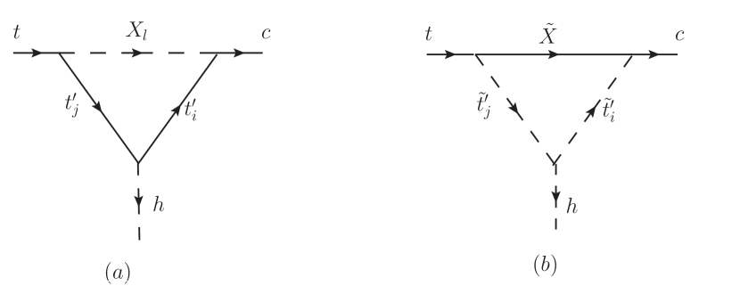
The relevant one-loop vertex diagrams
of BLMSSM are drawn in Fig.1.
Figure 1: The vertex diagrams contributing to the
t → c h → 𝑡 𝑐 ℎ t\rightarrow ch
We could see that the FCNC transitions of new physics are mediated
by the exotic up type quark t ′ superscript 𝑡 ′ t^{\prime} X i subscript 𝑋 𝑖 X_{i} t ~ ′ , X ~ superscript ~ 𝑡 ′ ~ 𝑋
\widetilde{t}^{\prime},\widetilde{X}
In the equations below, m t ′ subscript 𝑚 superscript 𝑡 ′ m_{t^{\prime}} m X subscript 𝑚 𝑋 m_{X} m t ~ ′ subscript 𝑚 superscript ~ 𝑡 ′ m_{\widetilde{t}^{\prime}} m X ~ subscript 𝑚 ~ 𝑋 m_{\widetilde{X}} t ′ superscript 𝑡 ′ t^{\prime} X i subscript 𝑋 𝑖 X_{i} t ~ ′ , X ~ superscript ~ 𝑡 ′ ~ 𝑋
\widetilde{t}^{\prime},\widetilde{X} B i , C i j subscript 𝐵 𝑖 subscript 𝐶 𝑖 𝑗
B_{i},{C}_{ij} ref13
In Fig.1(a), when one-loop diagrams are composed by the neutral
scalar particles X i subscript 𝑋 𝑖 X_{i} 2 / 3 2 3 2/3 t ′ superscript 𝑡 ′ t^{\prime} F L a superscript subscript 𝐹 𝐿 𝑎 F_{L}^{a} F R a superscript subscript 𝐹 𝑅 𝑎 F_{R}^{a}
F L a = i 16 π 2 ∑ i , j , l ( − a 1 m c ( b 1 h 2 m t C 2 + b 2 h 1 m t ′ i ( C 0 + C 1 + 2 C 2 ) + 3 b 2 h 2 m t ′ j C 2 ) ) superscript subscript 𝐹 𝐿 𝑎 𝑖 16 superscript 𝜋 2 subscript 𝑖 𝑗 𝑙
subscript 𝑎 1 subscript 𝑚 𝑐 subscript 𝑏 1 subscript ℎ 2 subscript 𝑚 𝑡 subscript 𝐶 2 subscript 𝑏 2 subscript ℎ 1 subscript 𝑚 subscript superscript 𝑡 ′ 𝑖 subscript 𝐶 0 subscript 𝐶 1 2 subscript 𝐶 2 3 subscript 𝑏 2 subscript ℎ 2 subscript 𝑚 subscript superscript 𝑡 ′ 𝑗 subscript 𝐶 2 \displaystyle F_{L}^{a}=\frac{i}{{16{\pi^{2}}}}\sum_{i,j,\ l}(-{a_{1}}{m_{c}}({b_{1}}{h_{2}}{m_{t}}{C_{2}}+{b_{2}}{h_{1}}{m_{{{t^{\prime}}_{i}}}}({C_{0}}+{C_{1}}+2{C_{2}})+3{b_{2}}{h_{2}}{m_{{{t^{\prime}}_{j}}}}{C_{2}}))
+ a 2 b 2 ( h 1 B 0 + ( h 1 m t ′ i 2 + h 2 m t ′ i m t ′ j ) C 0 ) subscript 𝑎 2 subscript 𝑏 2 subscript ℎ 1 subscript 𝐵 0 subscript ℎ 1 superscript subscript 𝑚 subscript superscript 𝑡 ′ 𝑖 2 subscript ℎ 2 subscript 𝑚 subscript superscript 𝑡 ′ 𝑖 subscript 𝑚 subscript superscript 𝑡 ′ 𝑗 subscript 𝐶 0 \displaystyle\hskip 36.98866pt+{a_{2}}{b_{2}}({h_{1}}{B_{0}}+({h_{1}}m_{{{t^{\prime}}_{i}}}^{2}+{h_{2}}{m_{{{t^{\prime}}_{i}}}}{m_{{{t^{\prime}}_{j}}}}){C_{0}})
+ a 2 b 1 m t ( h 2 m t ′ i ( C 0 + C 1 + C 2 ) + h 1 m t ′ j ( C 1 + C 2 ) ) + a 2 b 2 h 1 m c 2 C 2 subscript 𝑎 2 subscript 𝑏 1 subscript 𝑚 𝑡 subscript ℎ 2 subscript 𝑚 subscript superscript 𝑡 ′ 𝑖 subscript 𝐶 0 subscript 𝐶 1 subscript 𝐶 2 subscript ℎ 1 subscript 𝑚 subscript superscript 𝑡 ′ 𝑗 subscript 𝐶 1 subscript 𝐶 2 subscript 𝑎 2 subscript 𝑏 2 subscript ℎ 1 superscript subscript 𝑚 𝑐 2 subscript 𝐶 2 \displaystyle\hskip 36.98866pt+{a_{2}}{b_{1}}{m_{t}}({h_{2}}{m_{{{t^{\prime}}_{i}}}}({C_{0}}+{C_{1}}+{C_{2}})+{h_{1}}{m_{{{t^{\prime}}_{j}}}}({C_{1}}+{C_{2}}))+{a_{2}}{b_{2}}{h_{1}}{m_{c}}^{2}{C_{2}}
F R a = i 16 π 2 ∑ i , j , l ( − a 2 m c ( b 1 h 2 m t ′ i ( C 0 + C 1 + 2 C 2 ) + b 1 h 1 m t ′ j ( C 1 + 2 C 2 ) + b 2 h 1 m t C 2 ) ) superscript subscript 𝐹 𝑅 𝑎 𝑖 16 superscript 𝜋 2 subscript 𝑖 𝑗 𝑙
subscript 𝑎 2 subscript 𝑚 𝑐 subscript 𝑏 1 subscript ℎ 2 subscript 𝑚 subscript superscript 𝑡 ′ 𝑖 subscript 𝐶 0 subscript 𝐶 1 2 subscript 𝐶 2 subscript 𝑏 1 subscript ℎ 1 subscript 𝑚 subscript superscript 𝑡 ′ 𝑗 subscript 𝐶 1 2 subscript 𝐶 2 subscript 𝑏 2 subscript ℎ 1 subscript 𝑚 𝑡 subscript 𝐶 2 \displaystyle F_{R}^{a}=\frac{i}{{16{\pi^{2}}}}\sum_{i,j,\ l}(-{a_{2}}{m_{c}}({b_{1}}{h_{2}}{m_{{{t^{\prime}}_{i}}}}({C_{0}}+{C_{1}}+2{C_{2}})+{b_{1}}{h_{1}}{m_{{{t^{\prime}}_{j}}}}({C_{1}}+2{C_{2}})+{b_{2}}{h_{1}}{m_{t}}{C_{2}}))
+ a 1 b 1 ( h 2 B 0 + ( h 1 m t ′ i m t ′ j + h 2 m t ′ i 2 ) C 0 ) subscript 𝑎 1 subscript 𝑏 1 subscript ℎ 2 subscript 𝐵 0 subscript ℎ 1 subscript 𝑚 subscript superscript 𝑡 ′ 𝑖 subscript 𝑚 subscript superscript 𝑡 ′ 𝑗 subscript ℎ 2 superscript subscript 𝑚 subscript superscript 𝑡 ′ 𝑖 2 subscript 𝐶 0 \displaystyle\hskip 36.98866pt+{a_{1}}{b_{1}}({h_{2}}{B_{0}}+({h_{1}}{m_{{{t^{\prime}}_{i}}}}{m_{{{t^{\prime}}_{j}}}}+{h_{2}}m_{{{t^{\prime}}_{i}}}^{2}){C_{0}})
+ a 1 b 2 m t ( h 1 m t ′ i ( C 0 + C 1 + C 2 ) + h 2 m t ′ j ( C 1 + C 2 ) ) + a 1 b 1 h 2 m c 2 C 2 subscript 𝑎 1 subscript 𝑏 2 subscript 𝑚 𝑡 subscript ℎ 1 subscript 𝑚 subscript superscript 𝑡 ′ 𝑖 subscript 𝐶 0 subscript 𝐶 1 subscript 𝐶 2 subscript ℎ 2 subscript 𝑚 subscript superscript 𝑡 ′ 𝑗 subscript 𝐶 1 subscript 𝐶 2 subscript 𝑎 1 subscript 𝑏 1 subscript ℎ 2 superscript subscript 𝑚 𝑐 2 subscript 𝐶 2 \displaystyle\hskip 36.98866pt+{a_{1}}{b_{2}}{m_{t}}({h_{1}}{m_{{{t^{\prime}}_{i}}}}({C_{0}}+{C_{1}}+{C_{2}})+{h_{2}}{m_{{{t^{\prime}}_{j}}}}({C_{1}}+{C_{2}}))+{a_{1}}{b_{1}}{h_{2}}{m_{c}}^{2}{C_{2}} (51)
with the Passarino-Veltman integrals
B 0 = B 0 ( p 2 , m t ′ j 2 , m ) X l 2 \displaystyle{B_{0}}={B_{0}}({p^{2}},m_{{{t^{\prime}}_{j}}}^{2},m{{}_{X_{l}}^{2}})
C 0 = C 0 ( p 2 , ( 2 p − p ′ ) 2 , ( p − p ′ ) 2 , m t ′ j 2 , m X l 2 , m t ′ i 2 ) subscript C 0 subscript C 0 superscript 𝑝 2 superscript 2 𝑝 superscript 𝑝 ′ 2 superscript 𝑝 superscript 𝑝 ′ 2 superscript subscript 𝑚 subscript superscript 𝑡 ′ 𝑗 2 superscript subscript 𝑚 subscript 𝑋 𝑙 2 superscript subscript 𝑚 subscript superscript 𝑡 ′ 𝑖 2 \displaystyle{{\rm{C}}_{0}}{\rm{=}}{{\rm{C}}_{0}}\left({{p^{2}},{{(2p-p^{\prime})}^{2}},{{(p-p^{\prime})}^{2}},m_{{{t^{\prime}}_{j}}}^{2},m_{{X_{l}}}^{2},m_{{{t^{\prime}}_{i}}}^{2}}\right)
C 1 , 2 = C 1 , 2 ( ( p − p ′ ) 2 , ( 2 p − p ′ ) 2 , p 2 , m t ′ i 2 , m t ′ j 2 , m X l 2 ) subscript C 1 2
subscript C 1 2
superscript 𝑝 superscript 𝑝 ′ 2 superscript 2 𝑝 superscript 𝑝 ′ 2 superscript 𝑝 2 superscript subscript 𝑚 subscript superscript 𝑡 ′ 𝑖 2 superscript subscript 𝑚 subscript superscript 𝑡 ′ 𝑗 2 superscript subscript 𝑚 subscript 𝑋 𝑙 2 \displaystyle{{\rm{C}}_{1,2}}{\rm{=}}{{\rm{C}}_{1,2}}\left({{{(p-p^{\prime})}^{2}},{{(2p-p^{\prime})}^{2}},{p^{2}},m_{{{t^{\prime}}_{i}}}^{2},m_{{{t^{\prime}}_{j}}}^{2},m_{{X_{l}}}^{2}}\right) (52)
and the relevant coefficients are
a 1 = λ 1 ∗ ( W t ′ † ) 2 i ( Z X † ) l 1 , a 2 = λ 2 ( U t ′ † ) 2 i ( Z X ) 2 l , formulae-sequence subscript 𝑎 1 superscript subscript 𝜆 1 subscript superscript subscript 𝑊 superscript 𝑡 ′ † 2 𝑖 subscript superscript subscript 𝑍 𝑋 † 𝑙 1 subscript 𝑎 2 subscript 𝜆 2 subscript superscript subscript 𝑈 superscript 𝑡 ′ † 2 𝑖 subscript subscript 𝑍 𝑋 2 𝑙 \displaystyle{a_{1}}=\lambda_{1}^{*}{(W_{t^{\prime}}^{\dagger})_{2i}}{(Z_{X}^{\dagger})_{l1}},{\kern 1.0pt}{\kern 1.0pt}{\kern 1.0pt}{\kern 1.0pt}{\kern 1.0pt}{\kern 1.0pt}{\kern 1.0pt}{\kern 1.0pt}{\kern 1.0pt}{\kern 1.0pt}{\kern 1.0pt}{\kern 1.0pt}{\kern 1.0pt}{\kern 1.0pt}{\kern 1.0pt}{\kern 1.0pt}{\kern 1.0pt}{\kern 1.0pt}{\kern 1.0pt}{\kern 1.0pt}{\kern 1.0pt}{\kern 1.0pt}{\kern 1.0pt}{\kern 1.0pt}{\kern 1.0pt}{\kern 1.0pt}{\kern 1.0pt}{a_{2}}={\lambda_{2}}{(U_{t^{\prime}}^{\dagger})_{2i}}{({Z_{X}})_{2l}},
b 1 = λ 2 ∗ ( U t ′ ) j 2 ( Z X † ) l 2 , b 2 = λ 1 ( W t ′ ) j 2 ( Z X ) 1 l , formulae-sequence subscript 𝑏 1 superscript subscript 𝜆 2 subscript subscript 𝑈 superscript 𝑡 ′ 𝑗 2 subscript superscript subscript 𝑍 𝑋 † 𝑙 2 subscript 𝑏 2 subscript 𝜆 1 subscript subscript 𝑊 superscript 𝑡 ′ 𝑗 2 subscript subscript 𝑍 𝑋 1 𝑙 \displaystyle{b_{1}}=\lambda_{2}^{*}{({U_{t^{\prime}}})_{j2}}{(Z_{X}^{\dagger})_{l2}},{\kern 1.0pt}{\kern 1.0pt}{\kern 1.0pt}{\kern 1.0pt}{\kern 1.0pt}{\kern 1.0pt}{\kern 1.0pt}{\kern 1.0pt}{\kern 1.0pt}{\kern 1.0pt}{\kern 1.0pt}{\kern 1.0pt}{\kern 1.0pt}{\kern 1.0pt}{\kern 1.0pt}{\kern 1.0pt}{\kern 1.0pt}{\kern 1.0pt}{\kern 1.0pt}{\kern 1.0pt}{\kern 1.0pt}{\kern 1.0pt}{\kern 1.0pt}{\kern 1.0pt}{\kern 1.0pt}{\kern 1.0pt}{\kern 1.0pt}{\kern 1.0pt}{b_{2}}={\lambda_{1}}{({W_{t^{\prime}}})_{j2}}{({Z_{X}})_{1l}},
h 1 = Y u 4 ( U t ′ † ) i 1 ( W t ′ ) 2 j cos α + Y u 5 ( U t ′ † ) i 2 ( W t ′ ) 1 j sin α , subscript ℎ 1 subscript 𝑌 subscript 𝑢 4 subscript superscript subscript 𝑈 superscript 𝑡 ′ † 𝑖 1 subscript subscript 𝑊 superscript 𝑡 ′ 2 𝑗 𝛼 subscript 𝑌 subscript 𝑢 5 subscript superscript subscript 𝑈 superscript 𝑡 ′ † 𝑖 2 subscript subscript 𝑊 superscript 𝑡 ′ 1 𝑗 𝛼 \displaystyle{h_{1}}={Y_{{u_{4}}}}{(U_{t^{\prime}}^{\dagger})_{i1}}{({W_{t^{\prime}}})_{2j}}\cos\alpha+{Y_{{u_{5}}}}{(U_{t^{\prime}}^{\dagger})_{i2}}{({W_{t^{\prime}}})_{1j}}\sin\alpha,
h 2 = Y u 4 ( W t ′ † ) i 2 ( U t ′ ) 1 j cos α + Y u 5 ( W t ′ † ) i 1 ( U t ′ ) 2 j sin α , subscript ℎ 2 subscript 𝑌 subscript 𝑢 4 subscript superscript subscript 𝑊 superscript 𝑡 ′ † 𝑖 2 subscript subscript 𝑈 superscript 𝑡 ′ 1 𝑗 𝛼 subscript 𝑌 subscript 𝑢 5 subscript superscript subscript 𝑊 superscript 𝑡 ′ † 𝑖 1 subscript subscript 𝑈 superscript 𝑡 ′ 2 𝑗 𝛼 \displaystyle{h_{2}}={Y_{{u_{4}}}}{(W_{t^{\prime}}^{\dagger})_{i2}}{({U_{t^{\prime}}})_{1j}}\cos\alpha+{Y_{{u_{5}}}}{(W_{t^{\prime}}^{\dagger})_{i1}}{({U_{t^{\prime}}})_{2j}}\sin\alpha, (53)
In Fig.1(b), when one-loop diagrams are composed by the
superpartners t ~ ′ superscript ~ 𝑡 ′ \widetilde{t}^{\prime} X ~ ~ 𝑋 \widetilde{X} F L b superscript subscript 𝐹 𝐿 𝑏 F_{L}^{b} F R b superscript subscript 𝐹 𝑅 𝑏 F_{R}^{b}
F L b = i 16 π 2 ∑ i , j ( a 4 b 4 m X ~ C 0 − a 3 b 4 m c C 1 − a 4 b 3 m t C 2 ) ( cos α ξ u − sin α ξ d ) superscript subscript 𝐹 𝐿 𝑏 𝑖 16 superscript 𝜋 2 subscript 𝑖 𝑗
subscript 𝑎 4 subscript 𝑏 4 subscript 𝑚 ~ 𝑋 subscript 𝐶 0 subscript 𝑎 3 subscript 𝑏 4 subscript 𝑚 𝑐 subscript 𝐶 1 subscript 𝑎 4 subscript 𝑏 3 subscript 𝑚 𝑡 subscript 𝐶 2 𝛼 subscript 𝜉 𝑢 𝛼 subscript 𝜉 𝑑 \displaystyle F_{L}^{b}=\frac{i}{{16{\pi^{2}}}}\sum_{i,j}({a_{4}}{b_{4}}{m_{\tilde{X}}}{C_{0}}-{a_{3}}{b_{4}}{m_{c}}{C_{1}}-{a_{4}}{b_{3}}{m_{t}}{C_{2}})(\cos{\alpha}{\xi_{u}}-\sin{\alpha}{\xi_{d}})
F R b = i 16 π 2 ∑ i , j ( a 4 b 4 m X ~ C 0 − a 3 b 4 m c C 1 − a 4 b 3 m t C 2 ) ( cos α ξ u − sin α ξ d ) superscript subscript 𝐹 𝑅 𝑏 𝑖 16 superscript 𝜋 2 subscript 𝑖 𝑗
subscript 𝑎 4 subscript 𝑏 4 subscript 𝑚 ~ 𝑋 subscript 𝐶 0 subscript 𝑎 3 subscript 𝑏 4 subscript 𝑚 𝑐 subscript 𝐶 1 subscript 𝑎 4 subscript 𝑏 3 subscript 𝑚 𝑡 subscript 𝐶 2 𝛼 subscript 𝜉 𝑢 𝛼 subscript 𝜉 𝑑 \displaystyle F_{R}^{b}=\frac{i}{{16{\pi^{2}}}}\sum_{i,j}({a_{4}}{b_{4}}{m_{\tilde{X}}}{C_{0}}-{a_{3}}{b_{4}}{m_{c}}{C_{1}}-{a_{4}}{b_{3}}{m_{t}}{C_{2}})(\cos{\alpha}{\xi_{u}}-\sin{\alpha}{\xi_{d}}) (54)
with
C 0 = C 0 ( p 2 , p ′ 2 , ( p − p ′ ) 2 , m t ~ ′ i 2 , m X ~ 2 , m t ~ ′ j 2 ) subscript C 0 subscript C 0 superscript 𝑝 2 superscript superscript 𝑝 ′ 2 superscript 𝑝 superscript 𝑝 ′ 2 superscript subscript 𝑚 subscript superscript ~ 𝑡 ′ 𝑖 2 superscript subscript 𝑚 ~ 𝑋 2 superscript subscript 𝑚 subscript superscript ~ 𝑡 ′ 𝑗 2 \displaystyle{{\rm{C}}_{0}}{\rm{=}}{{\rm{C}}_{0}}\left({{p^{2}},{{p^{\prime}}^{2}},{{(p-p^{\prime})}^{2}},m_{{{\tilde{t}^{\prime}}_{i}}}^{2},m_{\tilde{X}}^{2},m_{{{\tilde{t}^{\prime}}_{j}}}^{2}}\right)
C 1 , 2 = C 1 , 2 ( p 2 , ( p − p ′ ) 2 , p ′ 2 , m X ~ 2 , m t ~ ′ i 2 , m t ~ ′ j 2 ) subscript C 1 2
subscript C 1 2
superscript 𝑝 2 superscript 𝑝 superscript 𝑝 ′ 2 superscript superscript 𝑝 ′ 2 superscript subscript 𝑚 ~ 𝑋 2 superscript subscript 𝑚 subscript superscript ~ 𝑡 ′ 𝑖 2 superscript subscript 𝑚 subscript superscript ~ 𝑡 ′ 𝑗 2 \displaystyle{{\rm{C}}_{1,2}}{\rm{=}}{{\rm{C}}_{1,2}}\left({{p^{2}},{{(p-p^{\prime})}^{2}},{{p^{\prime}}^{2}},m_{\tilde{X}}^{2},m_{{{\tilde{t}^{\prime}}_{i}}}^{2},m_{{{\tilde{t}^{\prime}}_{j}}}^{2}}\right) (55)
and the relevant coefficients are
a 3 = λ 2 ∗ ( Z t ~ ′ † ) i 4 , a 4 = λ 1 ( Z t ~ ′ † ) i 3 , formulae-sequence subscript 𝑎 3 superscript subscript 𝜆 2 subscript superscript subscript 𝑍 superscript ~ 𝑡 ′ † 𝑖 4 subscript 𝑎 4 subscript 𝜆 1 subscript superscript subscript 𝑍 superscript ~ 𝑡 ′ † 𝑖 3 \displaystyle{a_{3}}=\lambda_{2}^{*}{(Z_{\tilde{t}^{\prime}}^{\dagger})_{i4}},{\kern 1.0pt}{\kern 1.0pt}{\kern 1.0pt}{\kern 1.0pt}{\kern 1.0pt}{\kern 1.0pt}{\kern 1.0pt}{\kern 1.0pt}{\kern 1.0pt}{\kern 1.0pt}{\kern 1.0pt}{\kern 1.0pt}{\kern 1.0pt}{\kern 1.0pt}{\kern 1.0pt}{\kern 1.0pt}{\kern 1.0pt}{\kern 1.0pt}{\kern 1.0pt}{\kern 1.0pt}{\kern 1.0pt}{\kern 1.0pt}{\kern 1.0pt}{\kern 1.0pt}{\kern 1.0pt}{\kern 1.0pt}{\kern 1.0pt}{\kern 1.0pt}{\kern 1.0pt}{\kern 1.0pt}{\kern 1.0pt}{\kern 1.0pt}{\kern 1.0pt}{\kern 1.0pt}{\kern 1.0pt}{\kern 1.0pt}{\kern 1.0pt}{a_{4}}={\lambda_{1}}{(Z_{\tilde{t}^{\prime}}^{\dagger})_{i3}},
b 3 = λ 1 ∗ ( Z t ~ ′ ) 3 j , b 4 = λ 2 ( Z t ~ ′ ) 4 j , formulae-sequence subscript 𝑏 3 superscript subscript 𝜆 1 subscript subscript 𝑍 superscript ~ 𝑡 ′ 3 𝑗 subscript 𝑏 4 subscript 𝜆 2 subscript subscript 𝑍 superscript ~ 𝑡 ′ 4 𝑗 \displaystyle{b_{3}}=\lambda_{1}^{*}{({Z_{\tilde{t}^{\prime}}})_{3j}},{\kern 1.0pt}{\kern 1.0pt}{\kern 1.0pt}{\kern 1.0pt}{\kern 1.0pt}{\kern 1.0pt}{\kern 1.0pt}{\kern 1.0pt}{\kern 1.0pt}{\kern 1.0pt}{\kern 1.0pt}{\kern 1.0pt}{\kern 1.0pt}{\kern 1.0pt}{\kern 1.0pt}{\kern 1.0pt}{\kern 1.0pt}{\kern 1.0pt}{\kern 1.0pt}{\kern 1.0pt}{\kern 1.0pt}{\kern 1.0pt}{\kern 1.0pt}{\kern 1.0pt}{\kern 1.0pt}{\kern 1.0pt}{\kern 1.0pt}{\kern 1.0pt}{\kern 1.0pt}{\kern 1.0pt}{\kern 1.0pt}{\kern 1.0pt}{\kern 1.0pt}{\kern 1.0pt}{\kern 1.0pt}{\kern 1.0pt}{\kern 1.0pt}{b_{4}}={\lambda_{2}}{({Z_{\tilde{t}^{\prime}}})_{4j}}, (56)
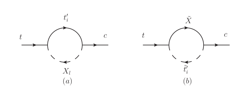
In Fig.2 we present the relevant self-energy diagrams of the rare
decay t → c h → 𝑡 𝑐 ℎ t\rightarrow ch
Figure 2: The self-energy diagrams contributing to the
t → c h → 𝑡 𝑐 ℎ t\rightarrow ch
As in Ref.ref6
Σ t c ( k ) ≡ k̸ Σ L ( k 2 ) P L + k̸ Σ R ( k 2 ) P R + m t ( Σ L s ( k 2 ) P L + Σ R s ( k 2 ) P R ) . subscript Σ 𝑡 𝑐 𝑘 italic-k̸ subscript Σ 𝐿 superscript 𝑘 2 subscript 𝑃 𝐿 italic-k̸ subscript Σ 𝑅 superscript 𝑘 2 subscript 𝑃 𝑅 subscript 𝑚 𝑡 subscript Σ 𝐿 𝑠 superscript 𝑘 2 subscript 𝑃 𝐿 subscript Σ 𝑅 𝑠 superscript 𝑘 2 subscript 𝑃 𝑅 \displaystyle{\Sigma_{tc}}(k)\equiv\not{k}{\Sigma_{L}}({k^{2}}){P_{L}}+\not k{\Sigma_{R}}({k^{2}}){P_{R}}+{m_{t}}({\Sigma_{Ls}}({k^{2}}){P_{L}}+{\Sigma_{Rs}}({k^{2}}){P_{R}}). (57)
Here m t subscript 𝑚 𝑡 m_{t} Σ Σ \Sigma ref6 Σ Σ \Sigma
− i T S c = − i g m t 2 m W sin β 1 m c 2 − m t 2 c ¯ ( p ) { \displaystyle-i{T_{Sc}}=\frac{{-ig{m_{t}}}}{{2{m_{W}}\sin\beta}}\frac{1}{{m_{c}^{2}-m_{t}^{2}}}\bar{c}(p)\left\{{}\right.
( P L cos α [ m c 2 Σ R ( m c 2 ) + m c m t ( Σ R s ( m c 2 ) + Σ L ( m c 2 ) ) + m t 2 Σ L s ( m c 2 ) ] \displaystyle{\kern 1.0pt}{\kern 1.0pt}{\kern 1.0pt}{\kern 1.0pt}{\kern 1.0pt}{\kern 1.0pt}{\kern 1.0pt}{\kern 1.0pt}{\kern 1.0pt}{\kern 1.0pt}{\kern 1.0pt}{\kern 1.0pt}{\kern 1.0pt}{\kern 1.0pt}{\kern 1.0pt}{\kern 1.0pt}{\kern 1.0pt}{\kern 1.0pt}{\kern 1.0pt}{\kern 1.0pt}{\kern 1.0pt}{\kern 1.0pt}{\kern 1.0pt}{\kern 1.0pt}{\kern 1.0pt}{\kern 1.0pt}{\kern 1.0pt}{\kern 1.0pt}{\kern 1.0pt}{\kern 1.0pt}{\kern 1.0pt}{\kern 1.0pt}{\kern 1.0pt}{\kern 1.0pt}{\kern 1.0pt}({P_{L}}\cos\alpha[m_{c}^{2}{\Sigma_{R}}(m_{c}^{2})+{m_{c}}{m_{t}}({\Sigma_{Rs}}(m_{c}^{2})+{\Sigma_{L}}(m_{c}^{2}))+m_{t}^{2}{\Sigma_{Ls}}(m_{c}^{2})]
+ P R cos α [ L ↔ R ] } t ( p ′ ) \displaystyle\left.{{\kern 1.0pt}{\kern 1.0pt}{\kern 1.0pt}{\kern 1.0pt}{\kern 1.0pt}{\kern 1.0pt}{\kern 1.0pt}{\kern 1.0pt}{\kern 1.0pt}{\kern 1.0pt}{\kern 1.0pt}{\kern 1.0pt}{\kern 1.0pt}{\kern 1.0pt}{\kern 1.0pt}{\kern 1.0pt}{\kern 1.0pt}{\kern 1.0pt}{\kern 1.0pt}{\kern 1.0pt}{\kern 1.0pt}{\kern 1.0pt}{\kern 1.0pt}{\kern 1.0pt}{\kern 1.0pt}{\kern 1.0pt}{\kern 1.0pt}{\kern 1.0pt}{\kern 1.0pt}{\kern 1.0pt}{\kern 1.0pt}{\kern 1.0pt}{\kern 1.0pt}+{P_{R}}\cos\alpha[L\leftrightarrow R]}\right\}t(p^{\prime})
− i T S t = − i g m c 2 m W sin β m t m c 2 − m t 2 c ¯ ( p ) { \displaystyle-i{T_{St}}=\frac{{-ig{m_{c}}}}{{2{m_{W}}\sin\beta}}\frac{{{m_{t}}}}{{m_{c}^{2}-m_{t}^{2}}}\bar{c}(p)\left\{{}\right.
( P L cos α [ m t ( Σ L ( m t 2 ) + Σ R s ( m t 2 ) ) + m c ( Σ R ( m t 2 ) + Σ L s ( m t 2 ) ) ] \displaystyle{\kern 1.0pt}{\kern 1.0pt}{\kern 1.0pt}{\kern 1.0pt}{\kern 1.0pt}{\kern 1.0pt}{\kern 1.0pt}{\kern 1.0pt}{\kern 1.0pt}{\kern 1.0pt}{\kern 1.0pt}{\kern 1.0pt}{\kern 1.0pt}{\kern 1.0pt}{\kern 1.0pt}{\kern 1.0pt}{\kern 1.0pt}{\kern 1.0pt}{\kern 1.0pt}{\kern 1.0pt}{\kern 1.0pt}{\kern 1.0pt}{\kern 1.0pt}{\kern 1.0pt}{\kern 1.0pt}{\kern 1.0pt}{\kern 1.0pt}{\kern 1.0pt}{\kern 1.0pt}{\kern 1.0pt}{\kern 1.0pt}{\kern 1.0pt}{\kern 1.0pt}{\kern 1.0pt}({P_{L}}\cos\alpha[{m_{t}}({\Sigma_{L}}(m_{t}^{2})+{\Sigma_{Rs}}(m_{t}^{2}))+{m_{c}}({\Sigma_{R}}(m_{t}^{2})+{\Sigma_{Ls}}(m_{t}^{2}))]
+ P R cos α [ L ↔ R ] } t ( p ′ ) \displaystyle{\kern 1.0pt}{\kern 1.0pt}{\kern 1.0pt}{\kern 1.0pt}{\kern 1.0pt}{\kern 1.0pt}{\kern 1.0pt}{\kern 1.0pt}{\kern 1.0pt}{\kern 1.0pt}{\kern 1.0pt}{\kern 1.0pt}{\kern 1.0pt}{\kern 1.0pt}{\kern 1.0pt}{\kern 1.0pt}{\kern 1.0pt}{\kern 1.0pt}{\kern 1.0pt}{\kern 1.0pt}{\kern 1.0pt}{\kern 1.0pt}{\kern 1.0pt}{\kern 1.0pt}{\kern 1.0pt}{\kern 1.0pt}{\kern 1.0pt}{\kern 1.0pt}{\kern 1.0pt}{\kern 1.0pt}{\kern 1.0pt}{\kern 1.0pt}{\kern 1.0pt}{\kern 1.0pt}\left.{+{P_{R}}\cos\alpha[L\leftrightarrow R]}\right\}t(p^{\prime}) (58)
Comparing with Eq. 16, the corresponding contribution to the form
factors F L subscript 𝐹 𝐿 F_{L} F R subscript 𝐹 𝑅 F_{R}
Using the couplings above, we could get the Σ Σ \Sigma
Σ L ( k 2 ) = i 16 π 2 ∑ i , l a 1 b 2 ( B 0 ( k 2 , m X l 2 , m t ′ 2 ) + B 1 ( k 2 , m X l 2 , m t ′ 2 ) ) subscript Σ 𝐿 superscript 𝑘 2 𝑖 16 superscript 𝜋 2 subscript 𝑖 𝑙
subscript 𝑎 1 subscript 𝑏 2 subscript 𝐵 0 superscript 𝑘 2 superscript subscript 𝑚 subscript 𝑋 𝑙 2 superscript subscript 𝑚 superscript 𝑡 ′ 2 subscript 𝐵 1 superscript 𝑘 2 superscript subscript 𝑚 subscript 𝑋 𝑙 2 superscript subscript 𝑚 superscript 𝑡 ′ 2 \displaystyle{\Sigma_{L}}({k^{2}})=\frac{i}{{16{\pi^{2}}}}\sum_{i,\ l}{a_{1}}{b_{2}}({B_{0}}({k^{2}},m_{{X_{l}}}^{2},m_{t^{\prime}}^{2})+{B_{1}}({k^{2}},m_{{X_{l}}}^{2},m_{t^{\prime}}^{2}))
Σ R ( k 2 ) = i 16 π 2 ∑ i , l a 2 b 1 ( B 0 ( k 2 , m X l 2 , m t ′ 2 ) + B 1 ( k 2 , m X l 2 , m t ′ 2 ) ) subscript Σ 𝑅 superscript 𝑘 2 𝑖 16 superscript 𝜋 2 subscript 𝑖 𝑙
subscript 𝑎 2 subscript 𝑏 1 subscript 𝐵 0 superscript 𝑘 2 superscript subscript 𝑚 subscript 𝑋 𝑙 2 superscript subscript 𝑚 superscript 𝑡 ′ 2 subscript 𝐵 1 superscript 𝑘 2 superscript subscript 𝑚 subscript 𝑋 𝑙 2 superscript subscript 𝑚 superscript 𝑡 ′ 2 \displaystyle{\Sigma_{R}}({k^{2}})=\frac{i}{{16{\pi^{2}}}}\sum_{i,\ l}{a_{2}}{b_{1}}({B_{0}}({k^{2}},m_{{X_{l}}}^{2},m_{t^{\prime}}^{2})+{B_{1}}({k^{2}},m_{{X_{l}}}^{2},m_{t^{\prime}}^{2}))
m t Σ L s ( k 2 ) = i 16 π 2 ∑ i , l a 2 b 2 m t ′ B 0 ( k 2 , m X l 2 , m t ′ 2 ) subscript 𝑚 𝑡 subscript Σ 𝐿 𝑠 superscript 𝑘 2 𝑖 16 superscript 𝜋 2 subscript 𝑖 𝑙
subscript 𝑎 2 subscript 𝑏 2 subscript 𝑚 superscript 𝑡 ′ subscript 𝐵 0 superscript 𝑘 2 superscript subscript 𝑚 subscript 𝑋 𝑙 2 superscript subscript 𝑚 superscript 𝑡 ′ 2 \displaystyle{m_{t}}{\Sigma_{Ls}}({k^{2}})=\frac{i}{{16{\pi^{2}}}}\sum_{i,\ l}{a_{2}}{b_{2}}{m_{t^{\prime}}}{B_{0}}({k^{2}},m_{{X_{l}}}^{2},m_{t^{\prime}}^{2})
m t Σ R s ( k 2 ) = i 16 π 2 ∑ i , l a 1 b 1 m t ′ B 0 ( k 2 , m X l 2 , m t ′ 2 ) subscript 𝑚 𝑡 subscript Σ 𝑅 𝑠 superscript 𝑘 2 𝑖 16 superscript 𝜋 2 subscript 𝑖 𝑙
subscript 𝑎 1 subscript 𝑏 1 subscript 𝑚 superscript 𝑡 ′ subscript 𝐵 0 superscript 𝑘 2 superscript subscript 𝑚 subscript 𝑋 𝑙 2 superscript subscript 𝑚 superscript 𝑡 ′ 2 \displaystyle{m_{t}}{\Sigma_{Rs}}({k^{2}})=\frac{i}{{16{\pi^{2}}}}\sum_{i,\ l}{a_{1}}{b_{1}}{m_{t^{\prime}}}{B_{0}}({k^{2}},m_{{X_{l}}}^{2},m_{t^{\prime}}^{2}) (59)
with B 0 , 1 subscript 𝐵 0 1
B_{0,1} Σ Σ \Sigma
Σ L ( k 2 ) = i 16 π 2 ∑ i a 3 b 4 ( B 0 ( k 2 , m t ~ ′ 2 , m X ~ 2 ) + B 1 ( k 2 , m t ~ ′ 2 , m X ~ 2 ) ) subscript Σ 𝐿 superscript 𝑘 2 𝑖 16 superscript 𝜋 2 subscript 𝑖 subscript 𝑎 3 subscript 𝑏 4 subscript 𝐵 0 superscript 𝑘 2 superscript subscript 𝑚 superscript ~ 𝑡 ′ 2 superscript subscript 𝑚 ~ 𝑋 2 subscript 𝐵 1 superscript 𝑘 2 superscript subscript 𝑚 superscript ~ 𝑡 ′ 2 superscript subscript 𝑚 ~ 𝑋 2 \displaystyle{\Sigma_{L}}({k^{2}})=\frac{i}{{16{\pi^{2}}}}\sum_{i}{a_{3}}{b_{4}}({B_{0}}({k^{2}},m_{\tilde{t}^{\prime}}^{2},m_{\tilde{X}}^{2})+{B_{1}}({k^{2}},m_{\tilde{t}^{\prime}}^{2},m_{\tilde{X}}^{2}))
Σ R ( k 2 ) = i 16 π 2 ∑ i a 4 b 3 ( B 0 ( k 2 , m t ~ ′ 2 , m X ~ 2 ) + B 1 ( k 2 , m t ~ ′ 2 , m X ~ 2 ) ) subscript Σ 𝑅 superscript 𝑘 2 𝑖 16 superscript 𝜋 2 subscript 𝑖 subscript 𝑎 4 subscript 𝑏 3 subscript 𝐵 0 superscript 𝑘 2 superscript subscript 𝑚 superscript ~ 𝑡 ′ 2 superscript subscript 𝑚 ~ 𝑋 2 subscript 𝐵 1 superscript 𝑘 2 superscript subscript 𝑚 superscript ~ 𝑡 ′ 2 superscript subscript 𝑚 ~ 𝑋 2 \displaystyle{\Sigma_{R}}({k^{2}})=\frac{i}{{16{\pi^{2}}}}\sum_{i}{a_{4}}{b_{3}}({B_{0}}({k^{2}},m_{\tilde{t}^{\prime}}^{2},m_{\tilde{X}}^{2})+{B_{1}}({k^{2}},m_{\tilde{t}^{\prime}}^{2},m_{\tilde{X}}^{2}))
m t Σ L s ( k 2 ) = i 16 π 2 ∑ i a 4 b 4 m t ~ ′ B 0 ( k 2 , m t ~ ′ 2 , m X ~ 2 ) subscript 𝑚 𝑡 subscript Σ 𝐿 𝑠 superscript 𝑘 2 𝑖 16 superscript 𝜋 2 subscript 𝑖 subscript 𝑎 4 subscript 𝑏 4 subscript 𝑚 superscript ~ 𝑡 ′ subscript 𝐵 0 superscript 𝑘 2 superscript subscript 𝑚 superscript ~ 𝑡 ′ 2 superscript subscript 𝑚 ~ 𝑋 2 \displaystyle{m_{t}}{\Sigma_{Ls}}({k^{2}})=\frac{i}{{16{\pi^{2}}}}\sum_{i}{a_{4}}{b_{4}}{m_{\tilde{t}^{\prime}}}{B_{0}}({k^{2}},m_{\tilde{t}^{\prime}}^{2},m_{\tilde{X}}^{2})
m t Σ R s ( k 2 ) = i 16 π 2 ∑ i a 3 b 3 m t ~ ′ B 0 ( k 2 , m t ~ ′ 2 , m X ~ 2 ) subscript 𝑚 𝑡 subscript Σ 𝑅 𝑠 superscript 𝑘 2 𝑖 16 superscript 𝜋 2 subscript 𝑖 subscript 𝑎 3 subscript 𝑏 3 subscript 𝑚 superscript ~ 𝑡 ′ subscript 𝐵 0 superscript 𝑘 2 superscript subscript 𝑚 superscript ~ 𝑡 ′ 2 superscript subscript 𝑚 ~ 𝑋 2 \displaystyle{m_{t}}{\Sigma_{Rs}}({k^{2}})=\frac{i}{{16{\pi^{2}}}}\sum_{i}{a_{3}}{b_{3}}{m_{\tilde{t}^{\prime}}}{B_{0}}({k^{2}},m_{\tilde{t}^{\prime}}^{2},m_{\tilde{X}}^{2}) (60)
IV Numerical analysis
In general case, the partial widths of t → c h → 𝑡 𝑐 ℎ t\rightarrow ch ref6
Γ ( t → c h ) = g 2 32 π m t 3 λ 1 / 2 ( m t 2 , m h 2 , m c 2 ) Γ → 𝑡 𝑐 ℎ superscript 𝑔 2 32 𝜋 superscript subscript 𝑚 𝑡 3 superscript 𝜆 1 2 superscript subscript 𝑚 𝑡 2 superscript subscript 𝑚 ℎ 2 superscript subscript 𝑚 𝑐 2 \displaystyle\Gamma(t\to ch)=\frac{{{g^{2}}}}{{32\pi m_{t}^{3}}}{\lambda^{1/2}}(m_{t}^{2},m_{h}^{2},m_{c}^{2})
× [ ( m t 2 + m c 2 − m h 2 ) ( | F L | 2 + | F R | 2 ) + 2 m t m c ( F L F R ∗ + F L ∗ F R ) ] absent delimited-[] superscript subscript 𝑚 𝑡 2 superscript subscript 𝑚 𝑐 2 superscript subscript 𝑚 ℎ 2 superscript subscript 𝐹 𝐿 2 superscript subscript 𝐹 𝑅 2 2 subscript 𝑚 𝑡 subscript 𝑚 𝑐 subscript 𝐹 𝐿 superscript subscript 𝐹 𝑅 superscript subscript 𝐹 𝐿 subscript 𝐹 𝑅 \displaystyle{\kern 1.0pt}{\kern 1.0pt}{\kern 1.0pt}{\kern 1.0pt}{\kern 1.0pt}{\kern 1.0pt}{\kern 1.0pt}{\kern 1.0pt}{\kern 1.0pt}{\kern 1.0pt}{\kern 1.0pt}{\kern 1.0pt}{\kern 1.0pt}{\kern 1.0pt}{\kern 1.0pt}{\kern 1.0pt}{\kern 1.0pt}{\kern 1.0pt}{\kern 1.0pt}{\kern 1.0pt}{\kern 1.0pt}{\kern 1.0pt}{\kern 1.0pt}{\kern 1.0pt}{\kern 1.0pt}{\kern 1.0pt}{\kern 1.0pt}{\kern 1.0pt}{\kern 1.0pt}{\kern 1.0pt}{\kern 1.0pt}{\kern 1.0pt}{\kern 1.0pt}{\kern 1.0pt}{\kern 1.0pt}{\kern 1.0pt}{\kern 1.0pt}{\kern 1.0pt}{\kern 1.0pt}{\kern 1.0pt}{\kern 1.0pt}{\kern 1.0pt}{\kern 1.0pt}{\kern 1.0pt}{\kern 1.0pt}{\kern 1.0pt}{\kern 1.0pt}{\kern 1.0pt}{\kern 1.0pt}{\kern 1.0pt}{\kern 1.0pt}{\kern 1.0pt}{\kern 1.0pt}{\kern 1.0pt}{\kern 1.0pt}{\kern 1.0pt}{\kern 1.0pt}{\kern 1.0pt}{\kern 1.0pt}{\kern 1.0pt}\times\left[{\left({m_{t}^{2}+m_{c}^{2}-m_{h}^{2}}\right)\left({{{\left|{{F_{L}}}\right|}^{2}}+{{\left|{{F_{R}}}\right|}^{2}}}\right)+2{m_{t}}{m_{c}}\left({{F_{L}}F_{R}^{*}+F_{L}^{*}{F_{R}}}\right)}\right] (61)
with λ ( x 2 , y 2 , z 2 ) = ( x 2 − ( y + z ) 2 ) ( x 2 − ( y − z ) 2 ) 𝜆 superscript 𝑥 2 superscript 𝑦 2 superscript 𝑧 2 superscript 𝑥 2 superscript 𝑦 𝑧 2 superscript 𝑥 2 superscript 𝑦 𝑧 2 \lambda({x^{2}},{y^{2}},{z^{2}})=({x^{2}}-{(y+z)^{2}})({x^{2}}-{(y-z)^{2}})
F L = F L B L S S M + F L M S S M + F L S M subscript 𝐹 𝐿 superscript subscript 𝐹 𝐿 𝐵 𝐿 𝑆 𝑆 𝑀 superscript subscript 𝐹 𝐿 𝑀 𝑆 𝑆 𝑀 superscript subscript 𝐹 𝐿 𝑆 𝑀 \displaystyle{F_{L}}=F_{L}^{BLSSM}+F_{L}^{MSSM}+F_{L}^{SM}
F R = F R B L S S M + F R M S S M + F R S M subscript 𝐹 𝑅 superscript subscript 𝐹 𝑅 𝐵 𝐿 𝑆 𝑆 𝑀 superscript subscript 𝐹 𝑅 𝑀 𝑆 𝑆 𝑀 superscript subscript 𝐹 𝑅 𝑆 𝑀 \displaystyle{F_{R}}=F_{R}^{BLSSM}+F_{R}^{MSSM}+F_{R}^{SM} (62)
In our calculation,we will use the form factors of MSSM F L , R M S S M superscript subscript 𝐹 𝐿 𝑅
𝑀 𝑆 𝑆 𝑀 F_{L,R}^{MSSM} ref6 10 − 13 superscript 10 13 10^{-13} ref5
To compute the branching ratio, we take the SM charged-current
two-body decay t → b W → 𝑡 𝑏 𝑊 t\rightarrow bW t 𝑡 t Γ ( t → b W + ) = 1.466 | V t b | 2 Γ → 𝑡 𝑏 superscript 𝑊 1.466 superscript subscript 𝑉 𝑡 𝑏 2 \Gamma(t\rightarrow bW^{+})=1.466|V_{tb}|^{2}
B r ( t → c h ) = Γ ( t → c h ) Γ ( t → b W + ) 𝐵 𝑟 → 𝑡 𝑐 ℎ Γ → 𝑡 𝑐 ℎ Γ → 𝑡 𝑏 superscript 𝑊 \displaystyle Br(t\to ch)=\frac{{\Gamma(t\to ch)}}{{\Gamma(t\to b{W^{+}})}} (63)
To reduce the number of free parameters in our numerical analysis,
the parameters are adopted as Ref.ref11 ; ref12 2 × 2 2 2 2\times 2 125.9 125.9 125.9 h → γ γ → ℎ 𝛾 𝛾 h\rightarrow\gamma\gamma h → V V ∗ ( V = Z , W ) → ℎ 𝑉 superscript 𝑉 𝑉 𝑍 𝑊
h\rightarrow VV^{*}\;(V=Z,\;W) ref11
B 4 = 3 2 , v B t = v B 2 + v ¯ B 2 = 3 T e V , formulae-sequence subscript 𝐵 4 3 2 subscript 𝑣 subscript 𝐵 𝑡 superscript subscript 𝑣 𝐵 2 superscript subscript ¯ 𝑣 𝐵 2 3 T e V \displaystyle{B_{4}}=\frac{3}{2},{\kern 1.0pt}{\kern 1.0pt}{\kern 1.0pt}{\kern 1.0pt}{\kern 1.0pt}{\kern 1.0pt}{\kern 1.0pt}{\kern 1.0pt}{\kern 1.0pt}{\kern 1.0pt}{v_{{B_{t}}}}=\sqrt{v_{B}^{2}+\bar{v}_{B}^{2}}=3{\rm{TeV}},
tan β = tan β B = 2 , 𝛽 subscript 𝛽 𝐵 2 \displaystyle\tan\beta=\tan{\beta_{B}}=2,
m U ~ 4 = m Q ~ 5 = m U ~ 5 = 1 T e V , subscript 𝑚 subscript ~ 𝑈 4 subscript 𝑚 subscript ~ 𝑄 5 subscript 𝑚 subscript ~ 𝑈 5 1 T e V \displaystyle{m_{{{\tilde{U}}_{4}}}}={m_{{{\tilde{Q}}_{5}}}}={m_{{{\tilde{U}}_{5}}}}=1{\rm{TeV}},
A u 4 = A u 5 = 500 G e V , subscript 𝐴 subscript 𝑢 4 subscript 𝐴 subscript 𝑢 5 500 G e V \displaystyle{A_{{u_{4}}}}={A_{{u_{5}}}}=500{\rm{GeV}},
A B U = 1 T e V , λ u = 0.5 , formulae-sequence subscript 𝐴 𝐵 𝑈 1 T e V subscript 𝜆 𝑢 0.5 \displaystyle{A_{BU}}=1{\rm{TeV}},{\kern 1.0pt}{\kern 1.0pt}{\kern 1.0pt}{\kern 1.0pt}{\kern 1.0pt}{\lambda_{u}}=0.5,
Y u 4 = 0.76 Y t , Y d 4 = 0.7 Y b , formulae-sequence subscript 𝑌 subscript 𝑢 4 0.76 subscript 𝑌 𝑡 subscript 𝑌 subscript 𝑑 4 0.7 subscript 𝑌 𝑏 \displaystyle{Y_{{u_{4}}}}=0.76{Y_{t}},{\kern 1.0pt}{\kern 1.0pt}{\kern 1.0pt}{\kern 1.0pt}{\kern 1.0pt}{Y_{{d_{4}}}}=0.7{Y_{b}},{\kern 1.0pt}{\kern 1.0pt}
Y u 5 = 0.7 Y b , Y d 5 = 0.13 Y t , formulae-sequence subscript 𝑌 subscript 𝑢 5 0.7 subscript 𝑌 𝑏 subscript 𝑌 subscript 𝑑 5 0.13 subscript 𝑌 𝑡 \displaystyle{Y_{{u_{5}}}}=0.7{Y_{b}},{\kern 1.0pt}{\kern 1.0pt}{\kern 1.0pt}{\kern 1.0pt}{\kern 1.0pt}{\kern 1.0pt}{\kern 1.0pt}{\kern 1.0pt}{Y_{{d_{5}}}}=0.13{Y_{t}},{\kern 1.0pt}{\kern 1.0pt}{\kern 1.0pt}{\kern 1.0pt}{\kern 1.0pt}
μ = − 800 G e V 𝜇 800 G e V \displaystyle\mu=-800{\rm{GeV}}{\kern 1.0pt}{\kern 1.0pt}{\kern 1.0pt}{\kern 1.0pt}{\kern 1.0pt}{\kern 1.0pt}{\kern 1.0pt}
B X = 500 G e V , μ X = 2 T e V , formulae-sequence subscript 𝐵 𝑋 500 G e V subscript 𝜇 𝑋 2 T e V \displaystyle{B_{X}}=500{\rm{GeV}},{\kern 1.0pt}{\kern 1.0pt}{\kern 1.0pt}{\kern 1.0pt}{\kern 1.0pt}{\mu_{X}}=2{\rm{TeV}}, (64)
Figure 3: The branching ratio of t → c h → 𝑡 𝑐 ℎ t\rightarrow ch m Q ~ 4 subscript 𝑚 subscript ~ 𝑄 4 m_{\tilde{Q}_{4}}
Choosing m Z B = 1 T e V , μ B = 500 G e V , λ Q = 0.5 , A B Q = 1 T e V formulae-sequence subscript 𝑚 subscript 𝑍 𝐵 1 T e V formulae-sequence subscript 𝜇 𝐵 500 G e V formulae-sequence subscript 𝜆 𝑄 0.5 subscript 𝐴 𝐵 𝑄 1 T e V {m_{{Z_{B}}}}=1{\rm{TeV}},{\mu_{B}}=500{\rm{GeV}},{\lambda_{Q}}=0.5,A_{BQ}=1{\rm{TeV}} t → c h → 𝑡 𝑐 ℎ t\rightarrow ch m Q ~ 4 subscript 𝑚 subscript ~ 𝑄 4 m_{\tilde{Q}_{4}} λ 1 = λ 2 = 0.6 , 0.4 , 0.2 formulae-sequence subscript 𝜆 1 subscript 𝜆 2 0.6 0.4 0.2
\lambda_{1}=\lambda_{2}=0.6,0.4,0.2 m Q ~ 4 subscript 𝑚 subscript ~ 𝑄 4 m_{\tilde{Q}_{4}} λ 1 = λ 2 subscript 𝜆 1 subscript 𝜆 2 \lambda_{1}=\lambda_{2} m Q ~ 4 subscript 𝑚 subscript ~ 𝑄 4 m_{\tilde{Q}_{4}} λ 1 , λ 2 subscript 𝜆 1 subscript 𝜆 2
\lambda_{1},\lambda_{2} m Q ~ 4 ≥ 1100 subscript 𝑚 subscript ~ 𝑄 4 1100 m_{\tilde{Q}_{4}}\geq 1100
Figure 4: The branching ratio of t → c h → 𝑡 𝑐 ℎ t\rightarrow ch m Z B subscript 𝑚 subscript 𝑍 𝐵 m_{Z_{B}}
In Fig. 4, we plot Br( t → c h ) → 𝑡 𝑐 ℎ (t\rightarrow ch) m Z B subscript 𝑚 subscript 𝑍 𝐵 m_{Z_{B}} m Q ~ 4 = 790 G e V , μ B = 500 G e V , λ Q = 0.5 , A B Q = 1 T e V formulae-sequence subscript 𝑚 subscript ~ 𝑄 4 790 G e V formulae-sequence subscript 𝜇 𝐵 500 G e V formulae-sequence subscript 𝜆 𝑄 0.5 subscript 𝐴 𝐵 𝑄 1 T e V m_{\tilde{Q}_{4}}=790{\rm{GeV}},{\mu_{B}}=500{\rm{GeV}},{\lambda_{Q}}=0.5,A_{BQ}=1{\rm{TeV}} λ 1 = λ 2 = 0.6 subscript 𝜆 1 subscript 𝜆 2 0.6 \lambda_{1}=\lambda_{2}=0.6 λ 1 = λ 2 = 0.4 subscript 𝜆 1 subscript 𝜆 2 0.4 \lambda_{1}=\lambda_{2}=0.4 λ 1 = λ 2 = 0.2 subscript 𝜆 1 subscript 𝜆 2 0.2 \lambda_{1}=\lambda_{2}=0.2 m Z B subscript 𝑚 subscript 𝑍 𝐵 m_{Z_{B}} m Z B subscript 𝑚 subscript 𝑍 𝐵 m_{Z_{B}} λ 1 = λ 2 subscript 𝜆 1 subscript 𝜆 2 \lambda_{1}=\lambda_{2} λ 1 = λ 2 = 0.6 , 0.4 formulae-sequence subscript 𝜆 1 subscript 𝜆 2 0.6 0.4 \lambda_{1}=\lambda_{2}=0.6,0.4 ( t → c h ) → 𝑡 𝑐 ℎ (t\rightarrow ch) 10 − 4 superscript 10 4 10^{-4} λ 1 = λ 2 = 0.2 subscript 𝜆 1 subscript 𝜆 2 0.2 \lambda_{1}=\lambda_{2}=0.2 ( t → c h ) → 𝑡 𝑐 ℎ (t\rightarrow ch) 10 − 5 superscript 10 5 10^{-5}
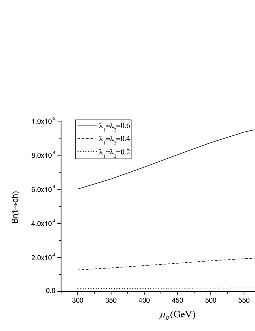
Figure 5: The branching ratio of t → c h → 𝑡 𝑐 ℎ t\rightarrow ch μ B subscript 𝜇 𝐵 \mu_{B}
We assume m Q ~ 4 = 790 G e V , m Z B = 1 T e V , λ Q = 0.5 , A B Q = 1 T e V formulae-sequence subscript 𝑚 subscript ~ 𝑄 4 790 G e V formulae-sequence subscript 𝑚 subscript 𝑍 𝐵 1 T e V formulae-sequence subscript 𝜆 𝑄 0.5 subscript 𝐴 𝐵 𝑄 1 T e V m_{\tilde{Q}_{4}}=790{\rm{GeV}},{m_{{Z_{B}}}}=1{\rm{TeV}},{\lambda_{Q}}=0.5,A_{BQ}=1{\rm{TeV}} t → c h → 𝑡 𝑐 ℎ t\rightarrow ch μ B subscript 𝜇 𝐵 \mu_{B} λ 1 = λ 2 = 0.6 , 0.4 , 0.2 formulae-sequence subscript 𝜆 1 subscript 𝜆 2 0.6 0.4 0.2
\lambda_{1}=\lambda_{2}=0.6,0.4,0.2 μ B subscript 𝜇 𝐵 {\mu_{B}} μ B subscript 𝜇 𝐵 \mu_{B}
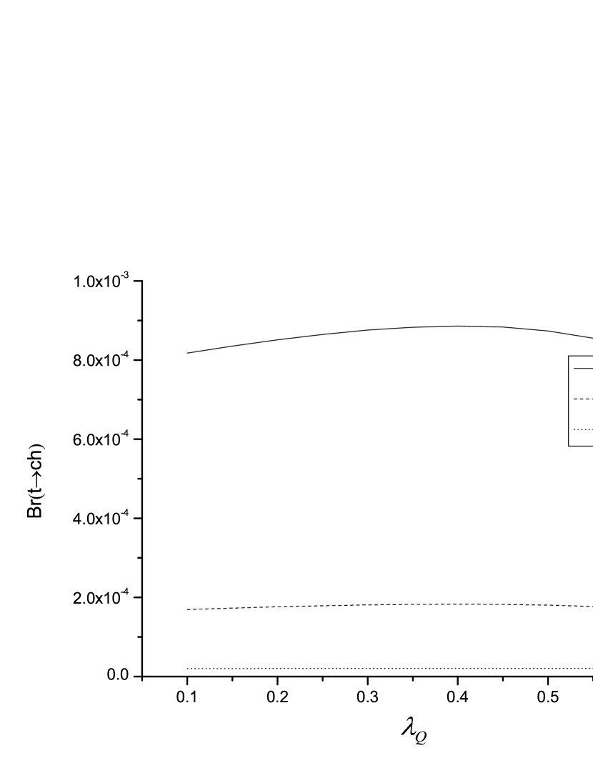
Figure 6: The branching ratio of t → c h → 𝑡 𝑐 ℎ t\rightarrow ch λ Q subscript 𝜆 𝑄 \lambda_{Q}
Choosing m Q ~ 4 = 790 G e V , m Z B = 1 T e V , μ B = 500 G e V , A B Q = 1 T e V formulae-sequence subscript 𝑚 subscript ~ 𝑄 4 790 G e V formulae-sequence subscript 𝑚 subscript 𝑍 𝐵 1 T e V formulae-sequence subscript 𝜇 𝐵 500 G e V subscript 𝐴 𝐵 𝑄 1 T e V {m_{{{\tilde{Q}}_{4}}}}=790{\rm{GeV}},{m_{{Z_{B}}}}=1{\rm{TeV}},{\mu_{B}}=500{\rm{GeV}},A_{BQ}=1{\rm{TeV}} ( t → c h ) → 𝑡 𝑐 ℎ (t\rightarrow ch) λ Q subscript 𝜆 𝑄 \lambda_{Q} λ 1 = λ 2 = 0.6 , 0.4 , 0.2 formulae-sequence subscript 𝜆 1 subscript 𝜆 2 0.6 0.4 0.2
\lambda_{1}=\lambda_{2}=0.6,0.4,0.2 λ Q subscript 𝜆 𝑄 \lambda_{Q}
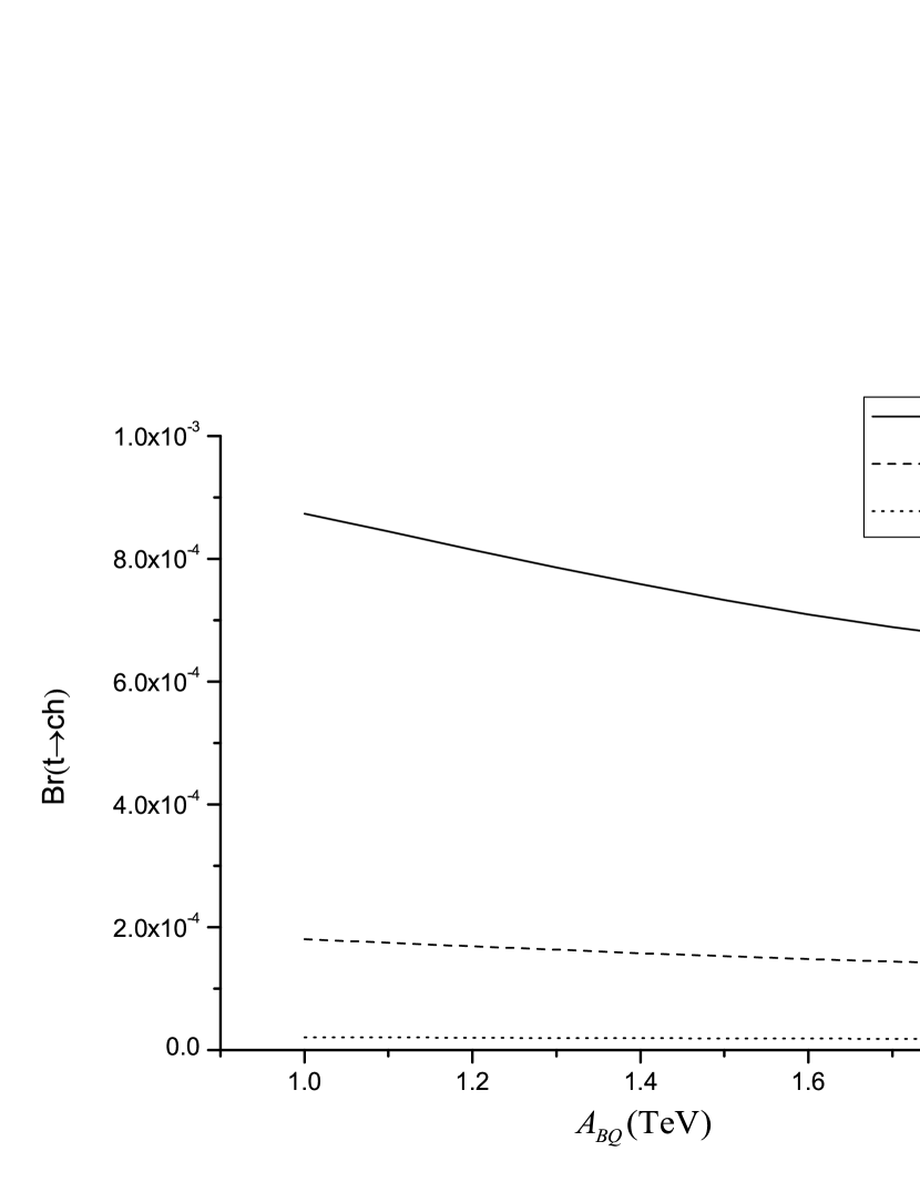
Figure 7: The branching ratio of t → c h → 𝑡 𝑐 ℎ t\rightarrow ch A B Q subscript 𝐴 𝐵 𝑄 A_{BQ}
Taking m Q ~ 4 = 790 G e V , m Z B = 1 T e V , μ B = 500 G e V , λ Q = 0.5 formulae-sequence subscript 𝑚 subscript ~ 𝑄 4 790 G e V formulae-sequence subscript 𝑚 subscript 𝑍 𝐵 1 T e V formulae-sequence subscript 𝜇 𝐵 500 G e V subscript 𝜆 𝑄 0.5 {m_{{{\tilde{Q}}_{4}}}}=790{\rm{GeV}},{m_{{Z_{B}}}}=1{\rm{TeV}},{\mu_{B}}=500{\rm{GeV}},{\lambda_{Q}}=0.5 ( t → c h ) → 𝑡 𝑐 ℎ (t\rightarrow ch) A B Q subscript 𝐴 𝐵 𝑄 A_{BQ} λ 1 = λ 2 = 0.6 subscript 𝜆 1 subscript 𝜆 2 0.6 \lambda_{1}=\lambda_{2}=0.6 λ 1 = λ 2 = 0.4 subscript 𝜆 1 subscript 𝜆 2 0.4 \lambda_{1}=\lambda_{2}=0.4 λ 1 = λ 2 = 0.2 subscript 𝜆 1 subscript 𝜆 2 0.2 \lambda_{1}=\lambda_{2}=0.2 A B Q subscript 𝐴 𝐵 𝑄 A_{BQ} A B Q subscript 𝐴 𝐵 𝑄 A_{BQ} λ 1 = λ 2 = 0.6 , 0.4 formulae-sequence subscript 𝜆 1 subscript 𝜆 2 0.6 0.4 \lambda_{1}=\lambda_{2}=0.6,0.4 ( t → c h ) → 𝑡 𝑐 ℎ (t\rightarrow ch) 10 − 4 superscript 10 4 10^{-4} λ 1 = λ 2 = 0.2 subscript 𝜆 1 subscript 𝜆 2 0.2 \lambda_{1}=\lambda_{2}=0.2 ( t → c h ) → 𝑡 𝑐 ℎ (t\rightarrow ch) 10 − 5 superscript 10 5 10^{-5}
V Summary
The running LHC is a top-quark factory, and provides a great
opportunity to seek out top-quark decays. And it is showed that the channel t → c h → 𝑡 𝑐 ℎ t\rightarrow ch ( t → c h ) ∼ 5 × 10 − 5 similar-to → 𝑡 𝑐 ℎ 5 superscript 10 5 (t\rightarrow ch)\sim 5\times 10^{-5} ref14 ; ref15 ref6 Br ( t → ch ) ∼ 10 − 13 similar-to Br → t ch superscript 10 13 \rm{Br}(t\rightarrow ch)\sim 10^{-13}
In this work, we study the rare top decay to a 125GeV Higgs in the framework of the BLMSSM.
Adopting reasonable assumptions on the parameter space, we present the radiative
correction to the process in BLMSSM, and draw some curves between the BRs and new physics parameters.
We get the branching ratio of t → c h → 𝑡 𝑐 ℎ t\rightarrow ch 10 − 3 superscript 10 3 10^{-3}
In addition, the author of ref16 ( t → c h ) < 2.7 % → 𝑡 𝑐 ℎ percent 2.7 (t\rightarrow ch)<2.7\% ( t → c h ) < 0.83 % → 𝑡 𝑐 ℎ percent 0.83 (t\rightarrow ch)<0.83\% 95 % percent 95 95\% t → c h → 𝑡 𝑐 ℎ t\rightarrow ch h → γ γ → ℎ 𝛾 𝛾 h\rightarrow\gamma\gamma t ¯ t ¯ 𝑡 𝑡 \bar{t}t ref17 ; ref18 λ 1 , 2 subscript 𝜆 1 2
\lambda_{1,2} ( t → c h ) → 𝑡 𝑐 ℎ (t\rightarrow ch) λ 1 , 2 subscript 𝜆 1 2
\lambda_{1,2}
As we could see above, the t → c h → 𝑡 𝑐 ℎ t\rightarrow ch
Acknowledgements.
The work has been supported by the National Natural Science Foundation of China (NNSFC)
with Grant No. 11275036, No. 11047002, the open project of State Key Laboratory of
Mathematics-Mechanization with Grant No. Y3KF311CJ1, the Natural Science Foundation of Hebei province with Grant No. A2013201277, and Natural Science Fund of Hebei
University with Grant No. 2011JQ05, No. 2012-242.