The static and dynamic polarisability, and the Stark and black-body radiation frequency shifts of the molecular hydrogen ions H${}_{2}^{+}$, HD⁺, and D${}_{2}^{+}$

Abstract

We calculate the DC Stark effect for three molecular hydrogen ions in the non-relativistic approximation. The effect is calculated both in dependence on the rovibrational state and in dependence on the hyperfine state. We discuss special cases and approximations. We also calculate the AC polarisabilities for several rovibrational levels, and therefrom evaluate accurately the black-body radiation shift, including the effects of excited electronic states. The results enable the detailed evaluation of certain systematic shifts of the transitions frequencies for the purpose of ultra-high-precision optical, microwave or radio-frequency spectroscopy in ion traps.

I Introduction

The molecular hydrogen ions represent a family of simple quantum systems that are amenable both to high-precision ab-initio calculations Gremaud98 ; Korobov Hilico Karr 2014 and to high-precision spectroscopy. Therefore, they are of great interest for the determination of fundamental constants Schiller 2007 , for tests of the time- and gravitational-potential-independence of fundamental constants SS1 ; SS2 , and for tests of QED Korobov Hilico Karr 2014 . On the experimental side, after early pioneering work on uncooled trapped ions and ions beams Jefferts ; Wing ; Carrington , the sympathetic cooling of trapped molecular hydrogen ions Schiller03 ; Blythe 2005 has opened up the window for high-precision radio-frequency, rotational, and rovibrational spectroscopy. Precision infrared laser spectroscopy of two rovibrational transitions has been achieved Schiller 2007 ; Bressel 2012 , and the fundamental rotational transition has also been observed Shen .

Because of the advances in experimental accuracy, and in order to open perspectives for future work directions, it has become important to evaluate the systematic effects on the transition frequencies. It is an advantage of the molecular hydrogen ion family that the sensitivities to external fields can be calculated ab-initio. The systematic effects treated so far include the Zeeman shift Zee1 ; Zee2 ; Karr Korobov Hilico Zeeman effect in H2+ , the electric quadrupole shift Bakalov and Schiller 2013 , and the black-body radiation (BBR) shift kool . The electric polarisability of the rovibrational levels of the molecular hydrogen ions has been of interest for a long time. It was computed with high accuracy for a subset of levels by several authors, in particular Bishop and Lam 1988 ; Bhatia-1 ; Hilico 2001 ; moss ; Yan ; Karr Kilic Hilico 2005 . These calculations used adiabatic or non-adiabatic wave functions. Ref. Hilico 2001 reviews the experimental and theoretical values for the ground state of $\hbox{\rm H}_{2}^{+}$ and $\hbox{\rm D}_{2}^{+}$. A particularly accurate calculation of the polarisability of $\hbox{\rm H}_{2}^{+}$ in its ground state was performed by one of the present authors, by including the relativistic corrections KorPRA00 . The dependence of the polarisability on the hyperfine state has only recently been obtained hfi , for the case of $\hbox{\rm HD}^{+}$, and it was shown that the dependence is very significant. These results have permitted a first analysis of the potential for ultra-high accuracy spectroscopy of $\hbox{\rm HD}^{+}$ and its suitability as an optical clock Bakalov and Schiller 2013 ; Schiller Bakalov Korobov PRL 2014 .

In the present paper, extensive calculations of the polarisability are presented. Its dependence on the hyperfine state is derived in a more elegant way and discussed in depth, both for $\hbox{\rm HD}^{+}$ and $\hbox{\rm H}_{2}^{+}$, since it is of great relevance for experiments.

While the BBR shift is tiny, it will eventually become of relevance for experiments requiring the highest levels of accuracy, such as the mentioned test of time-independence of fundamental constants. Therefore, this shift is also computed in detail. Results for $\hbox{\rm H}_{2}^{+}$ are presented for the first time. In addition, the case of $\hbox{\rm HD}^{+}$ is treated extensively, in view of the current experimental interest in this molecule.

This paper is structured as follows: In Sec. 2 we briefly review the calculation approach for the polarisability of the molecular hydrogen ions, neglecting spin effects. We define the effective Hamiltonian and present the tables of polarisabilities. In Sec. 3 we introduce the hyperfine structure and discuss the computation of the DC Stark shift in dependence of the spin state. We also give a number of useful approximations. Sec. 4 presents detailed results for a large number of hyperfine states potentially relevant for high-precision spectroscopy. In Sec. 5 we discuss the energy level shifts induced by the oscillating (AC) electric field of the black-body radiation, which we accurately evaluate by taking into account the precise frequency dependence of the polarisability.

II Evaluation of the polarisability

II.1 Non-relativistic polarisability. Spin-independent spatial considerations

For the purposes of evaluating the systematic effects in spectroscopy, it is at present sufficient to use the non-relativistic approximation to the polarisability. Therefore, we start from the non-relativistic Schrödinger equation:

$$(H_{0}-E)\Psi_{0}=0,\qquad H_{0}=-\frac{1}{2M_{1}}\mbox{$\nabla$}_{1}^{2}-\frac{1}{2M_{2}}\mbox{$\nabla$}_{2}^{2}-\frac{1}{2m_{e}}\mbox{$\nabla$}^{2}+\frac{1}{R}-\frac{1}{r_{1}}-\frac{1}{r_{2}},$$ (1)

where $M_{1}$ and $M_{2}$ are the masses of the nuclei (proton or deuteron), $R$ is the internuclear distance, $r_{1}$ and $r_{2}$ are the distances from nuclei 1 and 2 to the electron, respectively. The state $\Psi_{0}=|v\,L\rangle$ is the unperturbed state characterized by the vibrational and rotational quantum numbers $v,\,L$, and $E_{0}$ is its energy.

The interaction with an external electric field ${\bf E}$ in the dipole interaction form is expressed by

$$V_{p}=-\mathbf{E}\cdot{\bf d},\qquad{\bf d}=e\left[Z(\mathbf{R}_{1}+\mathbf{R}_{2})-\mathbf{r}\right]\,,$$ (2)

where $\mathbf{d}$ is the electric dipole moment of the three-particle-system, ${\bf R}_{1,2}$ and $\mathbf{r}$ are the position vectors of the nuclei and of the electron with respect to the center of mass.

Since the static or quasi-static electric fields present in an ion trap, and also the electric field of the radiation from continuous-wave lasers and from the black-body environmental radiation are typically weak, it is sufficient to apply second-order perturbation theory for the calculation of the polarisability. The energy shifts that result are typically at the level of 1 Hz, orders of magnitude smaller than the rotational or hyperfine splittings. For effects of higher-order in the external electric field, see Ref. Bhatia-1 .

The change of energy due to the polarisability of a molecular ion is expressed by

$$E_{p}^{(2)} = \langle\Psi_{0}|V_{p}(E_{0}-H_{0})^{-1}V_{p}|\Psi_{0}\rangle$$

$$= E^{i}E^{j}\langle\Psi_{0}|d^{i}(E_{0}-H_{0})^{-1}d^{j}|\Psi_{0}\rangle$$

$$= -\frac{1}{2}\alpha_{d}^{ij}E^{i}E^{j}\,,$$

where $\alpha_{d}^{ij}$, the polarisability tensor of rank 2, has been introduced,

$$\alpha_{d}^{ij}=-2\langle\Psi_{0}|d^{i}(E_{0}-H_{0})^{-1}d^{j}|\Psi_{0}\rangle.$$ (4)

The static dipole polarisability tensor is then reduced to scalar, $\alpha_{s}$, and tensor, $\alpha_{t}$, terms, which may be expressed in terms of three contributions corresponding to the possible values of of the rotational angular momentum quantum number of the intermediate state: $L^{\prime}=L\pm 1$, or $L^{\prime}=L$.

$$a_{+} = \;\;\frac{2}{2L+1}\sum_{p}\frac{\langle v\,L\|\mathbf{d}\|p\,(L+1)\rangle\langle p\,(L+1)\|\mathbf{d}\|v\,L\rangle}{E_{0}-E_{p}}\,,$$

$$a_{\text{0}} = -\frac{2}{2L+1}\sum_{p}\frac{\langle v\,L\|\mathbf{d}\|p\,L\rangle\langle p\,L\|\mathbf{d}\|v\,L\rangle}{E_{0}-E_{p}}\,,$$

$$a_{-} = \;\;\frac{2}{2L+1}\sum_{p}\frac{\langle v\,L\|\mathbf{d}\|p\,(L-1)\rangle\langle p\,(L-1)\|\mathbf{d}\|v\,L\rangle}{E_{0}-E_{p}}\,,$$ (5)

where $L$ is the rotational quantum number of the state under consideration, $E_{p}$ is the non-relativistic energy of the intermediate state $|p\,L^{\prime}\rangle$.

The polarisability tensor may be expressed as

$$\alpha_{d}^{ij}=\delta_{ij}\alpha_{s}+\alpha_{t}\left\langle\Psi_{0}|L_{i}L_{j}+L_{j}L_{i}-\frac{2}{3}\delta_{ij}\mathbf{L}^{2}|\Psi_{0}\right\rangle\,,$$ (6)

where $L_{i}$ are the Cartesian components of the rotational angular momentum operator, $\mathbf{L}^{2}=L_{x}^{2}+L_{y}^{2}+L_{z}^{2}$, and

$$\alpha_{s} = \frac{1}{3}(a_{+}+a_{0}+a_{-}),$$

$$\alpha_{t} = -\frac{a_{+}}{2(L+1)(2L+3)}+\frac{a_{0}}{2L(L+1)}-\frac{a_{-}}{2L(2L-1)}\,.$$

We may also define longitudinal ($\alpha_{\parallel}$) and transverse ($\alpha_{\bot}$) polarisabilities

$$\alpha_{\parallel} =\alpha_{s}+\alpha_{t}\left\langle\Psi_{0}|2\,L_{z}^{2}-\frac{2}{3}\mathbf{L}^{2}|\Psi_{0}\right\rangle$$ (7)

$$\alpha_{\bot} =\frac{1}{2}(\alpha_{d}^{xx}+\alpha_{d}^{yy})=\alpha_{s}+\alpha_{t}\left\langle\Psi_{0}|L_{x}^{2}+L_{y}^{2}-\frac{2}{3}\mathbf{L}^{2}|\Psi_{0}\right\rangle=\alpha_{s}-\frac{1}{2}\alpha_{t}\left\langle\Psi_{0}|2\,L_{z}^{2}-\frac{2}{3}\mathbf{L}^{2}|\Psi_{0}\right\rangle.$$ (8)

The definition of $\alpha_{\perp}$ as given above is reasonable, since axial symmetry requires that the matrix elements of $L_{x}^{2}$ and of $L_{y}^{2}$ are equal. Thus, the polarisabilities $\alpha_{\parallel}$ and $\alpha_{\perp}$ actually involve the expectation value of only a single operator, which has an alternative representation as the 0-component of the rank-2 tensor $\{{\bf L}\otimes{\bf L}\}_{2}$,

$$2\,L_{z}^{2}-\frac{2}{3}\mathbf{L}^{2}=\sqrt{\frac{8}{3}}\{{\bf L}\otimes{\bf L}\}_{20}\,.$$ (9)

In Sec. III, we will evaluate the polarisabilities of the hyperfine states of a given ro-vibrational level. The approximation we will use consists in introducing the polarisability operator, which holds in a manifold of given $L$,

$$\hat{\alpha}_{d}^{ij}(v,\,L) = \alpha_{s}(v,\,L)+\alpha_{t}(v,\,L)\left[L_{i}L_{j}+L_{j}L_{i}-\frac{2}{3}\delta_{ij}\mathbf{L}^{2}\right]\,,$$

$$\hat{\alpha}_{\parallel}(v,\,L) = \alpha_{s}(v,\,L)+\alpha_{t}(v,\,L)\sqrt{\frac{8}{3}}\{{\bf L}\otimes{\bf L}\}_{20}\,,$$

$$\hat{\alpha}_{\perp}(v,\,L) = \alpha_{s}(v,\,L)-\frac{1}{2}\alpha_{t}(v,\,L)\sqrt{\frac{8}{3}}\{{\bf L}\otimes{\bf L}\}_{20}\,.$$

Here, we have included the explicit dependence of the coefficients $\alpha_{s}$, $\alpha_{t}$ on the vibrational and rotational quantum numbers $v,\,L$. In the following, we will explicitly consider the polarisability anisotropy operator,

$$\hat{\alpha}_{\parallel}-\hat{\alpha}_{\perp}=\alpha_{t}(v,\,L)\,\frac{3}{2}\,\sqrt{\frac{8}{3}}\{{\bf L}\otimes{\bf L}\}_{20}=3\alpha_{t}(v,\,L)\left(L_{z}^{2}-\frac{1}{3}\mathbf{L}^{2}\right)\,.$$ (10)

II.2 Numerical results

Wave functions of the rovibrational states in the molecular hydrogen ions are obtained by using the variational approach expounded in Ref. KorPRA00 . Briefly, the wave function for a state with a total orbital angular momentum $L$ and of a total spatial parity $\pi=(-1)^{L}$ is expanded as follows:

$$\Psi_{LM}^{\pi}(\mathbf{R},\mathbf{r}_{1}) = \sum_{l_{1}+l_{2}=L}\mathcal{Y}_{LM}^{l_{1}l_{2}}(\hat{\mathbf{R}},\hat{\mathbf{r}}_{1})G_{l_{1}l_{2}}^{L\pi}(R,r_{1},r_{2}),$$

$$G_{l_{1}l_{2}}^{L\pi}(R,r_{1},r_{2}) = \sum_{n=1}^{N}\Big{\{}C_{n}\,\mbox{Re}\bigl{[}e^{-\alpha_{n}R-\beta_{n}r_{1}-\gamma_{n}r_{2}}\bigr{]}+$$ (11)

$$\,\,\,\,\,\,\,D_{n}\,\mbox{Im}\bigl{[}e^{-\alpha_{n}R-\beta_{n}r_{1}-\gamma_{n}r_{2}}\bigr{]}\Big{\}}\,,$$

where the complex exponents $\alpha$, $\beta$, $\gamma$, are generated in a pseudo-random way. The use of complex exponents instead of real ones allows reproducing the oscillatory behavior of the vibrational part of the wave function and improves the convergence rate. In numerical calculations we utilize basis sets as large as $N$ = 7 000 functions , in order to provide the required accuracy for the static polarisability of about 8 significant digits.

We note that a variational principle holds for the numerical value for $\alpha_{s}$ (but not for $\alpha_{t}$): the larger the value, the closer it is to the exact (non-relativistic) value, provided that the initial wave function is accurate enough.

The results of numerical calculations of the polarisabilities for a wide range of ro-vibrational states are presented in Tables 1, 2, 3. These polarisabilities do not include relativistic corrections. These have so far been computed only for the ground rovibrational level $(v=0,\,L=0)$ of $\hbox{\rm H}_{2}^{+}$ KorPRA00 . Therefore, the relative inaccuracy of the values of the table as compared to the exact values is of order $\alpha^{-2}\simeq 1\times 10^{-4}$. This is sufficiently small for current and near-future purposes.

Table 1: Polarisabilities of the $\mbox{HD}^{+}$ molecular ion, in atomic units.

$L=0$ $L=1$ $L=2$ $L=3$ $L=4$ $L=5$ $v$ $\alpha_{s}$ $\alpha_{s}~{}$ $\alpha_{t}$ $\alpha_{s}~{}$ $\alpha_{t}$ $\alpha_{s}~{}$ $\alpha_{t}~{}$ $\alpha_{s}~{}$ $\alpha_{t}$ $\alpha_{s}~{}$ $\alpha_{t}$ 0 395.30633 3.99015 175.48275 4.00956 13.82797 4.03878 3.19075 4.07794 1.10141 4.12721 0.47319 1 462.65271 4.70314 205.20067 4.72694 16.14340 4.76278 3.71557 4.81084 1.27799 4.87136 0.54642 2 540.68636 5.56925 239.58035 5.59871 18.81611 5.64313 4.31921 5.70273 1.48001 5.77786 0.62955 3 631.40288 6.63284 279.47585 6.66965 21.91000 6.72541 5.01516 6.80017 1.71152 6.89451 0.72396 4 737.31802 7.95478 325.95893 8.00132 25.50477 8.07195 5.82011 8.16691 1.97742 8.28690 0.83127 5 861.64968 9.61839 380.39514 9.67856 29.70139 9.76943 6.75494 9.89175 2.28374 10.04654 0.95337 6 1008.5802 11.74323 444.54814 11.82178 34.62944 11.94052 7.84610 12.10056 2.63789 12.30342 1.09241 7 1183.6432 14.50032 520.73882 14.60466 40.45801 14.76254 9.12757 14.97563 3.04910 15.24624 1.25088 8 1394.3075 18.14238 612.07821 18.28368 47.41173 18.49776 10.64364 18.78717 3.52889 19.15548 1.43147 9 1650.8846 23.05215 722.82833 23.24788 55.79504 23.54473 12.45301 23.94684 4.09171 24.45984 1.63690 10 1967.9875 29.82774 858.97404 30.10584 66.03006 30.52844 14.63477 31.10210 4.75562 31.83608 1.86935

Table 2: Polarisabilities of the $\mbox{H}_{2}^{+}$ molecular ion, in atomic units.

$L=0$ $L=1$ $L=2$ $L=3$ $L=4$ $L=5$ $v$ $\alpha_{s}$ $\alpha_{s}$ $\alpha_{t}$ $\alpha_{s}$ $\alpha_{t}$ $\alpha_{s}$ $\alpha_{t}$ $\alpha_{s}$ $\alpha_{t}$ $\alpha_{s}$ $\alpha_{t}$ 0 3.1687258 3.1783035 -0.8033729 3.1975081 -0.1931423 3.2264392 -0.0914467 3.2652493 -0.0544769 3.3141473 -0.0367142 1 3.8975634 3.9101018 -1.1442051 3.9352574 -0.2751013 3.9731892 -0.1302653 4.0241411 -0.0776138 4.0884471 -0.0523179 2 4.8215004 4.8380889 -1.6000689 4.8713900 -0.3847653 4.9216560 -0.1822373 4.9892726 -0.1086157 5.0747693 -0.0732474 3 6.0093275 6.0315483 -2.2129563 6.0761862 -0.5322759 6.1436389 -0.2521973 6.2345166 -0.1503892 6.3496578 -0.1014845 4 7.5604532 7.5906530 -3.0434869 7.6513642 -0.7322875 7.7432180 -0.3471422 7.8671844 -0.2071498 8.0246002 -0.1399110 5 9.6217735 9.6635170 -4.1811566 9.7475033 -1.0064626 9.8747452 -0.4774336 10.046804 -0.2851555 10.265837 -0.1928182 6 12.416000 12.474853 -5.7615823 12.593371 -1.3876723 12.773211 -0.6588274 13.016932 -0.3939491 13.328069 -0.2667729 7 16.290999 16.375936 -7.9965515 16.547168 -1.9273337 16.807463 -0.9160304 17.161118 -0.5485440 17.614095 -0.3721509 8 21.809473 21.935532 -11.228720 22.189990 -2.7087984 22.577626 -1.2892120 23.105870 -0.7734466 23.785138 -0.5259729 9 29.920328 30.113886 -16.036300 30.505195 -3.8730473 31.102847 -1.8465559 31.920266 -1.1104555 32.976407 -0.7574477 10 42.306330 42.616316 -23.445884 43.244200 -5.6711124 44.206257 -2.7100058 45.528094 -1.6347702 47.246181 -1.1195247

Table 3: Polarisabilities of the $\mbox{D}_{2}^{+}$ molecular ion, in atomic units.

$L=0$ $L=1$ $L=2$ $L=3$ $L=4$ $L=5$ $v$ $\alpha_{s}$ $\alpha_{s}$ $\alpha_{t}$ $\alpha_{s}$ $\alpha_{t}$ $\alpha_{s}$ $\alpha_{t}$ $\alpha_{s}$ $\alpha_{t}$ $\alpha_{s}$ $\alpha_{t}$ 0 3.0719887 3.0765904 -0.7579521 3.0858052 -0.1813435 3.0996560 -0.0852443 3.1181777 -0.0503016 3.1414173 -0.0335048 1 3.5530258 3.5585822 -0.9782731 3.5697111 -0.2340592 3.5864444 -0.1100266 3.6088309 -0.0649271 3.6369364 -0.0432481 2 4.1195817 4.1263238 -1.2485988 4.1398301 -0.2987476 4.1601453 -0.1404432 4.1873367 -0.0828824 4.2214959 -0.0552137 3 4.7912827 4.7995087 -1.5808716 4.8159913 -0.3782716 4.8407920 -0.1778439 4.8740043 -0.1049671 4.9157545 -0.0699367 4 5.5933149 5.6034134 -1.9904009 5.6236531 -0.4763025 5.6541185 -0.2239603 5.6949390 -0.1322078 5.7462891 -0.0881048 5 6.5583187 6.5708021 -2.4970077 6.5958274 -0.5975951 6.6335113 -0.2810366 6.6840342 -0.1659357 6.7476365 -0.1106108 6 7.7290547 7.7446049 -3.1266348 7.7757864 -0.7483752 7.8227607 -0.3520126 7.8857801 -0.2078964 7.9651778 -0.1386263 7 9.1622096 9.1817469 -3.9136471 9.2209342 -0.9368936 9.2799934 -0.4407873 9.3592871 -0.2604068 9.4592730 -0.1737083 8 10.933925 10.958708 -4.9041723 11.008431 -1.1742306 11.083398 -0.5526002 11.184144 -0.3265836 11.311297 -0.2179539 9 13.147977 13.179752 -6.1610454 13.243527 -1.4754879 13.339760 -0.6946003 13.469145 -0.4106838 13.632624 -0.2742310 10 15.948121 15.989359 -7.7712809 16.072159 -1.8615919 16.197178 -0.8766990 16.365416 -0.5186172 16.578236 -0.3465280

II.3 Scaling with rotational angular momentum

For large $L$, we find for $\hbox{\rm HD}^{+}$,

$$\alpha_{t}(v,\,L)\varpropto\frac{1}{L(L+1)(2L-1)(2L+3)}\,.$$ (12)

This follows from an argument described below after Eq. (25).

We have found heuristically, that for $\hbox{\rm H}_{2}^{+}$ and $\hbox{\rm D}_{2}^{+}$,

$$\alpha_{t}(v,\,L)\varpropto\frac{1}{(2L-1)(2L+3)}\,.$$ (13)

II.4 Comparison with previous work

II.4.1 Contribution from the ground electronic state

An approximation to the polarisability can be obtained using the well-known sum-over-intermediate-states expression, where the sum is truncated to a subset of levels. For $\hbox{\rm HD}^{+}$, such a calculation has been performed using transition dipole moments computed in the Born-Oppenheimer approximation hfi , including in the sum only levels of the ground electronic state (the inaccuracy of the used dipole moments is mentioned further below). At first sight, it may appear that the polarisability of a level $(v,\,L)$ in $\hbox{\rm HD}^{+}$ is dominated by the contribution from the rotational levels adjacent in energy to the particular state, namely $(v,\,L\pm 1)$. This is evidently true for $L=0$ levels. However, for $L\neq 0$, there is partial cancellation of the two contributions from $L^{\prime}=L\pm 1$. Even then, the $\alpha_{t}$ values indeed arise essentially from the rovibrational transitions. However, the $\alpha_{s}(L>0)$ values are actually dominated by the contribution from the excited electronic states. The comparison of the accurate results given in the tables above with the truncated-sum results allows putting in evidence the contribution from the excited electronic states. The comparison is shown in Table 4, showing that for low-lying rovibrational levels ($v,\,L<5)$, the difference is of order several atomic units for $\alpha_{s}$ and less than 2.5 atomic units for $\alpha_{t}$. The increase of the difference with $v$ is due to the fact that the contributions from excited electronic states become more important since the level $v$ is getting closer in energy to them.

$\begin{array}[]{|c|c|cc|cc|cc|cc|}\hline\cr\text{$v$}&L=0&L=1&&L=2&&L=3&&L=4&\\ \hline\cr\text{}&\delta\alpha_{s}&\delta\alpha_{s}&\delta\alpha_{t}&\delta\alpha_{s}&\delta\alpha_{t}&\delta\alpha_{s}&\delta\alpha_{t}&\delta\alpha_{s}&\delta\alpha_{t}\\ \hline\cr 0&3.3&3.1&-0.72&3.1&-0.18&3.2&-0.08&3.2&-0.06\\ 1&3.9&3.7&-0.98&3.8&-0.24&3.8&-0.12&3.8&-0.08\\ 2&4.7&4.5&-1.34&4.5&-0.34&4.6&-0.16&4.6&-0.10\\ 3&5.6&5.4&-1.80&5.5&-0.44&5.5&-0.22&5.6&-0.12\\ 4&6.8&6.6&-2.42&6.6&-0.60&6.7&-0.28&6.8&-0.16\\ \hline\cr\end{array}$

Table 4: Difference $\delta\alpha$ between the accurate polarisabilities of $\hbox{\rm HD}^{+}$ (this work) and those computed by a summation over all intermediate rovibrational states in the ground electronic state, in atomic units. The latter are calculated from the results of Ref. hfi (which are there given in terms of $\alpha_{vLFSJJ_{z}}^{(l)},$ $\alpha_{vLFSJJ_{z}}^{(t)}$) as $\alpha_{s}(v,\,L)=(\alpha_{vLFSJJ_{z}}^{(l)}+2\alpha_{vLFSJJ_{z}}^{(t)})/3$ (where any hyperfine state $(F,\,S,\,J,\,J_{z})$ can be chosen) and $\alpha{}_{t}(v,\,L)=(\alpha_{vLn_{s}}^{(l)}-\alpha_{vLn_{s}}^{(t)})/L(2L-1)$, where $n_{s}$ denotes the stretched state, defined in Sec. III.3.3.

For the homonuclear $\hbox{\rm H}_{2}^{+}$ and $\hbox{\rm D}_{2}^{+}$ the polarisability arises only from the excited electronic states, since there is no electric-dipole coupling between levels of the ground electronic state. As a consequence, the polarisabilities $\alpha_{s}(L=0)$ and $\alpha_{t}(v,\,L)$ are much smaller than in the case of the heteronuclear ions, as has been noted in previous studies cited above.

II.4.2 General calculations

We can compare our results with some previous studies.

Early on, Bishop and Lam Bishop and Lam 1988 studied the states $v=0,\,L=0-10$ of $\hbox{\rm H}_{2}^{+}$. The largest number of levels was considered by Moss and Valenzano, who covered the three ion species also treated here, with $L=0,\,1$, and all $v$ moss . Our results agree with theirs, to within two units of the last digit reported by them, except for the level $(v=8,\,L=1)$, where the largest discrepancy occurs, 0.007 at. u.

The agreement with the $L=0$ values for the three ion species determined by Hilico et al. Hilico 2001 , and Karr et al. Karr Kilic Hilico 2005 is better than $4\times 10^{-8}$ in relative terms.

Pilon and Baye recently computed the polarisabilities of $\hbox{\rm H}_{2}^{+}$ for a number of levels Pilon and Baye . The values for $v=0,\,L=0,\,1,\,2,\,3,\,4,\,5$ agree to better than $2\times 10^{-8}$ in relative terms. For $L=1,\,v=0,\,1,\,2,\,3$ and for $L=2,\,v=0,\,1,\,2,\,3$ the values agree with the present values to better than $3\times 10^{-7}$ in relative terms.

III Perturbation theory for the hyperfine states

III.1 Energy shifts

The hyperfine interactions split each rovibrational level into a number of hyperfine sub-levels. We denote the corresponding kets as $|m\rangle=|v\,L\,n\,J_{z}\rangle$, where $n$ is a label for the particular hyperfine state in a rovibrational level $(v,\,L)$ (note that this notation includes both pure and non-pure spin states). $n$ is written as $(F,\,S,\,J)$ for $\hbox{\rm HD}^{+}$ and $(I,\,S,\,J)$ for $\hbox{\rm H}_{2}^{+}$, see Sec. III.2 below. When the Stark shifts of the quantum levels are small compared to other shifts, we can apply first-order perturbation theory. The Stark energy shift of a state $|m\rangle$ can be expressed in different ways (for simplicity, in the following we omit the caret on the polarization operators) Arosa presentation :

$$\Delta E(m) =-\frac{1}{2}\left[\langle m|\alpha_{\parallel}|m\rangle E_{z}^{2}+\langle m|\alpha_{\perp}|m\rangle(E_{x}^{2}+E_{y}^{2})\right]\,,$$

$$=-\frac{1}{2}\left[\alpha_{s}(E_{x}^{2}+E_{y}^{2}+E_{z}^{2})+\alpha_{t}(E_{z}^{2}-\frac{1}{2}(E_{x}^{2}+E_{y}^{2}))\langle m|\sqrt{\frac{8}{3}}\{{\bf L}\otimes{\bf L}\}_{20}|m\rangle\right]\,,$$

$$=-\frac{1}{2}\alpha_{s}(E_{x}^{2}+E_{y}^{2}+E_{z}^{2})-\alpha_{t}(E_{z}^{2}-\frac{1}{2}(E_{x}^{2}+E_{y}^{2}))\langle m|L_{z}^{2}-\frac{1}{3}{\bf L}^{2}|m\rangle\,,$$

$$=-\frac{1}{2}{\bf E}^{2}\left(\alpha_{s}+\alpha_{t}(3\cos^{2}\theta-1)\langle m|L_{z}^{2}-\frac{1}{3}{\bf L}^{2}|m\rangle\right)\,,$$

$$=-\frac{1}{2}{\bf E}^{2}\left(\alpha_{s}(v,\,L)+(3\cos^{2}\theta-1)\frac{1}{3}\langle v\,L\,n\,J_{z}|\alpha_{\parallel}-\alpha_{\perp}|v\,L\,n\,J_{z}\rangle\right)\,,$$ (14)

where $\theta$ is the angle between the quantization axis and the direction of the electric field ${\bf E}$.

In Refs. hfi ; Bakalov and Schiller 2013 the levels shifts were described in terms of longitudinal polarisability, $\alpha^{(l)}$, and transverse polarisability $\alpha^{(t)}$. They are related to the expectation values of the operators introduced here by $\langle m|\alpha_{\parallel}|m\rangle=\alpha^{(l)}$ and $\langle m|\alpha_{\perp}|m\rangle=\alpha^{(t)}$.

III.2 Hyperfine structure

We limit ourselves in the following to the ion species $\hbox{\rm H}_{2}^{+}$ and $\hbox{\rm HD}^{+}$, which are most relevant for experimental work at present.

In case of the molecular ion $\hbox{\rm H}_{2}^{+}$ we have identical nuclei and nuclear permutation symmetry. This makes some spin configurations forbidden and splits the consideration of hyperfine states into two cases (see KorPRA06R ): for even $L$, the total nuclear spin $I$ is zero and only two hyperfine sub-levels are possible; for states with odd $L$, the total nuclear spin is one and the ro-vibrational level is split into 5 or 6 hyperfine sub-levels, depending on the value of $L$.

The most suitable coupling scheme of angular momentum operators is

$$\mathbf{S}=\mathbf{I}+\mathbf{s}_{e},\qquad\mathbf{J}=\mathbf{S}+\mathbf{L\,},$$ (15)

where $\mathbf{I}$ is the total nuclear spin operator, and ${\bf s}_{e}$ is the electron spin operator. The basis states which correspond to this coupling are

$$|ISLJJ_{z}\rangle=\sum_{I_{z},\,\xi,\,S_{z}}C_{S\,S_{z},L\,L_{z}}^{J\,J_{z}}C_{I\,I_{z},s_{e}\xi}^{S\,S_{z}}\Bigl{(}|I\,I_{z}\rangle\cdot|s_{e}\xi\rangle\cdot|L\,L_{z}\rangle\Big{)}\,,$$ (16)

and will be called pure states Karr Bielsa et al 2008 .

The effective HFS Hamiltonian is expressed as KorPRA06R

$$\begin{array}[]{@{}l}{\displaystyle H_{{\rm eff}}=b_{F}(\mathbf{I}\cdot\mathbf{s}_{e})+c_{e}(\mathbf{L}\cdot\mathbf{s}_{e})+c_{I}(\mathbf{L}\cdot\mathbf{I})}\\[5.69054pt] {\displaystyle\hskip 28.45274pt+\frac{d_{1}}{(2L-1)(2L+3)}\biggl{\{}\frac{2}{3}\mathbf{L}^{2}(\mathbf{I}\cdot\mathbf{s}_{e})-\Bigl{[}(\mathbf{L}\cdot\mathbf{I})(\mathbf{L}\cdot\mathbf{s}_{e})+(\mathbf{L}\cdot\mathbf{s}_{e})(\mathbf{L}\cdot\mathbf{I})\Bigr{]}\biggr{\}}}\\[8.53581pt] {\displaystyle\hskip 28.45274pt+\frac{d_{2}}{(2L-1)(2L+3)}\left[\frac{1}{3}\mathbf{L}^{2}\mathbf{I}^{2}-\frac{1}{2}(\mathbf{L}\cdot\mathbf{I})-(\mathbf{L}\cdot\mathbf{I})^{2}\right].}\end{array}$$ (17)

For the case of even $L$, the pure states are the true HFS eigenstates, since the $2\!\times\!2$ effective HFS Hamiltonian matrix is diagonal. Even for odd-$L$ states, the pure states are good approximations to the true HFS states Karr Bielsa et al 2008 , since the coefficients of admixture of other states to a given true HFS state are small, e.g. for $L=1$ do not exceed 0.04, and for $L=3$ do not exceed 0.06. This means that even in this case, a good approximation for expectation values such as Eq. (14) may be obtained using the pure states.

For the hydrogen molecular ion $\hbox{\rm HD}^{+}$ the coupling scheme of the particle angular momentum operators is prl06

$$\mathbf{F}=\mathbf{I}_{p}+\mathbf{s}_{e},\quad\mathbf{S}=\mathbf{F}+\mathbf{I}_{d},\quad\mathbf{J}=\mathbf{S}+\mathbf{L}\,.$$ (18)

${\bf I}_{p},\,{\bf I}_{d}$ are the proton and deuteron spin operators, respectively. The effective Hamiltonian is given in Ref. prl06 . The pure states are determined in a similar way as in Eq. (16). In zero magnetic field, the pure states represent a good approximation to some of the true HFS states, and may be used to calculate approximate values of the polarisabilities. Details are given in Sec. IV below. Hyperfine states are labeled by $n=(F\,S\,J)$.

III.3 Analytical results

In this subsection we discuss some useful results that allow to understand several dependencies. In particular we discuss the polarisabilities of the pure spin states, for two reasons. First, a significant part of hyperfine states may be well approximated by pure spin states; second, since all hyperfine states can be expressed as weighted sums of pure spin states, their polarisabilities can conveniently be computed from the pure state polarisabilities.

III.3.1 Zero magnetic field

When the magnetic field is zero, the total angular momentum squared ${\bf J}^{2}$ commutes with the hyperfine Hamiltonian and $J$ is a good quantum number. Therefore we can apply the Wigner-Eckart theorem, and separate the $J_{z}$- dependence of the expectation value:

$$\langle vLnJ_{z}|\{{\bf L}\otimes{\bf L}\}_{20}|vLnJ_{z}\rangle = C_{20,JJ_{z}}^{JJ_{z}}\langle vLn||\{{\bf L}\otimes{\bf L}\}_{2}||vLn\rangle/\sqrt{2J+1}$$ (19)

$$= -\frac{J(J+1)-3J_{z}^{2}}{\sqrt{J(J+1)(2J-1)(2J+1)(2J+3)}}\langle vLn||\{{\bf L}\otimes{\bf L}\}_{2}||vLn\rangle$$

We therefore obtain the $J_{z}$ - dependence of the polarisability anisotropy as follows:

$$\langle vLnJ_{z}|\alpha_{\parallel}-\alpha_{\perp}|vLnJ_{z}\rangle=\left(1-\frac{3\,J_{z}^{2}}{J(J+1)}\right)\langle vLnJ_{z}=0|\alpha_{\parallel}-\alpha_{\perp}|vLnJ_{z}=0\rangle\,.$$ (20)

Note that this result holds both for pure and non-pure spin states. It follows that for $J=0$ states, the polarisability anisotropy is zero. For $\hbox{\rm HD}^{+}$, $J=0$ states can only occur for $L<3$, since the minimum $J$ value permitted by angular momentum algebra is $L-2$. For $\hbox{\rm H}_{2}^{+}$, there are no such states, since $J$ is a half-integer number.

III.3.2 Pure states

For pure angular momentum states, the matrix elements of the polarisability anisotropy can be evaluated explicitly. Considering only the coupling scheme $\mathbf{J}=\mathbf{S}+\mathbf{L}$, we have (note that this is independent of $I$ or $F$)

$$\begin{array}[]{@{}l}{\displaystyle\left\langle SLJJ_{z}\left|2\left(L_{z}^{2}-\frac{1}{3}\mathbf{L}^{2}\right)\right|SLJJ_{z}\right\rangle=\sqrt{\frac{8}{3}}\left\langle SLJJ_{z}|\{\mathbf{L}\otimes\mathbf{L}\}_{20}|SLJJ_{z}\right\rangle\,\,,}\\[11.38109pt] \hskip 28.45274pt{\displaystyle=\sqrt{\frac{8}{3}}\,\frac{C_{JJ_{z},20}^{JJ_{z}}}{\sqrt{2J+1}}\,\left\langle SLJ\|\{\mathbf{L}\otimes\mathbf{L}\}_{2}\|SLJ\right\rangle}\,\,,\\[11.38109pt] \hskip 28.45274pt{\displaystyle=-\frac{(J(J+1)-3J_{z}^{2})\,[3D(D-1)-4J(J+1)L(L+1)]}{3J(J+1)(2J-1)(2J+3)}}\,\,,\end{array}$$ (21)

where

$$D=J(J+1)+L(L+1)-S(S+1)\,.$$ (22)

This result is obtained using the following relations Messiah ; Varshalovich 1988

$$\begin{array}[]{@{}l}{\displaystyle\bigl{\langle}SLJ\bigl{\|}\{\mathbf{L}\otimes\mathbf{L}\}_{2}\bigr{\|}SLJ\bigr{\rangle}=(2J+1)(-1)^{S+L+J+2}\left\{\begin{matrix}L&\!L\!&2\\ J&\!J\!&S\end{matrix}\right\}\left\langle L\|\{\mathbf{L}\otimes\mathbf{L}\}_{2}\|L\right\rangle\,,}\\[8.53581pt] {\displaystyle\left\langle L\|\{\mathbf{L}\otimes\mathbf{L}\}_{2}\|L\right\rangle=\frac{1}{\sqrt{6}}\sqrt{L(L+1)}\sqrt{(2L-1)(2L+1)(2L+3)}}\,.\end{array}$$

In $\hbox{\rm H}_{2}^{+}$ we consider first the states having even $L$, so $I=0$. Then $S=1/2$. These pure states are exact HFS eigenstates, and therefore Eq. (21) immediately gives the exact Stark shift using Eqs. (14, 20):

$$\langle m({\rm even}\,L)|\alpha_{\parallel}-\alpha_{\perp}|m({\rm even}\,L)\rangle_{{\rm H_{2}^{+}}}=-\frac{3}{2}\alpha_{t}(v,\,L)\,\frac{(J(J+1)-3J_{z}^{2})\,[3D(D-1)-4J(J+1)L(L+1)]}{3J(J+1)(2J-1)(2J+3)}\,.$$ (23)

with $D=J(J+1)+L(L+1)-3/4$.

For pure states with odd $L$ (and therefore $I=1$):

$$\begin{array}[]{@{}l}\left\langle I=1\,S\,L\,J\Bigl{\|}\{\mathbf{L}\otimes\mathbf{L}\}_{2}\Bigr{\|}I=1\,S\,L\,J\right\rangle=(2J+1)(-1)^{S+L+J}\left\{\begin{matrix}L&\!L\!&2\\ J&\!J\!&S\end{matrix}\right\}\left\langle L\|\left\{\mathbf{L}\otimes\mathbf{L}\right\}_{2}\|L\right\rangle\\[8.53581pt] \hskip 28.45274pt{\displaystyle=\sqrt{\frac{2J+1}{6}}\,\frac{3D(D-1)-4J(J+1)L(L+1)}{2\sqrt{J(J+1)(2J-1)(2J+3)}}\,,}\end{array}$$ (24)

where $D$ is given by Eq. (22). We see that the actual value of $I$ does not occur on the r.h.s., and that we obtain the same result as for the $I=0$ pure states. Eq. (23) is an approximate result also for the odd-$L$ hyperfine states of $\hbox{\rm H}_{2}^{+}$ which are not pure, provided they are approximately pure (see below).

In the case of $\hbox{\rm HD}^{+}$, where the pure states are denoted as $|F\,S\,L\,J\,J_{z}\rangle$, Eq. (23) also holds, where $L$ now can be even or odd. There is no dependence on $F$.

Summarizing, for any pure state of $\hbox{\rm H}_{2}^{+}$ and $\hbox{\rm HD}^{+}$, and, by consequence, also for all other molecular hydrogen ions, Eq. (23) gives the polarisability anisotropy:

$$\langle{\rm pure\,state}|\alpha_{\parallel}-\alpha_{\perp}|{\rm pure\,state}\rangle_{\text{{\rm any species}}}=-\frac{3}{2}\alpha_{t}(v,\,L)\,\frac{(J(J+1)-3J_{z}^{2})\,[3D(D-1)-4J(J+1)L(L+1)]}{3J(J+1)(2J-1)(2J+3)}\,.$$ (25)

We note that Roeggen Roeggen has developed an approximate theory of the polarisability of heteronuclear diatomic molecules with spin, neglecting nuclear spin. If we combine our Eq. (25) and the approximate dependencies Eq. (12) we reproduce the result given in Eqs. (62, 63) of Ref. Roeggen .

III.3.3 The stretched states

The stretched states are those exact HFS states having maximal total angular momentum $J$ and maximal (absolute) projection $|J_{z}|$. These are also pure states. In $\hbox{\rm HD}^{+}$, these are the states $|v\,L\,n_{s}\rangle$, where $n_{s}$ denotes the stretched hyperfine state: $F=1,\,S=2,\,J=L+2,$ $J_{z}=\pm(L+2)$. We find from Eq. (23) or by analytical evaluation of the matrix elements for these two stretched states (the evaluation is simple, if the calculations is done with the basis functions being the eigenfunctions of the individual angular momenta $I_{p},\,I_{d},\,S,\,L$),

$$\langle v\,L\,n_{s}|\alpha_{\parallel}-\alpha_{\perp}|v\,L\,n_{s}\rangle=L(2L-1)\,\alpha_{t}(v,\,L)\,.$$ (26)

Compare the discussion in Ref. Bakalov and Schiller 2013 .

In $\hbox{\rm H}_{2}^{+}$, the stretched states are $|v\,L\,n_{s}\rangle\equiv|v,\,L,\,I=1,\,S=3/2,\,J=L+3/2,\,J_{z}=\pm(L+3/2)\text{$\rangle$}$. The same result Eq. (26) is obtained.

By evaluating the polarisabilities of all hyperfine states, we find that if $L>1$, the largest value of $\langle m|\alpha_{\parallel}-\alpha_{\perp}|m\rangle$ within a rovibrational level occurs for the stretched states (see tables below). Therefore, in the following discussion, we normalize the polarisability anisotropy values of any hyperfine state in a particular rovibrational level relative to that of the stretched states in that same level.

For $\hbox{\rm HD}^{+}$, combining the result Eq. (26) for the stretched states with the approximate behavior Eq. (12), we obtain $\langle v\,L\,n_{s}|\alpha_{\parallel}-\alpha_{\perp}|v\,L\,n_{s}\rangle\propto(3+5\,L+2\,L^{2})^{-1}$. This describes a rather strong decrease in the magnitude of all anisotropic polarisability values, not only those of the stretched-states, with increasing $L$.

IV Numerical results for the hyperfine-state dependence

The evaluation of the matrix elements of Eq. (10) for all (exact) hyperfine states is straightforward, once the hyperfine states in absence of electric field are known. The calculation can for example proceed by considering the expansion of the hyperfine states in pure states, and then applying Eq. (25), which holds for the pure states of any molecular hydrogen ion. Actually, the matrix elements are the same (apart from prefactors such as $\alpha_{t}$) as the matrix elements for the electric quadrupole shift evaluated in Ref. Bakalov and Schiller 2013 , and an explicit formula is given there.

We have performed the computation for the rovibrational levels up to $v=4$ and $L=4$. Note that the polarisability anisotropy vanishes for $L=0$ states and is therefore not reported in the tables. We confine ourselves to the case of zero magnetic field.

The results are summarized in table 5 and table 6 where we give the values for the hyperfine states having $J_{z}=0$. The values for $J_{z}\neq 0$ can be easily obtained using Eq. (20). Note that for a given hyperfine state and value of $L$ the dependence on $v$ is usually weak, limited to several percent, except for a few cases.

$\begin{array}[]{|l|c|c|c|c|c|c|}\hline\cr{\rm{\rm hyp.\,state}}&{\rm Eq.\,(}\ref{eq:anisotropic polarisability any pure state})&&&{\rm level}&&\\ \text{$(F,\,S,\,J,\,J_{z})$}&\text{(normalized)}&\text{$(v,L)=(0,1)$}&\text{$(v,L)=(1,1)$}&\text{$(v,L)=(2,1)$}&\text{$(v,L)=(3,1)$}&\text{$(v,L)=(4,1)$}\\ \hline\cr(0,1,2,0)&-1&-0.999422&-0.999457&-0.999491&-0.999525&-0.999558\\ (0,1,1,0)&1&0.998747&0.998825&0.998902&0.998978&0.999053\\ (0,1,0,0)*&0&0&0&0&0&0\\ (1,0,1,0)&-2&-1.66845&-1.69239&-1.71585&-1.73892&-1.76151\\ (1,1,1,0)&1&0.590503&0.619326&0.647628&0.675521&0.702883\\ (1,1,0,0)*&0&0&0&0&0&0\\ (1,1,2,0)&-1&-0.999973&-0.999972&-0.999971&-0.99997&-0.99997\\ (1,2,1,0)&-0.2&-0.120803&-0.125763&-0.130681&-0.135574&-0.140428\\ (1,2,3,0)*&-0.8&-0.8&-0.8&-0.8&-0.8&-0.8\\ (1,2,2,0)&1&0.999395&0.999429&0.999462&0.999495&0.999528\\ \hline\cr\end{array}$

Table 5: The normalized anisotropic polarisabilities for the $J_{z}=0$ - hyperfine states of $\hbox{\rm HD}^{+}$ in $L=1$ levels. The first column shows the hyperfine state’s label $n,\,J_{z}$ ($F$ and $S$ are usually approximate, $J$ is an exact quantum number), the second column contains the normalized values $\langle v\,L\,F\,S\,J\,J_{z}=0|\alpha_{\parallel}-\alpha_{\perp}|v\,L\,F\,S\,J\,J_{z}=0\rangle/\langle v\,L\,n_{s}|\alpha_{\parallel}-\alpha_{\perp}|v\,L\,n_{s}\rangle$ for the pure state $|v\,L\,F\,S\,J\,J_{z}=0\rangle$ giving the largest contribution to the exact HFS state $|v\,L\,n\,J_{z}=0\rangle$ (note that the values are independent of $F$ and of $v$). The following columns give the actual values $\langle v\,L\,n\,J_{z}=0|\alpha_{\parallel}-\alpha_{\perp}|v\,L\,n\,J_{z}=0\rangle/\langle v\,L\,n_{s}|\alpha_{\parallel}-\alpha_{\perp}|v\,L\,n_{s}\rangle$ for each hyperfine state. The normalization is with respect to the polarisability anisotropy of the stretched state $|v\,L\,n_{s}\rangle$ of the same rovibrational level. The three states marked with an asterisk are pure states.

$\begin{array}[]{|l|c|c|c|c|c|c|}\hline\cr{\rm hyp.\,state}&{\rm Eq.}\,(\ref{eq:anisotropic polarisability any pure state})&&&{\rm level}(v,L)&&\\ \text{$(F,\,S,\,J,\,J_{z})$}&\text{{\rm(normalized)}}&\text{$(v,L)=(0,2)$}&\text{$(v,L)=(1,2)$}&\text{$(v,L)=(2,2)$}&\text{$(v,L)=(3,2)$}&\text{$(v,L)=(4,2)$}\\ \hline\cr(0,1,3,0)&-0.8&-0.799487&-0.799517&-0.799548&-0.799578&-0.799608\\ (0,1,2,0)&-0.5&-0.499349&-0.49939&-0.49943&-0.499469&-0.499508\\ (0,1,1,0)&-0.7&-0.698944&-0.699011&-0.699076&-0.699141&-0.699205\\ (1,0,2,0)&-1&-0.89668&-0.902108&-0.907625&-0.913227&-0.918913\\ (1,1,1,0)&-0.7&-0.598522&-0.605382&-0.612152&-0.618825&-0.625393\\ (1,1,2,0)&-0.5&-0.572569&-0.56875&-0.564853&-0.560883&-0.556839\\ (1,1,3,0)&-0.8&-0.798847&-0.798904&-0.798961&-0.799019&-0.799079\\ (1,2,0,0)*&0&0&0&0&0&0\\ (1,2,1,0)&0.7&0.597466&0.604392&0.611229&0.617966&0.624598\\ (1,2,2,0)&0.2143&0.182884&0.184534&0.186194&0.187865&0.189546\\ (1,2,3,0)&-0.2&-0.201666&-0.201579&-0.201491&-0.201403&-0.201313\\ (1,2,4,0)*&-0.7143&-0.714286&-0.714286&-0.714286&-0.714286&-0.714286\\ \hline\cr\text{}&\text{}&\text{$(v,L)$=(0,3)}&\text{$(v,L)$=(1,3)}&\text{$(v,L)$=(2,3)}&\text{$(v,L)$=(3,3)}&\text{$(v,L)$=(4,3)}\\ \hline\cr(0,1,4,0)&-0.7143&-0.713807&-0.713835&-0.713864&-0.713892&-0.71392\\ (0,1,3,0)&-0.6&-0.599383&-0.599421&-0.599459&-0.599496&-0.599533\\ (0,1,2,0)&-0.6857&-0.684872&-0.684925&-0.684977&-0.685028&-0.685079\\ (1,0,3,0)&-0.8&-0.743487&-0.745805&-0.748206&-0.750693&-0.753272\\ (1,1,2,0)&-0.6857&-0.641563&-0.644157&-0.646756&-0.649358&-0.651959\\ (1,1,3,0)&-0.6&-0.638925&-0.637509&-0.636019&-0.634449&-0.632793\\ (1,1,4,0)&-0.7143&-0.712034&-0.712155&-0.712277&-0.712399&-0.712523\\ (1,2,1,0)*&-0.48&-0.48&-0.48&-0.48&-0.48&-0.48\\ (1,2,2,0)&-0.1714&-0.216421&-0.213776&-0.211124&-0.208471&-0.205819\\ (1,2,3,0)&-0.2533&-0.271538&-0.270598&-0.26965&-0.268696&-0.267735\\ (1,2,4,0)&-0.4286&-0.431302&-0.431152&-0.431002&-0.430852&-0.4307\\ (1,2,5,0)*&-0.6667&-0.666667&-0.666667&-0.666667&-0.666667&-0.666667\\ \hline\cr\text{}&\text{}&\text{$(v,L)$=(0,4)}&\text{$(v,L)$=(1,4)}&\text{$(v,L)$=(2,4)}&\text{$(v,L)$=(3,4)}&\text{$(v,L)$=(4,4)}\\ \hline\cr(0,1,5,0)&-0.6667&-0.666213&-0.66624&-0.666267&-0.666293&-0.66632\\ (0,1,4,0)&-0.6071&-0.606572&-0.606607&-0.606642&-0.606676&-0.60671\\ (0,1,3,0)&-0.6548&-0.654035&-0.654081&-0.654126&-0.65417&-0.654214\\ (1,0,4,0)&-0.7143&-0.677583&-0.678822&-0.68012&-0.68148&-0.682906\\ (1,1,3,0)&-0.6548&-0.627904&-0.62934&-0.630793&-0.632265&-0.633749\\ (1,1,4,0)&-0.6071&-0.630532&-0.629989&-0.62939&-0.628733&-0.628016\\ (1,2,2,0)*&-0.5612&-0.561224&-0.561224&-0.561224&-0.561224&-0.561224\\ (1,1,5,0)&-0.6667&-0.663695&-0.663856&-0.664019&-0.664183&-0.664348\\ (1,2,3,0)&-0.3929&-0.420442&-0.41896&-0.417462&-0.415946&-0.414418\\ (1,2,4,0)&-0.4096&-0.423439&-0.422708&-0.421974&-0.421236&-0.420494\\ (1,2,5,0)&-0.5&-0.503426&-0.503237&-0.503047&-0.502857&-0.502666\\ (1,2,6,0)*&-0.6364&-0.636364&-0.636364&-0.636364&-0.636364&-0.636364\\ \hline\cr\end{array}$

Table 6: Same as Table 5, but for levels $L=2,\,3,\,4$. Note that the values in the second column are rounded.

By looking at the values in the Tables 5, 6, one can see that the approximation that the polarisability does not depend on $F$ is quite good for some hyperfine states, and moderate in others, which is due to their more or less pure character. In order to obtain values accurate to better than one atomic unit for $\hbox{\rm HD}^{+}$, because of its large values of $\alpha_{t}$ it is necessary to use the exact hyperfine dependence of the polarisability anisotropy,

The results for $\hbox{\rm H}_{2}^{+}$ in odd - $L$ states are shown in Table 7. We can see that in this species, the anisotropic polarisabilities are always very close to those of the pure states. The maximum deviation is approximately 0.01 atomic unit. Thus, for current purposes, for $\hbox{\rm H}_{2}^{+}$ one may use Eq. (25) for all rovibrational levels.

$\begin{array}[]{|l|c|c|c|c|c|c|}\hline\cr\text{hyp. state}&\text{Eq.\,(\ref{eq:anisotropic polarisability any pure state})}&\text{}&&{\rm level\,}(v,L)&&\\ \text{$($}I,\,S,\,J,\,J_{z})&\text{(normalized)}&\text{$v=0$}&\text{$v=1$}&\text{$v=2$}&\text{$v=3$}&\text{$v=4$}\\ \hline\cr\text{}&\text{}&&&L=1&&\\ \hline\cr(1,\frac{1}{2},\frac{3}{2},0)&-1.25&-1.24946&-1.2495&-1.24951&-1.24956&-1.2496\\ (1,\frac{1}{2},\frac{1}{2},0)&-0.125&-0.1216&-0.12186&-0.12212&-0.12238&-0.12262\\ (1,\frac{3}{2},\frac{1}{2},0)&2.125&2.12158&2.12185&2.12212&2.12239&2.12262\\ (1,\frac{3}{2},\frac{5}{2},0)*&-0.875&-0.875&-0.875&-0.875&-0.875&-0.875\\ (1,\frac{3}{2},\frac{3}{2},0)&1.&0.99946&0.9995&0.99952&0.99956&0.9996\\ \hline\cr\text{}&&&&\text{$L=3$}&&\\ \hline\cr(1,\frac{1}{2},\frac{7}{2},0)&-0.75&-0.74955&-0.74958&-0.74961&-0.74964&-0.74967\\ (1,\frac{1}{2},\frac{5}{2},0)&-0.75&-0.74871&-0.7488&-0.7489&-0.74899&-0.74909\\ (1,\frac{3}{2},\frac{3}{2},0)*&-0.6&-0.6&-0.6&-0.6&-0.6&-0.6\\ (1,\frac{3}{2},\frac{5}{2},0)&-0.4125&-0.41379&-0.41369&-0.41359&-0.4135&-0.41341\\ (1,\frac{3}{2},\frac{7}{2},0)&-0.5&-0.50044&-0.50041&-0.50038&-0.50035&-0.50032\\ (1,\frac{3}{2},\frac{9}{2},0)*&-0.6875&-0.6875&-0.6875&-0.6875&-0.6875&-0.6875\\ \hline\cr\end{array}$

Table 7: Anisotropic polarisability of the $J_{z}=0$ - quantum states of $\hbox{\rm H}_{2}^{+}$ in $L=1,\,3$, normalized to those of the stretched states. See caption of Tab. 5.

V The black-body radiation frequency shift

V.1 Generalities

The black-body radiation (BBR) shift of a level $m$ is computed as

$$\Delta E_{BBR}(m,\,T)=-\frac{1}{2}\int_{0}^{\infty}\alpha_{s}(m,\omega){\cal E}_{BBR}(T,\omega)^{2}d\omega\ .$$ (27)

if the BBR electric field is unpolarized. The contributions from the magnetic field are neglected. Therefore, under this assumption and because of the small hyperfine splittings compared to the (smallest) rotational levels splitting (20 MHz versus 1 THz, i.e. $2\times 10^{-5}$ in relative terms), the BBR shift is to a high approximation equal for all hyperfine states of a given rovibrational level.

V.2 Approximate treatment

V.2.1 Homonuclear ions

We may approximate the polarisability of the homonuclear ions by its zero-frequency value: $\alpha_{s}((v,\,L),\omega)\simeq\alpha_{s}((v,\,L),\omega=0)=\alpha_{s}(v,\,L)$, where the values are given in the Tables 2 and 3 above. Then

$$\Delta E_{BBR}(m,\,T)\simeq\Delta E_{stat}((v,\,L),\,T)=-\frac{1}{2}\alpha_{s}((v,\,L),0)\,(831.9\,{\rm V/m})^{2}\,(T/{\rm 300\,K)^{4}}.$$ (28)

(In this expression, the value of $\alpha_{s}$ in atomic units is to be multiplied by the value of $4\pi\epsilon_{0}a_{0}^{3}$ in SI units). A polarisability of 1 atomic unit gives a frequency shift of $-8.6\,$mHz at 300 K. The shifts of several selected rovibrational levels are given in Table 8.

$\begin{array}[]{|c|c|c|c|}\hline\cr v&L&\text{$\Delta E_{stat}((v,\,L),\,T)$}&\text{ $\Delta E_{dyn,elec}((v,\,L),\,T)$}\\ \text{}&\text{}&\text{[mHz]}&\text{[mHz]}\\ \hline\cr 0&0&-27.3&-0.0023\\ 0&1&-27.4&-0.0023\\ 0&3&-27.8&-0.0024\\ 1&1&-33.7&-0.0044\\ 1&3&-34.2&-0.0046\\ 2&1&-41.7&\\ 3&1&-51.9&-0.0156\\ \hline\cr\end{array}$

Table 8: Static approximation of the BBR shift and dynamic contribution of some levels of $\hbox{\rm H}_{2}^{+}$, at $T=300$ K. The total BBR shift is obtained by adding the values in the third and fourth columns.

V.2.2 Heteronuclear ions

Table 9: Selected reduced transition dipole matrix elements, $d=\left\langle v^{\prime}L^{\prime}\|\mathbf{d}\|vL\right\rangle$, for transitions between rovibrational states of HD⁺for the case $L=5\to L^{\prime}=6$ (in atomic units). The notation $[x]$ means $\times 10^{x}$.

$v\to v^{\prime}$	$d$	$v\to v^{\prime}$	$d$
$(0\!\to\!0)$	0.85382285	$(3\!\to\!0)$	0.22598012[$-$02]
$(0\!\to\!1)$	0.64170498[$-$01]	$(3\!\to\!1)$	0.19539417[$-$01]
$(0\!\to\!2)$	0.97751608[$-$02]	$(3\!\to\!2)$	0.20027036
$(0\!\to\!3)$	0.23604947[$-$02]	$(3\!\to\!3)$	1.00176877
$(0\!\to\!4)$	0.74298137[$-$03]	$(3\!\to\!4)$	0.12862769
$(0\!\to\!5)$	0.27963915[$-$03]	$(3\!\to\!5)$	0.30336340[$-$01]
$(1\!\to\!0)$	0.11178434	$(4\!\to\!0)$	0.63859280[$-$03]
$(1\!\to\!1)$	0.90139089	$(4\!\to\!1)$	0.45000014[$-$02]
$(1\!\to\!2)$	0.90803829[$-$01]	$(4\!\to\!2)$	0.27891731[$-$01]
$(1\!\to\!3)$	0.16798347[$-$01]	$(4\!\to\!3)$	0.23541895
$(1\!\to\!4)$	0.46309897[$-$02]	$(4\!\to\!4)$	1.05507688
$(1\!\to\!5)$	0.16105915[$-$02]	$(4\!\to\!5)$	0.14394208
$(2\!\to\!0)$	0.11198057[$-$01]	$(5\!\to\!0)$	0.22302649[$-$03]
$(2\!\to\!1)$	0.16073279	$(5\!\to\!1)$	0.14049130[$-$02]
$(2\!\to\!2)$	0.95063090	$(5\!\to\!2)$	0.71058396[$-$02]
$(2\!\to\!3)$	0.11129675	$(5\!\to\!3)$	0.36420347[$-$01]
$(2\!\to\!4)$	0.23608027[$-$01]	$(5\!\to\!4)$	0.26815005
$(2\!\to\!5)$	0.72022091[$-$02]	$(5\!\to\!5)$	1.11088687

For the heteronuclear ions, we express the polarisability as

$$\alpha_{s}((v,\,L),\,\omega)=\alpha_{s}((v,\,L),\,0)+\delta\alpha_{s,dyn,rv}((v,\,L),\,\omega)+\delta\alpha_{s,dyn,elec}((v,\,L),\,\omega)\,.$$ (29)

Here, $\delta\alpha_{s,dyn,elec}((v,\,L),\,\omega)$ is the frequency-dependent contribution from the excited electronic levels. It does not include the frequency-independent part, which is instead included in $\alpha_{s}((v,\,L),\,0)$. Both $\delta\alpha_{s,dyn,elec}((v,\,L),\,\omega)$ and $\delta\alpha_{s,dyn,rv}((v,\,L),\omega)$ are defined so that they vanish at $\omega=0$. The frequency-dependent contributions from E1 rovibrational transitions within the ground electronic state are important and give rise to kool ,

$$\delta\alpha_{s,dyn,rv}((v,\,L),\,\omega) =\frac{1}{3}\frac{1}{2L+1}\sum_{v^{\prime},L^{\prime}}|\langle v^{\prime}L^{\prime}||{\bf d}||v,L\rangle|^{2}\left(\frac{1}{E_{v^{\prime}L^{\prime}}-E_{vL}+\hbar\omega}+\frac{1}{E_{v^{\prime}L^{\prime}}-E_{vL}-\hbar\omega}-\frac{2}{E_{v^{\prime}L^{\prime}}-E_{vL}}\right)\,.$$ (30)

In this sum, the value of $L^{\prime}$ can only take on the values $L\pm 1$, due to the selection rule. Again, $\alpha_{s}((v,L),\,0)$ is the variational calculation result. As a first approximation, we can neglect $\delta\alpha_{s,dyn,elec}$, as done above for the homonuclear ions, since the transitions to the excited electronic states are of similar character. This neglect will be corrected in the next subsection.

The total BBR shift is

$$\Delta E_{BBR}((v,\,L),\,T)=\Delta E_{stat}((v,\,L),\,T)+\Delta E_{dyn,rv}((v,\,L),\,T)+\Delta E_{dyn,elec}((v,\,L),\,T)\ .$$ (31)

We first discuss the dynamic rovibrational contribution to the BBR shift,

$$\Delta E_{dyn,rv}((v,\,L),\,T)=-\frac{1}{2}\int_{0}^{\infty}\delta\alpha_{s,dyn,rv}((v,\,L),\omega){\cal E}_{BBR}(T,\omega)^{2}d\omega\ ,$$

which we have computed for levels up to $v_{max}=10,\,L_{max}=5$, extending the results of Ref. kool , which considered levels with $v_{max}=7,\,L_{max}=1$.

In this computation, it is important to use the most accurate transition dipoles values available, in order to reach a sufficient absolute accuracy in the polarisability and BBR shift, since partial cancellations occur in Eq. (30). For $v<6,\,L<6$ we use the precise transition dipoles of Tian et al. Tian et al , based on variational wave functions. Their fractional inaccuracy is stated as smaller than $1\times 10^{-6}$, and is less than that of our previously published values in Ref. Zee2 . As a check, we have recomputed the transition dipole moment of $(v=0,\,L=0)\rightarrow(v^{\prime}=0,\,L^{\prime}=1)$ with a larger basis set, and the value 0.3428334 at. u. in agreement with Tian et al. to better than $3\times 10^{-7}$ in fractional terms. We have computed the transition dipole moments between $L=5$ and $L^{\prime}=6$ levels having $v,\,v^{\prime}<6$ in order to extend the results of Tian et al. They are listed in Tab. 9. For larger $v,\,v^{\prime}\geq 6$ we use the Born-Oppenheimer transition dipole elements given in Ref. hfi . These agree, in the $v,\,L$ range computed by Tian et al., within 1 to 2 parts in $10^{4}$ with their results. As energy differences $E_{v,L}-E_{v^{\prime},L^{\prime}}$ we use the precise energies including QED corrections Korobov relativistic corrections 2006 ; Korobov and Zhong when $v<5,\,L<5$, and otherwise the values of Moss Moss 1993 .

Table 10 (a) presents the relative value of the dynamic rovibrational contribution. We see that for the $L=0$ levels a strong cancellation between the (particularly large) contributions $\Delta E_{stat}((v,\,L=0),\,T)$ and $\Delta E_{dyn,rv}((v,\,L=0),\,T)$ occurs, which results in a small BBR shift. In absolute terms, the BBR shift value is seen to grow with $v$ and with $L$; see part (b) of the Table. The absolute values are in the range of 1 mHz to several tens of mHz, for $v=0\ldots 6$ and moderate $L$.

For $v<6$ we estimate the inaccuracy of $\Delta E_{dyn,rv}((v,\,L),\,300\,{\rm K})$ to be less than $10^{-7}$ Hz, since the individual contributions to the sum are less than 0.1 Hz in absolute value. The values of $\Delta E_{stat}((v,\,L),\,300\,{\rm K})$ are smaller than 0.1 Hz in absolute value, and their inaccuracy is determined by the inaccuracy of our $\alpha_{s}((v,\,L),\,\omega=0)$ values. The inaccuracy is thus less than $10^{-6}$ Hz. However, the non-relativistic approximation implies that both $\alpha_{s}((v,\,L),\,\omega=0)$ and the transition dipoles are only accurate to the $1\times 10^{-4}$ fractional level. Then , the theoretical inaccuracy of the BBR shift, assuming the last term in Eq. (31) is negligible, may be stated conservatively as less than $3\times 10^{-5}$ Hz for the levels $v<6$, since the shift and its uncertainty is mostly determined by three contributions, each with approximate uncertainty of $1\times 10^{-5}$ Hz. For $v\geq 6$, taking into account that the transition dipoles values are calculated in Born-Oppenheimer approximation, the overall inaccuracy is estimated at $6\times 10^{-5}$ Hz.

From an experimental point of view, the temperature derivative of the BBR shift is an important quantity, since the temperature of the BBR field in an ion trap has a relatively large uncertainty, due to the difficulty in determining it experimentally. For $\hbox{\rm H}_{2}^{+}$ this derivative can be trivially obtained from Eq. (28), while the results for $\hbox{\rm HD}^{+}$ are given in Tab. 10 (c, d). We find a strong variation between levels. Only for levels having larger $v$ and $L$ the normalized derivative is close to the value $4/T$ corresponding to a purely static BBR shift, Eq. (28).

(a)  $\begin{array}[]{|c|cccccc|}\hline\cr v&\text{}&&L&&&\\ \text{}&0&1&2&3&4&5\\ \hline\cr 0&-1.0025&-1.1333&-0.9720&-0.7993&-0.6340&-0.4865\\ 1&-1.0014&-1.0468&-0.9087&-0.7593&-0.6148&-0.4844\\ 2&-1.0004&-0.9606&-0.8436&-0.7154&-0.5902&-0.4761\\ 3&-0.9994&-0.8754&-0.7769&-0.6682&-0.5609&-0.4621\\ 4&-0.9983&-0.7917&-0.7098&-0.6186&-0.5277&-0.4432\\ 5&-0.9973&-0.7104&-0.6431&-0.5674&-0.4913&-0.4199\\ 6&-0.9959&-0.6322&-0.5769&-0.5153&-0.4532&-0.3925\\ 7&-0.9948&-0.5567&-0.5132&-0.4636&-0.4120&-0.3645\\ 8&-0.9935&-0.4864&-0.4520&-0.4121&-0.3713&-0.3330\\ 9&-0.9921&-0.4200&-0.3941&-0.3635&-0.3312&-0.2996\\ 10&-0.9905&-0.3596&-0.3385&-0.3173&-0.2918&-0.2672\\ \hline\cr\end{array}$

(b) $\begin{array}[]{|c|cccccc|}\hline\cr v&\text{}&&L&&&\\ \text{}&0&1&2&3&4&5\\ \hline\cr 0&\,\,0.0084&\,\,0.0046&-0.0010&-0.0070&-0.0129&-0.0183\\ 1&\,\,0.0057&\,\,0.0019&-0.0037&-0.0099&-0.0160&-0.0216\\ 2&\,\,0.0019&-0.0019&-0.0075&-0.0138&-0.0201&-0.0261\\ 3&-0.0034&-0.0071&-0.0128&-0.0192&-0.0257&-0.0319\\ 4&-0.0106&-0.0143&-0.0200&-0.0265&-0.0332&-0.0397\\ 5&-0.0203&-0.024&-0.0297&-0.0364&-0.0433&-0.0502\\ 6&-0.0353&-0.0372&-0.0431&-0.0498&-0.0570&-0.0644\\ 7&-0.0531&-0.0554&-0.0612&-0.0682&-0.0758&-0.0834\\ 8&-0.0780&-0.0802&-0.0863&-0.0937&-0.1017&-0.1100\\ 9&-0.1123&-0.1151&-0.1213&-0.1290&-0.1379&-0.1475\\ 10&-0.1609&-0.1645&-0.1715&-0.1795&-0.1897&-0.2009\\ \hline\cr\end{array}$

(c) $\begin{array}[]{|c|cccccc|}\hline\cr v&&&L&&&\\ \text{}&0&1&2&3&4&5\\ \hline\cr 0&-0.12&-0.13&-0.15&-0.17&-0.19&-0.22\\ 1&-0.18&-0.18&-0.20&-0.22&-0.25&-0.28\\ 2&-0.24&-0.25&-0.27&-0.29&-0.31&-0.35\\ 3&-0.33&-0.34&-0.35&-0.38&-0.4&-0.44\\ 4&-0.44&-0.45&-0.47&-0.49&-0.52&-0.55\\ 5&-0.59&-0.60&-0.62&-0.64&-0.67&-0.71\\ 6&-0.81&-0.79&-0.81&-0.84&-0.87&-0.92\\ 7&-1.07&-1.05&-1.08&-1.11&-1.15&-1.19\\ 8&-1.42&-1.41&-1.43&-1.47&-1.52&-1.57\\ 9&-1.89&-1.89&-1.92&-1.97&-2.02&-2.10\\ 10&-2.56&-2.58&-2.62&-2.67&-2.74&-2.84\\ \hline\cr\end{array}\,\,\,\,\,\,{\rm(d)}\,\begin{array}[]{|c|cccccc|}\hline\cr v&&&L&&&\\ \text{}&0&1&2&3&4&5\\ \hline\cr 0&-1.11&-2.14&11.27&1.79&1.12&0.91\\ 1&-2.32&-7.23&3.99&1.66&1.15&0.95\\ 2&-9.61&9.94&2.64&1.56&1.17&0.99\\ 3&7.39&3.55&2.07&1.47&1.18&1.02\\ 4&3.16&2.37&1.75&1.39&1.17&1.05\\ 5&2.18&1.87&1.55&1.32&1.16&1.06\\ 6&1.72&1.60&1.42&1.26&1.15&1.07\\ 7&1.50&1.43&1.32&1.22&1.13&1.07\\ 8&1.36&1.32&1.24&1.18&1.12&1.07\\ 9&1.27&1.23&1.19&1.14&1.10&1.07\\ 10&1.20&1.18&1.15&1.11&1.09&1.06\\ \hline\cr\end{array}$

Table 10: (a) Values of the dynamic vibrational contribution to the BBR shift of a level $(v,\,L)$ of $\hbox{\rm HD}^{+}$, normalized to the static contribution, $\Delta E_{dyn,rv}((v,\,L),\,T)/\Delta E_{stat}((v,\,L),\,T)$, at $T=300$ K. (b) Approximate total BBR shift $\Delta E_{stat}((v,\,L),\,T)+\Delta E_{dyn,rv}((v,\,L),\,T)$, in Hz. (c) temperature derivatives of the approximate total BBR shift, $d(\Delta E_{stat}((v,\,L),\,T)+\Delta E_{dyn,rv}((v,\,L),\,T))/dT$, at 300 K, in mHz/K; (d) the normalized temperature derivative of the total BBR shift, $(T/4)\times(\Delta E_{stat}+\Delta E_{dyn,rv})^{-1}\times$ $d(\Delta E_{stat}+\Delta E_{dyn,rv})/dT$, at 300 K. These results are non-relativistic and do not include the frequency-dependent contributions $\Delta E_{dyn,elec}$ from excited electronic states, which are given in Tab. 11.

V.3 Variational results

For several levels of both $\hbox{\rm H}_{2}^{+}$ and $\hbox{\rm HD}^{+}$ we have computed the dynamic polarisability $\alpha_{s,var}(\omega)$ (and $\alpha_{t,var}(\omega)$) directly, using variational wave functions. For one particular level of $\hbox{\rm HD}^{+}$, the polarisability $\alpha_{s}$ has been computed up to large frequencies, see Fig. 1. The calculation was performed using the complex coordinate rotation method Rescigno and McKoy ; Korobov - dynamic polarisability . This overview clearly shows the dominating contributions from the rovibrational levels when $\omega$ is small whereas for large $\omega$ the excited electronic states yield a broad dispersive resonances. The low-frequency tail of this resonance, as $\omega\rightarrow 0$, is responsible for giving rise to $\Delta E_{dyn,elec}$ .

For several other levels, the computation was performed up to an angular frequency $\omega=0.1$ atomic units, in steps of $10^{-5}$ atomic units. The results are given in the additional material available online Online data . Since the computation was done in the non-relativistic approximation, the fractional inaccuracy of the values with respect to the exact values is approximately $1\times 10^{-4}$. This is then also the fractional inaccuracy of the BBR shifts computed from this data.

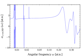
Figure 1: . The scalar polarisability of $\hbox{\rm HD}^{+}$ in the level $(v=1,\,L=1)$, computed using variational wave functions. Atomic units are used.

V.3.1 $\hbox{\rm H}_{2}^{+}$

For $\hbox{\rm H}_{2}^{+}$, we can compare our values of the scalar polarisability with the calculation by Pilon, who has communicated the values at six different frequencies Plion Pirvate comm . The values agree, with deviations of at most $2\times 10^{-6}$ atomic units in the range $\omega\leq 0.08$.

We show in Fig. 2 the frequency-dependent part of the polarisability of one level of $\hbox{\rm H}_{2}^{+}$, $\alpha_{s,var,{\rm H}_{2}^{+}}((1,\,1),\,\omega)-\alpha_{s,{\rm var,H}_{2}^{+}}((1,\,1),\,0)$, at low frequencies. For the computation of the BBR shift at 300 K, frequencies up to approximately $\omega=0.013$ atomic units are relevant. In this range the polarisability is quite close to quadratic in $\omega$. With increasing vibrational quantum numbers $v$, the deviations from quadratic are more pronounced.

The dynamic electronic BBR shift corrections $\Delta E_{dyn,elec}$ computed from the variational data (with an integration analogous to Eq. (27)) are shown in Table 8. We see that the correction is small in relative terms, $1\times 10^{-4}$ for $v=0$, increasing to $4\times 10^{-4}$ for $v=3$. It is very weakly dependent on $L$. Nevertheless, these results show that the dynamic contribution should not be omitted even within the non-relativistic approximation. When it is included, the overall inaccuracy is limited by the non-relativistic approximation to approximately $1\times 10^{-4}$ fractionally. For $v<6,\,L<6$ the total BBR shift is smaller than 0.1 Hz. Therefore, the absolute error is less than 0.01 mHz.

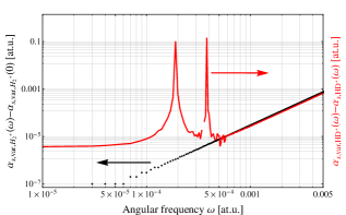
Figure 2: . Black (dotted line): the frequency-dependent contribution of the scalar polarisability of $\hbox{\rm H}_{2}^{+}$ in the level $(v=1,\,L=1)$, computed using variational wave functions. Red (gray, full line): difference between the scalar polarisability of $\hbox{\rm HD}^{+}$, also in the level $(v=1,\,L=1)$, computed variationally and approximately. The difference is noticeable close to the two rotational transition frequencies $(v=1,\,L=1)\rightarrow$$(v=1,\,L=0)$ and $(v=1,\,L=1)\rightarrow$$(v=1,\,L=2)$. A gap occurs in the red curve at $\omega=3.5\times 10^{-4}$ atomic units because the difference is negative.

V.3.2 $\hbox{\rm HD}^{+}$

For $\hbox{\rm HD}^{+}$, a comparison of the variational dynamic polarisability $\alpha_{s,var,{\rm HD}^{+}}(\omega)$ with the approximation $\alpha_{s,{\rm HD^{+}}}(\omega)=\alpha_{s}(\omega=0)+\delta\alpha_{s,dyn,rv}(\omega)$ is depicted in Fig. 2, which shows their difference. In evaluating the approximation, we have used both the transition dipoles of Tian et al. Tian et al and their non-relativistic energies, since also the variational polarisability was computed in non-relativistic approximation. The agreement is very good, except for small deviations near the transition frequencies (whose nominal contribution to the BBR shift is only of order $1.5\times 10^{-3}$ mHz), and a frequency-dependent contribution from the excited electronic states, which is again closely quadratic in frequency.

$\begin{array}[]{|c|c|c|c|c|}\hline\cr v&L&\omega_{min}(v,\,L)&\text{fit}&\text{$\Delta E_{dyn,elec}((v,\,L),\,T)$}\\ &&&&[{\rm mHz}]\\ \hline\cr\hline\cr 0&0&0.0015&16.10\,\omega^{3}+14.54\,\omega^{2}&-0.0021\\ 0&1&0.0015&16.24\,\omega^{3}+14.62\,\omega^{2}&-0.0021\\ 0&3&0.002&16.94\,\omega^{3}+15.01\,\omega^{2}&-0.0022\\ 0&4&0.003&17.58\,\omega^{3}+15.32\,\omega^{2}&-0.0022\\ 1&1&0.0015&48.34\,\omega^{3}+24.76\,\omega^{2}&-0.0036\\ 1&5&0.019&63.87\,\omega^{3}+25.86\,\omega^{2}&-0.0038\\ 2&4&0.02&148.1\,\omega^{3}+42.73\,\omega^{2}&-0.0063\\ 2&5&0.019&166.0\,\omega^{3}+42.92\,\omega^{2}&-0.0064\\ 3&2&0.04&395.8\,\omega^{3}+62.68\,\omega^{2}&-0.0094\\ \hline\cr\end{array}$

Table 11: Fourth column: polynomial approximation to $\alpha_{s,dyn,elec}(\omega)$, the frequency-dependent part of the contribution to the polarisability $\alpha_{s}$ of $\hbox{\rm HD}^{+}$ stemming from the excited electronic states. Fifth column: corresponding contribution to the BBR shift at 300 K. The angular frequencies $\omega$ and $\omega_{min}$ are in atomic units.

We have fitted a simple quadratic plus cubic polynomial to the difference $\alpha_{s,var}(\omega)-\alpha_{s,{\rm HD^{+}}}(\omega)$ between variational and approximate frequency-dependent polarisability, over the frequency range $\omega_{min}(v,\,L)$ to 0.05 at. u. Here, $\omega_{min}(v,\,L)$ is chosen appropriately so as to allow an accurate fit. These fits represent an approximation to $\delta\alpha_{s,dyn,elec}((v,\,L),\,\omega)$ for frequencies from 0 to 0.05 at. u. The fits are shown in Tab. 11. The contribution of the cubic term is seen to be small compared to the quadratic one for the range of frequencies relevant for the BBR shift at 300 K. Tab. 11 gives the corresponding contributions to the BBR shift, to be added to the other two contributions given in Tab. 10. The error in the values of $\Delta E_{dyn,elec}$ due to this fit treatment is on the order of 0.001 mHz. We see that this BBR shift contribution again varies weakly with $L$, but significantly with $v$ and that for levels with $v=3$ it reaches $1\times 10^{-5}$ Hz. Therefore, it needs to be taken into account even within the non-relativistic approximation, if no loss of accuracy is desired. When this is done, the total error of the BBR shift due to the non-relativistic approximation is expected to be $1\times 10^{-4}$ fractionally, or less than $0.03\,$mHz for the low-lying levels of $\hbox{\rm HD}^{+}$, $v<6$.

VI Conclusion

We have computed the non-adiabatic static polarisabilities of the molecular hydrogen ions $\hbox{\rm HD}^{+}$, $\hbox{\rm H}_{2}^{+}$, and $\hbox{\rm D}_{2}^{+}$, extending significantly previous results, mostly limited to rovibrational levels with rotational angular momentum $L=0,\,1$. For a number of rovibrational levels, we have also computed the frequency-dependent non-adiabatic polarisability.

The dependence of the polarisabilities on the hyperfine state has been derived and discussed in detail. We have pointed out the special case of the pure states, for which a simple analytical result has been derived. This result is actually a very good approximation for all hyperfine states of $\hbox{\rm H}_{2}^{+}$. The hyperfine-state-dependence is of crucial importance if a detailed understanding of the systematic shifts of transition frequencies is to be performed.

We have also computed the shifts induced by the black-body radiation field, and their temperature derivatives.

Emphasis has been given here to achieve high numerical accuracy. The effective relative inaccuracy of our computed values is about $1\times 10^{-4}$ due to the neglect of relativistic corrections. For for $\hbox{\rm H}_{2}^{+}$ and $\hbox{\rm D}_{2}^{+}$ this translates in an absolute inaccuracy of 0.001 at. u. for all levels with $v<6,\,L<5$. For $\hbox{\rm HD}^{+}$ in $L=0,\,1$ levels the inaccuracy is less than 0.1 at. u., and in $L\geq 2$, it is less than 0.003 at. u.. An inaccuracy of 0.1 atomic unit is sufficiently low to allow evaluating the Stark shift with a theoretical error corresponding to the $10^{-18}$ fractional frequency level, given the typical electric field values in ion traps.

In order to obtain accurate values of the black-body radiation shift, we have used accurate values of the transition dipoles and we have analyzed the importance of the contributions from excited electronic states. We estimate the inaccuracy of the shifts to be less than 0.03 mHz for levels with $v<6,\,L<6$, at 300 K, for both $\hbox{\rm HD}^{+}$ and $\hbox{\rm H}_{2}^{+}$. This corresponds to theoretical fractional frequency errors on the order of $1\times 10^{-18}$.

Using the present results it becomes possible to identify theoretically transitions having low sensitivity to external fields Bakalov and Schiller 2013 ; Schiller Bakalov Korobov PRL 2014 . This represents an important aspect in the future spectroscopy of the simplest stable molecules.

We thank Dr. Olivares Pilón for communicating unpublished results.

References

- (1) B. Grémaud, D. Delande, and N. Billy, J. Phys. B 31, 383 (1998).
- (2) see V.I. Korobov, L. Hilico, and J.-Ph. Karr, “-order QED corrections in the hydrogen molecular ions and antiprotonic helium”, Phys. Rev. Lett. 112, 103003 (2014) and references therein.
- (3) J.C.J. Koelemeij, B. Roth, A. Wicht, I. Ernsting, and S. Schiller, Phys. Rev. Lett. 98, 173002 (2007).
- (4) U. Fröhlich, B. Roth, P. Antonini, C. Lämmerzahl, A. Wicht, S. Schiller, in Seminar on Astrophysics, Clocks and Fundamental Constants, E. Peik, S. Karshenboim, eds., Lecture Notes in Physics, Springer, 648, 297 (2004)
- (5) S. Schiller and V.I. Korobov, Phys. Rev. A 71, 032505 (2005).
- (6) K. B. Jefferts, Phys. Rev. Lett. 23, 1476 1969.
- (7) W.H. Wing, G.A. Ruff, W.E. Lamb, Jr., and J. J. Spezeski, “Observation of the Infrared Spectrum of the Hydrogen Molecular Ion HD+”, Phys. Rev. Lett. 36, 1488–1491 (1976); doi/10.1103/PhysRevLett.36.1488;
- (8) A. Carrington et al., Mol. Phys. 72, 735 (1991); doi: 10.1080/00268979100100531
- (9) S. Schiller, C. Lämmerzahl, Phys. Rev. A 68, 053406 (2003).
- (10) P. Blythe, B. Roth, U. Fröhlich, H. Wenz, S. Schiller, “Production of cold trapped molecular hydrogen ions”, Phys. Rev. Lett. 95, 183002 (2005); doi:10.1103/PhysRevLett.95.183002
- (11) U. Bressel, A. Borodin, J. Shen, M. Hansen, I. Ernsting, and S. Schiller, “Manipulation of Individual Hyperfine States in Cold Trapped Molecular Ions and Application to Frequency Metrology”, Phys. Rev. Lett. 108, 183003 (2012)
- (12) J. Shen, A. Borodin, M. Hansen, und S. Schiller, “Observation of a rotational transition of trapped and sympathetically cooled molecular ions“, Phys. Rev. A 85, 032519 (2012).
- (13) D. Bakalov, V.I. Korobov and S. Schiller, “Precision spectroscopy of the molecular ion : control of Zeeman shifts”, Phys. Rev. A 82, 055401 (2010).
- (14) D. Bakalov, V.I. Korobov and S. Schiller, “Magnetic field effects in the transitions of the molecular ion and precision spectroscopy”, J. Phys. B: At. Mol. Opt. Phys. 44, 025003 (2011); Corrigendum: J. Phys. B: At. Mol. Opt. Phys. 45, 049501 (2012).
- (15) J.-P. Karr, V.I. Korobov, L. Hilico, “Vibrational spectroscopy of : Precise evaluation of the Zeeman effect”, Phys. Rev. A 77, 062507 (2008)
- (16) D. Bakalov and S. Schiller, “The electric quadrupole moment of molecular hydrogen ions and their potential for a molecular ion clock”, Appl. Phys. B 114, 213-230 (2014); DOI 10.1007/s00340-013-5703-z
- (17) S. Schiller, D. Bakalov, V. I. Korobov, arXiv:1402.1789; Phys. Rev. Lett. (accepted).
- (18) J.C.J. Koelemeij, “Infrared dynamic polarisability of rovibrational states”, Phys. Chem. Chem. Phys. 13, 18844 (2011).
- (19) D. M. Bishop and B. Lam, “An analysis of the interaction between a distant point charge and ”, Mol. Phys. 65, 679-688 (1988)
- (20) L. Hilico, N. Billy, B. Grémaud, D. Delande, “Polarisabilities, light shifts and two-photon transition probabilities between states of the and molecular ions”, J. Phys. B. 34, 491 (2001)
- (21) R.E. Moss, and L. Valenzano, “The dipole polarisability of the hydrogen molecular cation and other isotopomers”, Molec. Phys. 100, 1527 (2002).
- (22) Z.C. Yan, Y.J. Zhang, and Y. Li, Phys. Rev. A 67, 062504 (2003)
- (23) J.-Ph. Karr, S. Kilic, and L. Hilico, “Energy levels and two-photon transition probabilities in the ion”, J. Phys. B: At. Mol. Opt. Phys. 38, 853 (2005).
- (24) A. K. Bhatia, R. J. Drachman, Phys. Rev. A 61, 032503 (2000)
- (25) V.I. Korobov, Phys. Rev. A 61, 064503 (2000)
- (26) D. Bakalov and S. Schiller, “Static Stark effect in the molecular ion ”, Hyperfine interact. 210, 25 (2012)
- (27) H. Olivares Pilón and D. Baye, “Static and dynamic polarisabilities of the non-relativistic hydrogen molecular ion”, J. Phys. B: At. Mol. Opt. Phys. 45, 235101 (2012); http://iopscience.iop.org/0953-4075/45/23/235101
- (28) This result was first presented at the 2nd COST IOTA Workshop on Cold Molecular Ions, Arosa (Switzerland), September 2013.
- (29) V.I. Korobov, L. Hilico, and J.-Ph. Karr, Phys. Rev. A 74, 040502(R) (2006).
- (30) J. Ph. Karr, F. Bielsa, A. Douillet, J. Pedregosa, V. I. Korobov, and L. Hilico, Phys. Rev. A 77, 063410 (2008).
- (31) D. Bakalov, V.I. Korobov, and S. Schiller, “High-precision calculation of the hyperfine structure of the ion”, Phys. Rev. Lett. 97, 243001 (2006).
- (32) A Messiah, Quantum Mechanics, (vol. II, Appendix C, § 15), North Holland, Amsterdam, 1961.
- (33) D.A. Varshalovich, A.N. Moskalev, and V.K. Khersonskii, Quantum Theory of Angular Momentum, (World Scientific, Singapore, 1988).
- (34) I. Roeggen, “The theory of the Stark effect in multiplet states of diatomic polar molecules”, J. Phys. B: At. Mol. Opt. Phys. 4, 168 (1971); http://iopscience.iop.org/0022-3700/4/2/004
- (35) Q.-L. Tian, L.-Y. Tang, Z.-X. Zhong, Z.-C. Yan, T.-Y. Shi, “Oscillator strengths between low-lying ro-vibrational states of hydrogen molecular ions“. J. of Chem. Phys. 137, 024311 (2012). doi:10.1063/1.4733988.
- (36) V.I. Korobov, “Leading-order relativistic corrections to the ro-vibrational spectrum of and molecular ions”, Phys. Rev. A 74, 052506 (2006).
- (37) V.I. Korobov and Zhen-Xiang Zhong, “Bethe Logarithm for the and molecular ions, Phys. Rev. A 86, 044501 (2012).
- (38) R. E. Moss, “Calculations for vibration-rotation levels of HD+, in particular for high N“. Molecular Physics 78, 371–405. doi:10.1080/00268979300100291.
- (39) T.N. Rescigno, and V. McKoy, Phys. Rev. A 12, 522 (1975).
- (40) V.I. Korobov, “Dynamic polarisability properties of the weakly bound ddμ and dtμ molecular ions”, J. Phys. B 37, 2331–2341 (2004), DOI: 10.1088/0953-4075/37/11/010
- (41) Online at: (**** to be filled by editor ****). Each line of the data files has the format: (in atomic units), (in atomic units), (in atomic units). Note that for and there is a difference of 0.0001 at. u. between the value of the data file and the value in 1. This arises from the numerical procedure used, which was optimized towards good accuracy for high up to the continuum threshold. Note that the values of in the files should be multiplied with for actual computations.
- (42) H.O. Pilón, priv. comm. (2013)