Spatial Nonlocality of the Small-Scale Solar Dynamo

Abstract

We explore the nature of the small-scale solar dynamo by tracking magnetic features. We investigate two previously-explored categories of the small-scale solar dynamo: shallow and deep. Recent modeling work on the shallow dynamo has produced a number of scenarios for how a strong network concentration can influence the formation and polarity of nearby small-scale magnetic features. These scenarios have measurable signatures, which we test for here using magnetograms from the Narrowband Filter Imager (NFI) on Hinode. We find no statistical tendency for newly-formed magnetic features to cluster around or away from network concentrations, nor do we find any statistical relationship between their polarities. We conclude that there is no shallow or “surface” dynamo on the spatial scales observable by Hinode/NFI. In light of these results, we offer a scenario in which the sub-surface field in a deep solar dynamo is stretched and distorted via turbulence, allowing the field to emerge at random locations on the photosphere.

1. Introduction

The Sun is covered in a pattern of “salt and pepper” small magnetic features that dominate the star’s photospheric magnetic energy budget (Babcock, 1953). The generation of large-scale magnetic fields in the interior and on the surface of the Sun is understood to be a consequence of rotational motion, large-scale convection, the transport of magnetic fields to the poles, and the storage of intensely strong magnetic fields at the base of the convection zone, though many important questions remain unanswered (Charbonneau, 2010). The origin of magnetic fields on much smaller spatial scales, scales of order the supergranular ($\sim$15–30 Mm) size, granular ($\sim$1 Mm) size, or smaller, is not as well understood. These small-scale magnetic fields are important for the overall magnetic flux and energy budgets of the Sun, and are important in structuring and heating the chromosphere and corona.

On one hand, it is possible that the fields seen on these small scales are produced as a consequence of the global, large scale (mean field) dynamo. In this scenario, the convective buffeting of the fields at the surface and in the interior shreds them to smaller and smaller scales, down to (and likely further than) the resolution limit of currently available telescopes. Evidence of this model is given by simulations of magnetoconvection that show invariance across a wide range of scales (Stein & Nordlund, 2006) and by observations that the probability distribution of magnetic flux concentrations shows a smooth $-1.8$ power-law distribution over nearly 6 orders of magnitude in magnetic flux (Parnell et al., 2009).

On the other hand, it is possible that a shallow near-surface “small-scale” dynamo is present, and that even without the global dynamo, magnetic fields would continue to be generated and amplified by the small-scale flows. Recent observational evidence, primarily from Hinode, lends some credence to this scenario. Examples include the patterns of horizontal magnetic fields in the photosphere (Lites et al., 2008) and the lack of a change in the numbers of weak magnetic features in the quiet sun when measured as a function of the solar cycle phase (Buehler et al., 2013).

Several groups have produced impressively realistic-looking simulations that amplify a small seed field into something that looks and behaves like the observed magnetic network (e.g., Cattaneo, 1999; Vögler & Schüssler, 2007). However, as Stenflo (2012) recently pointed out, evidence for small-scale dynamo activity in these simulations is not necessarily evidence for small-scale dynamo activity on the Sun, as the results typically depend strongly on the initial conditions or the approximations used. Due to unavoidable computational limitations, current state-of-the-art simulations are forced to operate in a physical regime in which the Reynolds number $Re$, magnetic Reynolds number $Re_{M}$, and magnetic Prandtl number $Pm$ are (sometimes vastly) dissimilar to the actual properties of the Sun. Thus while the simulations are useful for understanding the size scales, expected magnetic phenomenology, and interaction of any generated fields with larger-scale fields, progress in understanding the existence of and role played by a small-scale dynamo is, for now, best made by observational analysis.

There is a third alternative to the problem of the small-scale flux: a small-scale dynamo in which the dual processes of stretching of the seed field and the addition of the new field to the photosphere are not in close proximity to each other-the new field may be observed at an essentially random location with respect to the original field. Such a dynamo could be driven by turbulent convection throughout the full depth of the convection zone without the proximity properties one would expect of a shallow surface dynamo. This possibility is supported by simulations that show cool downdrafts extending through the turbulence of the outer solar layers to the base of the convection zone (e.g., Stein et al., 2003). If this possibility is correct the cross-scale equilibrium (Schrijver et al., 1997) could drive energy flow in either direction: large to small scales, or vice versa (e.g., Vögler & Schüssler, 2007). We refer to this possibility as a “spatially nonlocal small-scale dynamo”, where “spatially” is meant to distinguish (non-)locality in physical space from (non-)locality in wavenumber space.

Dynamos are a mechanism for creating magnetic fields, but in order for a dynamo to operate indefinitely, there must be a way to stem the continued growth of the field. Otherwise, the photosphere would quickly become choked with magnetic fields and convection suppressed, which is obviously not the case as can be seen in any photospheric line-of-sight magnetogram. Very generally, this stemming of the growth of the field may take two forms: in the first, existing magnetic field is removed in cancellation / flux annihilation events; in the second, the production of new flux is suppressed. While the cancellation events have been studied for decades, the suppression of continued generation of magnetic flux (apart from sunspots) is less extensively studied. Two relatively recent examples include the work of Morinaga et al. (2008), in which convection (and thus presumably dynamo action) was reduced in the presence of small-scale magnetic features such as G-band bright points, and the work of Hagenaar et al. (2008), in which the emergence rate of large-scale ephemeral regions was found to be reduced in areas of strong unipolar magnetic fields (including but not limited to coronal holes).

1.1. Outline

In this paper, we bridge the gap between the works of Morinaga et al. (2008) and Hagenaar et al. (2008) and investigate the spatial relationship between existing strong-field regions and the detection of new magnetic features, which we take as a proxy for dynamo action, at intermediate spatial scales. We focus on the areas around supergranular network flux concentrations, and analyze whether the rate of feature birth at a range of distances from the network concentration is significantly larger or smaller than would be expected from a random distribution of events.

In addition to occupying an interesting intermediate spatial scale, supergranular network concentrations are an ideal observational target: their field strength and flux is high enough that they might reasonably have a positive or negative effect on any spatially local small-scale dynamo activity, their occurrence is common enough that several will exist in a reasonably-sized dataset, and they are sufficiently long-lived such that the surrounding plasma can be affected by their presence. Our criteria for identifying network concentrations is given in Section 2.2. Our goal was to identify whether the rate of detection of new magnetic features has some dependence on the distance from the network concentration.

In this work we use the number of features as a proxy for the rate of flux production. This enables us to explore four mechanisms by which the number of features at short distances from a network concentration could be altered. In the case of suppression, for example, fewer features should be found near the borders of the concentration, while more features per unit area should be found further away.

Three forms of feature evolution are illustrated in Figure 1. Shredding (Figure 1a) involves field lines that are bodily moved away from the network concentration. This results in a decrease of the concentration’s flux as the field lines move away, and the features have the same polarity as the network concentration. Stretching (Figure 1b) involves field lines from below the surface that are stretched and brought to the surface. Such distorted field components would then appear on the Sun as newly-formed small-scale features. Here the flux of the concentration remains the same, the total unsigned flux in the region increases, and the new, nearby features have a mixed polarity. This is the chief mechanism we search for as evidence of spatially local small-scale dynamo action. Canceling (Figure 1c) involves field lines of opposite polarity to the network concentration that are brought towards it and cancel with it. In this case the flux of the network concentration decreases and the unsigned flux of the region also decreases.

Figure 1.— Three mechanisms which could result in an increase in detected features near a network concentration. a) As the network concentration is shredded, flux is removed from the edge of the concentration, possibly (but not necessarily) in a way that eludes detection, as shown. b) Network concentration field lines below the surface are stretched and brought to the surface. c) Opposite polarity flux impinges on the network concentration and cancels.

Section 2 describes the dataset and feature tracking method, the means for identifying network concentrations, and the method used to measure suppressions and enhancements of features around the network concentrations. Section 3 presents our results. We find no signature of systematic enhancement or suppression of magnetic feature production in the vicinity of the network concentrations. Instead, we find that most measured suppressions and enhancements can be attributed to network concentration evolution, as shown in Section 4. Further, we find that there is no statistical tendency for these magnetic features to cluster around network concentrations. Section 5 concludes with a discussion on the implications of these null measurements and the importance of small-scale fields to network concentration evolution.

2. Methodology

2.1. Data Processing

We use line-of-sight magnetograms from the Hinode/NFI instrument (Kosugi et al., 2007; Tsuneta et al., 2008). The dataset and its preparation was described in detail by Lamb et al. (2010). Briefly, the data consist of a 5.25 h long sequence of 420 $277"\times 96"$ (0.16” pixels) Na D 5896 Å magnetograms with a cadence of 45 s, beginning at 2007-09-19 12:44:44 UT and ending at 17:58:59 UT. The observed region was just south of disk center, in a region of quiet sun, and Hinode tracked the region as it rotated across the disk. The magnetograms were converted from raw Stokes I & V images, which were then de-spiked to remove cosmic rays, de-rotated to a common reference frame, and temporally averaged using a Gaussian weighting. The temporal averaging function had a FWHM of 2 frames (1.5 minutes) and preserved the 45-second cadence of the original data. Finally, the magnetograms were spatially smoothed by convolving them with a $3\times 3$ 2-pixel FWHM Gaussian kernel $k=\frac{1}{16}\times\left[\begin{array}[]{ccc}1&2&1\\ 2&4&2\\ 1&2&1\end{array}\right]$ .

2.2. Feature and Network Concentration Tracking

For feature tracking, we used the SWAMIS magnetic feature tracking code (DeForest et al., 2007) with following parameters: thresholds of 18 & 24 G, $x-y-t$ diagonals disallowed in the detection hysteresis, a per-frame minimum size of 4 pixels, a minimum lifetime of 4 frames, and a minimum total of 8 pixels over each feature’s lifetime. We used both the “downhill” and the “clumping” methods of feature identification. The “downhill” method groups pixels into features by finding local maxima (for positive pixels) and working downhill until a local minimum is found (and oppositely for negative pixels), and is better for finding the small-scale structure of the magnetic fields. The “clumping” method groups all adjacent same-signed pixels into the same feature, and is better for finding the large-scale structure of the magnetic fields. For example, a large supergranular network concentration will be counted as only one feature by the “clumping” method, but as many features by the “downhill” method (DeForest et al., 2007; Parnell et al., 2009). The downhill method identified 112217 features, while the clumping method found 53910 features throughout the 5.25-hour time span of the dataset.

Network concentrations were identified using the clumped feature tracking data. A feature was designated a network concentration if it was present for the entire length of the dataset and had a peak flux density $>500\textrm{ Mx}\textrm{ cm}^{-2}$ in the first frame. We ignored network concentrations measured within 100 pixels of the edge of the field of view, so as to remove the complication of edge effects. We identified seven network concentrations using this method; they are shown on a single frame in Figure 2. As expected, the identified network concentrations were separated by distances of 15–30 Mm, which is approximately the range of supergranule diameters (Meunier et al., 2007).

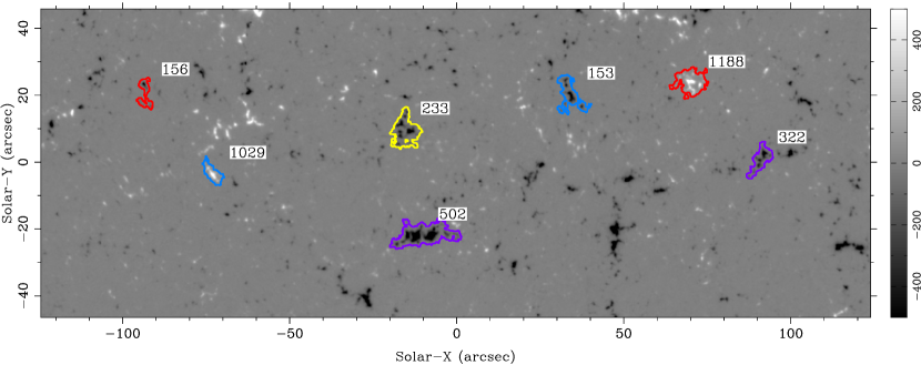
Figure 2.— The seven network concentrations identified using the SWAMIS tracking code described in the text. The background magnetogram is the initial frame in the dataset (2007-09-19 at 12:44:44), and the colored outlines show the extent of the network concentrations in that frame. The numbers next to each concentration are the feature ID numbers SWAMIS assigned while using the “clumping” method, and are used throughout the paper.

2.3. Removing “Wander”

Hinode’s pointing “wander”, which translates the frames by many pixels on timescales of tens of minutes, posed a problem at the spatial scales used in the present study. The wander is not recorded in the reported scientific coordinates (arcseconds from disk center) in the Hinode FITS files, so other means of removing it were required.

We determined a pointing offset between each pair of frames by taking the median horizontal and vertical displacement across all features common to those two frames, attributing the net displacement entirely to residual solar rotation and pointing drift (Figure 3a). The horizontal drift varied between $-0.63"$ and $0.75"$, but we found a more steady positive vertical drift. A linear least-squares fit to the vertical drift, requiring that the line intersect the origin, reveals a $0.98"\textrm{ hour}^{-1}$ drift northward (Figure 3b).

Figure 3.— Hinode’s pointing “wander”, derived from the median horizontal and vertical frame-to-frame change in the position of features. a) Total wander as a function of time. The beginning of the datasets is at (0,0). For clarity, only every other point has been plotted, and note the reversed abscissa and ordinate. The large crosses show the wander on 1-hour intervals. b) Vertical component of wander plotted with time. The dashed line is the first-order least-squares fit that includes the constraint that it intersects the origin. Its slope is $0.98"\textrm{ hour}^{-1}$.

The drift was derived from the clumping tracking method; the drift derived from downhill tracking has the same overall shape but is systematically smaller by about 5%. We attribute this to greater “noise” in the clumping signal, because the flux-weighted center-of-gravity of the larger clumped features is more affected by merging and fragmenting of flux. Nevertheless, we use the drift derived from the clumping dataset, since that method was used for network concentration identification (Section 2.2).

3. Statistical Analysis & Results

Our objective was to identify whether there is a tendency for new features to cluster or avoid regions near to or away from network concentrations. This required a statistical evaluation of the location and polarity of new features compared with that of the concentration. Computer code used to conduct the statistical analysis and produce the figures can be obtained by contacting the lead author.

3.1. The Position of New Features Around Network Concentrations

While the clumping method allows for easier identification of the network concentrations, more precise spatial locations are obtained with the downhill method since the same “clumped” feature is broken into several smaller features. Thus, for every frame, we found those downhill features that were at the location of the network concentration identified in the clumped data. Throughout the dataset, each network concentration changed in size and shape (this is explored further in Section 4), and so together these downhill features describe the network concentration’s maximum spatial extent (green outline in Figure 4), adjusted to accommodate for the Hinode pointing wander.

We identified all small-scale features within 100 pixels (11.6 Mm) of the network concentrations’ initial flux-weighted center-of-gravity (the cyan dot in Figure 4). We excluded those features that were present at the beginning of the dataset, along with those that were created via the “Fragmentation” or “Error” categories (see Lamb et al., 2008, 2010, for descriptions of these categories of feature creation). The locations of the selected features are indicated by the blue dots in Figure 4, superimposed on top of a section of the first frame in the dataset. This shows every new feature location regardless of the time at which it was created, so there is little-to-no temporal relationship between the underlying magnetogram in the figure and the blue dots. The blue dot locations also accommodate for wander.

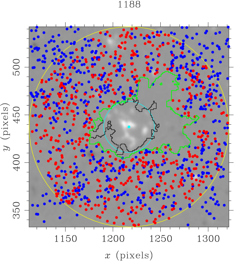
Figure 4.— A selected $212\times 212$ pixel area on the first frame (2007-09-19 at 12:44:44UT, chosen purely for convenience) in our dataset showing the network concentration numbered 1188 in Figure 2. Background: magnetogram from the selected area in this first frame. Cyan dot and circle: center-of-flux and initial circularized area of the concentration. Black outline: initial area of the concentration. Green outline: maximum spatial extent of the concentration. Blue dots: locations of new features (not born by Fragmentation or Error) during the entire sequence. Red dots: random locations, the generation of which is described in Section 3.2. Note that the blue dots indicate the locations of new features throughout the entire dataset and do not contain information on the timing of the feature’s appearance.

3.2. Monte Carlo Simulations

In order to test whether there is a statistical tendency for the number of new features to be enhanced or suppressed in proximity to a network concentration, we measured their birth locations against that of a generated set of pseudo-random points. For each network concentration, we assigned points using a Monte Carlo procedure with $10^{4}$ iterations within the 200-pixel diameter circle (the yellow circle in Figure 4). These are hereafter referred to as random points, are shown as red dots in Figure 4, and were assigned according to the following criteria:

1. The number of random points (red dots in Figure 4) was equal to the number of detected features (blue dots) inside the circle;

2. Random points were not placed within the maximum spatial extent of the network concentration (outlined in green in Figure 4).

The number of points in a 5-pixel-wide annulus, centered on the center-of-gravity of the network concentration, and plotted against the radius of the center of the annulus, is shown in Figure 5. The blue points are the numbers of blue dots (new features) in Figure 4 within the annulus, and the vertical dotted line is the radius of the circularized initial area of the concentration (the cyan circle in Figure 4). The red points are the mean of the $10^{4}$ iterations of the random placement, and the error bars correspond to the 95th percentile around the mean.

Statistically, this graph can be interpreted as follows: If the placement of the new features lies within the uncertainty bounds of the random distribution, then they too are most likely randomly distributed, i.e., there is no statistical bias towards new features forming at that particular distance from the network concentration.

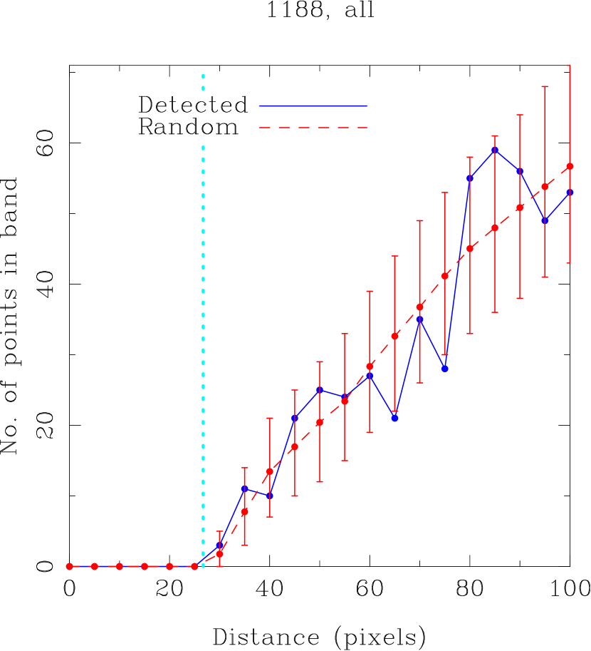
Figure 5.— For network concentration 1188 (the same as that shown in Figure 4), the number of points in a 5-pixel wide annulus centered on the cyan dot. The vertical cyan dotted line corresponds to the radius of the cyan circle in Figure 4. The blue points correspond to the blue dots (detected features) in Figure 4. The red points are the mean of $10^{4}$ iterations of the random placement, the error bars correspond to the 95th percentile around the mean.

Plots similar to Figures 4 and 5, but for the remaining six network concentrations, are shown in Figures 5 and 5. The three plots correspond to three different annular widths, of 5, 10 and 15 pixels. For the 15-pixel wide annuli, the radius of the region of interest was expanded to 105 pixels.

=0pt

Locations of new features around the remaining six network concentrations, with plots for three different annular widths of 5, 10 and 15 pixels.

=0pt

=250pt

Continuation of Figure 5.

=0pt

3.3. Quantitative Tests of Feature Number Enhancement and Suppression

As discussed in Section 1, removal of existing field and/or suppression of the dynamo mechanism is necessary in order to prevent the field from growing indefinitely. Suppression of some kind (including nonlinearity) is necessary to obtain a nonzero steady state for the field–which is impossible for a strictly linear dynamo mechanism. Spatially-local suppression would be manifest by an absence in the occurrence of new features in the proximity to a network concentration or, equivalently, an enhancement of new features far away. We can therefore identify the presence or absence of spatially-local suppression by comparing the appearance of new features with that of the random result.

For each network concentration, and for each 5-, 10-, or 15-pixel-wide annulus around that network concentration, we produced a histogram of the number of random points placed in each annulus by the $10^{4}$ Monte Carlo simulations. We denote the central value of the $j$th of $n$ bins of the histogram as $x_{j}$ and the histogram value to be $h(x_{j})$, such that $\sum_{j=1}^{n}h(x_{j})=10^{4}$. As a useful check, we observed the sample $h(x_{j})$ to have a distribution that is very close to Gaussian. We directly measured the mean $\mu$, standard deviation $\sigma$, and the scaling factor $A$ of the sample, and from those values derived (not fit) the analytic Gaussian profile of the sample

$$y(x_{j})=A\exp(-(x_{j}-\mu)^{2}/2\sigma^{2})$$ (1)

We then calculated the reduced $\chi^{2}$ statistic (Bevington & Robinson, 2003),

$$\chi_{\nu}^{2}=\frac{1}{\nu}\sum_{j=1}^{n}\frac{[h(x_{j})-y(x_{j})]^{2}}{h(x_{j})},$$ (2)

where $\nu=n-n_{c}$ is the number of degrees of freedom, with $n_{c}=3\,:\,(A,\sigma,\mu)$ being the number of constraints. The range of the histogram $x_{j}$’s was truncated so that $h(x_{j})>10$ in order to ameliorate uncertainties in the normality assumption for small numbers. $\chi_{\nu}^{2}$ provides a measure of the goodness of fit of the analytical profile $y(x_{j})$ to the Monte Carlo sample data $h(x_{j})$, and here tends to be between 1 and 2, with most of the contribution coming from the flanks of the distribution. $\chi_{\nu}^{2}$ does not contain any information about the number of detected magnetic features, only how well the distribution of the number of random points in an annulus approximates a Gaussian.

Using this estimate of the goodness of fit as a guide, for each network concentration and for each annulus, we determined the fraction $P$ of the simulations for which the measured number of new features $N$ in the annulus exceeded the number of random points. This was done for enhancements above the mean and suppressions below the mean separately, so that alternating high and low values (indicating too-small sampling bins) would average out when interpolated to larger bins. By definition,

$$P= 1-\frac{\sum_{x_{j}\geq N}y(x_{j})}{\sum_{x_{j}\geq\mu}y(x_{j})}, N\geq\mu$$

$$P= -1+\frac{\sum_{x_{j}<N}y(x_{j})}{\sum_{x_{j}<\mu}y(x_{j})}, N<\mu$$ (3)

The interpretation of $P$ is as follows:

• A value close to 0 indicates that the number of new features does not differ significantly from the number expected from a random distribution;

• A value close to $\pm 1$ indicates that the number of new features greatly exceeds or is greatly exceeded by that expected from a random distribution.

To account for the goodness of fit of $y(x_{j})$ to the sample data, particularly at small distances where the number of points in an annulus is small, we scale $P$ at each radius by the corresponding value of $\chi_{\nu}^{2}$, $Px=\frac{P}{\chi_{\nu}^{2}}$. Then, we added the values of $Px$ for each of the different annuli widths to produce $Px_{tot}$. In this way, we try to account for the fact that it is difficult to say what is the “correct” single annulus width to choose. The 5-pixel-wide annulus is probably too thin and results in large positive excursions adjacent to large negative excursions in Figures 5 and 5. By summing each $Px$ to produce $Px_{tot}$, we require that any excursions must be more-or-less independent of the resolution of our measurement, which is the annulus width.

For the annulus widths of 10 and 15 pixels we accumulate the values of $P$ into the corresponding 5-pixel bins. Since the values of $Px$ are not systematically smaller or larger among the three different annulus widths, a given value in the 15-pixel case transfers directly to the three corresponding 5-pixel bins, and to the two corresponding bins in the 10-pixel case. The individual values of $Px$ in each bin were added algebraically to produce the total $Px_{tot}$ in each 5-pixel wide bin (Figure 6).

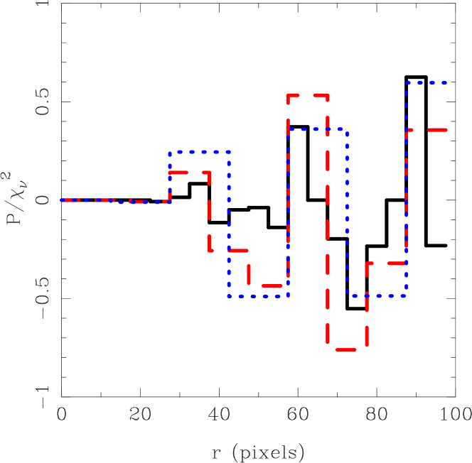
Figure 6.— For network concentration 153, the quantity $\frac{P}{\chi_{\nu}^{2}}$ as a function of distance from the network concentration center, for annuli with widths 5 pixels (solid black line), 10 pixels (dashed red line), and 15 pixels (dotted blue line). As described in Section 3.3, a value close to 0 indicates that the number of detected features in that annulus does not differ significantly from the number exepcted from a random distribution, and a large positive (negative) values indicates that the number of features is greater (less) than the expected values.

As shown in Figure 6, $P$ is generally closer to 0 than 1 ($|\frac{P}{\chi_{\nu}^{2}}|\leq 0.6P$) indicating a statistical preference towards a random distribution, i.e., no tendency for new features to form away from the network concentration. We conclude that there is no detectable anomalous spatially-local suppression taking place.

3.4. Polarity

Section 3.3 demonstrates that the new features identified in the present study were not subject to suppression. We now explore the mechanism responsible for their enhancement. In Section 1.1, we described three enhancement possibilities, illustrated in Figure 1: shredding, stretching and canceling. Each has a unique measurable affect on the polarity of the new features near the network concentration, as shown in Table LABEL:tab:NC-mod-polarity-truth.

Table 1Effect of the flux modification of network concentrations and their surroundings, and what polarity of new features would be expected to be enhanced in the concentrations’ surroundings.

	All	Like	Opposite
Shredding	Y	Y	N
Stretching	Y	Y	Y
Canceling	Y	N	Y

We first only considered those features with the same sign as the network concentration (a possible signature of either shredding or of stretching), and determined their $Px_{tot}^{+}$. Then, we only considered those detected features with the opposite sign as the network concentration (a signature of canceling or stretching), and determined $Px_{tot}^{-}$.

$Px_{tot}(r)$ provides a measure, as a function of distance from the center of the network concentration, of the deviation of the number of features from the number of random points in an annulus. It takes into account the uncertainty in the expected number of points, differences in the number of detected features among the network concentrations, as well as differences that may arise by changing the bin size. Plots of $Px_{tot}(r)$, as well as $Px_{tot}^{+}(r)$ and $Px_{tot}^{-}(r)$ for each of the seven network concentrations are shown in Figure 7.

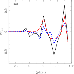
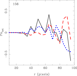
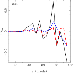
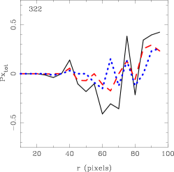
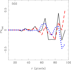
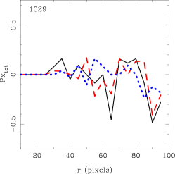
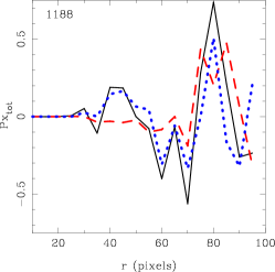
Figure 7.— Values of $Px_{tot}$ as a function of distance from the network concentration center, which indicates the enhancement (for large positive values) or suppression (for large negative values) or lack thereof (for values close to 0) of the number of new features around each network concentration. The three curves correspond to $Px_{tot}$ (solid black; all features), $Px_{tot}^{+}$ (dashed red; only features of the same polarity as the network concentration) and $Px_{tot}^{-}$ (dotted blue; only features of the opposite polarity as the network concentration).

Since $Px_{tot}$ is a continuous variable, it is useful to have some indicator of when its value is significantly different from 0. For annuli widths of 5 pixels, the RMS value of $Px\approx 0.25$. It is qualitatively larger for the larger annuli, though the sample size is small for large annuli. We sum $Px$ over three annulus sizes (5, 10, & 15 pixels), arriving at an overall threshold for $Px_{tot}$ of 0.75 ($\approx 2\sigma$). None of the Figure 7 network concentrations have a $Px_{tot}$ that exceeds $\pm 0.75$ at any radius.

We do note that for 3 of the 7 network concentrations studied, there is a peak in the number of features at distances of $\approx 75-90$ pixels. The peaks are not significant in the individual concentrations, nor across the ensemble. Further they are limited to 1–3 pixel bins in width, and do not have the shape expected from the mechanisms we discuss. We therefore reject all three possibilities for a spatially local small-scale dynamo described in Table LABEL:tab:NC-mod-polarity-truth.

4. Network Concentration Evolution

Our analysis allows us to quantify regions of interest for specific network concentrations. The results are averages over many things: azimuthal angle around the network concentration, annuli widths, and most importantly the 5.25 hour duration of the dataset. In order to fully understand the interplay between the concentration and the surroundings, we must also examine the evolution of the network concentrations themselves.

Many things can affect the evolution of a network concentration. An old supergranule may decay, and/or a new one may form, changing the locations of the downflow vertex. The downflow may move in response, or it may cease to exist entirely, and the flux in the network concentration may be dispersed to the lanes of the new supergranule.

The introduction of new flux into an existing flow pattern will also affect the network concentration. A strong bipolar region may form in the interior of the supergranule, driving flux to the vertex containing the existing concentration. Like-polarity flux will increase the strength of the network concentration, while opposite-polarity flux will cancel and weaken the concentration.

Figure 8 shows the flux magnitude evolution of each of the seven network concentrations across the dataset. Each curve has been convolved with a 10-frame boxcar kernel to smooth out short-term variations, and then normalized by its initial value. Several of the network concentrations lose large fractions of their flux over the 5.25 hours; three lose more than 50%. Table LABEL:tab:NC-Properties describes various evolution properties of the network concentrations and their surroundings. Note that edge effects due to the convolution cause some concentrations’ final fluxes to appear slightly different in Figure 8 than reported in Table LABEL:tab:NC-Properties.

Figure 8.— Evolution of network concentration flux. The lines shown here have been convolved with a 10-frame boxcar function to smooth out short term variations, and then normalized by their initial values.

Table 2Properties of selected network concentrations and their surroundings. The network concentrations’ flux ($\Phi$) and flux density ($\langle B\rangle$), and the surroundings’ flux imbalance ($\xi$) and unsigned flux density ($\langle|B|\rangle$), are all medians taken over the length of the dataset. The network concentrations’ change in flux $\frac{\Phi_{F}}{\Phi_{I}}$ uses the raw, unsmoothed data.

Network Concentration				Surroundings
ID	$\Phi(10^{18}\textrm{ Mx})$	$\langle B\rangle$ (G)	$\frac{\Phi_{F}}{\Phi_{I}}$(%)	$\xi$ (%)	$\langle\left|B\right|\rangle$ (G)	Evolution Summary
N/A	N/A	N/A	N/A	12.1	7.91	(Dataset taken as a whole)
153	16.7	-97.8	48	26.0	12.0	Nearby opp. polarity, but NC shredding
156	9.75	-93.4	174	28.3	11.5	much merg/frag to make a distinct NC
233	32.9	-127	84	17.5	9.58	much merg/frag to make a distinct NC
322	18.5	-110	59	47.9	8.49	steadily cleaving off field
502	90.2	-158	92	-39.0	8.85	very large NC, not much change
1029	10.1	+104	47	47.9	15.4	shredding trailing side, cancel leading side
1188	23.7	+103	45	-42.5	9.23	NC cancellation

Movies of the network concentration evolution suggest that the dynamics of the concentrations themselves are likely to dominate the surroundings, and other quantities listed in Table LABEL:tab:NC-Properties confirm this idea. For example, Concentration 1188 shows a 55% decrease in flux over 5.25 hours, and has an enhancement of detected features due to features of polarity opposite to itself. The flux imbalance of the surroundings is defined as the ratio of the net flux to the absolute flux (see Hagenaar et al., 2008, Eq. 1)

$$\xi\equiv S\times\frac{\Sigma\Phi_{i,j}}{\Sigma|\Phi_{i,j}|},$$ (4)

where $S$ is $\pm 1$ for positive/negative network concentrations, respectively, and $\Phi_{i,j}$ is the flux in pixels outside the concentration’s maximum spatial extent. In the region surrounding network concentration (NC) 1188, $\xi$ is –43%, confirming the excess of opposite polarity flux in the region. A movie shows that this concentration experiences a large inflow of opposite polarity flux, which cancels the flux in the parent concentration. NC 1029, on the other hand, is more complex. A movie shows that the concentration is in motion, canceling with a cluster of opposite polarity flux on the leading edge, while shredding like-polarity flux off the trailing edge. These processes cause a decrease in the concentration’s flux of 52%. Around NC 153 there is a strong opposite polarity cluster of flux nearby, but the evolution of the NC itself appears to be dominated by shredding of 53% of its flux.

The other network concentration that exhibits a large decrease in flux (nearly 40%), is NC 322, which shows a reduction of new features at a distance of 60–70 pixels. There is no polarity preference to this reduction, so one cannot infer that it is due to the cleaving of flux off the network concentration, nor to small features canceling the network concentration’s flux. Rather, there seems to be a “halo” around the network concentration within which few weak, small features of either polarity are born. We believe that this may be due to suppression, and is the only possible sign of suppression of new features among the seven network concentrations studied.

In contrast, the flux of NC 233 changes by only 15% over 5.25 hours. There is no large suppression of features except at large distances (90–100 pixels). This concentration exhibits the classic signatures of being at the intersection of three supergranular lanes. Towards the beginning of the dataset, a portion of the network concentration flux is shredded off towards the north, but simultaneously another cluster of like-polarity flux joins the concentration from the southeast. Throughout the time series, opposite polarity flux flows into the concentration from all directions and cancels.

In short, the small excursions in feature count observed near these flux concentrations can be understood in terms of the evolution of the features as they interact with measurable patterns in their surroundings. This strengthens our null result, that there is no significant spatially local small-scale dynamo action, because these small excursions observed in the Figure 7 distributions are themselves consistent with confounding processes. These processes are inside the statistical noise floor of the present analysis, but must be taken into account in any attempt to further increase the sensitivity of the null measurement.

5. Discussion

The objective of our work was to test various solar dynamo models using observations. This was made possible by automated feature tracking techniques, which enabled the identification of small, weak magnetic features in the vicinity of large, evolving network concentrations. We treated the number of these small weak features as a proxy for the vigor of the flux production process.

Through the statistical analyses detailed in Section 3 we have found, with our sample of seven network concentrations observed with Hinode/NFI, that small-scale magnetic features form in a random distribution at least within our observable range of $\sim$12 Mm from the center of the network concentrations. We found no observable tendency for newly-formed features to either cluster around the neighborhood of network concentrations, nor to have their formation rate suppressed there. We conclude that there is no spatially local small-scale dynamo action due to stretching and subsequent emergence of nearby subsurface fields, nor suppression of small-scale dynamo action due to the presence of nearby strong field.

Comparing the polarity of newly-formed features to that of the nearby network concentration allowed us to probe the mechanisms of shredding (Schrijver et al., 1997) independent from a hypothetical small-scale dynamo. The lack of a spatial locality signature in the polarity of the new feature distribution indicates that shredding plays at most a very minor role in the flux balance of the nearby network. We draw the conclusion that there is no influence of small-scale magnetic feature enhancement from a nearby network concentration.

The last two results together rule out every major possibility for a dynamo that is local on these spatial scales, i.e., one that works by stretching or recycling nearby flux, and is therefore dependent on the strength of fields in the neighborhood rather than the global volume of the convection zone.

We now return to the two types of solar dynamo mentioned in Section 1: shallow and deep. These are illustrated in the left column of Figure 9. Our analysis of the location of feature birth rules out local suppression, and our analysis of the polarity of the features excludes shredding and canceling of the network concentration. Stretching at the local level is also excluded, as this would require newly-formed magnetic features to be in relative close proximity to the network concentration, as it would be unlikely that a small sub-surface field could be distorted to any large distance from the concentration itself (see Figure 9a). Our main conclusion therefore is that there is no spatially local dynamo on the spatial scales observable by Hinode, i.e. that the observed small-scale field is a high- wavenumber manifestation of a large- scale phenomenon. We note that all plausible surface dynamo models have the property of spatial locality, and we are therefore able to exclude the possibility of a surface dynamo.

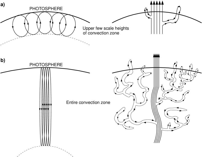
Figure 9.— Illustrations of the two basic categories of model describing the nature of the small-scale solar dynamo. The left column provides an elementary illustration of the category, and the right column illustrates a scenario in which the sub-surface field beneath a network concentration can become distorted and breach the photosphere elsewhere. a) The dynamo extends to small depths, down to the upper few scale heights of the convection zone. In this case, parts of the sub-surface field beneath a network concentration is most likely to breach the photosphere at a location near the concentration itself. b) The dynamo extends to large depths, through the entire convection zone. In this case, the breaching of the photosphere by the sub-surface field does not necessarily occur near the seed network concentration.

This leaves us with the second category, a deep small-scale dynamo, illustrated in Figure 9b as suggested by Stein et al. (2003); Stein & Nordlund (2006). A deep dynamo would allow for stretching at much larger distances, and so there would be no preference for small-scale enhancements in the proximity of the network concentration. There would also be no preference for polarity in the proximity of the network concentration due to the random tendency of the subsurface flows to breach the photosphere.

5.1. Limitations of the Result

In many cases, the network concentration appeared to be affected by nearby small-scale magnetic features. This implies that weak fields coming off or onto the network concentration can be just at the limits of visibility in the NFI magnetograms and still have an effect on the parent network concentration. While the effect of a single one of these features is small, this affect from a large number may play an important role in the network concentration evolution.

It is important to call attention to the limits of our selected parameter $P$ for comparing the new features with those of the random points. Firstly, even with a purely random distribution, we should not expect the integral of $Px_{tot}$ in Figure 7 to be zero, because of the uncertainties associated with the factors that went into its derivation. Secondly, $P$ is not effective at identifying polarity concentrations on opposite sides of a network concentration, since it averages over many variables. This is best demonstrated with a movie of NC 1029. If a network concentration had a surplus of like polarity features on one side (perhaps due to shredding) and a surplus of opposite polarity features on the other side (perhaps due to cancellation), and these features happened to be at or near the same distance from the center of the network concentration, then $Px_{tot}$, $Px_{tot}^{+}$ and $Px_{tot}^{-}$ could all be enhanced at the same distance, which would mimic the signature of subsurface field line stretching and emergence. It is therefore necessary to accompany the analysis $Px_{tot}$ with at least a visual inspection of the evolution of the network concentration (the classic balance of case studies vs. statistics).

It is important to reiterate that the features that one readily sees merging into and fragmenting from the network concentrations are not the same population as those considered in our analysis. This is because we have excluded those features born by “Fragmentation” and “Error” (see Section 3.1), which accounts for a large fraction of the features in the dataset, and an even larger fraction of the strong ones (see Lamb et al., 2010; Lamb et al., 2013). Analyzing only these small, weak features allows us to consider only the true small-scale field as observed by Hinode/NFI.

5.2. Concluding Remarks

We have conducted a statistical analysis of the birth and polarity of small-scale magnetic features in proximity to strong supergranular network concentrations. We find no observational evidence of a relationship between the network concentration and the number or polarity of features at a given distance from the network concentration. This rejects the spatially local small-scale solar dynamo hypothesis at spatial scales observable by Hinode/NFI, and we therefore conclude that the features that dominate the photospheric magnetic landscape are driven by a spatially nonlocal deep solar dynamo.

References

- Babcock (1953) Babcock, H. W. 1953, ApJ, 118, 387
- Bevington & Robinson (2003) Bevington, P. R., & Robinson, D. K. 2003, Data reduction and error analysis for the physical sciences, 3rd ed., by Philip R. Bevington, and Keith D. Robinson. Boston, MA: McGraw-Hill, ISBN 0-07-247227-8, 2003.,
- Buehler et al. (2013) Buehler, D., Lagg, A., & Solanki, S. K. 2013, A&A, 555, A33
- Cattaneo (1999) Cattaneo, F. 1999, ApJ, 515, L39
- Charbonneau (2010) Charbonneau, P. 2010, Living Reviews in Solar Physics, 7, 3
- DeForest et al. (2007) DeForest, C. E., Hagenaar, H. J., Lamb, D. A., Parnell, C. E., & Welsch, B. T., 2007, Astrophys. J., 666, 576.
- Hagenaar et al. (2008) Hagenaar, H. J., De Rosa, M. L., & Schrijver, C. J. 2008, ApJ, 678, 541
- Kosugi et al. (2007) Kosugi, T., Matsuzaki, K., Sakao, T., et al. 2007, Sol. Phys., 243, 3
- Lamb et al. (2008) Lamb, D. A., DeForest, C. E., Hagenaar, H. J., Parnell, C. E., & Welsch, B. T., 2008, Astrophys. J., 674, 520.
- Lamb et al. (2010) Lamb, D. A., DeForest, C. E., Hagenaar, H. J., Parnell, C. E., & Welsch, B. T., 2010, Astrophys. J., 720, 1405.
- Lamb et al. (2013) Lamb, D. A., Howard, T. A., DeForest, C. E., Parnell, C. E., & Welsch, B. T. 2013, ApJ, 774, 127
- Lites et al. (2008) Lites, B. W., Kubo, M., Socas-Navarro, H., et al. 2008, ApJ, 672, 1237
- Meunier et al. (2007) Meunier, N., Tkaczuk, R., Roudier, T., & Rieutord, M. 2007, A&A, 461, 1141
- Morinaga et al. (2008) Morinaga, S., Sakurai, T., Ichimoto, K., et al. 2008, A&A, 481, L29
- Parnell et al. (2009) Parnell, C. E., DeForest, C. E., Hagenaar, H. J., et al. 2009, ApJ, 698, 75
- Schrijver et al. (1997) Schrijver, C. J., Title, A. M., van Ballegooijen, A. A., Hagenaar, H. J., & Shine, R. A. 1997, ApJ, 487, 424
- Stein et al. (2003) Stein, R. F., Bercik, D., & Nordlund, Å. 2003, Current Theoretical Models and Future High Resolution Solar Observations: Preparing for ATST, 286, 121
- Stein & Nordlund (2006) Stein, R. F., & Nordlund, Å. 2006, ApJ, 642, 1246
- Stenflo (2012) Stenflo, J. O. 2012, A&A, 547, A93
- Tsuneta et al. (2008) Tsuneta, S., Ichimoto, K., Katsukawa, Y., et al. 2008, Sol. Phys., 249, 167
- Vögler & Schüssler (2007) Vögler, A., & Schüssler, M. 2007, A&A, 465, L43