Properties of $p\,$- and $f$-modes in hydromagnetic turbulence

Abstract

With the ultimate aim of using the fundamental or $f$-mode to study helioseismic aspects of turbulence-generated magnetic flux concentrations, we use randomly forced hydromagnetic simulations of a piecewise isothermal layer in two dimensions with reflecting boundaries at top and bottom. We compute numerically diagnostic wavenumber–frequency diagrams of the vertical velocity at the interface between the denser gas below and the less dense gas above. For an Alfvén-to-sound speed ratio of about 0.1, a 5% frequency increase of the $f$-mode can be measured when $k_{x}H_{p}=3$–$4$, where $k_{x}$ is the horizontal wavenumber and $H_{p}$ is the pressure scale height at the surface. Since the solar radius is about 2000 times larger than $H_{p}$, the corresponding spherical harmonic degree would be 6000–8000. For weaker fields, a $k_{x}$-dependent frequency decrease by the turbulent motions becomes dominant. For vertical magnetic fields, the frequency is enhanced for $k_{x}H_{p}\approx 4$, but decreased relative to its nonmagnetic value for $k_{x}H_{p}\approx 9$.

1 Introduction

Much of our knowledge of the physics beneath the solar photosphere is obtained from theoretical calculations and simulations. Helioseismology provides a window to measure certain properties inside the Sun; see the review by Gizon et al. (2010). This technique uses sound waves ($p\,$-modes) and to some extent surface gravity waves ($f$-modes), but the presence of magnetic fields gives rise to magneto-acoustic and magneto-gravity waves, whose restoring forces are caused by magnetic fields modified by pressure and buoyancy forces (see, e.g., Thomas, 1983; Campos, 2011). This complicates their use in helioseismology, where magnetic fields are often not fully self-consistently included. This can lead to major uncertainties.

Recent detections of changes in the sound travel time at a depth of some 60 Mm beneath the surface about 12 hours prior to the emergence of a sunspot (Ilonidis et al., 2011) have not been verified by other groups (Braun, 2012; Birch et al., 2013). Also the recent proposal of extremely low flow speeds of the supergranulation (Hanasoge et al., 2012) is in stark contrast to our theoretical understanding and poses serious challenges. It is therefore of interest to use simulations to explore theoretically how such controversial results can be understood; see, e.g., Georgobiani et al. (2007) and Kitiashvili et al. (2011) for earlier attempts trying to construct synthetic helioseismic data from simulations.

The ultimate goal of our present study is to explore the possibility of using numerical simulations of forced turbulence to assess the effects of subsurface magnetic fields on the $p\,$- and $f$-modes. Subsurface magnetic fields can have a broad range of origins. The most popular one is the buoyant rise and emergence of flux tubes deeply rooted at or even below the base of the convection zone (Caligari et al., 1995). Another proposal is that global magnetic fields are generated in the bulk of the convection zone with equatorward migration being promoted by the near-surface shear layer (Brandenburg, 2005). In this case, subsurface magnetic fields are expected to be concentrated into sunspots through local effects such as supergranulation (Stein & Nordlund, 2012) or through downflows caused by negative effective magnetic pressure instability (Brandenburg et al., 2013, 2014). The latter mechanism requires only stratified turbulence and its operation can be demonstrated and studied in isolation from other effects using just an isothermal layer. To examine seismic effects of magnetic fields on the $f$-mode, one must however introduce a sharp density drop, which implies a corresponding temperature increase. This leads us to studying a piecewise isothermal layer.

In the Sun, waves are excited by convective motions (Stein, 1967; Goldreich & Kumar, 1988, 1990). However, in an isothermal layer there is no convection and turbulence must be driven by external forcing, as it has been done extensively in the study of negative effective magnetic pressure effects. We adopt this method also in the present work, but use a rather low forcing amplitude to minimize the nonlinear effects of large Reynolds numbers and Mach numbers close to unity.

In the absence of a magnetic field, linear perturbation theory gives simple expressions for the dispersion relations of $p\,$- and $f$-modes, which are also the modes which we focus on in this work. For large horizontal wavenumbers $k_{\rm h}$, the frequencies of the solar $f$-mode have been observed to be significantly smaller than the theoretical estimates, and both line shift and line width grow with $k_{\rm h}$ (Fernandes et al., 1992; Duvall et al., 1998). Both effects are expected to arise due to turbulent background motions (Murawski & Roberts, 1993a, b; Mȩdrek et al., 1999; Murawski, 2000a, b; Mole et al., 2008). There have also been alternative proposals to explain the frequency shifts as being due to what Rosenthal & Gough (1994) call an interfacial wave that depends crucially on the density stratification of the transition region between chromosphere and corona; see also Rosenthal & Christensen-Dalsgaard (1995).

In the presence of magnetic fields, both $p\,$- and $f$-mode frequencies are affected. Nye & Thomas (1976) derive the dispersion relation for sound waves in the uniformly horizontally magnetized isothermally stratified half-space with a rigid lower boundary. In the presence of structured magnetic fields, e.g., near sunspots, a process called mode conversion can occur, i.e., an exchange of energy between fast and slow magnetosonic modes, which leads to $p\,$-mode absorption in sunspots (Cally, 2006; Schunker & Cally, 2006). The properties of surface waves in magnetized atmospheres have been studied in detail (Roberts, 1981; Miles & Roberts, 1989, 1992; Miles et al., 1992). From these results, one should expect changes in the $f$-mode during the course of the solar cycle. Such variations have indeed been observed (Antia et al., 2000; Dziembowski & Goode, 2005) and may be caused by subsurface magnetic field variations. It was argued by Dziembowski et al. (2001) that the time-variation of $f$-mode frequencies could be attributed to the presence of a perturbing magnetic field of order $20\,{\rm G}$ localized in the outer 1% of the solar radius.

The temporal variation of $f$-mode frequencies may be resolved into two components: an oscillatory component with a one-year period which is probably an artifact of data analysis resulting from the orbital period of the Earth, and another slowly varying secular component which appears to be correlated with the solar activity cycle. Subsequent work by Antia (2003) showed that variations in the thermal structure of the Sun tend to cause much smaller shifts in $f$-mode frequencies as compared to those in $p\,$-mode frequencies and as such are not effective in accounting for the observed $f$-mode variations.

Schou et al. (1997) and Antia (1998) deduced from accurately measured $f$-mode frequencies the seismic radius of the Sun. They found that the customarily accepted value of the solar radius, $695.99\,{\rm Mm}$ needs to be reduced by about $200$–$300\,{\rm km}$ to have an agreement with the observed $f$-mode frequencies. From the study of temporal variations of $f$-mode frequencies, Lefebvre & Kosovichev (2005) found evidence for time variations of the seismic solar radius in antiphase with the solar cycle above $0.99R_{\odot}$, but in phase between $0.97$ and $0.99R_{\odot}$.

The importance of using the $f$-mode frequencies for local helioseismology has been recognized in a number of recent papers (Hanasoge et al., 2008; Daiffallah et al., 2011; Felipe et al., 2012, 2013). While such approaches should ultimately be used to determine the structure of solar subsurface magnetic fields, we restrict ourselves here to the analysis of oscillation frequencies as a function of horizontal wavenumber. The purpose of the present paper is to use numerical simulations in piecewise isothermal layers to study oscillation frequencies from random forcing and to assess the effects of imposed magnetic fields on the frequencies. In the present work we restrict ourselves to the case of uniform magnetic fields and refer to the case of nonuniform fields in another paper (Singh et al., 2014), where we study what is called a fanning out of the $f$-mode.

2 Model and numerical setup

Let us consider a conducting fluid in a two-dimensional Cartesian domain with $\mbox{{\boldmath$e$}}_{x}$ and $\mbox{{\boldmath$e$}}_{z}$ denoting the unit vectors along the $x$ and $z$ directions, respectively. Let gravity be acting along $-\mbox{{\boldmath$e$}}_{z}$, with constant acceleration $g>0$. Thus we identify $x$ and $z$ as the horizontal and vertical directions, respectively. Let the domain have a large horizontal extent $L_{x}$, but a relatively small vertical extent $L_{z}\ll L_{x}$. Due to gravity, the fluid is vertically stratified. In addition it has an interface at $z=0$ with a layer of thickness $L_{z\rm u}$ above it, which is much less dense than the layer of thickness $L_{z\rm d}$ below. In the present work, we assume $L_{z\rm u}=L_{z}/6$, so $L_{z\rm d}=5L_{z}/6$. At the interface, we assume a sharp jump in density $\rho$ with ${\rho_{\rm u}}(0)\ll{\rho_{\rm d}}(0)$ along with corresponding jumps in temperature and sound speed. Such a setup may be thought of as an annular section with rectangular cross-section cut out from a star with $z=0$ being its surface. The thin layer on top represents then the rarefied hot corona and the subdomain below $z=0$ stands for the more strongly stratified uppermost part of the convection zone, which we sometimes refer to as the bulk. A schematic diagram of this setup is shown in Fig. 1.

Assuming the fluid to obey the equation of state of an ideal gas, the pressure is given by $p=(c_{p}-c_{v})\rho T=\rho c_{\rm s}^{2}/\gamma$, where $\gamma=c_{p}/c_{v}$ is the ratio of specific heats at constant pressure and volume, respectively, and $c_{\rm s}$ is the adiabatic sound speed. Assuming further both subdomains to be isothermal, the scale heights of pressure and density are constant and equal in each subdomain, $H_{p\rm d,u}=H_{\rho\rm d,u}=H_{\rm d,u}$. Thus we have

$$\rho_{\rm d,u}(z) =\rho_{\rm d,u}(0)\exp(-z/H_{\rm d,u}),$$ (1)

with

$$H_{\rm d,u} =(c_{p}-c_{v})T_{\rm d,u}/g\,$$ (2)

The abrupt changes in the thermodynamic quantities at the interface $z=0$ may be characterized by the ratio

$$q={\rho_{\rm u}}(0)/{\rho_{\rm d}}(0)=c_{\rm sd}^{2}/c_{\rm su}^{2}=H_{\rm d}/H_{\rm u}=T_{\rm d}/T_{\rm u},$$ (3)

where pressure balance ($p_{\rm d}=p_{\rm u}$) at $z=0$ has been employed. Different values of $q$ correspond to different factors by which density, temperature and sound speed change abruptly at the interface. For investigating a magnetic influence on the oscillation modes, we will also consider an augmentation of the background state by a uniform magnetic field $\bm{B}_{0}=(B_{x0},0,B_{z0})$. Note, that it does not affect the hydrostatic equilibrium.

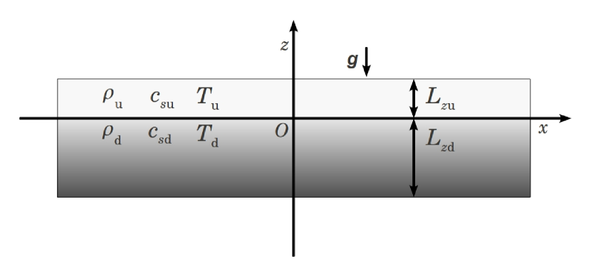
Figure 1: Geometry of the piecewise isothermal model. The layer $z>0$ is hotter than the layer $z<0$.

In Fig. 2 we show the variations of density, pressure scale height and pressure as functions of $z$, in a domain with $L_{z}/L_{0}=2\pi$ where $L_{0}=\gamma H_{\rm d}=c_{\rm sd}^{2}/g$. The solid and dashed lines correspond to $q=0.1$ and $0.01$, respectively, which are the two values employed in the present study.

Figure 2: Density (a), pressure scale height (b), and pressure (c) of the background state as functions of $z$ for $L_{z}/L_{0}=2\pi$. Solid: $q_{0}=0.1$, dashed: $q_{0}=0.01$.

Given that the oscillation modes are perturbations of the background state, we solve in our DNS the time-dependent hydromagnetic equations, extended by terms for both maintaining the background as well as exciting the oscillations. Hence the basic equations adopt the form

$$\frac{D\ln\rho}{Dt} =-\bm{\nabla}\cdot\bm{u},$$ (4)

$$\frac{D\bm{u}}{Dt} =\mbox{\boldmath$f$}{}+\bm{g}+\frac{1}{\rho}\left(\bm{J}\times\bm{B}-\bm{\nabla}p+\bm{\nabla}\cdot 2\nu\rho\bm{\mathsf{S}}\right),$$ (5)

$$T\frac{Ds}{Dt} =2\nu\bm{\mathsf{S}}^{2}+\frac{\mu_{0}\eta}{\rho}\mbox{\boldmath$J$}{}^{2}-\gamma(c_{p}-c_{v})\frac{T-T_{\rm d,u}}{\tau_{\rm c}}\,,$$ (6)

$$\frac{\partial\bm{A}}{\partial t} ={\bm{u}}\times{\bm{B}}-\eta\mu_{0}{\bm{J}},$$ (7)

where $\bm{u}$ is the velocity, $D/Dt=\partial/\partial t+\bm{u}\cdot\bm{\nabla}$ is the advective time derivative, $\bm{f}$ is a forcing function specified below, $\bm{g}=(0,0,-g)$ is the gravitational acceleration, $\nu={\rm const}{}$ is the kinematic viscosity, $\mathsf{S}_{ij}={\textstyle{1\over 2}}(u_{i,j}+u_{j,i})-{\textstyle{1\over 3}}\delta_{ij}\bm{\nabla}\cdot\bm{u}$ is the traceless rate of strain tensor, where commas denote partial differentiation, ${\bm{A}}$ is the magnetic vector potential, ${\bm{B}}=\bm{B}_{0}+\bm{\nabla}\times{\bm{A}}$ is the magnetic field, ${\bm{J}}=\mu_{0}^{-1}\bm{\nabla}\times{\bm{B}}$ is the current density, $\eta={\rm const}{}$ is the magnetic diffusivity, $\mu_{0}$ is the vacuum permeability, and $T$ is the temperature. For our purposes, viscous and Ohmic damping of the modes are parasitic effects, so we have included them only to ensure numerical stability and chosen $\nu$ and $\eta$ as small as possible. For the same reason, bulk viscosity was omitted. The boundaries at $z=-L_{z\rm d},L_{z\rm u}$ are chosen to be impenetrable, stress-free, and perfectly conducting, while at the $x$ boundaries periodicity is enforced.

The last term in Eq. (6), being of relaxation type, is to guarantee that the temperature is on average constant in either subdomain and equal to $T_{\rm d}$ and $T_{\rm u}$, respectively. For too high temperatures cooling is provided, but heating for too low ones. Due to permanent viscous and Ohmic heating, however, cooling is necessary on average. In test runs we found that the relaxation term can be omitted in the lower part of the domain as long as the dissipation rate is sufficiently small. Accordingly, the temperature in the lower subdomain is set by the initial condition defined by the piecewise isothermal $z$ profiles with the desired value of $q$; see Fig. 2. For numerical reasons, the jumps at $z=0$ were smoothed out over a few grid cells. Note that without the relaxation term in $z<0$, there is a slow drift in the $xt$ averages of density and temperature, reflected by a deviation of the actual value of $q$, calculated with these averages, from its initial value, which we now call $q_{0}$. For the relaxation rate $\tau_{\rm c}^{-1}$ (in $z>0$) we choose $0.5\,g/c_{\rm sd}$ throughout this paper. On average, this corresponds to about $0.2u_{\rm rms}k_{\rm f}$.

We provide a weak stochastic forcing $f$ in an isotropic and homogeneous fashion, at a length scale, which is much shorter than the box dimensions, for details see Brandenburg (2001). The average forcing wavenumber $k_{\rm f}$ defines the energy injection scale $l_{\rm f}=2\pi/k_{\rm f}$ of the flow. In the present study, we have used $k_{\rm f}/k_{1}=20$, where $k_{1}=2\pi/L_{x}$ is the lowest wavenumber in the domain. Normally the forcing is specified to act exclusively in the lower subdomain, but we also compare with the case when it is provided in the entire domain. These two choices gave basically identical results, most likely due to the weakness of the forcing and the fact that the sound speed is high in the upper part and disturbances are quickly propagated.

We compute the root-mean-squared value of the turbulent motion from regions below the interface ($z<0$), which we expect to be physically most relevant for our purpose and denote it by $u_{\rm rms,d}$. Let us define corresponding fluid Reynolds and Mach numbers of the flow as

$${\rm Re}\;=\;\frac{u_{\rm rms,d}}{\nu k_{\rm f}},\qquad{\rm Ma}\;=\;\frac{u_{\rm rms,d}}{c_{\rm sd}}.$$ (8)

For characterizing the forcing strength, it is useful to employ the dimensionless quantity

$${\cal F}\;=\;f_{0}\,{\rm Rc}\;=\;f_{0}\frac{c_{\rm sd}}{\nu\,k_{\rm f}}\;,$$ (9)

where $f_{0}$ is a dimensionless measure of the forcing amplitude (non-dimensionalized by $\sqrt{k_{\rm f}c_{\rm sd}^{3}/\delta t}$ with the timestep of the numerical integration $\delta t$, Brandenburg, 2001). ${\rm Rc}$ may be thought of as the fluid Reynolds number defined with respect to the sound speed $c_{\rm sd}$. The random forcing is expected to excite acoustic, internal gravity, and surface waves, referred to as $p\,$-, $g\,$-, and $f$-modes, respectively. Although our primary goal is to study the properties of the $f$-mode under a variety of physical conditions, we also turn to $p\,$-modes in some detail, while $g\,$-modes are inspected only at a qualitative level.

It is customary to show the presence of these modes in a $k_{x}$–$\omega$ diagram, to which we refer in the following simply as $k\omega$ diagram. It shows the amplitude of the Fourier transform of the vertical velocity $u_{z}$ as a function of $k_{x}$ and $\omega$. Here, we take $u_{z}$ from the interface at $z=0$, where the $f$-modes are expected to be most prominent. By Fourier transforming $u_{z}(x,0,t)$ in $x$ and $t$, we obtain the quantity $\hat{u}_{z}(k_{x},\omega)$. Results are presented in terms of the dimensionless wavenumber $\widetilde{k}_{x}$ and angular frequency $\widetilde{\omega}$,

$$\widetilde{k}_{x}=k_{x}L_{0},\quad\widetilde{\omega}=\frac{\omega}{\omega_{0}},\quad\omega_{0}=\frac{g}{c_{\rm sd}},$$ (10)

where $\omega_{0}$, being twice the Lamb acoustic cutoff frequency of the bulk,

$$\omega_{c}=g/2c_{\rm sd}=c_{\rm sd}/2L_{0},$$ (11)

provides a natural time scale. As $\hat{u}_{z}(k_{x},\omega)$ has the dimension of length squared, we construct the dimensionless quantity

$$\widetilde{P}(\omega,k_{x})\;=\;\frac{|\hat{u}_{z}|}{{\cal D}^{2}}\;=\;\frac{|\hat{u}_{z}|}{L_{0}^{2}}\,\frac{c_{\rm sd}^{2}}{u_{\rm rms,d}^{2}},$$ (12)

where ${\cal D}=u_{\rm rms,d}/\omega_{0}$ characterizes the distance travelled with speed $u_{\rm rms,d}$ in an acoustic time $\omega_{0}^{-1}$. Note that ${\cal D}=\mbox{\rm Ma}L_{0}$ is smaller than $L_{0}$ for our values of Ma.

3 Non-magnetic case

We first study mode excitation in the absence of an imposed magnetic field by performing simulations for three different extents ($L_{x}\times L_{z}$) of the domain, while keeping $q_{0}=0.1$ and ${\cal F}=0.05$ fixed; see Table 1. The different box sizes were chosen to compare properties such as frequency shifts and line broadening of the $p\,$- and $f$-modes.

The $k\omega$ diagrams for Runs A ($L_{z}=2\pi$) and B ($L_{z}=\pi$) are shown in Figs. 3 and 4, where modes of all types ($p$, $g$ and $f$) clearly appear. The multiple curves to the left of the long-dashed line belong to the $p\,$-modes, the curve just below the short-dashed line corresponds to the $f$-modes and the curves further below indicate $g\,$-modes. Especially in the lower left corner of Fig. 4 one can distinguish several different branches.

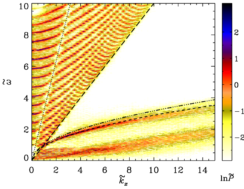
Figure 3: $k\omega$ diagram for Run A ($8\pi\times 2\pi$ domain, no magnetic field). The dotted and long dashed lines shows $\omega=c_{\rm su}k_{x}$ and $\omega=c_{\rm sd}k_{x}$, respectively. The dash-triple-dotted and dashed curves show $\omega_{\rm f0}$ and $\omega_{\rm f}$, respectively.

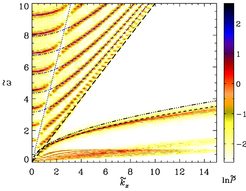
Figure 4: Same as Fig. 3 but for Run B ($8\pi\times\pi$, no magnetic field). Dash-dotted (blue): some of the estimated $p\,$-modes according to Eqs. (13) and (15).

Table 1: Summary of simulations without magnetic field, $q_{0}=0.1$ and ${\cal F}=0.05$.

Run	Domain	Grid600	$q$	${\rm Re}$	${\rm Ma}$
A	$8\pi\times 2\pi$	$1024\times 600$	0.093	1.94	0.004	(Fig. 3)
B	$8\pi\times\pi$	$1024\times 300$	0.092	0.95	0.002	(Fig. 4)
C	$4\pi\times\pi$	$512\times 300$	0.091	0.93	0.002

3.1 $p\,$-modes

The $p\,$-modes, also known as pressure modes, are acoustic waves that are trapped in a resonant cavity. In a stratified isothermal medium (without interface), their dispersion relation is in two dimensions approximately given by

$$\omega^{2}\approx\omega_{c}^{2}+c_{\rm s}^{2}\left(k_{x}^{2}+k_{z}^{2}\right),$$ (13)

where $k_{x}$ and $k_{z}$ adopt discrete values depending on the extent of the cavity and $\omega_{c}=g/2c_{\rm s}$ is again the Lamb acoustic cutoff frequency (11). In Eq. (13) the contribution $N^{2}/\omega^{2}$ with the Brunt-Väisälä frequency $N=(\gamma-1)^{1/2}g/c_{\rm s}$ (Stein & Leibacher, 1974) has been ignored, as typically $\omega\gg N$ for acoustic modes. Impenetrable $z$ boundaries let the waves be standing in the $z$ direction, whereas periodic $x$ boundaries allow them to travel in the $x$ direction. For the vertical wavenumber $k_{z}$, the discrete values $n\pi/L_{z}$ with integer $n$ are possible and thus from Eq. (13) a set of eigenvalue curves $\omega_{n}(k_{x})$ can be formed. In a $k\omega$ diagram they are bound from below by the asymptotic line $\omega=c_{\rm s}k_{x}$.

Turning to our two-layer setup and inspecting the $k\omega$ diagrams in Figs. 3 and 4, we note that the asymptotic line is now found to be $\omega=c_{\rm sd}k_{x}$, just as the cavity were given by the lower subdomain. As a major difference from the picture expected for a single layer, gaps coinciding with apparent discontinuities in the $\omega_{n}(k_{x})$ curves occur. They seem to line up along

$$\omega=c_{\rm su}k_{x},$$ (14)

which would be the asymptotic line if the cavity were given by the upper subdomain alone. The higher complexity of the $k\omega$ diagram in comparison with the single layer is due to the existence of three different families of $p$-modes instead of only one: while in a single isothermal layer all standing waves have the $z$ dependence $\exp(-\kappa z)\sin(k_{z}z+\phi)$, the two-layer setup allows additionally waves which are purely exponential (or evanescent) in one of the subdomains and (damped) harmonic in the other. Those which are evanescent in the bulk are in Hindman & Zweibel (1994) identified with the line (14) and called “$a$-modes”, although the actual mode frequencies follow a pattern that is referred to as “avoided crossings” with the $p$- and $f$-modes. In the following we refer to this line as separatrix. The suppression of the mode amplitude around the separatrix is, however, not explained by ideal linear theory.

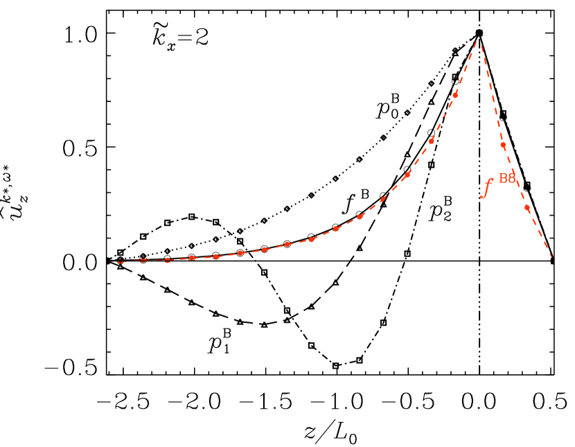
Figure 5: Eigenfunctions of the $f$- and the first three $p$-modes ($p_{0}$, $p_{1}$ and $p_{2}$) at $\widetilde{k}_{x}=2$. Black curves correspond to Run B, whereas the red curve (with filled circles) shows the $f$-mode corresponding to Run B8, which has horizontal magnetic field. The vertical (dash-dots) line shows the location of the interface.

To determine the shape of the $f$- and $p$-mode eigenfunctions, we derived them from the $z$ dependent spectrum of $u_{z}$ by selecting $\widetilde{k}_{x}=2$ and $\widetilde{\omega}=1.31,\,2.09,\,2.77,\,3.67$ corresponding to the $f$-mode and the first three $p$-modes, $p_{0,1,2}$, respectively. The result is shown in Fig. 5, corresponding to Runs B and B8. For $p_{0}$ the eigenfunction is approximately a (damped) quarter wave with a node at the bottom and a maximum at the interface. Accordingly, we make the following tentative ansatz for the vertical wavenumbers (analogous to those of organ pipes):

$$k_{z}\;=\;\frac{\pi(n+1/2)}{L_{z\rm d}}\;,\quad n=0,1,2,\ldots\,,$$ (15)

where $n$ is the number of nodes in the $z$ direction. It is interesting to recall here Duvall’s law, which was applied to the solar observations (Duvall, 1982):

$$k_{z}\;=\;\frac{\pi(n_{D}+\alpha)}{L_{z\rm d}}\;,\quad n_{D}=1,2,3,\ldots\,.$$ (16)

The fundamental mode, with radial node number $n_{D}=0$, was excluded from this formula, and the best fit value for $\alpha$ was found to be $\approx 3/2$, which is intended to account for the fact that the interface is “soft” instead of rigid. In general, $\alpha$ has to be considered frequency dependent (see Gough, 1987; Christensen-Dalsgaard, 2003). We also note that the possibility of misidentification of the radial node number ($n_{D}$) was explicitly discussed in Duvall (1982).

Given that our model setup is quite different from the real Sun, we should perhaps not seek direct comparison between Eqs. (15) and (16), although it is noteworthy to mention that, as shown in Fig. 5, both the $f$- and the $p_{0}$- mode, corresponding to $n=0$ in Eq. (15), do not have any node within the bulk. Hence one could ask whether a qualitative distinction between those modes is tenable. This might help resolving the observational issue of proper identification of the radial node number, when the eigenfunctions of various trapped modes are not readily accessible. Also, note that Eqs. (15) and (16) are equivalent if $\alpha=1/2$ and $n_{D}$ is allowed to include the value $0$, too.

In Figs. 6 and 7 we plot the dimensionless spectral mode amplitude $\widetilde{P}$ as a function of $\widetilde{\omega}$ for $\widetilde{k}_{x}=2$ and $4$, respectively, for Runs A, B and C; see also Table 1. The dash-dotted (blue) and dashed (red) lines mark the locations of the $f$- and $p\,$-modes as expected from Eq. (17) and Eq. (15), respectively. The group of peaks to the left of the $f$-mode indicate $g\,$-modes. The (blue) dotted lines mark the $\omega=c_{\rm su}k_{x}$ line, which is shown by the dotted line in Figs. 3 and 4.

We find that various peaks of the $p\,$-mode appear at the locations predicted by Eq. (15), although there are some slight frequency shifts, as may be seen from Figs. 6 and 7. We also note that the frequency shift changes sign across the $\omega=c_{\rm su}k_{x}$ line, shown by blue dotted lines in Figs. 6 and 7. Comparing the different panels in each of Figs. 6 and 7, we first note that the number of $p\,$-mode peaks are two times smaller in Runs B and C compared to Run A. This is expected as the vertical extent ($L_{z}$) in Run A is twice as large as in Runs B and C. From Fig. 6, corresponding to $\widetilde{k}_{x}=2$, we see that the dimensionless mode amplitudes $\widetilde{P}(\omega)$ of the corresponding peaks of the $p\,$-mode are in all three cases comparable, even though the domain sizes are different. The same holds true for Fig. 7 corresponding to $\widetilde{k}_{x}=4$, although the mode amplitudes have generally decreased for the $\widetilde{k}_{x}=4$ case. We find that the Mach number in the lower subdomain decreases by the same factor as we decrease the vertical extent of the cavity in spite of the same strength of forcing in all cases (see Table 1 and note that ${\cal F}=0.5$ for all three cases). This might be due to the fact that a larger number of $p\,$-modes are present in a larger cavity (in our case, twice as many), thus contributing to the random motion, which increases the value of ${\rm Ma}$.

Frequency shifts of the $p\,$-modes due to the presence of a hot layer above the cavity have been calculated in Hindman & Zweibel (1994); Dzhalilov et al. (2000). The first of these papers deals with $p$-modes in an infinitely extended volume filled with a gas obeying an adiabatic equation of state. Temperature and hence sound speed are considered height dependent with a minimum close to the solar surface. Eigensolutions are obtained by requiring regularity at infinity. The second work employs a piecewise isothermal three-layer model in which between two layers, allowing sound waves to propagate, a further one is embedded where the waves are evanescent. This setup resembles the conditions in the neighbourhood of the temperature minimum in the lower chromosphere. It is demonstrated that, if the cool layer is sufficiently shallow, $p$-modes can “tunnel” through it from one propagation layer to the other. The results of both papers cannot easily be applied to our two-layer model.

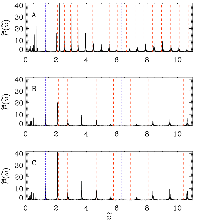
Figure 6: $\widetilde{P}(\widetilde{\omega};\widetilde{k}_{x}=2)$ as a function of $\widetilde{\omega}$ in the absence of a magnetic field for Runs A, B and C (top to bottom); see Table 1. Dash-dotted (blue) and dashed (red): theoretical locations of the $f$- and $p\,$-modes according to Eqs (17), (13) and (15), respectively. (Blue) dotted lines: position of the separatrix (14) shown dotted in the $k\omega$ diagrams (see e.g., Fig. 3).

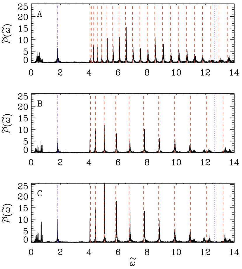
Figure 7: Same as Fig. 6, but for $\widetilde{k}_{x}=4$.

3.2 $f$-mode

The classical $f$-mode, also known as the fundamental mode, is a surface wave which exists due to a discontinuity in the density. In the absence of a magnetic field, the dispersion relation for the $f$-mode is given by (see, e.g., Gough, 1987; Campbell & Roberts, 1989; Evans & Roberts, 1990)

$$\omega_{\rm f}^{2}=gk_{x}\,\frac{1-q}{1+q},\quad\omega_{\rm f0}^{2}=gk_{x},$$ (17)

where $\omega_{\rm f0}$ is the frequency in the limit when ${\rho_{\rm u}}=0$, that is, $q=0$. The dashed and dash-triple-dotted curves in Figs. 3 and 4 show $\omega_{\rm f}$ and $\omega_{\rm f0}$, respectively. For linear perturbations, the dispersion relation as given by Eq. (17) is independent of the background stratification and the thermodynamic properties of the fluid. Consequently the $f$-mode, in contrast to the $p\,$-modes, was traditionally expected to be less of diagnostic value, and received less attention. However, observations (Fernandes et al., 1992; Duvall et al., 1998) revealed significant deviations of the frequencies of the solar $f$-modes from the simple relation given in Eq. (17), so their diagnostic importance grew significantly (Rosenthal & Gough, 1994; Rosenthal & Christensen-Dalsgaard, 1995; Ghosh et al., 1995; Mȩdrek et al., 1999; Murawski, 2000a, b). Attempts were made to explain the frequency shifts of the high spherical harmonic degree solar $f$-modes by considering them as interfacial waves, which propagate at the chromosphere-corona transition (Rosenthal & Gough, 1994; Rosenthal & Christensen-Dalsgaard, 1995). The other hypothesis mentioned earlier invokes frequency shifts and line broadening of the $f$-mode due to the turbulent motions (Murawski & Roberts, 1993a, b; Mȩdrek et al., 1999; Murawski, 2000a, b). It is at present unclear which of these explanations is more relevant for the Sun.

In our simulations, the $f$-mode frequencies lie significantly below $\omega_{\rm f0}$ and are much closer to $\omega_{\rm f}$ for small $k_{x}$ values (see Figs. 3 and 4). However, for large values of $k_{x}$ the line center falls progressively below the theoretically expected $\omega_{\rm f}$ curve. We also notice a line broadening for large values of $k_{x}$. It is discussed in earlier works (Mȩdrek et al., 1999; Murawski, 2000a, b) that, for large horizontal wavenumbers, both frequency shift and line broadening may be caused by incoherent background motions that we simply refer to as “turbulence”. However, it may be more appropriate to characterize shift and broadening as finite Mach number effects.

Figure 8: Line profiles of the $f$-mode at $\widetilde{k}_{x}=6$ in the absence of a magnetic field for Runs A and B. Dotted: data from DNS, solid: Gaussian fit.

In order to quantify our results, we focus on the line profiles of the $f$-mode under various physical conditions. To that end, we fit the quantity $\widetilde{P}(\omega,k_{x})$ for a fixed value of $k_{x}$ to a Gaussian by a robust nonlinear least squares method using publicly available standard procedures (Markwardt, 2009). The fit parameters include the central frequency ${\omega_{{\rm f}\#}}$, the line width, the peak value and the vertical shift. In Fig. 8, dotted lines indicate $\widetilde{P}(\omega,k_{x})$ at $\widetilde{k}_{x}=6$ for Runs A and B, while the Gaussian fit is given by bold lines. The vertical shift characterizes the ‘turbulence continuum’, whereas the Gaussian profile represents the mode proper.

Let us denote the numerical estimate of the line center from the fit by ${\omega_{{\rm f}\#}}$ and characterize the relative frequency shift by

$$\frac{\delta\omega_{\rm f}^{2}}{\omega_{\rm f}^{2}}\equiv\frac{{\omega_{{\rm f}\#}^{2}}-\omega_{\rm f}^{2}}{\omega_{\rm f}^{2}}$$ (18)

as a measure of the departure of the detected $f$-mode frequency from its theoretical value (17). For characterizing the amplitude of an $f$-mode we define the normalized mode mass as the area under the Gaussian fit after subtracting the continuum:

$$\mu_{\rm f}\;=\;\frac{1}{\nu_{\rm t}}\int\Delta|\hat{u}_{z}|\,\mathrm{d}\omega,$$ (19)

where $\Delta|\hat{u}_{z}|$ denotes the excess over the ‘continuum’ and $\nu_{\rm t}=u_{\rm rms,d}/3k_{\rm f}$ is an estimate for the turbulent viscosity, which has been used on purely dimensional grounds. The dimensionless measure of the linewidth of an $f$-mode at a central frequency ${\omega_{{\rm f}\#}}$ is defined by

$$\Gamma_{\rm f}\;=\;\frac{\Delta\omega_{\rm FWHM}}{{\omega_{{\rm f}\#}}},$$ (20)

where $\omega_{\rm FWHM}$ is the full width at half maximum of the line profile. Frequency shift, mode mass and linewidth will now be employed to analyse DNS under a variety of physical conditions.

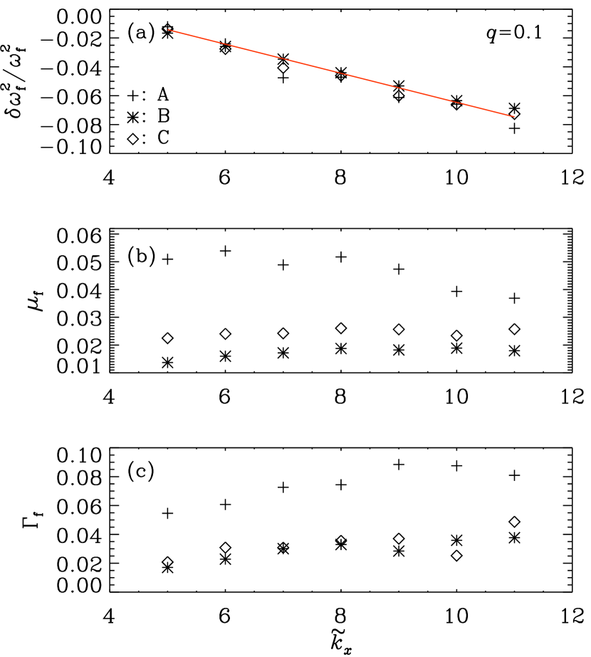
Figure 9: Relative frequency shift (a), mode mass (b), and linewidth (c) of the $f$-mode as a function of $\widetilde{k}_{x}$ in the absence of a magnetic field. Symbols ‘$+$’, ‘$\ast$’, and ‘$\diamond$’: Runs A, B and C, respectively (see Table 1) and the red line represents an approximate fit to the data.

Noting the fact that the Mach number is larger in a deeper domain (see Table 1), we find that (i) the peak value of $\widetilde{P}(\widetilde{\omega})$ decreases with increasing $k_{x}$ and is larger for a shallower domain at any value of $k_{x}$ than for a deeper one, (ii) the linewidth of the $f$-mode increases with $k_{x}$ and is smaller for a shallower domain.

In Fig. 9 we show the dependencies of $\delta\omega_{\rm f}^{2}/\omega_{\rm f}^{2}$, $\mu_{\rm f}$, and $\Gamma_{\rm f}$ on $k_{x}$ for the Runs A, B and C, which have different domain sizes and Mach numbers (see Table 1). Remarkably, the values of $\delta\omega_{\rm f}^{2}/\omega_{\rm f}^{2}$ for Runs A, B and C almost coincide in Fig. 9(a) and show a linearly decreasing trend with $k_{x}$, indicated by the red line with slope $\sim-0.01$. However, such $k_{x}$-dependent frequency shifts of the $f$-mode are expected both from the influence of turbulent motions (Mȩdrek et al., 1999; Murawski, 2000a, b; Mole et al., 2008, where shifts are linear in $k$), as well as for interfacial waves propagating in the transition region between chromosphere and corona (Rosenthal & Gough, 1994; Rosenthal & Christensen-Dalsgaard, 1995). By comparison, purely viscous effects proportional to $\nu k^{2}$ would yield a relative frequency shift $\delta\omega^{2}/\omega^{2}\approx 2\nu k_{x}^{3/2}/\sqrt{g}$, which is around $10^{-3}$ for $\widetilde{k}_{x}=10$. Although this correction would be linear in $k_{x}$, just like in our simulations, it is clearly negligible. Note also that the mode mass decreases only slightly with $k_{x}$ for the deeper domain, while for the shallower one, however, it stays nearly constant. The linewidth increases in all cases somewhat with $k_{x}$. Also, both $\mu_{\rm f}$ and $\Gamma_{\rm f}$ are considerably smaller in the shallower domains of Runs B and C, compared to the deeper one of Run A, but it is worthwhile to note that the corresponding Mach numbers are also smaller, as will be discussed in Sect. 4.2. We return to this in the next section, where we show that in our simulations magnetic fields also affect the Mach number and thus the mode mass.

3.3 $g\,$-modes

When inspecting Figs. 3 and 4, we note that the $g\,$-modes appear sharper in the latter case (Run B, shallower domain) compared to the former (Run A, deeper domain). Individual $g\,$-modes can be identified for small values of $\widetilde{k}_{x}$ up to $\tilde{k}_{x}=4$ and 6, respectively. The envelope surrounding the g modes shows saturation for $\widetilde{k}_{x}\lesssim 7$ and 4, respectively. For larger values of $\widetilde{k}_{x}$, the envelope seems to continue with a mild increase in frequency. Although this effect is more clearly seen for the deeper domain (Fig. 3), in both cases the center line is nevertheless compatible with a straight line going through zero with almost the same slope and almost the same intersection point, $(\widetilde{k}_{x},\widetilde{\omega})\approx(7,0.8)$, with the saturated part of the envelope. The latter can be explained from the analysis of a single isothermal layer, applied to the lower subdomain. A further linear increase of the $g$-mode frequencies is possible due to the existence of $g$-modes in the upper subdomain of a two-layer setup; see Hindman & Zweibel (1994). These are also expected to saturate at some constant, but for much higher values of $k_{x}$. Wagner & Schmitz (2007), while studying the effect of a hot layer above the photosphere, find that there is a continuous spectrum below the $f$-mode, with frequencies linearly increasing with $k_{x}$ for intermediate values of $\widetilde{k}_{x}$.

4 Horizontal magnetic field

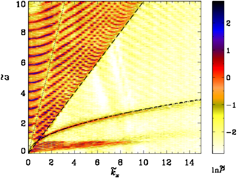
Figure 10: $k\omega$ diagram for Run A2 with horizontal magnetic field. The dotted and long dashed lines show $\omega=c_{\rm su}k_{x}$ and $\omega=c_{\rm sd}k_{x}$, respectively. The dash-triple-dotted and dashed curves (nearly on top of each other as $B_{x0}$ is small; but cf. Fig. 11) show $\omega_{\rm f}$ and $\omega_{\rm fm}$, respectively; see Table 2.

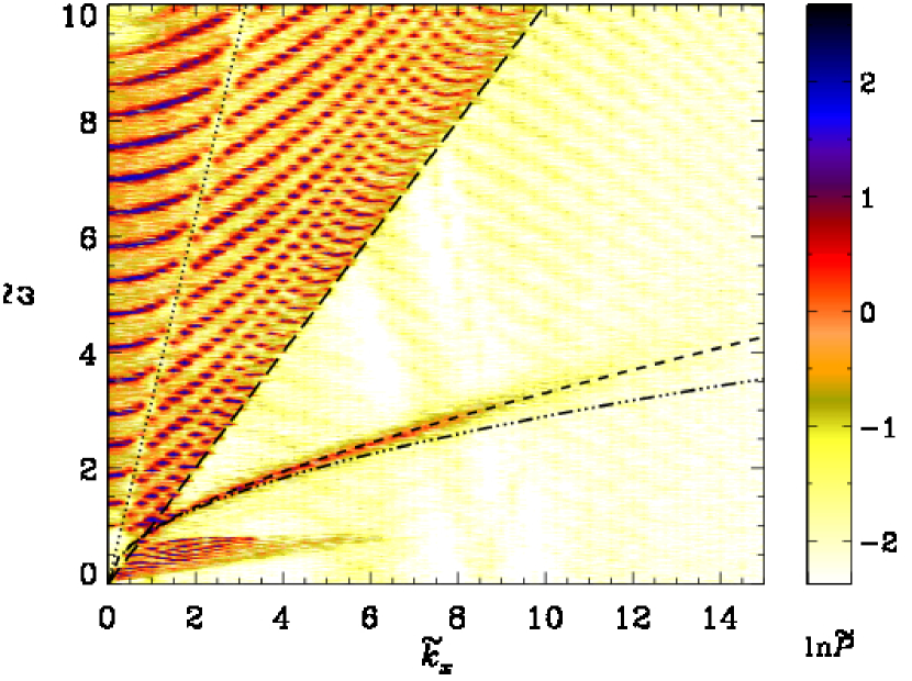
Figure 11: Same as Fig. 10, but for Run A5 with a 5 times stronger magnetic field.

We impose a uniform horizontal magnetic field $(B_{x0},0,0)$ in the entire domain and study its effect on the different modes for varying domain sizes, density jumps, and field strengths $B_{x0}$, with a focus on its effect on the $f$-mode. Details of the simulations discussed in this section are summarized in Table 2, where we have employed Alfvén velocities which are different in the bulk and the corona according to

$$v_{{\rm A}x\,{\rm d,u}}\,=\,B_{x0}/\sqrt{\mu_{0}\rho_{\rm d,u}(0)}.$$ (21)

On the other hand, the ratio $v_{{\rm A}x}/c_{\rm s}$ is approximately the same above and below the interface. So, for definitiveness, we denote by $v_{\rm A}/c_{\rm s}$ in the following the average of both values.

The $k\omega$ diagrams for some of our runs are shown in Figs. 10–14. The $p\,$-, $g\,$- and $f$-modes appear clearly in all the diagrams and are seen to be affected by the magnetic field. As before, the dotted and long-dashed lines show $\omega=c_{\rm su}k_{x}$ and $\omega=c_{\rm sd}k_{x}$, respectively.

Table 2: Summary of simulations with horizontal magnetic field. Runs A1–A6h: $L_{z}/L_{0}=2\pi$; Runs B8 and B8h: $L_{z}/L_{0}=\pi$.

Run	Grid	$q_{0}$	$q$	$v_{{\rm A}x\rm d}/c_{\rm sd}$	$v_{{\rm A}x\rm u}/c_{\rm su}$	${\rm Ma}$	${\rm Re}$	${\cal F}$
A1	$1024\times 600$	0.1	0.097	0.004	0.004	0.0030	0.71	0.025
A2	$1024\times 600$	0.1	0.091	0.025	0.025	0.0032	0.61	0.020	(Fig. 10)
A3	$1024\times 600$	0.1	0.095	0.042	0.041	0.0027	0.52	0.020
A3’	$1024\times 600$	0.1	0.093	0.042	0.041	0.0028	0.54	0.020
A4	$1024\times 600$	0.1	0.095	0.106	0.102	0.0029	0.68	0.025
A5	$1024\times 512$	0.1	0.089	0.124	0.123	0.0032	0.76	0.025	(Fig. 11)
A3h	$1024\times 600$	0.01	0.0110	0.042	0.039	0.0014	0.27	0.020	(Fig. 12)
A5h	$1024\times 512$	0.01	0.0091	0.119	0.116	0.0021	0.50	0.025
A6h	$1024\times 512$	0.01	0.0096	0.162	0.156	0.0015	0.34	0.020	(Fig. 13)
B8	$1024\times 300$	0.1	0.099	0.296	0.283	0.0016	0.78	0.050	(Fig. 14a)
B8h	$1024\times 300$	0.01	0.0098	0.290	0.273	0.0015	0.71	0.050	(Fig. 14b)

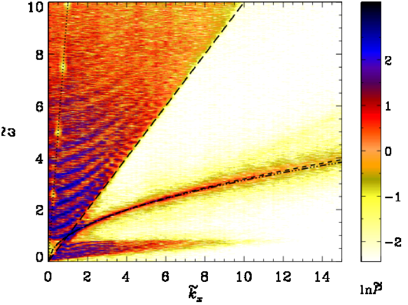
Figure 12: Same as Fig. 10, but for Run A3h with hotter corona.

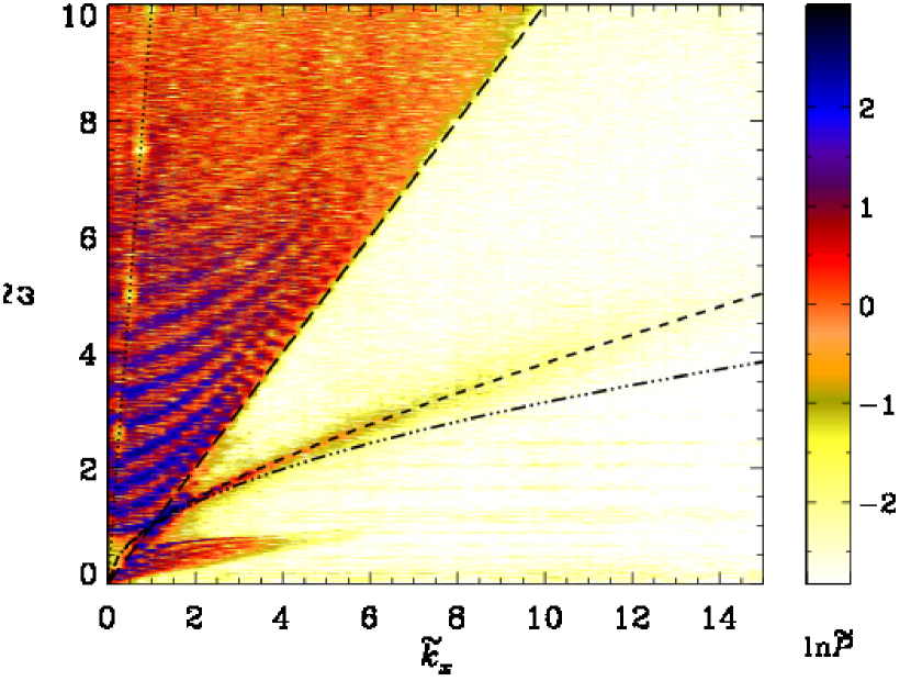
Figure 13: Same as Fig. (12), but for Run A6h with a stronger magnetic field.

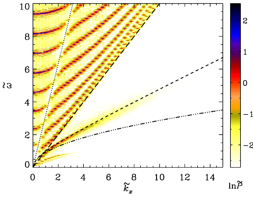
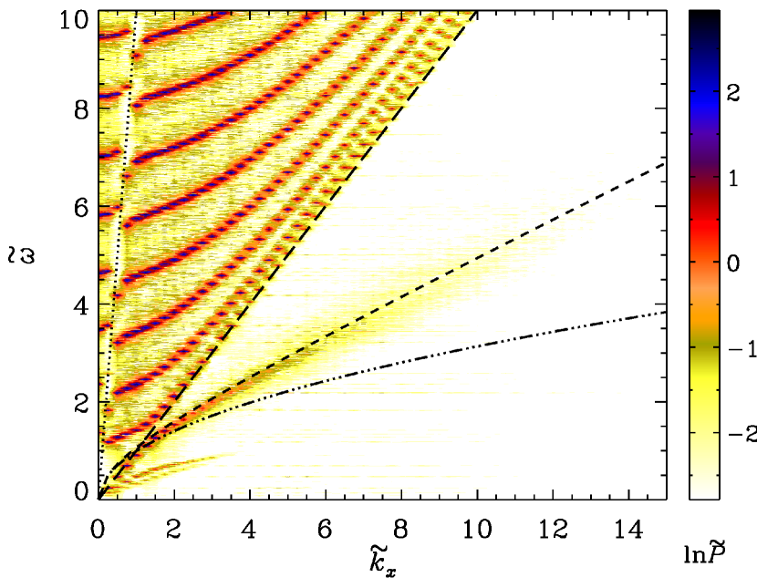
Figure 14: $k\omega$ diagrams for a domain $8\pi\times\pi$ and a magnetic field with $v_{{\rm A}x\rm d}/c_{\rm sd}=0.29$. Top: Run B8, $q=0.099$; bottom: Run B8h, $q=0.0098$.

4.1 $p\,$-modes

The results of Nye & Thomas (1976) demonstrate that already for small values of the parameter $v_{\rm A}(0)/c_{\rm s}$ there can be a noticeable influence on the eigenfrequencies (see their Fig. 1). However, it has to be considered that $v_{\rm A}(z)/c_{\rm s}$ grows to infinity due to the exponential decrease of density with height and the lack of an upper boundary in their setup. Hence, their findings cannot directly be transferred to our model of finite thickness. Therefore we restrict ourselves to a comparison with the non-magnetic case to infer the magnetically induced departures of frequency, mode amplitude, mode mass, and line width.

In the $k\omega$ diagram, such as Fig. 14, we notice again the apparent gap in the $p\,$-mode spectrum coinciding with the separatrix $\omega=c_{\rm su}k_{x}$ (dotted). In Fig. 15 we plot $\widetilde{P}$ as a function of $\widetilde{\omega}$ at $\widetilde{k}_{x}=2$ for six cases with different field strengths, domain depths, and the two $q$ values, $0.1$ and $0.01$; for details see Table 2. The dash-dotted blue lines show the theoretically expected locations of the non-magnetic $f$-mode; see Eq. (17). The group of peaks to the left of the $f$-mode are the $g\,$-modes, whereas those to the right are $p\,$-modes. The blue dotted lines mark the position of the separatrix shown dotted in the $k\omega$ diagrams. The red lines show the locations of theoretically expected $p\,$-modes corresponding to the non-magnetic case; see Eqs. (13) and (15).

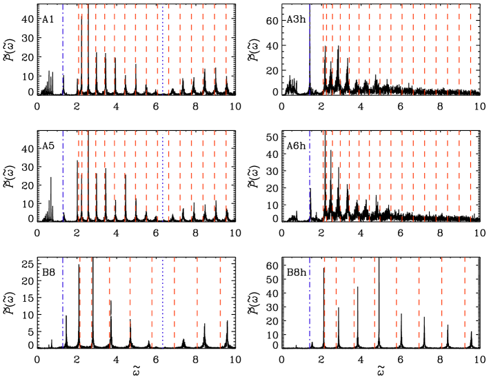
Figure 15: $\widetilde{P}(\widetilde{\omega};\widetilde{k}_{x}=2)$ as function of $\widetilde{\omega}$ with horizontal magnetic field for Runs A1 (a), A5 (c) and B8 (e), each with $q_{0}=0.1$, whereas $q_{0}=0.01$ for Runs A3h (b), A6h (d) and B8h (f); see Table 2. Dash-dotted (blue) and dashed (red) lines: theoretically expected locations of the $f$- and $p\,$-modes, respectively. Blue dotted lines: position of the $\omega=c_{\rm su}k_{x}$ line, shown dotted in the $k\omega$ diagrams (see e.g., Fig. 11).

Looking at different panels of Fig. 15 and also making some comparisons with the non-magnetic case in Fig. 6, we notice that the frequencies of the individual peaks of the $p\,$-modes are not much affected by the presence of magnetic fields when $q_{0}=0.1$. However, for the stronger density jump at the interface ($q_{0}=0.01$), slight frequency shifts of the $p\,$-modes may be seen from the right panels of Fig. 15. The mode amplitudes also seem to have increased compared to the corresponding cases with $q_{0}=0.1$.

According to the work of Hindman & Zweibel (1994), albeit in the absence of a magnetic field, the $p\,$-modes are expected to be strongly affected by a hot outer corona. Indeed, we see from our results that for the larger coronal temperature, there is a noticeable effect on the $p\,$-modes, which might not be connected with the magnetic field, at least in the parameter regimes explored. Also, for higher coronal temperatures, the high frequency peaks appear sharp in a shallower domain (Run B8h), while for the deeper domain (Runs A3h and A6h) the data look more noisy.

4.2 $f$-mode

Given that the Alfvén speeds in the layers above and below the interface are different due to the density jump at $z=0$, our setup mimics the ‘single magnetic interface’ of Roberts (1981), Miles & Roberts (1989, 1992), and Miles et al. (1992). It is capable of supporting a surface wave which, in the absence of gravity, propagates with the phase speed $c_{\rm fm}$, given by (Kruskal & Schwarzschild, 1954; Dungey & Loughhead, 1954; Gerwin, 1967; Miles & Roberts, 1989)

$$c_{\rm fm}^{2}=\frac{{\rho_{\rm u}}v_{{\rm A}x\rm u}^{2}+{\rho_{\rm d}}v_{{\rm A}x\rm d}^{2}}{{\rho_{\rm u}}+{\rho_{\rm d}}}=\frac{2{\rho_{\rm u}}v_{{\rm A}x\rm u}^{2}}{{\rho_{\rm d}}+{\rho_{\rm u}}}=\frac{2{\rho_{\rm d}}v_{{\rm A}x\rm d}^{2}}{{\rho_{\rm d}}+{\rho_{\rm u}}};$$ (22)

thus, $v_{{\rm A}x\rm d}\leq c_{\rm fm}\leq v_{{\rm A}x\rm u}$. We note that this expression is valid for an incompressible fluid. A more general result is given by Roberts (1981), but in our parameter regime the difference is small. The presence of gravity modifies the dispersion relation (Chandrasekhar, 1961; Roberts, 1981; Miles & Roberts, 1989, 1992; Miles et al., 1992):

$$\omega_{\rm fm}^{2}=c_{\rm fm}^{2}k_{x}^{2}+gk_{x}\frac{1-q}{1+q},$$ (23)

where $c_{\rm fm}^{2}k_{x}^{2}$ always adds to the (squared) frequency of the classical $f$-mode given by Eq. (17).

In Figs. 10–14, the dash-triple-dotted and dashed curves show the expected $f$-mode frequencies in the absence and presence of a horizontal magnetic field, given by $\omega_{\rm f}$ and $\omega_{\rm fm}$, respectively; see Eqs. (17) and (23). In Fig. 10, we show the $k\omega$ diagram for a case with a weak horizontal magnetic field, $v_{\rm A}/c_{\rm s}=0.025$. The frequencies of the $f$-mode are not yet noticeably affected. However, when the field is increased by a factor of about five, there is a clear frequency increase relative to $\omega_{\rm f}$ and we find reasonably good agreement with $\omega_{\rm fm}$; see Fig. 11.

On the other hand, the amplitude of the $f$-mode diminishes significantly for $\widetilde{k}_{x}\mathrel{\mathchoice{\vbox{\offinterlineskip\halign{\hfil$\displaystyle#$\hfil\cr>\cr\sim\cr}}}{\vbox{\offinterlineskip\halign{\hfil$\textstyle#$\hfil\cr>\cr\sim\cr}}}{\vbox{\offinterlineskip\halign{\hfil$\scriptstyle#$\hfil\cr>\cr\sim\cr}}}{\vbox{\offinterlineskip\halign{\hfil$\scriptscriptstyle#$\hfil\cr>\cr\sim\cr}}}}9$. To investigate the reasons for the suppression of the $f$-mode at large horizontal wavenumbers, we performed more simulations (not shown here) with much stronger hydrodynamic forcing. We found that this did not significantly affect the value of $k_{x}$ at which suppression apparently sets on, suggesting that this cannot be a nonlinear effect. From Fig. 5 we find that the eigenfunctions of the $f$-modes, corresponding to non-magnetic (open circles; Run B) and horizontal magnetic field cases (red filled circles; Run B8), lie nearly on top of each other. Thus arguments based solely on dissipative effects might not be sufficient either to explain the mode suppression. We therefore speculate that this effect could arise due to the inhibition of vertical motions in the presence of a horizontal magnetic field which is more pronounced for larger $k_{x}$.

In the case of a hotter corona ($q_{0}=0.01$), the $f$-mode has larger amplitudes relative to the corresponding case with the same magnetic field, but $q_{0}=0.1$, and they extend up to $\widetilde{k}_{x}\approx 15$; see Fig. 12 for $v_{\rm A}/c_{\rm s}=0.042$ and compare with, for example, Fig. 10, which is also for a weak (but different) field strength. Again, however, significant frequency shifts can only be seen for stronger magnetic fields; see Fig. 13 for $v_{\rm A}/c_{\rm s}=0.16$. Quantitative details and comparisons are discussed later.

Following the procedure presented in Sect. 3 to analyse the $f$-modes, we determine the fit parameters at different values of $k_{x}$ for the cases in Table 2. Let us denote the numerical estimate of the line center from the fit by ${\omega_{{\rm fm}\#}}$ and compute the relative frequency shifts as

$$\frac{\delta\omega_{\rm fm}^{2}}{\omega_{\rm f}^{2}}=\frac{{\omega_{{\rm fm}\#}^{2}}-\omega_{\rm f}^{2}}{\omega_{\rm f}^{2}}.$$ (24)

In addition, we define the theoretically expected line shift due to the magnetic field as

$$\left(\frac{\delta\omega_{\rm fm}^{2}}{\omega_{\rm f}^{2}}\!\right)_{\!\!\rm th}\equiv\frac{\omega_{\rm fm}^{2}-\omega_{\rm f}^{2}}{\omega_{\rm f}^{2}}=\frac{2q}{1-q}\,\frac{v_{{\rm A}x\rm u}^{2}k_{x}}{g}.$$ (25)

Note that $(\delta\omega_{\rm fm}^{2}/\omega_{\rm f}^{2})_{\rm th}$ is, for $q\ll 1$, proportional to $q$ so it increases with decreasing density contrast. Furthermore, $(\delta\omega_{\rm fm}^{2}/\omega_{\rm f}^{2})_{\rm th}$ increases also with $k_{x}$, so it should become more noticeable at small length scales. Expressing it in terms of the Alfvén speed in the bulk, we have

$$\left(\frac{\delta\omega_{\rm fm}^{2}}{\omega_{\rm f}^{2}}\!\right)_{\!\!\rm th}=\frac{2}{1-q}\;\frac{v_{{\rm A}x\rm d}^{2}k_{x}}{g}=\frac{2}{1-q}\;\frac{v_{{\rm A}x\rm d}^{2}}{c_{\rm sd}^{2}}\;\widetilde{k}_{x}.$$ (26)

For the definition of mode mass $\mu_{\rm f}$ and linewidth $\Gamma_{\rm f}$, see Eqs. (19) and (20).

We have already noted that an increase of the magnetic field diminishes the $f$-mode mass already for smaller values of $k_{x}$. To understand this quantitatively, we compare with the non-magnetic case, where we have seen a decrease of the mode mass with decreasing Mach number. It turns out that the magnetic effect on the mode mass can be understood solely as a consequence of the reduction of Ma, for a given $q_{0}$. This is shown in Fig. 16, where we plot $\mu_{\rm f}$ versus ${\rm Ma}$ for magnetic and non-magnetic cases: both sets exhibit the same ${\rm Ma}$ dependence.

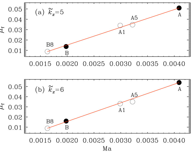
Figure 16: Mode mass of the $f$-mode as a function of ${\rm Ma}$ for $q_{0}=0.1$ and two values of $\widetilde{k}_{x}$ (see Tables 1 and 2). Symbols: values from DNS. Red lines: linear fits with slopes $\sim 16.9$ (a) and $\sim 18.3$ (b).

Figure 17: Properties of the $f$-mode as functions of $\widetilde{k}_{x}$, for $q_{0}=0.1$ (left) and $q_{0}=0.01$ (right). Lines in panels (a) and (b): theoretical estimates from (25). The ‘$+$’ (dotted), ‘$\ast$’ (dashed), ‘$\diamond$’ (dash-dotted) and ‘$\triangle$’ (dash-triple-dotted) in panels (a), (c) and (e) correspond to Runs A1, A3, A4 and A5, respectively. The ‘$\ast$’ (dashed), ‘$\triangle$’ (dash-triple-dotted) and ‘$\square$’ (long-dashed) in panels (b), (d) and (f), respectively, correspond to Runs A3h, A5h and A6h, respectively.

The dependence of $\delta\omega_{\rm fm}^{2}/\omega_{\rm f}^{2}$, $\mu_{\rm f}$ and $\Gamma_{\rm f}$ on the horizontal wavenumber $k_{x}$ in the presence of a magnetic field is shown in Fig. 17 for some of the cases of Table 2, covering both $q_{0}=0.1$ and $q_{0}=0.01$. We recall that, while magnetic fields tend to increase the $f$-mode frequencies (Chandrasekhar, 1961; Roberts, 1981; Miles & Roberts, 1992; Miles et al., 1992), turbulent motions lead to a decrease Murawski (2000a, b); see Sect. 3.2. For weak magnetic fields (Runs A1 and A3 with $v_{{\rm A}x\rm d}/c_{\rm sd}=0.004$ and $0.042$, respectively) we find at large values of $\widetilde{k}_{x}$ considerable frequency decrements compared to the theoretical estimates when $q_{0}=0.1$; see panel (a) of Fig. 17. This is because the magnetic field might here not be sufficient to compensate for the decrease caused by the turbulence. As the strength of the imposed field is increased, $\omega_{{\rm fm}\#}$ also increases and shows reasonably good agreement with the theoretically expected values (23) for Runs A4 and A5. For the hotter corona with $q_{0}=0.01$, numerical findings and theoretical estimates lie even nearly on top of each other, see panel (b). Depending on the strength of the field, the frequencies can be much higher than those of the classical $f$-mode given by Eq. (17). It is interesting to note that, although $v_{\rm A}/c_{\rm s}=0.042$ for both A3 and A3h, the relative frequency shifts are different and smaller for the stronger density jump; compare panels (a) and (b) of Fig. 17. From panels (c)–(f) we note:

1. The mode mass $\mu_{\rm f}$ decreases with $k_{x}$ for all runs. It decreases more rapidly when the density jump is smaller.

2. The distinguishing effect of the imposed field is that the $f$-mode is suppressed beyond some ${k_{x}^{f\rm max}}$, which decreases as we increase $B_{x0}$; compare, e.g., the $k\omega$ diagrams Fig. 3 with Fig. 11 or Fig. 4 with Fig. 14a, for $q_{0}=0.1$ and Fig. 12 with Fig. 13 for $q_{0}=0.01$, respectively.

3. For $q_{0}=0.1$, $\mu_{\rm f}$ does not show any systematic variation with $B_{x0}$ at a fixed $k_{x}$; see panel (c). But for $q_{0}=0.01$, $\mu_{\rm f}$ decreases drastically with increasing $B_{x0}$ for all $k_{x}$; see panel (d).

4. For small $B_{x0}$, $\mu_{\rm f}$ is larger for $q_{0}=0.01$ compared to $q_{0}=0.1$; compare runs A3 and A3h, for both of which $v_{\rm A}/c_{\rm s}=0.042$.

5. For large $B_{x0}$, ${k_{x}^{f\rm max}}$ is smaller for $q_{0}=0.01$ than for $q_{0}=0.1$; compare both panels of Fig. 14. This is the reason why $\mu_{\rm f}$ of run A5 is, for small $\widetilde{k}_{x}$, larger compared to run A5h (both with $v_{\rm A}/c_{\rm s}\approx 0.12$), despite the latter having stronger density contrast.

6. For most runs, the line width $\Gamma_{\rm f}$ increases with $k_{x}$; see panels (e) and (f). Although it does not show any systematic variation with $B_{x0}$ for fixed $k_{x}$ when $q_{0}=0.1$, it increases with $B_{x0}$ at all $k_{x}$ when $q_{0}=0.01$.

To quantify the magnetically produced line shifts, we now consider Runs A1–A6h. It turns out that $\delta\omega_{\rm fm}^{2}/\omega_{\rm f}^{2}$ is approximately proportional to $v_{{\rm A}x\rm d}^{2}/c_{\rm sd}^{2}$, as expected from theory; see Fig. 18 and Eq. (26). We find somewhat larger frequency shifts compared to theory when $q_{0}=0.1$, but better agreement when $q_{0}=0.01$.

To assess the effect of a hotter corona, we plot in Fig. 19 the $k_{x}$ dependencies of $\delta\omega_{\rm fm}^{2}/\omega_{\rm f}^{2}$, $\mu_{\rm f}$ and $\Gamma_{\rm f}$ for models B8 ($q_{0}=0.1$) and B8h ($q_{0}=0.01$). Both runs are for a shallower domain with $L_{z}=\pi$, and have $v_{{\rm A}x\rm d}/c_{\rm sd}\approx 0.3$; see Table 2. Interestingly, the line shifts are slightly reduced for a hotter corona. This behaviour is in agreement with the $q$ dependence of the shifts expected from the theoretical result (25). However, the numerically obtained shifts lie below the theoretical estimates for both runs. As the imposed field $B_{x0}$ is large, the $f$-mode is truncated beyond relatively small values of $\widetilde{k}_{x}$, as may be inferred from Fig. 14. For strong magnetic fields, the Mach numbers are small despite strong forcing; see Table 2. Consequently, the mode mass $\mu_{\rm f}$ is small in both runs, but it drops more rapidly with $k_{x}$ for $q_{0}=0.01$ than for $q_{0}=0.1$; compare panels (c) and (d) of Fig. 17 with panel (b) of Fig. 19 (note the different ranges of the $\widetilde{k}_{x}$ axes). From panel (c) of Fig. 19 we note that the line width $\Gamma_{\rm f}$ increases with $k_{x}$ and is larger for smaller $q_{0}$. All these observations are in qualitative agreement with what we noted before in case of deeper domains; see Fig. 17.

Figure 18: Relative frequency shift $\delta\omega_{\rm fm}^{2}/\omega_{\rm f}^{2}$ as a function of $v_{\rm Ad}^{2}/c_{\rm sd}^{2}$ at $\widetilde{k}_{x}=6$. Lines: estimates from (26), symbols: values from DNS.

Figure 19: Effect of hot corona on mode parameters for horizontal magnetic field. Open/filled circles: Run B8/B8h, both with $v_{\rm A}/c_{\rm s}\approx 0.3$. Dotted/dashed lines in upper panel: theoretical estimates for B8/B8h.

4.3 $g\,$-modes

Remarkably, the $g\,$-modes are strongly suppressed beyond some value $k_{x}^{g\rm max}$, which is found to decrease with increasing $B_{x0}$; compare, e.g., Fig. 3 with Figs. 10 and 11, or Fig. 4 with Fig. 14(a). Varying $q_{0}$ for fixed $B_{x0}$ does not seem to have much effect on the $g\,$-modes; cf. Figs. 14(a) and (b).

Table 3: Summary of simulations with a vertical and oblique magnetic fields in domain $8\pi\times 2\pi$. $\theta$ – inclination of $\bm{B}_{0}$ to $z$ axis.

Run	$\theta$	Grid	$q_{0}$	$q$	$v_{\rm Ad}/c_{\rm sd}$	$v_{\rm Au}/c_{\rm su}$	${\rm Ma}$	${\rm Re}$	${\cal F}$
A2V	$0^{\circ}$	$1024\times 600$	0.1	0.087	0.020	0.020	0.0030	0.536	0.02
A6Vh	$0^{\circ}$	$1024\times 512$	0.01	0.0089	0.117	0.118	0.0011	0.256	0.02	(Fig. 20)
A7Vh	$0^{\circ}$	$1024\times 512$	0.01	0.0096	0.185	0.176	0.0016	0.730	0.04
Obl	$45^{\circ}$	$1024\times 512$	0.01	0.009	0.22	0.22	0.0015	0.35	0.02

5 Vertical and oblique fields

We now turn to cases where the imposed magnetic field is either vertical or points in an oblique direction in the $xz$ plane. There have been earlier attempts to study the interaction of the $f$- and $p\,$-modes with a vertical magnetic field to provide some explanation for the observed absorption of these modes (Cally & Bogdan, 1993; Cally et al., 1994; Cally & Bogdan, 1997). Although the physics of mode absorption is yet to be understood, some explanations in terms of slow mode leakage due to vertical stratification were discussed in these works: it is thought that the partial conversion of the $f$- and $p\,$-modes to slow magnetoacoustic modes, or $s$-modes, takes place whenever they encounter the region of a vertical magnetic field, such as a sunspot. Parchevsky & Kosovichev (2009) numerically investigated the effects of an inclined magnetic field on the excitation and propagation of helioseismically relevant magnetohydrodynamic waves. They found that the $f$-modes are affected by the background magnetic field more than the $p\,$-modes. Such results emphasize the diagnostic role of $f$-modes to reveal the subsurface structure of the magnetic field.

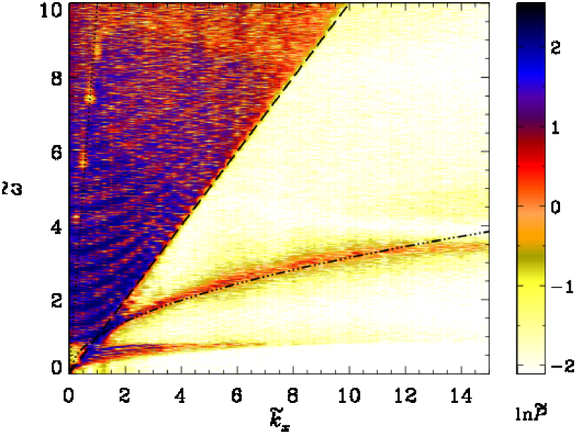
Figure 20: $k\omega$ diagram for Run A6Vh with vertical magnetic field; see Table 3. Dash-triple-dotted: $\omega_{\rm f}$ as defined in Eq. (17). Long dashed: $\omega=c_{\rm sd}k_{x}$.

In Table 3 we summarize the simulations with vertical and oblique magnetic fields. With a vertical magnetic field $(0,0,B_{z0})$, the Alfvén velocities $v_{{\rm A}z\,{\rm d,u}}$ in bulk and corona are defined analogously to Eq. (21).

In Fig. 20 we present the $k\omega$ diagram for Run A6Vh. Remarkably, the frequency shift of the $f$-mode shows a non-monotonic behaviour, unlike those in other $k\omega$ diagrams. Here the frequencies lie above those of the classical $f$-mode given by Eq. (17) (dash-triple-dotted curves in $k\omega$ diagrams) for intermediate wavenumbers, while falling below it for larger wavenumbers. Interestingly, both tendencies have been reported in observational results of Fernandes et al. (1992).

We report on one simulation where the magnetic field points in a direction of $45^{\circ}$ to the $z$-axis. It was performed with $q_{0}=0.01$, and $v_{{\rm A}x\rm d}/c_{\rm sd}=v_{{\rm A}z\rm d}/c_{\rm sd}=0.157$, or $v_{\rm A}/c_{\rm s}=0.22$ for the total field as $v_{\rm A}^{2}=v_{{\rm A}x}^{2}+v_{{\rm A}z}^{2}$.

5.1 $p\,$-modes

In Fig. 21 we plot $\widetilde{P}(\widetilde{\omega})$ at $\widetilde{k}_{x}=4$ for three runs with vertical field (A2V, A6Vh, A7Vh), and for the one with oblique field (Obl); see also Table 3. As before, the dash-dotted (blue) and dashed (red) lines in all panels mark the theoretically expected locations of the $f$- and $p\,$-modes, respectively, all for the non-magnetic case. The group of peaks to the left of the $f$-mode are the $g\,$-modes, whereas those to the right are $p\,$-modes. Note that for higher coronal temperatures, the modes are much more noisy and there appears to be a larger continuum; cf. panels (a) and (d) of Fig. 21. For weaker jumps in the thermodynamic quantities at the interface, we find that $p\,$-mode amplitudes are not much affected by the presence of a weak vertical field; compare e.g. Runs A (non-magnetic) and A2V shown in Figs. 7 and 21, respectively, both having $q_{0}=0.1$. Compared to other cases, we notice a significant reduction in the $p\,$-mode amplitudes in case of the inclined magnetic field, which has $q_{0}=0.01$; see panel (d). The $g\,$- and $f$-modes are also strongly suppressed, which might be caused by the large strength of the magnetic field, leading to the truncation of these modes beyond some wavenumber, $k_{x}\approx 4$.

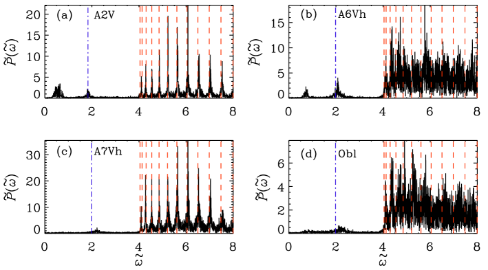
Figure 21: $\widetilde{P}(\widetilde{\omega};\widetilde{k}_{x}=4)$ for a vertical magnetic field for (a) A2V, (b) A6Vh, (c) A7Vh, and (d) for the $45^{\circ}$ inclined magnetic field; see Table 3. Dash-dotted (blue) and dashed (red): theoretically expected $f$- and $p\,$-modes, respectively, all for the non-magnetic case.

5.2 $f$-mode

An analytical dispersion relation of the $f$-mode for vertical magnetic field suitable to our setup is yet to be derived. For quantitative analysis, we compute relative frequency shift $\delta\omega_{\rm fm}^{2}/\omega_{\rm f}^{2}$, mode mass $\mu_{\rm f}$, and dimensionless line width $\Gamma_{\rm f}$ of the $f$-mode for different $k_{x}$, following the procedures described in Sect. 3. In Fig. 22 we show the dependence of the line parameters on $k_{x}$ for Runs A2V (with $q_{0}=0.1$), A6Vh and Run Obl (with $q_{0}=0.01$ for the latter two runs). Some noteworthy observations are:

1. The relative line shift $\delta\omega_{\rm fm}^{2}/\omega_{\rm f}^{2}$ shows a non-monotonic behaviour as a function of $k_{x}$ for sufficiently strong $B_{z0}$, unlike our findings of Sects. 3 and 4 without field or with horizontal field. This holds also for Run A6Vh where we find that $\delta\omega_{\rm fm}^{2}/\omega_{\rm f}^{2}$ reaches a maximum at $\widetilde{k}_{x}=6$, and becomes negative at $\widetilde{k}_{x}=11$.

2. For weak field, $\delta\omega_{\rm fm}^{2}/\omega_{\rm f}^{2}$ is negative and decreases with increasing $k_{x}$ as in non-magnetic cases.

3. For large $B_{z0}$, with or without $B_{x0}$, we find that $\delta\omega_{\rm fm}^{2}/\omega_{\rm f}^{2}$ attains positive values for small $\widetilde{k}_{x}$.

4. For Run Obl, we notice larger positive frequency shifts compared to Run A6Vh. It increases up to about $\widetilde{k}_{x}\approx 6$, beyond which it tends to decrease. Fewer points (filled circles) are shown as the $f$-mode is truncated for larger $\widetilde{k}_{x}$ due to the stronger magnetic field compared to the other runs shown. This truncation effect is also discussed earlier.

5. The mode masses from Runs A2V and A6Vh are comparable, despite the latter having smaller Mach number; see Table 3. This is due to the stronger density jump at the interface in Run A6Vh, and thus consistent with our earlier findings.

6. As the field strength is increased in Run Obl compared with Run A6Vh, $\mu_{\rm f}$ decreases at all $k_{x}$ although both runs have similar Mach numbers.

7. The line width $\Gamma_{\rm f}$ increases with $k_{x}$ and is larger for stronger fields.

8. Compared to the horizontal magnetic field cases, the $f$-mode suppression is not seen for large values of $k_{x}$; cf. Figs. 13 and 20. For vertical magnetic fields, the energy could in principle leave the interface, leading to a reduction of $f$-mode power. This however does not apply in our case owing to the perfect conductor boundary condition.

Figure 22: (a) Relative frequency shift, (b) mode mass and (c) linewidth of the $f$-mode as functions of $\widetilde{k}_{x}$ in the presence of a vertical/oblique magnetic field. Diamonds and open circles: runs A2V and A6Vh, respectively, with vertical field; filled circles: with $45^{\circ}$ inclined magnetic field; all with comparable Mach numbers.

5.3 $g\,$-modes

The $g\,$-modes are found to behave similarly as with horizontal magnetic field and are suppressed beyond some $k_{x}^{g\rm max}$, which decreases with increasing field. This may be inferred from Fig. 21 where the $g\,$-modes are seen to be suppressed at $\widetilde{k}_{x}=4$ with increasing field for both the vertical and the oblique field; compare also with the non-magnetic case in Fig. 7.

6 Conclusions

The prime objective of the present work was to assess the effects of an imposed magnetic field on the $f$-mode, which is known to be particularly sensitive to magnetic fields. One of our motivations is the ultimate application to cases where magnetic flux concentrations are being produced self-consistently through turbulence effects (see, e.g., Brandenburg et al., 2013, 2014). Those investigations have so far mostly been carried out in isothermal domains, which was also the reason for us to choose a piecewise isothermal model, where the jump in temperature and density is needed to allow the $f$-mode to occur.

The resulting setup is in some respects different from that of the Sun and other stars, so one should not be surprised to see features that are not commonly found in the context of helioseismology. One of them is a separatrix within the $p\,$-modes as a result of the hot corona, which we associate with the $a$-mode of Hindman & Zweibel (1994).

Regarding the $f$-mode, there are various aspects that can be studied even in the absence of a magnetic field. Particularly important is the linearly $k_{x}$-dependent decrease of $\omega_{\rm f}$. The $f$-mode mass increases with the intensity of the forcing and hence with the Mach number. Interestingly, this is also a feature that carries over to the magnetic case where an increase in the magnetic field leads to a decrease in the resulting Mach number and thereby to a decrease in the mode mass in much the same way as in the non-magnetic case. Magnetic fields also lead to a truncated $f$-mode branch above a certain value of $k_{x}$.

One of the most important findings is the systematic increase of the $f$-mode frequencies ${\omega_{{\rm fm}\#}}$ observed in DNS with the horizontal magnetic field. It follows essentially the theoretical prediction and, contrary to the non-magnetic cases, shows an increase with $k_{x}$ such that the relative frequency shift is approximately proportional to $v_{\rm A}^{2}/c_{\rm s}^{2}$. This is best measured when $k_{x}L_{0}=5$–$7$, i.e., $k_{x}H_{p}=3$–$4$, and with a solar radius of $700\,{\rm Mm}$, being 2000 times larger than $H_{p}\approx 300\,{\rm km}$, the corresponding spherical harmonic degree would be 6000–8000. In this range, the relative frequency shift is $\delta\omega_{\rm fm}^{2}/\omega_{\rm f}^{2}\approx 0.1$ when $v_{\rm A}/c_{\rm s}\approx 0.1$. Since $\delta\omega_{\rm fm}^{2}/\omega_{\rm f}^{2}\approx 2\delta\omega_{\rm fm}/\omega_{\rm f}$, the increase of the $f$-mode frequencies is about 5%. The observed $f$-mode frequency increase during solar maximum is about $1\,\mu{\rm Hz}$ at a moderate spherical degree of 200 (Dziembowski & Goode, 2005). This corresponds to a relative shift of about 0.06%, but this value should of course increase with the spherical degree.

We note that in our case, the magnetic field is the same above and below the interface. Furthermore, $\rho c_{\rm s}^{2}$ is also the same above and below the interface, and so is therefore also $v_{\rm A}^{2}/c_{\rm s}^{2}$. One of the goals of future studies will be to determine how our results would change if the magnetic field existed only below the interface.

Interestingly, for vertical and oblique magnetic fields, the $k_{x}$-dependence of ${\omega_{{\rm fm}\#}}$ becomes non-monotonic in such a way that for small values of $k_{x}$, ${\omega_{{\rm fm}\#}}$ first increases with $k_{x}$ and then decreases and becomes less than the theoretical value in the absence of a magnetic field, although it stays above the value obtained without magnetic field, whose reduction is believed to be due to turbulence effects (Mȩdrek et al., 1999; Mole et al., 2008).

We confirm the numerical results of Parchevsky & Kosovichev (2009) that $p\,$-modes are less affected by a background magnetic field than the $f$-mode. Relative to the non-magnetic case, no significant frequency shifts of $p\,$-modes are seen in a weakly magnetized environment. For a larger density contrast at the interface, with the rest of the parameters being same, the mode amplitudes and line widths increase, but the data look more noisy and the frequency shifts, which can be of either sign (Hindman & Zweibel, 1994), may not be primarily due to the magnetic field.

The present investigations allow us now to proceed to more complicated systems where the magnetic field shows local flux concentrations which might ultimately resemble active regions and sunspots. As an intermediate step, one could also impose a non-uniform magnetic field with a sinusoidal variation in the horizontal direction. This will be the focus of a future investigation.

References

- Antia (1998) Antia, H. M. 1998, A&A, 330, 336
- Antia (2003) Antia, H. M. 2003, ApJ, 590, 567
- Antia et al. (2000) Antia, H. M., Basu, S., Pintar, J., & Pohl, B. 2000, Solar Phys., 192, 459
- Birch et al. (2013) Birch, A. C., Braun, D. C., Leka, K. D., Barnes, G., & Javornik, B. 2013, ApJ, 762, 131
- Brandenburg (2001) Brandenburg, A. 2001, ApJ, 550, 824
- Brandenburg (2005) Brandenburg, A. 2005, ApJ, 625, 539
- Brandenburg et al. (2014) Brandenburg, A., Gressel, O., Jabbari, S., Kleeorin, N., & Rogachevskii, I. 2014, A&A, 562, A53
- Brandenburg et al. (2013) Brandenburg, A., Kleeorin, N., & Rogachevskii, I. 2013, ApJ, 776, L23
- Braun (2012) Braun, D. C. 2012, Science, 336, 296
- Caligari et al. (1995) Caligari, P., Moreno-Insertis, F., & Schüssler, M. 1995, ApJ, 441, 886
- Cally (2006) Cally, P. S. 2006, Roy. Soc. Lond. Trans. Ser. A, 364, 333
- Cally & Bogdan (1993) Cally, P. S., & Bogdan, T. J. 1993, ApJ, 402, 721
- Cally & Bogdan (1997) Cally, P. S., & Bogdan, T. J. 1997, ApJ, 486, L67
- Cally et al. (1994) Cally, P. S., Bogdan, T. J., & Zweibel, E. G. 1994, ApJ, 437, 505
- Campbell & Roberts (1989) Campbell, W. R., & Roberts, B. 1989, ApJ, 338, 538
- Campos (2011) Campos, L. M. B. C., 2011, MNRAS, 410, 717
- Chandrasekhar (1961) Chandrasekhar, S. 1961, Hydrodynamic and Hydromagnetic Stability (Dover Publications, New York)
- Christensen-Dalsgaard (2003) Christensen-Dalsgaard, J., 2003, Lecture notes on stellar oscillations, 5th edition
- Daiffallah et al. (2011) Daiffallah, K., Abdelatif, T., Bendib, A., Cameron, R., & Gizon, L. 2011, Solar Phys., 268, 309
- Dungey & Loughhead (1954) Dungey, J. W., Loughhead, R. E. 1954, Austr. J. Phys., 7, 5
- Duvall (1982) Duvall, T. L., Jr. 1982, Nature, 300, 242
- Duvall et al. (1998) Duvall, T. L., Jr., Kosovichev, A. G., & Murawski, K. 1998, ApJ, 505, L55
- Dzhalilov et al. (2000) Dzhalilov, N. S., Staude, J., & Arlt, K. 2000, A&A, 361, 1127
- Dziembowski & Goode (2005) Dziembowski, W. A., & Goode, P. R. 2005, ApJ, 625, 548
- Dziembowski et al. (2001) Dziembowski, W. A., Goode, P. R., & Schou, J. 2001, ApJ, 553, 897
- Evans & Roberts (1990) Evans, David J., & Roberts, B. 1990, ApJ, 356, 704
- Felipe et al. (2012) Felipe, T., Braun, D., Crouch, A., & Birch, A. 2012, ApJ, 757, 148
- Felipe et al. (2013) Felipe, T., Crouch, A., & Birch, A. 2013, ApJ, 775, 74
- Fernandes et al. (1992) Fernandes, D. N., Scherrer, P. H., Tarbell, T. D., & Title, A. M. 1992, ApJ, 392, 736
- Georgobiani et al. (2007) Georgobiani, D., Zhao, J., Kosovichev, A. G., Benson, D., Stein, R. F., & Nordlund, Å. 2007, ApJ, 657, 1157
- Gerwin (1967) Gerwin, R., 1967, Phys. Fluids, 10, 2164
- Ghosh et al. (1995) Ghosh, P., Antia, H. M., & Chitre, S. M. 1995, ApJ, 451, 851
- Gizon et al. (2010) Gizon, L., Birch, A. C., & Spruit, H. C. 2010, ARA&A, 48, 289
- Goldreich & Kumar (1988) Goldreich, P., & Kumar, P. 1988, ApJ, 326, 462
- Goldreich & Kumar (1990) Goldreich, P., & Kumar, P. 1990, ApJ, 363, 694
- Gough (1987) Gough, D. O. 1987, in Astrophysical fluid dynamics, ed. J.-P. Zahn & J. Zinn-Justin (North-Holland, Amsterdam), 399
- Hanasoge et al. (2008) Hanasoge, S. M., Birch, A. C., Bogdan, T. J., & Gizon, L. 2008, ApJ, 680, 774
- Hanasoge et al. (2012) Hanasoge, S. M., Duvall, T. L., & Sreenivasan, K. R. 2012, Proc. Nat. Acad. Sci., 109, 11928
- Hindman & Zweibel (1994) Hindman, B. W., & Zweibel, E. G. 1994, ApJ, 436, 929
- Ilonidis et al. (2011) Ilonidis, S., Zhao, J., & Kosovichev, A. 2011, Science, 333, 993
- Kitiashvili et al. (2011) Kitiashvili, I. N., Kosovichev, A. G., Mansour, N. N., & Wray, A. A. 2011, Solar Phys., 268, 283
- Kruskal & Schwarzschild (1954) Kruskal, M., & Schwarzschild, M., 1954, Proc. Roy. Soc. Lond. Ser. A, Math. Phys. Sci., 223, 348
- Lefebvre & Kosovichev (2005) Lefebvre, S., & Kosovichev, A. G. 2005, ApJ, 633, L149
- Markwardt (2009) Markwardt, C. B., 2009, Astron. Data Anal. Softw. Syst. XVIII, 411, 251, http://purl.com/net/mpfit
- Mȩdrek et al. (1999) Mȩdrek, M., Murawski, K., & Roberts, B. 1999, A&A, 349, 312
- Miles & Roberts (1989) Miles, A. J., & Roberts, B. 1989, Solar Phys., 119, 257
- Miles & Roberts (1992) Miles, A. J., & Roberts, B. 1992, Solar Phys., 141, 205
- Miles et al. (1992) Miles, A. J., Allen, H. R., & Roberts, B. 1992, Solar Phys., 141, 235
- Mole et al. (2008) Mole, N., Kerekes, A., & Erdélyi, R. 2008, Solar Phys., 251, 453
- Murawski (2000a) Murawski, K. 2000a, ApJ, 537, 495
- Murawski (2000b) Murawski, K. 2000b, A&A, 360, 707
- Murawski & Roberts (1993a) Murawski, K. and Roberts, B. 1993a, A&A, 272, 595
- Murawski & Roberts (1993b) Murawski, K. and Roberts, B. 1993b, A&A, 272, 601
- Nye & Thomas (1976) Nye, A. H., & Thomas, J. H. 1976, ApJ, 204, 573
- Parchevsky & Kosovichev (2009) Parchevsky, K. V., & Kosovichev, A. G. 2009, ApJ, 694, 573
- Roberts (1981) Roberts, B. 1981, Solar Phys., 69, 27
- Rosenthal & Christensen-Dalsgaard (1995) Rosenthal, C. S., & Christensen-Dalsgaard, J. 1995, MNRAS, 276, 1003
- Rosenthal & Gough (1994) Rosenthal, C. S., & Gough, D. O. 1994, ApJ, 423, 488
- Schou et al. (1997) Schou, J., Kosovichev, A. G., Goode, P. R., & Dziembowski, W. A. 1997, ApJ, 489, L197
- Schunker & Cally (2006) Schunker, H., & Cally, P. S. 2006, MNRAS, 372, 551
- Singh et al. (2014) Singh, N. K., Brandenburg, A., & Rheinhardt, M. 2014, ApJ, 795, L8
- Stein (1967) Stein, R. F. 1967, Solar Phys., 2, 385
- Stein & Leibacher (1974) Stein, R. F., & Leibacher, J. 1974, ARA&A, 12, 407
- Stein & Nordlund (2012) Stein, R. F., & Nordlund, Å. 2012, ApJ, 753, L13
- Thomas (1983) Thomas, J. H. 1983, Ann. Rev. Fluid Mech., 15, 321
- Wagner & Schmitz (2007) Wagner, M., & Schmitz, F. 2007, A&A, 472, 897