Exit from accelerated regimes by symmetry breaking in a universe filled with fermionic and bosonic sources

Abstract

In this work we investigate a universe filled with a fermionic field and a complex scalar field, exchanging energy through a Yukawa potential; the model encodes a symmetry breaking mechanism (on the bosonic sector). In a first case, when the mechanism is not included, the cosmological model furnishes a pure accelerated regime. In a second case, when including the symmetry breaking mechanism, we verify that the fermion and one of the bosons, of Higgs type, become massive, while the other boson is massless. Besides, the mechanism shows to be responsible for a transition from an accelerated to a decelerated regime, which certifies the importance, in cosmological terms, of its role. After symmetry breaking, the total pressure of the fields change its sign from negative to positive corresponding to the accelerated-decelerated transition. For large times the universe becomes a dust (pressureless) dominated Universe.

1 Introduction

Cosmological models that include fermionic sources are candidates for explaining regimes of positive acceleration, and they have been studied recently in the works [1, 2, 3, 4, 5, 6, 7, 8, 9, 10]. Following in that direction one possibility is, in particular, to consider these fermionic fields as gravitational sources for early universes. These cases have been investigated by using several approaches, with results including exact solutions, anisotropy-to-isotropy scenarios and self-interacting potentials (see for example [1, 2, 3, 4, 11, 6, 7, 8, 9, 10]).

An interesting question would be to investigate if it is possible to implement a symmetry breaking mechanism [12, 13, 14, 15], including fermionic sources in a cosmological context. Furthermore, it would be important to verify if this mechanism permit the entrance into a decelerated period dominated (for instance) by a bosonic constituent. Taking these ideas into account, in this work we propose the description of a universe leaving an initial accelerated period, including two constituents: a massless Dirac fermion and a complex scalar boson (also massless), interacting, as in our previous effort[16], through a Yukawa potential. The fundamental point here is that the model lagrangian encodes, besides the diffeomorphism local invariance[17], typical of gravitational theories, a global symmetry controlled by the group structure U(1) [12, 13, 14, 15]; of which the complex scalar field, mentioned above, would be a representation. Another fundamental fact is that the symmetry breaking mechanism [12, 13, 14, 15] associated to the U(1) invariance would be responsible for the generation of mass in this universe, and the symmetry breaking condition would be represented by this system reaching the so-called false-vacuum state [18, 19, 20]. As expected, the false vacuum is in fact a continuum of vacua. The permanent universe expansion implies into the system choosing one of these vacua, and the U(1) symmetry is therefore broken [12, 13, 14, 15]. As far as this state must be related to observables the symmetry charge operator acting on the vacuum state cannot give a different from zero result [12, 13, 14, 15]. So, speaking in terms of the lagrangian formalism, the field variables must be redefined in order to have a well-structured lowest-energy state [12, 13, 14, 15]. This new lagrangian density would be the starting point for the dynamics after the symmetry breaking, and, under proper conditions, would describe the universe entering into a permanently decelerated period.

Therefore, in few words, we want to focus on the symmetry breaking mechanism and want to investigate what kind of role this mechanism precisely plays in an initially accelerating universe. First, it is shown that without the symmetry breaking mechanism the cosmological model furnishes a pure accelerated regime. Second, when the symmetry is broken the fermion and one of the bosons become massive, while the other boson remains massless. The massive boson is identified as a Higgs-type boson, and the massless as a Goldstone boson [12, 13, 14, 15]. Then, the symmetry breaking mechanism would be answering for the accelerated-decelerated transition.

The work is structured as follows: in Section II we present the action which includes a massless and non-self-interacting Dirac field and a massless complex scalar field with a self-interacting potential. These two fields interacts through a Yukawa-type potential. The analysis of universe evolution without the symmetry breaking mechanism is given in Section III, while in Section IV we introduce the Lagrangian and the corresponding field equations after the symmetry breaking. In Section V we show a numerical solution of the field equations with the accelerated-decelerated transition and the evolution of the total pressure of the sources of the gravitational field. We state the main conclusion of the work in Section VI. The metric signature used is $(+,-,-,-)$ and units have been chosen so that $8\pi G=c=\hbar=1$.

2 The action

We are interested in investigating a cosmological model described by a scalar and a Dirac field. The scalar field $\phi$ is complex, massless with a self-interacting potential. The Dirac field $\psi$ is also massless and interacts with the complex scalar field through a Yukawa potential. The action is invariant with respect to a global symmetry controlled by the group structure U(1) and reads

$$S=\int\sqrt{-g}\,d^{4}x\bigg{[}\frac{1}{2}R+\frac{1}{2}\partial_{\mu}\phi^{*}\partial^{\mu}\phi-V(\phi^{*}\phi)+Y(\overline{\psi}\psi,\phi^{*}\phi)$$

$$+\frac{i}{2}\left(\overline{\psi}\Gamma^{\mu}D_{\mu}\psi-D_{\mu}\overline{\psi}\Gamma^{\mu}\psi\right)\bigg{]}.$$ (1)

Here $R$ denotes the scalar curvature, while $\psi$ and $\overline{\psi}=\psi^{\dagger}\gamma^{0}$ are the spinor field and its adjoint, respectively. According to the general covariance principle, the $4\times 4$ Dirac-Pauli matrices

$$\gamma^{0}=\left(\begin{array}[]{cc}1&0\\ 0&-1\\ \end{array}\right),\qquad\gamma^{i}=\left(\begin{array}[]{cc}0&\sigma^{i}\\ -\sigma^{i}&0\\ \end{array}\right),$$ (6)

are replaced by their generalized versions $\Gamma^{\mu}=e^{\mu}_{a}\gamma^{a}$, where $\sigma^{i}$ are the $2\times 2$ Pauli matrices and $e^{\mu}_{a}$ the tetrad fields. Furthermore, the $\Gamma^{\mu}$ matrices satisfy the generalized Clifford algebra $\{\Gamma^{\mu},\Gamma^{\nu}\}=2g^{\mu\nu}$. The covariant derivatives in (1) read

$$D_{\mu}\psi=\partial_{\mu}\psi-\Omega_{\mu}\psi,\qquad D_{\mu}\overline{\psi}=\partial_{\mu}\overline{\psi}+\overline{\psi}\Omega_{\mu},$$ (7)

where $\Omega_{\mu}$ is the spin connection

$$\Omega_{\mu}=-\frac{1}{4}g_{\rho\sigma}[\Gamma^{\rho}_{\mu\delta}-e_{b}^{\rho}(\partial_{\mu}e_{\delta}^{b})]\Gamma^{\delta}\Gamma^{\sigma},$$ (8)

and $\Gamma^{\nu}_{\sigma\lambda}$ the Christoffel symbols.

The interaction between the fields is given by the Yukawa potential $Y(\overline{\psi}\psi,\phi^{*}\phi)=-\lambda\overline{\psi}\psi\phi^{*}\phi$ with $\lambda$ denoting a constant. Furthemore, the self-interacting potential of the complex scalar field reads

$$V(\phi^{*}\phi)=-\frac{1}{2}\mu^{2}\phi^{*}\phi+\frac{1}{4}\xi^{2}(\phi^{*}\phi)^{2},$$ (9)

where $\mu$ and $\xi$ are constants.

3 Before symmetry breaking

The determination of the field equations are obtained from the variation of the action (1) with respect the fields.

From the variation of (1) with respect to the scalar fields $\phi$ and $\phi^{*}$ we get the Klein-Gordon equations

$$\nabla_{\mu}\nabla^{\mu}\phi-\mu^{2}\phi+\xi^{2}(\phi\phi^{*})\phi+2\lambda\overline{\psi}\psi\phi=0,$$ (10)

$$\nabla_{\mu}\nabla^{\mu}\phi^{*}-\mu^{2}\phi^{*}+\xi^{2}(\phi\phi^{*})\phi^{*}+2\lambda\overline{\psi}\psi\phi^{*}=0.$$ (11)

Dirac’s equations are obtained from the variation of the action wit respect to $\overline{\psi}$ and $\psi$, yielding,

$$i\Gamma^{\mu}D_{\mu}\psi-\lambda\phi\phi^{*}\psi=0,\qquad iD_{\mu}\overline{\psi}\Gamma^{\mu}+\lambda\overline{\psi}\phi\phi^{*}=0.$$ (12)

Furthermore, the left multiplication of the first equation by $\overline{\psi}$ summed with the right multiplication of the second one by $\psi$ leads to

$$\overline{\psi}\Gamma^{\mu}D_{\mu}\psi+D_{\mu}\overline{\psi}\Gamma^{\mu}\psi=0.$$ (13)

The variation of (1) with respect to the tetrad lead to Einstein’s field equations

$$R_{\mu\nu}-\frac{1}{2}g_{\mu\nu}R=-T_{\mu\nu},$$ (14)

where the energy-momentum tensor of the sources of the gravitational field reads

$$T^{\mu\nu}=\frac{i}{4}\left[\overline{\psi}\Gamma^{\mu}D^{\nu}\psi+\overline{\psi}\Gamma^{\nu}D^{\mu}\psi-D^{\nu}\overline{\psi}\Gamma^{\mu}\psi-D^{\mu}\overline{\psi}\Gamma^{\nu}\psi\right]+\frac{1}{2}\left[\partial^{\mu}\phi^{*}\partial^{\nu}\phi\right.$$

$$\left.+\partial^{\nu}\phi^{*}\partial^{\mu}\phi\right]-g^{\mu\nu}\bigg{[}\frac{1}{2}\partial^{\rho}\phi^{*}\partial_{\rho}\phi-V(\phi^{*}\phi)+Y(\overline{\psi}\psi,\phi^{*}\phi)$$

$$+\frac{i}{2}\left(\overline{\psi}\Gamma^{\lambda}D_{\lambda}\psi-D_{\lambda}\overline{\psi}\Gamma^{\lambda}\psi\right)\bigg{]}.$$ (15)

Let us consider the case of a homogeneous and isotropic Universe spatially flat, described by the Friedmann-Robertson-Walker (FRW) metric

$$ds^{2}=dt^{2}-a(t)^{2}(dx^{2}+dy^{2}+dz^{2})$$ (16)

where $a(t)$ denotes the cosmological scale factor. In this case the Dirac-Pauli matrices and spin connection become

$$\Gamma^{0}=\gamma^{0},\qquad\Gamma^{i}=\frac{1}{a(t)}\gamma^{i},\qquad\Omega_{0}=0,\qquad\Omega_{i}=\frac{1}{2}\dot{a}(t)\gamma^{i}\gamma^{0},$$ (17)

with the dot denoting time derivative.

For the FRW metric the acceleration equation that follows from Einstein’s field equations (14) reads

$$\frac{\ddot{a}}{a}=-\frac{1}{6}\left(\rho+3p\right),$$ (18)

where $\rho$ is the the energy density and $p$ the pressure $p$. Their expressions can be obtained from the energy-momentum tensor (15) and are given by

$$\rho=\frac{1}{2}\dot{\phi}^{*}\dot{\phi}+V(\phi^{*}\phi)-Y(\overline{\psi}\psi,\phi^{*}\phi),$$ (19)

$$p=\frac{1}{2}\dot{\phi}^{*}\dot{\phi}-V(\phi^{*}\phi).$$ (20)

When the kinetic term is much smaller than the potential one $\dot{\phi}^{*}\dot{\phi}/2\ll V(\phi^{*}\phi)$, the following relationship between the pressure and energy density can be established:

$$p=-\rho-Y(\overline{\psi}\psi,\phi^{*}\phi),$$ (21)

Let us analyze the sign of the acceleration equation (18) when the condition $\dot{\phi}^{*}\dot{\phi}/2\ll V(\phi^{*}\phi)$ is satisfied. In this case

$$\rho+3p=-2V(\phi^{*}\phi)-Y(\overline{\psi}\psi,\phi^{*}\phi).$$ (22)

According to the weak energy condition (see e.g. [21]) $\rho+p\geq 0$ and $\rho\geq 0$, so that we have

$$Y(\overline{\psi}\psi,\phi^{*}\phi)=-\lambda\overline{\psi}\psi\phi^{*}\phi\leq 0,\qquad V(\phi^{*}\phi)\geq Y(\overline{\psi}\psi,\phi^{*}\phi),$$ (23)

respectively. From the first equation above we conclude that $\lambda>0$, provided that $\overline{\psi}\psi\phi^{*}\phi$ is a positive real number. The second one implies that $\rho+3p<0$ which together with (18) implies that $\ddot{a}>0$, i.e., we are in the presence of an accelerated regime .

Hence under the condition $\dot{\phi}^{*}\dot{\phi}/2\ll V(\phi^{*}\phi)$ we have a pure accelerated regime and we need a mechanism to generate masses in order to bring the Universe to a decelerated regime. In other words, the cosmological solutions of the field equations permit an eternal expansion with the energy density of the field constituents reaching a critical value at some point in the evolution. This critical values are related to the vacuum state of the scalar field and this promotes breaking of the U(1) symmetry. As far as this state must be related to an observable the field variables must be redefined in order to have a well-structured lower-energy state.

Through the symmetry breaking process the fermion and the new boson acquire masses, as expected (see e.g. [12, 13, 14, 15]). This is to be considered the starting point of a new period in the evolution of the Universe, as far as the symmetry breaking permits the exit from an accelerated period and the entrance on a decelerated era, which is a characteristic of a matter dominated universe. It is important to reinforce here that the original Lagrangian does not show a decelerated period among its solutions. In fact, the end of accelerated period is possible only because of the symmetry breaking process, translated by the use of new field dynamics controlled by a new Lagrangian which will be analyzed in the next section.

4 After symmetry breaking

A fundamental point here is that the Lagrangian encodes, besides the local diffeomorphism invariance, a global symmetry controlled by the group structure U(1). This property will be crucial for our purposes, since a symmetry breaking mechanism associated to the U(1) invariance would be responsible for the generation of mass in this universe.

For the action (1) we shall use the Higgs-Goldstone mechanism for mass generation of the fermions and bosons fields, from the choice of a stable potential minimum during its decay, breaking the global symmetry of the system. The fields acquire masses with the breaking symmetry mechanism, that is, we expand the fields around the potential minimum. The action (1) is invariant with respect to the transformations of the global group U(1), characterized by $\phi\longrightarrow\phi e^{i\chi}$, where $\chi$ is global parameter that does not depend on the local space-time.

The minimum of the field does not occur for $\phi=0$ and the symmetry breaking condition is represented by the system reaching the so-called false-vacuum state by imposing that ${dV}/{d\phi}=0$. This condition implies that the components of the complex scalar field are given by

$$\phi_{1(0)}=\frac{\mu}{\xi}\cos\theta,\qquad\phi_{2(0)}=\frac{\mu}{\xi}\sin\theta.$$ (24)

Furthermore, as vacuum condition, we impose

$$\langle 0\mid\phi\mid 0\rangle=\frac{\mu}{\xi}e^{i\theta},$$ (25)

where $\theta$ is the angle that defines a particular minimum. As expected, the false vacuum is in fact a continuum of vacua, labelled by the $\theta$ parameter of expression (25). The permanent universe expansion implies into the system choosing one of these vacua, and the U(1) symmetry is therefore broken. We stress that $\phi\mid 0\rangle$ is not orthogonal to the vacuum state, making difficult to give an interpretation in terms of particles due to the fact that in this case the state $\phi\mid 0\rangle$ would had a non-zero number of particles, and besides that it is not orthogonal to the vacuum state. As far as this state must be related to an observable the field variables must be redefined in order to have a well-structured lowest-energy state. The new fields are defined by the following equations:

$$\Phi=\phi-\langle 0\mid\phi\mid 0\rangle,$$ (26)

with $\Phi=\varphi+i\eta$ where $\varphi$ and $\eta$ are real scalar fields. With these new variables we recover the correct particle interpretation because of the condition $\langle 0\mid\Phi\mid 0\rangle=0,$. Expanding the action (1) in terms of the new fields

$$\phi=\varphi+i\eta+\frac{\mu}{\xi}e^{i\theta},\qquad\phi^{*}=\varphi-i\eta+\frac{\mu}{\xi}e^{-i\theta}$$ (27)

we obtain a new action with U(1) symmetry broken. This new action describes a distinct cosmological model of the previous section, since apart from the massive fields we have new types of interaction vertices, as we shall show in the sequence.

The modifications which are introduced in the action (1) are:

$$\partial_{\mu}\phi^{*}\partial^{\mu}\phi=\frac{1}{2}\partial_{\mu}\varphi\partial^{\mu}\varphi+\frac{1}{2}\partial_{\mu}\eta\partial^{\mu}\eta,$$ (28)

$$V(\phi^{*}\phi)=\mu\xi\eta^{3}\sin\theta+\mu\xi\eta\varphi^{2}\sin\theta+2\mu^{2}\eta\varphi\cos\theta\sin\theta+\mu\xi\varphi\eta^{2}\cos\theta$$

$$+\mu\xi\varphi^{3}\cos\theta+\mu^{2}\varphi^{2}\cos^{2}\theta-\frac{\mu^{4}}{4\xi^{2}}+\frac{1}{2}\xi^{2}\eta^{2}\varphi^{2}+\mu^{2}\eta^{2}\sin^{2}\theta+\frac{1}{4}\xi^{2}\left(\eta^{4}+\varphi^{4}\right),$$ (29)

$$Y(\overline{\psi}\psi,\phi^{*}\phi)=-\lambda\overline{\psi}\psi\left(\varphi^{2}+\eta^{2}+2\varphi\frac{\mu}{\xi}\cos\theta+2\eta\frac{\mu}{\xi}\sin\theta+\frac{\mu^{2}}{\xi^{2}}\right).$$ (30)

Given the symmetry of the potential, the choice of the angle θ which leads to the new minimum of the potential should be immaterial. On the other hand, for a general $\theta$ the Lagrangian above apparently contains two massive bosonic fields, $\phi$ and $\eta$, thus, violating Goldstone theorem (see e.g. [12, 13, 14, 15]). It should be noted, however, that any interacting terms $\phi\eta$ renders the mass matrix off-diagonal and the masses of the free bosonic fields can no longer be identified. Only when the mass matrix is diagonal ($\theta=\pi/2$ or $\theta=3\pi/2$) can the Lagrangian contain the physical fields. Since the vacuum state is degenerated after the symmetry breaking the system choose one of these states. Following the usual choice of the standard model we fix the vacuum state by considering $\theta=\pi/2$.

With the above choice the action (1) becomes

$$S=\int\sqrt{-g}\,d^{4}x\bigg{[}\frac{1}{2}R+\frac{1}{2}\partial_{\mu}\eta\partial^{\mu}\eta-m_{b}\eta^{2}+\frac{i}{2}\left(\overline{\psi}\Gamma^{\mu}D_{\mu}\psi-D_{\mu}\overline{\psi}\Gamma^{\mu}\psi\right)$$

$$+\frac{1}{2}\partial_{\mu}\varphi\partial^{\mu}\varphi-m_{f}\overline{\psi}\psi-\widetilde{V}(\eta,\varphi)+\widetilde{Y}(\overline{\psi}\psi,\eta,\varphi)\bigg{]},$$ (31)

where have introduced the modified potentials

$$\widetilde{V}(\eta,\varphi)=\left(\eta^{2}+\varphi^{2}\right)\left[\mu\xi\eta+\frac{1}{4}\xi^{2}\left(\eta^{2}+\varphi^{2}\right)\right]-\frac{\mu^{4}}{4\xi^{2}},$$ (32)

$$\widetilde{Y}(\overline{\psi}\psi,\eta,\varphi)=-\lambda\overline{\psi}\psi\left(\varphi^{2}+\eta^{2}+2\frac{\mu}{\xi}\eta\right).$$ (33)

From (31) we infer that after symmetry breaking the Dirac field becomes massive due to its coupling with the scalar field through the Yukawa potential. Furthermore, the boson field $\eta$ also becomes massive. The masses of the fermion and boson fields are given by $m_{f}=\lambda{\mu^{2}}/{\xi^{2}}$ and $m_{b}=\mu$, respectively. After the symmetry breaking process we have a massless scalar field $\varphi$, whose quanta are known as Goldstone boson. Certainly these results agree with Goldstone theorem, which states that a continuous symmetry breaking implies in the existence of a boson with vanishing mass, the so-called Goldstone boson. In the case of symmetry breaking in local groups in gauge theories, the same theorem is valid, however the field associated with the Goldstone boson can be absorbed by a gauge vectorial field by the choice of an adequate gauge. In this manner the vectorial field acquires mass and gains one longitudinal degree of freedom. The massive boson cannot be eliminated by gauge choices and in the standard model of interactions it is know as Higgs boson and the mechanism associated with this process as Higgs mechanism.

It is worth to call attention to the fact that with the identification of the mass of the Dirac field, the modified Yukawa potential (33) is a real interaction potential, since it is written in terms of products of the invariant of the spinors $\overline{\psi}\psi$ with the scalar fields $\eta$ and $\varphi$.

5 Solution of the field equations

In order to determine the cosmological solutions we have to solve the following system of coupled equations, which are written according to the FRW metric (16):

$$\ddot{\eta}+3\frac{\dot{a}}{a}\dot{\eta}+\mu\xi(3\eta^{2}+\varphi^{2})+\xi^{2}\eta(\varphi^{2}+\eta^{2})+2\mu^{2}\eta-2\overline{\psi}\psi\left(\eta+\frac{\mu}{\xi}\right)=0,$$ (34)

$$\ddot{\varphi}+3\frac{\dot{a}}{a}\dot{\varphi}+2\mu\xi\eta\varphi+\xi^{2}\varphi(\eta^{2}+\varphi^{2})-2\overline{\psi}\psi\varphi=0,$$ (35)

$$\dot{\overline{\psi}}\psi+\overline{\psi}\dot{\psi}+3\frac{\dot{a}}{a}\overline{\psi}\psi=0,$$ (36)

$$\frac{\ddot{a}}{a}=-\frac{1}{6}\left(\rho+3p\right),$$ (37)

where the energy density $\rho$ and the pressure $p$ are given by

$$\rho=\frac{1}{2}\dot{\eta}^{2}+\frac{1}{2}\dot{\varphi}^{2}-\lambda\overline{\psi}\psi\left(\varphi^{2}+\eta^{2}+\frac{2\mu}{\xi}\eta+\frac{\mu^{2}}{\xi^{2}}\right)+\mu\xi\eta(\varphi^{2}+\eta^{2})$$

$$+\mu^{2}\eta^{2}+\frac{1}{4}\xi^{2}\eta^{2}(\varphi^{2}+\eta^{2})^{2}-\frac{\mu^{4}}{4\xi^{2}},$$ (38)

$$p=\frac{1}{2}\dot{\eta}^{2}+\frac{1}{2}\dot{\varphi}^{2}-\mu\xi\eta(\varphi^{2}+\eta^{2})-\frac{1}{4}\xi^{2}\eta^{2}(\varphi^{2}+\eta^{2})^{2}-\mu^{2}\eta^{2}+\frac{\mu^{4}}{4\xi^{2}}.$$ (39)

Equations (34), (35) and (36) follow from (10), (11) and (13), respectively.

From the coupled system of equations (34) – (37) one may see that an algebraic solution of this system is very difficult. The only equation that can be integrated is (36), whose solution is $\overline{\psi}\psi=C/a^{3}$, where $C$ is a constant of integration. Even the numerical solution is very complicated, since apart from the four constants $\lambda,\mu,\xi,C$ we need six initial conditions, namely, $(a(0),\dot{a}(0))$, $(\eta(0),\dot{\eta}(0))$ and $(\varphi(0),\dot{\varphi}(0))$. One of constants can be eliminated, because only the product $C\lambda$ appears in the equations. Moreover, we need only to specify the initial condition for $a(0)$, since the initial condition for $\dot{a}(0)$ can be obtained from the Friedmann equation

$$\dot{a}(0)=a(0)\sqrt{\frac{\rho(0)}{3}}.$$ (40)

In the figures 1 and 2 the parameters chosen were $C\lambda=1.5\times 10^{-5}$, $\mu=10^{-6}$, $\xi=0.17$ and the initial conditions $a(0)=1$, $\varphi(0)=0.25$, $\dot{\varphi}(0)=9\times 10^{-5}$, $\eta(0)=0.993$ and $\dot{\eta}(0)=3.4\times 10^{-4}$.

         

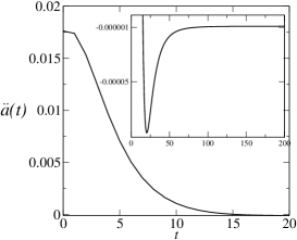
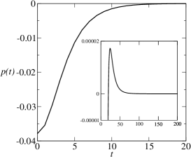
Figure 1: Left frame: Acceleration $\ddot{a}$ versus time $t$; right frame: pressure $p$ versus time $t$.

We observe from the left frame of Fig.1 that a strong accelerated regime for $0\leq t\approx 20$ is followed by a weak decelerated regime for $t>20$ that extends for a long period of time (see the inset in this figure). The transition from an accelerated to a decelerated regime is a consequence of the symmetry breaking and the generation of two massive terms, a fermion and a boson. The right frame of Fig. 1 confirms also that this transition is connected to the fact that a large negative pressure that goes to zero for $0\leq t\approx 20$ is followed by a small positive pressure, for $t>20$, that tends to zero for long period of time (see the inset in this figure), which is a matter period dominated by dust. From these figures we observe a correspondence between the minimum of the deceleration with the maximum of the pressure.

6 Conclusions

In this work we have investigated the symmetry breaking mechanism associated to a global U(1) invariance, in a universe filled with two sources: a Dirac fermionic field and a complex scalar field. The global U(1) symmetry imply into a family of degenerated vacua. The permanent universe expansion encodes, among its dynamics, the system choosing one of these vacua, and the U(1) symmetry is therefore broken.

We have shown that without the symmetry breaking mechanism the cosmological model furnishes a pure accelerated regime. However, due to the symmetry breaking mechanism one fermion and two bosons become the sources of this universe. The fermion and one of the bosons, of Higgs type, become massive, while the other boson is massless and is interpreted as a Goldstone boson. This mechanism is responsible not only for generating masses, as expected, but to allow a transition from an accelerated regime to a decelerated one. In this manner, the coupling terms together with the massive ones contribute to the end of an accelerated period, after the breaking of the original global U(1) symmetry.

Furthermore, we verified that after symmetry breaking the total pressure of the fields change its sign from negative to positive, which corresponds to the accelerated-decelerated transition. For large times the deceleration of the universe is very slow and the pressure tends to zero, i.e., it tends to a dust dominating Universe.

In the future we are interested in investigating the consequences of a cosmological model with a local gauge symmetry, where the Goldstone mode could be absorbed by a vectorial field, through an adequate gauge fixing. In this case the massive scalar field will play the role of a Higgs-type boson.

References

- [1] B. Saha and G. N. Shikin, Gen. Relativ. Gravit. 29, 1099 (1997).
- [2] B. Saha, Phys. Rev. D 64, 123501 (2001).
- [3] B. Saha and T.Boyadjiev, Phys. Rev. D 69, 124010 (2004).
- [4] B. Saha, Phys. Rev. D 74, 124030 (2006).
- [5] C. Armendáriz-Picón and P. B. Greene, Gen. Relativ. Gravit. 35, 1637 (2003).
- [6] M. O. Ribas, F. P. Devecchi and G. M. Kremer, Phys. Rev. D 72, 123502 (2005).
- [7] M. O. Ribas, F. P. Devecchi and G. M. Kremer, Europhys. Lett. 81, 14001 (2008).
- [8] R. C. de Souza and G. M. Kremer, Class. Quantum Grav. 25, 225006 (2008).
- [9] L. L. Samojeden, F. P. Devecchi, and G. M. Kremer, Phys. Rev. D 81, 027301 (2010).
- [10] M. O. Ribas, F. P. Devecchi and G. M. Kremer, Europhys. Lett. 93, 19002 (2011).
- [11] Y. N. Obukhov, Phys. Lett. A 182, 214 (1993).
- [12] L. H. Ryder, Quantum Field Theory (Cambridge University Press, Cambridge, 1996).
- [13] N. D. Birrell and P. C. Davies, Quantum fields in curved space-time (Cambridge University Press, Cambridge, 1982).
- [14] S. Weinberg, The Quantum Theory of Fields,, Vol. II (John Wiley & Sons, New York, 2005).
- [15] J. D. Griffiths, Introduction to Elementary Particles (John Wiley & Sons, New York, 1987).
- [16] M. O. Ribas, P. Zambianchi, F. P. Devecchi and G. M. Kremer, Europhys. Lett. 97, 49003 (2012).
- [17] S. Weinberg, Gravitation and Cosmology, (John Wiley & Sons, New York, 1972).
- [18] C. Germani and A. Kehagias, Phys. Rev. Lett. 106, 161302 (2011).
- [19] D. Boyanovsky, Phys. Rev. D 86, 023509 (2012).
- [20] A. Salvio, Phys. Lett. B 727, 234 (2013).
- [21] R. M. Wald, General Relativity (University of Chicago Press, Chicago, 1984).