A Posteriori and A Priori Error Estimates of Quadratic Finite Element Method for Elliptic Obstacle Problem

Abstract.

A residual based a posteriori error estimator is derived for a quadratic finite element method (fem) for the elliptic obstacle problem. The error estimator involves various residuals consisting the data of the problem, discrete solution and a Lagrange multiplier related to the obstacle constraint. A priori error estimates for the Lagrange multiplier have been derived and further under an assumption that the contact set does not degenerate to a curve in any part of the domain, optimal order a priori error estimates have been derived whenever the data and the solution are sufficiently regular, precisely, under the sufficient conditions required for quadratic fem in the case of linear elliptic problem. The numerical experiments of adaptive fem for a model problem satisfying the above condition on contact set show optimal order convergence. This demonstrates that the quadratic fem for obstacle problem can exhibit optimal performance.

1. Introduction

Elliptic obstacle problem is a prototype model for the class of elliptic variational inequalities of the first kind. The obstacle problem is a nonlinear model describing the vertical displacement of an object (with appropriate boundary conditions) constrained to lie above an obstacle under a vertical force. The obstacle is a given function with some smoothness. In general, the obstacle problem exhibits a free boundary set (the boundary of the set where the object touches the obstacle) where the regularity of the solution being affected. Therefore the numerical approximation of an obstacle problem using uniform refinement will be inefficient. Adaptive finite element methods (FEM), which compensate the regularity, play an important role for these class of problems to enhance the efficiency of the finite element method.

The application of finite element methods to obstacle problem dates back to 1970’s [11, 6, 19, 12]. The study of a priori error analysis for conforming linear and quadratic finite element methods has been done in [11] and [6], respectively. In [19], a refined error analysis for quadratic FEM has been derived. The general convergence analysis and error estimates for variational inequalities can be found in [12]. However, attention to the a posteriori error analysis of FEMs for obstacle problem has begun a decade and half ago [8, 18, 3, 4, 17, 21]. The first residual based a posteriori error estimator has been derived in [8] for piecewise linear FEM by constructing a positivity preserving interpolation operator. The a posteriori error analysis in [18] is derived without using such a positivity preserving interpolation operator. The error estimators in [8] and [18] differ slightly from each other but it is shown therein that both the estimators are reliable and efficient. An averaging type error estimator is derived in [3]. A simplified and abstract framework of error estimation for conforming linear finite element methods can be found in [4, 17] when the obstacle is a global affine function (Obstacle is $P_{1}(\Omega)$ function, where $P_{1}(\Omega)$ is the space of linear polynomials restricted to $\Omega$). The convergence of adaptive conforming linear finite element method for obstacle problem is studied in [7] for the first time. Recently discontinuous Galerkin (DG) methods have been proposed and their a priori error analysis has been derived in [20]. More recently, the a posteriori error analysis of linear DG methods has been first studied in [13] and then simplified in [14].

In this article, we derive a reliable a posteriori error estimator for the quadratic FEM for elliptic obstacle problem. To the best of our knowledge, this article is the first of such an attempt. In the analysis, a discrete Lagrange multiplier is introduced and used in a crucial way. A priori error estimates derived in this article ensure the convergence of the discrete Lagrange multiplier to the continuous one. Under an assumption on the contact set, we derive optimal rate a priori error estimates when the solution and the data are sufficiently smooth. Numerical experiments for a model problem with known solution illustrate the optimal rate of convergence when adaptive algorithm is employed (since the solution of the model problem is not regular enough, uniform refinement will not yield optimal rate of convergence).

Let $\Omega\subset\mathbb{R}^{d}(1\leq d\leq 3)$ be a bounded polyhedral domain with boundary $\partial\Omega$. We assume that the obstacle $\chi\in C(\bar{\Omega})\cap H^{1}(\Omega)$ and satisfies $\chi|_{\partial\Omega}\leq 0$. Then the closed and convex set defined by

$$\mathcal{K}=\{v\in H^{1}_{0}(\Omega):v\geq\chi\text{ a.e. in }\Omega\}$$

is nonempty, since $\chi^{+}=\max\{\chi,0\}\in\mathcal{K}$. The model problem for the discussion below consists of finding $u\in\mathcal{K}$ such that

(1.1) $$a(u,v-u)\geq(f,v-u)\quad\forall v\in\mathcal{K},$$

where $a(u,v)=(\nabla u,\nabla v)$ and $f\in L^{2}(\Omega)$ is a given function. Here and after, $(\cdot,\cdot)$ denotes the $L^{2}(\Omega)$ inner-product while $\|\cdot\|$ denotes the $L^{2}(\Omega)$ norm. The existence of a unique solution to (1.1) follows from the result of Stampacchia [2, 12, 16].

For the error analysis, we need the Lagrange multiplier $\sigma\in H^{-1}(\Omega)$ defined by

(1.2) $$\langle\sigma,v\rangle=(f,v)-a(u,v)\quad\forall v\in H^{1}_{0}(\Omega),$$

where $\langle\cdot,\cdot\rangle$ denotes the duality pair of $H^{-1}(\Omega)$ and $H^{1}_{0}(\Omega)$. It follows from (1.2) and (1.1), that

(1.3) $$\langle\sigma,v-u\rangle\leq 0\quad\forall v\in\mathcal{K}.$$

The rest of the article is organized as follows. In Section 2, we define the discrete problem and discuss corresponding results. Section 3 is devoted to a posteriori error analysis. In Section 4, we revisit the a priori error analysis of quadratic fem for the obstacle problem, therein, we derive optimal order error estimates for the solution and the Lagrange multiplier under some conditions on the contact set. We present some numerical experiments in Section 5. Finally, we conclude the article in Section 6.

2. Discrete Problem

Below, we list the notation that will be used throughout the article:

$$\mathcal{T}_{h} =\text{a regular simplicial triangulations of }\Omega$$

$$T =\text{a triangle of }\mathcal{T}_{h},\qquad|T|=\text{ area of }T$$

$$h_{T} =\text{diameter of }T,\qquad h=\max\{h_{T}:T\in\mathcal{T}_{h}\}$$

$$\mathcal{V}_{h}^{i} =\text{set of all vertices in }\mathcal{T}_{h}\text{ that are in }\Omega$$

$$\mathcal{V}_{T} =\text{set of three vertices of }T$$

$$\mathcal{E}_{h}^{i} =\text{set of all interior edges of }\mathcal{T}_{h}$$

$$\mathcal{M}_{h}^{i} =\text{set of midpoints of interior edges in}\mathcal{T}_{h}$$

$$\mathcal{M}_{T} =\text{set of midpoints of three edges of }T$$

$$h_{e} =\text{length of an edge }e\in\mathcal{E}_{h}.$$

We mean by regular triangulation that there are no hanging nodes in $\mathcal{T}_{h}$ and the triangles in $\mathcal{T}_{h}$ are shape-regular. Further, we assume that each triangle $T$ in $\mathcal{T}_{h}$ is closed.

In order to define the jump and mean of discontinuous functions conveniently, define a broken Sobolev space

$$H^{1}(\Omega,\mathcal{T}_{h})=\{v\in L^{2}(\Omega):\,v_{{\scriptscriptstyle T}}=v|_{T}\in H^{1}(T)\quad\forall\,~{}T\in{\mathcal{T}}_{h}\}.$$

For any $e\in\mathcal{E}_{h}^{i}$, there are two triangles $T_{+}$ and $T_{-}$ such that $e=\partial T_{+}\cap\partial T_{-}$. Let $n_{-}$ be the unit normal of $e$ pointing from $T_{-}$ to $T_{+}$, and $n_{+}=-n_{-}$. For any $v\in H^{1}(\Omega,{\mathcal{T}}_{h})$, we define the jump and mean of $v$ on $e$ by

$$[\hskip-1.5pt[v]\hskip-1.5pt]=v_{-}+v_{+},\,\,\mbox{and}\,\,\{\hskip-3.0pt\{v\}\hskip-3.0pt\}=\frac{1}{2}(v_{-}+v_{+}),\,\mbox{respectively,}$$

where $v_{\pm}=v\big{|}_{T_{\pm}}$. Similarly define for $w\in H^{1}(\Omega,{\mathcal{T}}_{h})^{2}$ the jump and mean of $w$ on $e\in\mathcal{E}_{h}^{i}$ by

$$[\hskip-1.5pt[w]\hskip-1.5pt]=w_{-}\cdot n_{-}+w_{+}\cdot n_{+},\,\,\mbox{and}\,\,\{\hskip-3.0pt\{w\}\hskip-3.0pt\}=\frac{1}{2}(w_{-}+w_{+}),\,\mbox{respectively,}$$

where $w_{\pm}=w|_{T_{\pm}}$.

For any edge $e\in\mathcal{E}_{h}^{b}$, there is a triangle $T\in\mathcal{T}_{h}$ such that $e=\partial T\cap\partial\Omega$. Let $n_{e}$ be the unit normal of $e$ that points outside $T$. For any $v\in H^{1}(T)$, we set on $e\in\mathcal{E}_{h}^{b}$

$$[\hskip-1.5pt[v]\hskip-1.5pt]=v,\,\,\mbox{and}\,\,\{\hskip-3.0pt\{v\}\hskip-3.0pt\}=v,$$

and for $w\in H^{1}(T)^{2}$,

$$[\hskip-1.5pt[w]\hskip-1.5pt]=w\cdot n_{e},\,\,\mbox{and}\,\,\{\hskip-3.0pt\{w\}\hskip-3.0pt\}=w.$$

2.1. Discrete Spaces

The quadratic finite element space $V_{h}$ is defined by

$$V_{h}=\{v_{h}\in H^{1}_{0}(\Omega):v_{h}|_{T}\in\mathbb{P}_{2}(T)\quad\forall T\in\mathcal{T}_{h}\}.$$

For the convenience of subsequent discussion, let $\{\psi_{z},z\in\mathcal{V}_{h}^{i}\cup\mathcal{M}_{h}^{i}\}$ be the canonical basis of $V_{h}$, i.e, for $q\in\mathcal{V}_{h}^{i}\cup\mathcal{M}_{h}^{i}$

$$\psi_{z}(q):=\left\{\begin{array}[]{ll}1&\text{ if }z=q,\\ \\ 0&\text{otherwise}.\end{array}\right.$$

We need some more discrete spaces for the analysis to be followed. Let

$$W_{h}=\text{Span}\{\psi_{z}\in V_{h}:z\in\mathcal{M}_{h}^{i}\}.$$

The subspace $W_{h}^{c}$ of $V_{h}$ defined by

$$W_{h}^{c}=\text{Span}\{\psi_{z}\in V_{h}:z\in\mathcal{V}_{h}^{i}\},$$

is the orthogonal complement of $W_{h}$ in $V_{h}$ with respect to the inner product:

$$\langle w_{h},v_{h}\rangle_{V_{h}}=\sum_{T\in\mathcal{T}_{h}}\frac{|T|}{3}\left(\sum_{z\in\mathcal{M}_{T}}w_{h}(z)v_{h}(z)+\sum_{z\in\mathcal{V}_{T}}w_{h}(z)v_{h}(z)\right).$$

Then, we have $V_{h}=W_{h}\oplus W_{h}^{c}$. Let $V_{nc}$ be the Crouziex-Raviart $P_{1}$-nonconforming space defined by

$$V_{nc}=\{v_{h}\in L^{2}(\Omega):v_{h}|_{T}\in P_{1}(T)\,\,\forall\,T\in{\mathcal{T}}_{h},\;[\hskip-1.5pt[v]\hskip-1.5pt](z)=0\,\,\forall\,z\in\mathcal{M}_{h}\}.$$

Let $\{\phi_{z},z\in\mathcal{M}_{h}^{i}\}$ be the canonical basis of $V_{nc}$, i.e, for $q\in\mathcal{M}_{h}^{i}$

$$\phi_{z}(q):=\left\{\begin{array}[]{ll}1&\text{ if }z=q,\\ \\ 0&\text{otherwise}.\end{array}\right.$$

Define an interpolation $\Pi_{h}:V_{nc}\rightarrow W_{h}$ by

$$\Pi_{h}v=\sum_{z\in\mathcal{M}_{h}^{i}}v(z)\psi_{z},\quad v\in V_{nc},$$

where $\psi_{z}\in W_{h}$ is a canonical basis function of $W_{h}$. It holds that

$$\Pi_{h}v(z)=v(z)\text{ for }z\in\mathcal{M}_{h}\text{ and }v\in V_{nc}.$$

Note that $\Pi_{h}:V_{nc}\rightarrow W_{h}$ is bijective and hence its inverse $\Pi^{-1}_{h}:W_{h}\rightarrow V_{nc}$ exists and it is given by

$$\Pi_{h}^{-1}v=\sum_{z\in\mathcal{M}_{h}^{i}}v(z)\phi_{z},\quad v\in W_{h},\quad\phi_{z}\in V_{nc},$$

where $\phi_{z}\in V_{nc}$ is a canonical basis function of $V_{nc}$. Indeed $\Pi_{h}^{-1}$ extends to whole $V_{h}$ by defining

$$\Pi_{h}^{-1}v=\sum_{z\in\mathcal{M}_{h}^{i}}v(z)\phi_{z},\quad v\in V_{h}.$$

For any $v\in V_{h}$, let $v=v_{1}+v_{2}$ where $v_{1}\in W_{h}$ and $v_{2}\in W_{h}^{c}$. Then it is clear that $\Pi_{h}^{-1}v=\Pi_{h}^{-1}v_{1}$.

The following lemma determines the approximation properties of $\Pi_{h}^{-1}$.

Lemma 2.1.

It holds that

$$\|v_{h}-\Pi^{-1}_{h}v_{h}\|_{L^{2}(T)}\leq Ch_{T}\|\nabla v_{h}\|_{L^{2}(T)}\quad\forall\,v_{h}\in V_{h}.$$

Proof.

Using the Bramble-Hilbert Lemma [5] and an inverse inequality, we find

$$\|v_{h}-\Pi^{-1}_{h}v_{h}\|_{L^{2}(T)}\leq Ch_{T}^{2}|v_{h}|_{H^{2}(T)}\leq Ch_{T}\|\nabla v_{h}\|_{L^{2}(T)}.$$

This completes the proof. ∎

2.2. Discrete Problem

Define the discrete set

(2.1) $$\mathcal{K}_{h}=\{v_{h}\in V_{h}:v_{h}(z)\geq\chi(z)\quad\forall z\in\mathcal{M}_{h}\}.$$

The discrete problem consists of finding $u_{h}\in\mathcal{K}_{h}$ such that

(2.2) $$a(u_{h},v_{h}-u_{h})\geq(f,v_{h}-u_{h})\quad\forall v_{h}\in\mathcal{K}_{h}.$$

This method is introduced in [6]. As in the case of continuous problem (1.1), the discrete problem (2.2) has a unique solution.

Note that for any $z\in\mathcal{V}_{h}^{i}$ and the corresponding basis function $\psi_{z}$, we have $\pm\psi_{z}\in\mathcal{K}_{h}$. Then (2.2) implies

(2.3) $$a(u_{h},\psi_{z})=(f,\psi_{z})\quad\text{ for }z\in\mathcal{V}_{h}^{i}.$$

Taking $v=u_{h}+\psi_{z}$ for any $z\in\mathcal{M}_{h}^{i}$, we find from (2.2) that

(2.4) $$a(u_{h},\psi_{z})\geq(f,\psi_{z})\quad\text{ for }z\in\mathcal{M}_{h}^{i}.$$

Furthermore, it holds that

(2.5) $$a(u_{h},\psi_{z})=(f,\psi_{z})\quad\text{ for }z\in\{z\in\mathcal{M}_{h}^{i}:u_{h}(z)>\chi(z)\}.$$

3. A Posteriori Error Estimates

In the a posteriori error analysis below, we require a discrete Lagrange multiplier $\sigma_{h}$ analogous to $\sigma$ in (1.2). Define $\sigma_{h}\in V_{nc}$ by

(3.1) $$\langle\sigma_{h},v_{h}\rangle_{h}=(f,\Pi_{h}v_{h})-a(u_{h},\Pi_{h}v_{h})\quad\forall v_{h}\in V_{nc},$$

where $\langle\cdot,\cdot\rangle_{h}$ is defined by

$$\langle w_{h},v_{h}\rangle_{h}=\sum_{T\in\mathcal{T}_{h}}\frac{|T|}{3}\sum_{z\in\mathcal{M}_{T}}w_{h}(z)v_{h}(z).$$

Since $\langle\cdot,\cdot\rangle_{h}$ defines an inner-product on $V_{nc}$, we have $\sigma_{h}$ well-defined. From [9, Chapter 4], note that

(3.2) $$\int_{T}v_{h}\,dx=\frac{|T|}{3}\sum_{z\in\mathcal{M}_{T}}v_{h}(z)\quad\forall v_{h}\in P_{2}(T).$$

Remark 3.1.

The choice of $\sigma_{h}$ in (3.1) is motivated by two facts. First, the discrete set $\mathcal{K}_{h}$ has constraints at the midpoints of all the edges. This fact should be incorporated in the definition of $\sigma_{h}$ which can be seen in the properties of $\sigma_{h}$ in Lemma 3.2 below. These properties are very useful in our a posteriori error analysis. Second, $\sigma_{h}$ should be a good approximation of $\sigma$. The approximation properties of $\sigma_{h}$ in Section 4 realizes this.

In the following lemma, we derive some useful properties of $\sigma_{h}$:

Lemma 3.2.

There hold

(3.3) $$\sigma_{h}(z) \leq 0\quad\forall z\in\mathcal{M}_{h}^{i},$$

(3.4) $$\sigma_{h}(z) =0\quad\text{ for }z\in\{z\in\mathcal{M}_{h}^{i}:u_{h}(z)>\chi(z)\}.$$

Proof.

Taking $v_{h}=\Pi_{h}^{-1}\psi_{z}$ for $z\in\mathcal{M}_{h}^{i}$ in (3.1) and using (2.4), we find that $\sigma_{h}(z)\leq 0$ for any $z\in\mathcal{M}_{h}^{i}$. If $u_{h}(z)>\chi(z)$ for any $z\in\mathcal{M}_{h}^{i}$, then it holds from (2.5) that $\sigma_{h}(z)=0$. This completes the proof. ∎

For given $v\in L^{2}(\Omega)$, define the piecewise constant (with respect to the triangulation) approximation $\bar{v}$ by the following:

$$\bar{v}|_{T}=\frac{1}{|T|}\int_{T}v\,dx.$$

It is well-known from [5, 9] that

$$\|v_{h}-\bar{v}_{h}\|_{L^{2}(T)}\leq Ch_{T}\|\nabla v\|_{L^{2}(T)}\quad\forall\;v\in H^{1}(T),\quad\forall\;T\in\mathcal{T}_{h}.$$

Define the following sets:

$$\mathbb{C}_{h}=\{T\in\mathcal{T}_{h}:\text{For all }z\in\mathcal{M}_{T},\;u_{h}(z)=\chi(z)\},$$

$$\mathbb{N}_{h}=\{T\in\mathcal{T}_{h}:\text{For all }z\in\mathcal{M}_{T},\;u_{h}(z)>\chi(z)\},$$

and

$$\mathbb{F}_{h}=\{T\in\mathcal{T}_{h}:\exists\;z_{1},\;z_{2}\in\mathcal{M}_{T}\text{ such that }u_{h}(z_{1})=\chi(z_{1})\text{ and }u_{h}(z_{2})>\chi(z_{2})\}.$$

We call $\mathbb{C}_{h}$, $\mathbb{N}_{h}$ and $\mathbb{F}_{h}$ as contact, non-contact and free boundary set, respectively.

Define the following estimators:

$$\eta_{1} =\left(\sum_{T\in\mathcal{T}_{h}}h_{T}^{2}\|\Delta u_{h}+f-\sigma_{h}\|_{L^{2}(T)}^{2}\right)^{1/2},$$

$$\eta_{2} =\left(\sum_{e\in\mathcal{E}_{h}^{i}}h_{e}\|[\hskip-1.5pt[\nabla u_{h}]\hskip-1.5pt]\|_{L^{2}(e)}^{2}\right)^{1/2},$$

$$\eta_{3} =\left(\sum_{T\in\mathcal{T}_{h}}h_{T}^{2}\|\sigma_{h}-\bar{\sigma}_{h}\|_{L^{2}(T)}^{2}\right)^{1/2},$$

$$\text{ and }\quad\eta_{4} =Osc(f,{\mathcal{T}}_{h}),$$

where the oscillations $Osc(f,{\mathcal{D}}_{h})$ of $f$ over ${\mathcal{D}}_{h}\subseteq\mathcal{T}_{h}$ is defined by

$$Osc(f,{\mathcal{D}}_{h})=\left(\sum_{T\in{\mathcal{D}}_{h}}h_{T}^{2}\min_{c\in P_{0}(T)}\|f-c\|_{L^{2}(T)}^{2}\right)^{1/2}.$$

The following lemma is a consequence of (3.2) and Lemma 3.2:

Lemma 3.3.

There hold

$$\bar{\sigma}_{h} \leq 0\text{ everywhere on }\Omega,$$

$$\bar{\sigma}_{h} =0\text{ on }\mathbb{N}_{h}.$$

Below, we derive a relation between the estimators.

Lemma 3.4.

Let $T\in\mathcal{T}_{h}$. Then

$$\eta_{3}\leq C\left(\eta_{1}+\eta_{4}\right).$$

Proof.

Since $u_{h}$ is piecewise quadratic, we find using triangle inequality and the stability of the $L^{2}$-projection that

$$\|\bar{\sigma}_{h}-\sigma_{h}\|_{L^{2}(T)} \leq\|f+\Delta u_{h}-\sigma_{h}\|_{L^{2}(T)}+\|\bar{\sigma}_{h}-\bar{f}-\Delta u_{h}\|_{L^{2}(T)}+\|f-\bar{f}\|_{L^{2}(T)}$$

$$=\|f+\Delta u_{h}-\sigma_{h}\|_{L^{2}(T)}+\|\bar{\sigma}_{h}-\bar{f}-\overline{\Delta u_{h}}\,\|_{L^{2}(T)}+\|f-\bar{f}\|_{L^{2}(T)}$$

$$=\|f+\Delta u_{h}-\sigma_{h}\|_{L^{2}(T)}+\|\overline{\sigma_{h}-f-\Delta u_{h}}\,\|_{L^{2}(T)}+\|f-\bar{f}\|_{L^{2}(T)}$$

$$\leq 2\|f+\Delta u_{h}-\sigma_{h}\|_{L^{2}(T)}+\inf_{c\in P_{0}(T)}\|f-c\|_{L^{2}(T)}.$$

This completes the proof. ∎

Define the residual $G_{h}:H^{1}_{0}(\Omega)\rightarrow\mathbb{R}$ by

(3.5) $$G_{h}(v)=a(u-u_{h},v)+\langle\sigma-\sigma_{h},v\rangle\quad\forall v\in H^{1}_{0}(\Omega).$$

The residual $G_{h}$ helps to derive the error estimates as in the case of linear elliptic problems. It is easy to prove the following lemma which connects the norm of the error to the norm of the residual $G_{h}$.

Lemma 3.5.

There hold

$$\|\nabla(u-u_{h})\|^{2} \leq\|G_{h}\|_{-1}^{2}-2\langle\sigma-\sigma_{h},u-u_{h}\rangle,$$

$$\|\sigma-\sigma_{h}\|_{-1} \leq\|G_{h}\|_{-1}+\|\nabla(u-u_{h})\|,$$

$$\|\nabla(u-u_{h})\|^{2}+\|\sigma-\sigma_{h}\|_{-1}^{2} \leq 4\|G_{h}\|_{-1}^{2}-4\langle\sigma-\sigma_{h},u-u_{h}\rangle.$$

In the following lemma, the norm of the residual $G_{h}$ has been estimated using error estimators:

Lemma 3.6.

It holds that

$$\|G_{h}\|_{-1}\leq C\left(\eta_{1}^{2}+\eta_{2}^{2}+\eta_{3}^{2}\right)^{1/2}.$$

Proof.

Let $v\in H^{1}_{0}(\Omega)$ and $v_{h}\in V_{h}$ be the Clement interpolation of $v$. Then

(3.6) $$\langle G_{h},v\rangle =\langle G_{h},v-v_{h}\rangle+\langle G_{h},v_{h}\rangle.$$

Note that any $v_{h}\in V_{h}$ can be written as

$$v_{h}=v_{1}+v_{2},\quad v_{1}\in W_{h}\text{ and }v_{2}\in W_{h}^{c}.$$

Firstly using (3.5), (1.2), (3.1) and (2.3), we find

$$\langle G_{h},v_{h}\rangle =a(u-u_{h},v_{h})+\langle\sigma-\sigma_{h},v_{h}\rangle$$

$$=-a(u_{h},v_{h})-(\sigma_{h},v_{h})+a(u,v_{h})+\langle\sigma,v_{h}\rangle$$

$$=(f,v_{h})-a(u_{h},v_{h})-(\sigma_{h},v_{h})$$

$$=(f,v_{1})-a(u_{h},v_{1})-(\sigma_{h},v_{h})$$

$$=\langle\sigma_{h},\Pi^{-1}_{h}v_{1}\rangle_{h}-(\sigma_{h},v_{h})=(\sigma_{h},\Pi^{-1}_{h}v_{1}-v_{h})$$

$$=(\sigma_{h},\Pi^{-1}_{h}v_{h}-v_{h})=(\sigma_{h}-\bar{\sigma}_{h},\Pi^{-1}_{h}v_{h}-v_{h}),$$

since $(\bar{\sigma}_{h},v_{h}-\Pi^{-1}_{h}v_{h})=0$. Using Lemma 2.1

$$\langle G_{h},v_{h}\rangle\leq C\eta_{3}\|\nabla v_{h}\|\leq C\eta_{3}\|\nabla v\|.$$

Secondly using (3.5), we find

$$\langle G_{h},v-v_{h}\rangle =a(u-u_{h},v-v_{h})+\langle\sigma-\sigma_{h},v-v_{h}\rangle$$

$$=(f,v-v_{h})-a(u_{h},v-v_{h})-(\sigma_{h},v-v_{h})$$

$$=\sum_{T\in\mathcal{T}_{h}}\int_{T}(f+\Delta u_{h}-\sigma_{h})(v-v_{h})\,dx-\sum_{T\in\mathcal{T}_{h}}\int_{\partial T}\frac{\partial u_{h}|_{T}}{\partial n_{T}}(v-v_{h})\,ds$$

$$=\sum_{T\in\mathcal{T}_{h}}\int_{T}(f+\Delta u_{h}-\sigma_{h})(v-v_{h})\,dx-\sum_{e\in\mathcal{E}_{h}^{i}}\int_{e}[\hskip-1.5pt[\nabla u_{h}]\hskip-1.5pt](v-v_{h})\,ds$$

$$\leq C\left(\eta_{1}^{2}+\eta_{2}^{2}\right)^{1/2}\|\nabla v\|.$$

This completes the proof. ∎

It remains to find a lower bound for $\langle\sigma-\sigma_{h},u-u_{h}\rangle$. To this end, let $v^{+}=\max\{v,0\}$ and $v^{-}=\max\{-v,0\}$ for any $v\in H^{1}(\Omega)$. Then $v=v^{+}-v^{-}$. For the rest of the article, the $P_{2}$-Lagrange nodal interpolation of $\chi$ in $V_{h}$ is denoted by $\chi_{h}$.

Lemma 3.7.

Let $\chi_{h}\in V_{h}$ be the Lagrange nodal interpolation of $\chi$. Then, it holds that

$$\langle\sigma-\sigma_{h},u-u_{h}\rangle \geq-\frac{1}{8}\left(\|\sigma-\sigma_{h}\|_{-1}^{2}+\|\nabla(u-u_{h})\|^{2}\right)-C\left(\|\nabla(\chi-u_{h})^{+}\|^{2}+\eta_{3}^{2}\right)$$

$$\quad+\sum_{T\in\mathbb{F}_{h}}\int_{T}\bar{\sigma}_{h}(u_{h}-\chi_{h})\,dx+\sum_{T\in\mathbb{C}_{h}\cup\,\mathbb{F}_{h}}\int_{T}\bar{\sigma}_{h}(\chi_{h}-\min\{u_{h},\chi\})\,dx.$$

Proof.

Let $u_{h}^{*}=\max\{u_{h},\chi\}$. Then $u_{h}^{*}\in\mathcal{K}$ and $u_{h}^{*}-u_{h}=(\chi-u_{h})^{+}$. Using (1.3) and $ab\leq 2a^{2}+b^{2}/8$, we find

$$\langle\sigma,u-u_{h}\rangle =\langle\sigma,u-u_{h}^{*}\rangle+\langle\sigma,u_{h}^{*}-u_{h}\rangle\geq\langle\sigma,u_{h}^{*}-u_{h}\rangle$$

$$=\langle\sigma-\sigma_{h},u_{h}^{*}-u_{h}\rangle+\langle\sigma_{h},u_{h}^{*}-u_{h}\rangle$$

$$\geq-\frac{1}{8}\|\sigma-\sigma_{h}\|_{-1}^{2}-2\|\nabla(u_{h}^{*}-u_{h})\|^{2}+\langle\sigma_{h},u_{h}^{*}-u_{h}\rangle.$$

Therefore

$$\langle\sigma-\sigma_{h},u-u_{h}\rangle \geq-\frac{1}{8}\|\sigma-\sigma_{h}\|_{-1}^{2}-2\|\nabla(u_{h}^{*}-u_{h})\|^{2}+\langle\sigma_{h},(u_{h}^{*}-u_{h})-(u-u_{h})\rangle$$

$$\geq-\frac{1}{8}\|\sigma-\sigma_{h}\|_{-1}^{2}-2\|\nabla(u_{h}^{*}-u_{h})\|^{2}+\langle\bar{\sigma}_{h},(u_{h}^{*}-u_{h})-(u-u_{h})\rangle$$

$$\quad+\langle\sigma_{h}-\bar{\sigma}_{h},(u_{h}^{*}-u_{h})-(u-u_{h})\rangle.$$

Notice that

$$|\langle\sigma_{h}-\bar{\sigma}_{h},(u_{h}^{*}-u_{h})-(u-u_{h})\rangle| =|\langle\sigma_{h}-\bar{\sigma}_{h},(u_{h}^{*}-u_{h})-\overline{(u_{h}^{*}-u_{h})}+(u-u_{h})-\overline{(u-u_{h})}\rangle|$$

$$\leq C\eta_{3}\left(\|\nabla(u_{h}^{*}-u_{h})\|+\|\nabla(u-u_{h})\|\right)$$

$$\leq C\left(\eta_{3}^{2}+\|\nabla(u_{h}^{*}-u_{h})\|^{2}\right)+\frac{1}{8}\|\nabla(u-u_{h})\|^{2}.$$

Using the fact $\chi-u\leq 0$ a.e. in $\Omega$ and $\bar{\sigma}_{h}\leq 0$ on $\bar{\Omega}$, we find

$$\langle\bar{\sigma}_{h},(u_{h}^{*}-u_{h})-(u-u_{h})\rangle\geq\langle\bar{\sigma}_{h},(u_{h}^{*}-u_{h})-(\chi-u_{h})\rangle.$$

Note that $(u_{h}^{*}-u_{h})-(\chi-u_{h})=(\chi-u_{h})^{-}$ and

$$\langle\bar{\sigma}_{h},(u_{h}^{*}-u_{h})-(u-u_{h})\rangle\geq\langle\bar{\sigma}_{h},(\chi-u_{h})^{-}\rangle=\int_{\Omega}\bar{\sigma}_{h}(\chi-u_{h})^{-}\,dx.$$

Now using Lemma 3.3,

$$\int_{\Omega}\bar{\sigma}_{h}(\chi-u_{h})^{-}\,dx=\sum_{T\in\mathbb{C}_{h}\cup\,\mathbb{F}_{h}}\int_{T}\bar{\sigma}_{h}(\chi-u_{h})^{-}\,dx.$$

For any $T\in\mathbb{C}_{h}\cup\,\mathbb{F}_{h}$,

$$\int_{T}(\chi-u_{h})^{-}\,dx =\int_{T}\max\{u_{h}-\chi,0\}\,dx=\int_{T}(u_{h}-\min\{u_{h},\chi\})\,dx$$

$$=\int_{T}(u_{h}-\chi_{h})\,dx+\int_{T}(\chi_{h}-\min\{u_{h},\chi\})\,dx.$$

Hence

(3.7) $$\int_{\Omega}\bar{\sigma}_{h}(\chi-u_{h})^{-}\,dx =\sum_{T\in\mathbb{C}_{h}\cup\,\mathbb{F}_{h}}\int_{T}\bar{\sigma}_{h}(u_{h}-\chi_{h})\,dx$$

$$\quad+\sum_{T\in\mathbb{C}_{h}\cup\,\mathbb{F}_{h}}\int_{T}\bar{\sigma}_{h}(\chi_{h}-\min\{u_{h},\chi\})\,dx.$$

Since

$$\sum_{T\in\mathbb{C}_{h}}\int_{T}\bar{\sigma}_{h}(u_{h}-\chi_{h})\,dx=0,$$

we note that

$$\sum_{T\in\mathbb{C}_{h}\cup\,\mathbb{F}_{h}}\int_{T}\bar{\sigma}_{h}(u_{h}-\chi_{h})\,dx =\sum_{T\in\mathbb{F}_{h}}\int_{T}\bar{\sigma}_{h}(u_{h}-\chi_{h})\,dx.$$

Substitute this in (3.7) and find

$$\int_{\Omega}\bar{\sigma}_{h}(\chi-u_{h})^{-}\,dx =\sum_{T\in\mathbb{F}_{h}}\int_{T}\bar{\sigma}_{h}(u_{h}-\chi_{h})\,dx$$

$$\quad+\sum_{T\in\mathbb{C}_{h}\cup\,\mathbb{F}_{h}}\int_{T}\bar{\sigma}_{h}(\chi_{h}-\min\{u_{h},\chi\})\,dx.$$

This completes the proof. ∎

From Lemma 3.5, 3.6 and 3.7, we deduce the following result on a posteriori error control of quadratic fem:

Theorem 3.8.

It holds that

$$\|\nabla(u-u_{h})\|^{2}+\|\sigma-\sigma_{h}\|_{-1}^{2} \leq C\Big{(}\eta_{1}^{2}+\eta_{2}^{2}+\eta_{3}^{2}+\|\nabla(\chi-u_{h})^{+}\|^{2}-\sum_{T\in\mathbb{F}_{h}}\int_{T}\bar{\sigma}_{h}(u_{h}-\chi_{h})\,dx\Big{.}$$

$$\qquad\Big{.}-\sum_{T\in\mathbb{C}_{h}\cup\,\mathbb{F}_{h}}\int_{T}\bar{\sigma}_{h}(\chi_{h}-\min\{u_{h},\chi\})\,dx\Big{)}.$$

3.1. Simplified Error Estimator

Motivated by the results in [14], we derive a simplified error estimator under an assumption on the trace of the obstacle that $(\chi-\chi_{h})|_{\partial\Omega}=0$, where recall that $\chi_{h}\in V_{h}$ is the Lagrange nodal interpolation of $\chi$. We assume this condition on the trace of $\chi$ for the rest of this subsection. Define

$$\tilde{K}=\{v\in H^{1}_{0}(\Omega):v\geq\chi_{h}\text{ a.e. in }\Omega\},$$

and let $\tilde{u}\in\tilde{K}$ solves

$$a(\tilde{u},\,v-\tilde{u})\geq(f,\,v-\tilde{u})\quad\forall\,v\in\tilde{K}.$$

Since $\chi_{h}^{+}\in\tilde{K}$, there exists a unique solution to the above auxiliary problem. The result in [14] implies

(3.8) $$\|\nabla(u-\tilde{u})\|\leq C\|\nabla(\chi-\chi_{h})\|.$$

Using the same arguments in proving Theorem 3.8 and replacing $\chi$ with $\chi_{h}$, we deduce the following result:

Lemma 3.9.

There hold

$$\|\nabla(\tilde{u}-u_{h})\|^{2} \leq C\Big{(}\eta_{1}^{2}+\eta_{2}^{2}+\eta_{3}^{2}+\|\nabla(\chi_{h}-u_{h})^{+}\|^{2}-\sum_{T\in\mathbb{F}_{h}}\int_{T}\bar{\sigma}_{h}(\chi_{h}-u_{h})^{-}\,dx\Big{.}$$

$$\qquad\Big{.}-\sum_{T\in\mathbb{C}_{h}}\int_{T}\bar{\sigma}_{h}(\chi_{h}-u_{h})^{+}\,dx\Big{)}.$$

Combining (3.8) and Lemma 3.9, we obtain the following result:

Theorem 3.10.

Let $(\chi-\chi_{h})|_{\partial\Omega}=0$. Then there hold

$$\|\nabla(u-u_{h})\|^{2} \leq C\Big{(}\eta_{1}^{2}+\eta_{2}^{2}+\eta_{3}^{2}+\|\nabla(\chi_{h}-u_{h})^{+}\|^{2}+\|\nabla(\chi-\chi_{h})\|^{2}\Big{.}$$

$$\qquad\Big{.}-\sum_{T\in\mathbb{F}_{h}}\int_{T}\bar{\sigma}_{h}(\chi_{h}-u_{h})^{-}\,dx-\sum_{T\in\mathbb{C}_{h}}\int_{T}\bar{\sigma}_{h}(\chi_{h}-u_{h})^{+}\,dx\Big{)}.$$

Remark 3.11.

The difference between the estimator in Theorem 3.10 and the estimator in Theorem 3.8 is that the min/max functions involve only discrete functions. This provides simplicity in computations.

The efficiency of the error estimators $\eta_{1}$ and $\eta_{2}$ will be followed in a similar way as in [18]. Then the efficiency of the error estimator $\eta_{3}$ is followed by the use of Lemma 3.4. The efficiency of the other error estimators involving min/max functions in Theorem 3.10/3.8 is less clear than in the case of linear finite element method in [18]. This subject will be pursued in the future.

4. A Priori Error Analysis

In this section, we show under some regularity conditions that the discrete function $\sigma_{h}$ converges to $\sigma$ with some rate of convergence. Later on we derive optimal order error estimates under an hypothesis on the contact set.

First we derive some error estimates for $\sigma_{h}$.

Theorem 4.1.

Let $u,\,\chi\in H^{2+s}(\Omega)$ and $f\in H^{s}(\Omega)$ for $0\leq s\leq 1$. Let $\sigma$ and $\sigma_{h}$ be defined by $\eqref{eq:sigmadef}$ and $\eqref{eq:sigmahdef}$. Then, it holds

$$\|\sigma-\sigma_{h}\|_{L^{2}(\Omega)}\leq C\left(h^{s}\|f+\Delta u\|_{H^{s}(\Omega)}+h^{-1}\|\nabla(u-u_{h})\|\right).$$

Proof.

From the hypothesis $f+\Delta u\in H^{s}(\Omega)$, we have $\sigma=f+\Delta u$ and $\sigma\in H^{s}(\Omega)$. Note that

$$\|\sigma-\sigma_{h}\|_{L^{2}(\Omega)}=\sup_{\phi\in L^{2}(\Omega),\;\phi\neq 0}\frac{(\sigma-\sigma_{h},\phi)}{\|\phi\|}.$$

Let $\phi\in L^{2}(\Omega)$. Let $P_{h}\phi$ and $P_{h}\sigma$ be the $L^{2}$-projections of $\phi$ and $\sigma$ on to $V_{nc}$, respectively. A scaling argument implies that $\|\Pi_{h}P_{h}\phi\|\leq C\|P_{h}\phi\|\leq C\|\phi\|$. Then we find using (3.1) that

$$(\sigma-\sigma_{h},\phi) =(\sigma-\sigma_{h},\phi-P_{h}\phi)+(\sigma-\sigma_{h},P_{h}\phi)$$

$$=(\sigma-P_{h}\sigma,\phi-P_{h}\phi)+(f+\Delta u,P_{h}\phi)-(\sigma_{h},P_{h}\phi)$$

$$=(\sigma-P_{h}\sigma,\phi-P_{h}\phi)+(f+\Delta u,P_{h}\phi)-(f,\Pi_{h}P_{h}\phi)+a(u_{h},\Pi_{h}P_{h}\phi)$$

$$=(\sigma-P_{h}\sigma,\phi-P_{h}\phi)+(f+\Delta u,P_{h}\phi-\Pi_{h}P_{h}\phi)+a(u_{h}-u,\Pi_{h}P_{h}\phi)$$

$$=(\sigma-P_{h}\sigma,\phi-P_{h}\phi)+(f+\Delta u-\overline{(f+\Delta u)},\phi_{h}-\Pi_{h}P_{h}\phi)+a(u_{h}-u,\Pi_{h}P_{h}\phi)$$

$$\leq Ch^{s}\|f+\Delta u\|_{H^{s}(\Omega)}\left(\|P_{h}\phi\|+\|\Pi_{h}P_{h}\phi\|\right)+C\|\nabla(u-u_{h})\|\;\|\nabla\Pi_{h}P_{h}\phi\|$$

$$\leq Ch^{s}\|f+\Delta u\|_{H^{s}(\Omega)}\left(\|P_{h}\phi\|+\|\Pi_{h}P_{h}\phi\|\right)+Ch^{-1}\|\nabla(u-u_{h})\|\;\|\Pi_{h}P_{h}\phi\|$$

$$\leq C\left(h^{s}\|f+\Delta u\|_{H^{s}(\Omega)}+h^{-1}\|\nabla(u-u_{h})\|\right)\|\phi\|.$$

This completes the proof. ∎

Next we derive an a priori error estimate for the multiplier $\sigma_{h}$ in $H^{-1}$-norm.

Theorem 4.2.

Let $u,\,\chi\in H^{s+2}(\Omega)$ and $f\in H^{s}(\Omega)$ for $0\leq s\leq 1$. Let $\sigma$ and $\sigma_{h}$ be defined by $\eqref{eq:sigmadef}$ and $\eqref{eq:sigmahdef}$. Then, it holds

$$\|\sigma-\sigma_{h}\|_{H^{-1}(\Omega)}\leq C\left(h^{s+1}\|f+\Delta u\|_{H^{s}(\Omega)}+\|\nabla(u-u_{h})\|\right).$$

Proof.

Note that

$$\|\sigma-\sigma_{h}\|_{H^{-1}(\Omega)}=\sup_{\phi\in H^{1}_{0}(\Omega),\;\phi\neq 0}\frac{(\sigma-\sigma_{h},\phi)}{\|\nabla\phi\|}.$$

Let $\phi\in H^{1}_{0}(\Omega)$ and let $\phi_{h}$ be the $L^{2}$-projection of $\phi$ on to $V_{h}$. Then using (3.1), we find

$$(\sigma-\sigma_{h},\phi) =(\sigma-\sigma_{h},\phi-\phi_{h})+(\sigma-\sigma_{h},\phi_{h})$$

$$=(\sigma-\sigma_{h},\phi-\phi_{h})+(f,\phi_{h})-a(u,\phi_{h})-(\sigma_{h},\phi_{h})$$

$$=(\sigma-\sigma_{h},\phi-\phi_{h})+a(u_{h}-u,\phi_{h})+(f,\phi_{h})-a(u_{h},\phi_{h})-(\sigma_{h},\phi_{h})$$

$$=(\sigma-\sigma_{h},\phi-\phi_{h})+a(u_{h}-u,\phi_{h})+(\sigma_{h},\Pi_{h}^{-1}\phi_{h}-\phi_{h})$$

$$=(\sigma-\sigma_{h},\phi-\phi_{h})+a(u_{h}-u,\phi_{h})+(\sigma_{h}-\bar{\sigma},\Pi_{h}^{-1}\phi_{h}-\phi_{h})$$

$$\leq Ch\|\sigma-\sigma_{h}\|_{L^{2}(\Omega)}\|\nabla\phi\|+\|\nabla(u-u_{h})\|\;\|\nabla\phi_{h}\|+Ch\|\sigma_{h}-\bar{\sigma}\|\|\nabla\phi_{h}\|$$

$$\leq C\left(h\|\sigma-\sigma_{h}\|_{L^{2}(\Omega)}+\|\nabla(u-u_{h})\|+h\|\sigma-\bar{\sigma}\|\right)\|\nabla\phi\|$$

$$\leq C\left(h\|\sigma-\sigma_{h}\|_{L^{2}(\Omega)}+\|\nabla(u-u_{h})\|+h^{s+1}\|\sigma\|_{H^{s}(\Omega)}\right)\|\nabla\phi\|.$$

Finally using Theorem 4.1, we complete the proof. ∎

The following a priori error estimate has been derived in [6] and [19, Theorem 3.1]:

(4.1) $$\|\nabla(u-u_{h})\|\leq Ch^{\frac{3}{2}-\epsilon}\text{ for any }\epsilon>0,$$

assuming that the solution $u$ of (1.1) possesses the regularity

(4.2) $$u\in W^{s,p}(\Omega)\quad 1<p<\infty,\quad s<2+\frac{1}{p},$$

and the data satisfies $f\in L^{\infty}(\Omega)\cap H^{1}(\Omega)$ and $\chi\in W^{3,3}(\bar{\Omega})\cap W^{2,\infty}(\Omega)$.

The following corollary is immediate from (4.1), Theorem 4.2 and 4.1:

Corollary 4.3.

Let $u,\,\chi\in H^{2+s}(\Omega)$ and $f\in H^{s}(\Omega)$ for $0\leq s\leq 1$. Further assume that $\eqref{eq;uregu}$ holds. Let $\sigma$ and $\sigma_{h}$ be defined by $\eqref{eq:sigmadef}$ and $\eqref{eq:sigmahdef}$. Then, there hold for any $\epsilon>0$

$$\|\sigma-\sigma_{h}\|_{L^{2}(\Omega)} \leq C\left(h^{s}\|f+\Delta u\|_{H^{s}(\Omega)}+Ch^{1/2-\epsilon}\right),$$

$$\|\sigma-\sigma_{h}\|_{H^{-1}(\Omega)} \leq C\left(h^{1+s}\|f+\Delta u\|_{H^{s}(\Omega)}+Ch^{3/2-\epsilon}\right).$$

The error estimates in Corollary 4.3 are suboptimal due to the suboptimal estimate in (4.1).

4.1. A Priori Error Analysis: Revisited

Recently in [20, Theorem 4.2], an a priori error estimate of order $h^{3/2}$ for a quadratic DG method for the obstacle problem has been derived assuming that the obstacle $\chi\in H^{3}(\Omega)$, the force $f\in H^{1}(\Omega)$ and the solution $u\in H^{3}(\Omega)$. We revisit the analysis under this regularity if an optimal order error estimates may be derived.

The following lemma is well-known [12, 16]:

Lemma 4.4.

Let $u,\,\chi\in H^{2}(\Omega)$ and $f\in L^{2}(\Omega)$. Then there hold

1. $\Delta u+f\leq 0$ a.e. in $\Omega$,

2. $-\Delta u=f$ a.e. on the set $\{u>\chi\}$,

3. $(\Delta u+f,u-\chi)=0$.

The error analysis below is based on the following sets:

$$\Omega_{h}^{c} =\cup\{T\in\mathcal{T}_{h}:u=\chi\text{ on }T\},$$

$$\Omega_{h}^{n} =\cup\{T\in\mathcal{T}_{h}:u>\chi\text{ on }\text{int}(T)\},$$

$$\Omega_{h}^{f} =\Omega\backslash(\Omega_{h}^{c}\cup\Omega_{h}^{n}),$$

where $\text{int}(T)$ is the interior of $T$.

For the rest of the article, we assume the following:

Assumption (F): We assume that in each $T\subset\bar{\Omega}_{h}^{f}$, there is a neighborhood $O\subset T$ such that $u\equiv\chi$ in $O$.

The above assumption $({\bf F})$ means that the contact set $\{u\equiv\chi\}$ does not degenerate to a curve in any part of the domain $\Omega$.

Lemma 4.5.

Let the assumption $({\bf F})$ holds and let $u,\,\chi\in H^{3}(\Omega)$. Then for any $T\in\mathcal{T}_{h}$ with $T\subset\bar{\Omega}_{h}^{f}$, it holds that

$$\|u-\chi\|_{H^{1}(T)}\leq Ch_{T}^{2}|u-\chi|_{H^{3}(T)}.$$

Proof.

The imbedding $H^{3}(\Omega)\subset C^{1}(\bar{\Omega})$ implies that $u-\chi\in C^{1}(\bar{\Omega})$. For any $T\subset\bar{\Omega}_{h}^{f}$, there exists a neighborhood $O\subset T$ such that $(u-\chi)\equiv 0$ on $O$. This implies all the weak derivatives $D^{\alpha}(u-\chi)\equiv 0$ on $O$ (a.e.) for $|\alpha|\leq 3$. Using compactness and scaling arguments, it can be easily shown that

$$|u-\chi|_{H^{1}(T)}\leq Ch_{T}^{2}|u-\chi|_{H^{3}(T)}.$$

This completes the proof. ∎

Below, we denote by $I_{h}u\in V_{h}$, the standard $P_{2}$-Lagrange interpolation of $u$. We now prove the optimal error estimate.

Theorem 4.6.

Let the assumption $({\bf F})$ holds and let $u,\,\chi\in H^{3}(\Omega)$ and $f\in H^{1}(\Omega)$. Then, it holds

$$\|\nabla(u-u_{h})\|\leq Ch^{2}\left(\|\chi\|_{H^{3}(T)}+\|u\|_{H^{3}(T)}+\|f\|_{H^{1}(\Omega)}\right).$$

Proof.

Since $I_{h}u\in K_{h}$, we note using (2.2) that

$$\|\nabla(u-u_{h})\|^{2} =a(u-u_{h},u-u_{h})=a(u-u_{h},u-I_{h}u)+a(u-u_{h},I_{h}u-u_{h})$$

$$\leq a(u-u_{h},u-I_{h}u)+a(u,I_{h}u-u_{h})-(f,I_{h}u-u_{h})$$

$$=a(u-u_{h},u-I_{h}u)-(\Delta u+f,I_{h}u-u_{h}).$$

Let $\sigma=\Delta u+f$. Then $\sigma\in L^{2}(\Omega)$. Since $\sigma=0$ on $\Omega_{h}^{n}$, we have

$$(\Delta u+f,I_{h}u-u_{h}) =\sum_{T\subset\Omega_{h}^{c}}\int_{T}\sigma(I_{h}u-u_{h})\,dx+\sum_{T\subset\Omega_{h}^{f}}\int_{T}\sigma(I_{h}u-u_{h})\,dx.$$

For $T\subset\Omega_{h}^{c}$, we have $u\equiv\chi$ on $T$ and hence

$$\int_{T}\sigma(I_{h}u-u_{h})\,dx =\int_{T}\sigma(I_{h}\chi-u_{h})\,dx\leq\int_{T}(\sigma-\bar{\sigma})(I_{h}\chi-u_{h})\,dx$$

$$=\int_{T}(\sigma-\bar{\sigma})(I_{h}u-u_{h})\,dx$$

$$=\int_{T}(\sigma-\bar{\sigma})\big{(}(I_{h}u-u_{h})-\overline{(I_{h}u-u_{h})}\big{)}\,dx$$

$$\leq Ch_{T}^{2}\|\nabla\sigma\|_{L^{2}(T)}\|\nabla(I_{h}u-u_{h})\|_{L^{2}(T)}$$

For $T\subset\Omega_{h}^{f}$, we have

$$\int_{T}\sigma(I_{h}u-u_{h})\,dx =\int_{T}\sigma(I_{h}u-u+u-\chi+\chi-I_{h}\chi+I_{h}\chi-u_{h})\,dx$$

Since $\sigma\equiv 0$ on a subset of $T$ of measure nonzero, we have as in Lemma 4.5 that

$$\int_{T}\sigma(I_{h}u-u+\chi-I_{h}\chi)\,dx \leq Ch_{T}^{4}\|\nabla\sigma\|_{L^{2}(T)}\left(\|u\|_{H^{3}(T)}+\|\chi\|_{H^{3}(T)}\right).$$

Note that for $T\subset\Omega_{h}^{f}$ (indeed for any $T$), we have

$$\int_{T}\sigma(u-\chi)\,dx=0.$$

Finally,

$$\int_{T}\sigma(I_{h}\chi-u_{h})\,dx \leq\int_{T}(\sigma-\bar{\sigma})(I_{h}\chi-u_{h})\,dx$$

$$=\int_{T}(\sigma-\bar{\sigma})\big{(}(I_{h}\chi-u_{h})-\overline{(I_{h}\chi-u_{h})}\big{)}\,dx$$

$$\leq Ch_{T}^{2}\|\nabla\sigma\|_{L^{2}(T)}\|\nabla(I_{h}\chi-u_{h})\|_{L^{2}(T)},$$

and then by using triangle inequality, Lemma 4.5 and the interpolation estimates for $I_{h}$, we find

$$\|\nabla(I_{h}\chi-u_{h})\|_{L^{2}(T)} \leq\|\nabla(I_{h}\chi-\chi)\|_{L^{2}(T)}+\|\nabla(\chi-u)\|_{L^{2}(T)}+\|\nabla(u-u_{h})\|_{L^{2}(T)}$$

$$\leq Ch_{T}^{2}\left(\|\chi\|_{H^{3}(T)}+\|u-\chi\|_{H^{3}(T)}\right)+\|\nabla(u-u_{h})\|_{L^{2}(T)}.$$

Therefore

$$\|\nabla(u-u_{h})\|\leq Ch^{2}\left(\|\chi\|_{H^{3}(T)}+\|u\|_{H^{3}(T)}+\|f\|_{H^{1}(\Omega)}\right).$$

This completes the proof. ∎

We deduce the following corollary using the results in Theorems 4.6, 4.2 and 4.1.

Corollary 4.7.

Let the assumption $({\bf F})$ holds and let $u,\,\chi\in H^{3}(\Omega)$ and $f\in H^{1}(\Omega)$. Let $\sigma$ and $\sigma_{h}$ be defined by $\eqref{eq:sigmadef}$ and $\eqref{eq:sigmahdef}$. Then, there hold

$$\|\sigma-\sigma_{h}\|_{L^{2}(\Omega)} \leq Ch\left(\|\chi\|_{H^{3}(T)}+\|u\|_{H^{3}(T)}+\|f\|_{H^{1}(\Omega)}\right),$$

$$\|\sigma-\sigma_{h}\|_{H^{-1}(\Omega)} \leq Ch^{2}\left(\|\chi\|_{H^{3}(T)}+\|u\|_{H^{3}(T)}+\|f\|_{H^{1}(\Omega)}\right).$$

5. Numerical Experiments

In this section, we discuss some numerical experiments using two model problems.

Model Example 1: Let $\Omega=(-1.5,1.5)^{2}$, $f=-2$, $\chi:=0$ and $u=r^{2}/2-\text{ln}(r)-1/2$ on $\partial\Omega$, where $r^{2}=x^{2}+y^{2}$ for $(x,y)\in\mathbb{R}^{2}$. Then the exact solution $u$ is given by

$$u:=\left\{\begin{array}[]{ll}r^{2}/2-\text{ln}(r)-1/2,&\text{ if }r\geq 1\\ \\ 0,&\text{ if }r<1.\end{array}\right.$$

Model Example 2: Let $\Omega$ be the square with corners $\{(-1,0),(0,-1),(1,0),(0,1)\}$ and the obstacle function to be $\chi=1-2r^{2}$, where $r=\sqrt{x^{2}+y^{2}}$. The load function $f$ is taken to be

$$f(r):=\left\{\begin{array}[]{ll}0&\text{ if }r<r_{0},\\ \\ 4r_{0}/r&\text{ if }r\geq r_{0},\end{array}\right.$$

so that the solution $u$ takes the form

$$u(r):=\left\{\begin{array}[]{ll}1-2r^{2}&\text{ if }r<r_{0},\\ \\ 4r_{0}(1-r)&\text{ if }r\geq r_{0},\end{array}\right.$$

where $r_{0}=(\sqrt{2}-1)/\sqrt{2}$.

The model problem (1.1) is considered in the analysis with homogeneous boundary condition for avoiding additional technical difficulties. However the error analysis in the paper is still valid up to some higher order terms involving the nonhomogeneous boundary condition.

Firstly, we test the order of convergence under the uniform refinement. Since the exact solutions are not $H^{3}(\Omega)$ regular, the energy norm error will be convergent at suboptimal rate. This can be clearly seen in the Tables 5.1 and 5.2. However we will see in the numerical experiments using adaptive refinement that the errors converge with optimal order ($1/N$, where $N$=number of degrees of freedom). This demonstrates the optimal performance of the quadratic fem for obstacle problem.

$h$	$\|\nabla(u-u_{h})\|$	order of conv.
3/4	0.359703822003801	–
3/8	0.127058164618133	1.501
3/16	0.058540022081520	1.117
3/32	0.017334877653178	1.755
3/64	0.004870365957461	1.831
3/128	0.001950822843142	1.319
3/256	0.000781008462447	1.320

Table 5.1. Error and orders of convergence for Example 1

$h$	$\|\nabla(u-u_{h})\|$	order of conv.
3/4	0.206211469561149	–
3/8	0.058342275497902	1.821
3/16	0.025124856349493	1.215
3/32	0.007971135017375	1.656
3/64	0.002583671405642	1.625
3/128	0.000931014496396	1.472
3/256	0.000323678406046	1.524

Table 5.2. Error and orders of convergence for Example 2

We now conduct tests on adaptive algorithm. For this, we consider an initial mesh with four right-angled cris-cross mesh for both the examples. Then we use the adaptive algorithm consisting of four successive modules

$${\bf SOLVE}\rightarrow{\bf ESTIMATE}\rightarrow{\bf MARK}\rightarrow{\bf REFINE}$$

We use the primal-dual active set strategy [15] in the step SOLVE to solve the discrete obstacle problem. The estimator in Theorem 3.10 is computed in the step ESTIMATE and then the Dörfler’s marking strategy [10] with parameter $\theta=0.3$ has been used in the step MARK to mark the elements for refinement. Using the newest vertex bisection algorithm, we refine the mesh and obtain a new mesh.

The convergence history of errors and estimators is depicted in Figure 5.1 and 5.2 for Example 1 and 2, respectively. These figures illustrate the optimal order convergence as well as the reliability of the error estimator. The efficiency indices can be seen in Figures 5.3 and 5.4. The free boundary sets for both the examples have been captured by the error estimator very efficiently, see Figures 5.5 and 5.6.

Heuristic comments on the optimal order convergence. In our first experiment using uniform refinement, we found only suboptimal rate of convergence due to lack of the regularity of the solutions. It is well known that the adaptive schemes restore the optimal rate of the method even for the problems with irregular solutions. We find the same in our experiments. Heuristically this explains the optimal rate a priori error estimates in the Section 4.

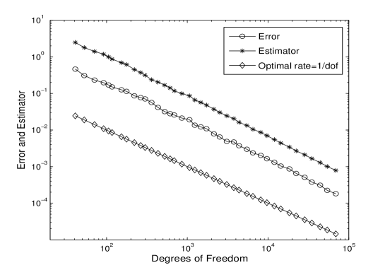
Figure 5.1. Errors and Estimators for Example 1

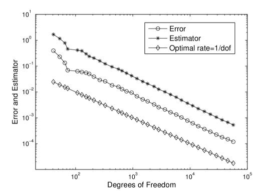
Figure 5.2. Errors and Estimators for Example 2

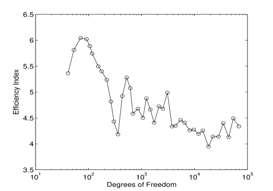
Figure 5.3. Efficiency Index for Example 1

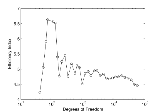
Figure 5.4. Efficiency Index for Example 2

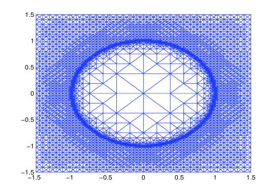
Figure 5.5. Mesh at intermediate level for Example 1

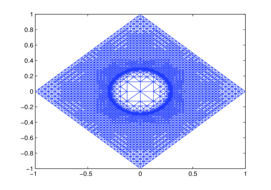
Figure 5.6. Mesh at intermediate level for Example 2

6. Conclusions

For the first time, residual based a posteriori error estimator has been derived for the quadratic finite element method for the elliptic obstacle problem. The estimator is shown to be reliable. The efficiency of the error estimator in this case is less clear than in the case of linear fem, we leave this subject to future investigation. The error estimator involves a discrete Lagrange multiplier which is shown to be optimally convergent to the continuous one whenever the solution $u$, obstacle $\chi$ and the force $f$ are sufficiently smooth and the contact set does not degenerate to a curve in any part of the domain. Also under this assumption, we show that the quadratic fem for obstacle problem is indeed optimal. Numerical experiments with adaptive refinement exhibit this optimal convergence rate.

References

- [1] M. Ainsworth and J. T. Oden. A posteriori error estimation in finite element analysis. Pure and Applied Mathematics (New York). Wiley-Interscience [John Wiley & Sons], New York, 2000.
- [2] K. Atkinson and W. Han. Theoretical Numerical Analysis. A functional analysis framework. Thrid edition, Springer, 2009.
- [3] S. Bartels and C. Carstensen. Averaging techniques yield relaible a posteriori finite element error control for obstacle problems, Numer. Math., 99:225–249, 2004.
- [4] D. Braess. A posteriori error estimators for obstacle problems-another look. Numer. Math., 101:415-421, 2005.
- [5] S.C. Brenner and L.R. Scott. The Mathematical Theory of Finite Element Methods Third Edition. Springer-Verlag, New York, 2008.
- [6] F. Brezzi, W. W. Hager, and P. A. Raviart. Error estimates for the finite element solution of variational inequalities, Part I. Primal theory. Numer. Math., 28:431–443, 1977.
- [7] D. Braess, C. Carstensen and R.H.W. Hoppe. Convergence analysis of a conforming adaptive finite element method for an obstacle problem. Numer. Math., 107:455–471, 2007.
- [8] Z. Chen and R. Nochetto. Residual type a posteriori error estimates for elliptic obstacle problems. Numer. Math., 84:527–548, 2000.
- [9] P.G. Ciarlet. The Finite Element Method for Elliptic Problems. North-Holland, Amsterdam, 1978.
- [10] W. Dörlfer A convergent adaptive algorithm for Poisson’s equation. SIAM J. Numer. Anal., 33:1106–1124, 1996.
- [11] R. S. Falk. Error estimates for the approximation of a class of variational inequalities, Math. Comp., 28:963-971, (1974).
- [12] R. Glowinski. Numerical Methods for Nonlinear Variational Problems. Springer-Verlag, Berlin, 2008.
- [13] T. Gudi and K. Porwal. A posteriori error control of discontinuous Galerkin methods for elliptic obstacle problems, Math. Comput., 83:579–602, 2014.
- [14] T. Gudi and K. Porwal. A remark on the a posteriori error analysis of discontinuous Galerkin methods for obstacle problem, Comput. Meth. Appl. Math., 14:71–87, 2014.
- [15] M. Hintermüller, K. Ito and K. Kunish. The primal-dual active set strategy as a semismooth Newton method. SIAM J. Optim., 13:865–888, 2003.
- [16] D. Kinderlehrer and G. Stampacchia. An Introduction to Variational Inequalities and Their Applications. SIAM, Philadelphia, 2000.
- [17] R. Nochetto, T. V. Petersdorff and C. S. Zhang. A posteriori error analysis for a class of integral equations and variational inequalities. Numer. Math, 116:519–552, 2010.
- [18] A. Veeser. Efficient and Relaible a posteriori error estimators for elliptic obstacle problems. SIAM J. Numer. Anal., 39:146–167, 2001.
- [19] L. Wang. On the quadratic finite element approximation to the obstacle problem. Numer. Math., 92:771–778, 2002.
- [20] F. Wang, W. Han and X.Cheng. Discontinuous Galerkin methods for solving elliptic variational inequalities. SIAM J. Numer. Anal., 48:708–733, 2010.
- [21] A. Weiss and B. I. Wohlmuth A posteriori error estimator for obstacle problems. SIAM J. Numer. Anal., 32:2627–2658, 2010.