The generating function for the connected correlator in the random energy model and its effective potential

Abstract

Starting with two copies of the random energy model coupled with independent magnetic fields, the generating function for the connected correlator of the magnetization is exactly derived. Without use of the replica trick, it is shown that the Hessian of the generating function is symmetric under exchanging the two copies when the system is finite, but the symmetry is spontaneously broken in the low-temperature phase. It can be regarded as a rigorous realization of the replica symmetry breaking. The corresponding effective potential, which has two independent variables conjugate to the magnetic fields, is also calculated. It is singular when the two variables coincide. The singularity is consistent with that observed in the effective potentials of short-ranged disordered systems in the context of the functional renormalization group.

I Introduction

A technical difficulty in theoretical study of quenched disordered systems originates from inhomogeneity due to disordered environment. In those systems, we first take the thermal average of physical quantities in a fixed disordered environment and then we need to take the average over the disorder. However, if we can first average out the disorder, problems in those systems will be more tractable. Several methods to make it possible are developed in the last four decades and they expose peculiarities in quenched disordered systems.

One of the most popular method will be the replica trick MPV87 , where identical $n$ copies (replicas) of the system are introduced. In mean-field models such as the Sherrington-Kirkpatrick model SK75 or the random energy model (REM) D80 ; D81 , glassy behavior is revealed together with the replica symmetry breaking (RSB). In order to show the RSB, the limit $n\to 0$ is taken despite that $n$ is a natural number. The RSB is a peculiar feature of quenched disordered systems in the sense that we do not know a mathematical reason why it gives the correct answer D11 .

Another peculiarity we treat here is that a non-analytic potential appearing as a fixed point of a flow equation of the functional renormalization group (FRG) in short-ranged disorder models F86 ; Fe01 ; LW02 ; TT04 ; WL07 ; LMW08 ; TT08 . Because of a semi-quantitative argument why the non-analytic fixed point appears and of consistency with other methods WL07 , existence of the non-analyticity in the fixed-point potential is quite plausible. However, we do not know its robustness against higher-order corrections to the flow equation.

Therefore it is worthwhile to clearly show existence of these peculiarities in disordered systems by solving a simple model exactly. In this paper, dealing with the REM, we derive the exact generating function for the connected two-point function of the magnetization. In this case, as pointed out in the literature LW02 ; TT04 ; LMW08 ; TT08 , we need to introduce two copies of the REM coupled with independent external sources and to take the average over disorder. Here, we do not use the replica trick for mathematical justification, but use the normalized partition function. The validity of the normalization in quenched disordered systems is emphasized in Refs. WL07, ; KL09, , and is realized by the Keldysh formalism CLN99 or by the supersymmeric method W05 . In the REM, it is simply carried out using an integral representation of the normalization factor.

The generating function obtained in this way is symmetric under the exchanging the two external sources. However, computing the Hessian of this function, we can show in the low-temperature phase that the symmetry is spontaneously broken in the usual sense of the statistical machanics. That can be a mathematically well-defined counterpart of the usual RSB. Furthermore, we show that the effective potential, which is obtained by the Legendre transformation of the generating function, becomes non-analytic in accordance with the symmetry breaking. It is quite similar to the result in study of random manifolds employing the functional renormalization group LW02 ; LMW08 .

This paper is organized as follows: in the next section, we recall the definition of the REM in a uniform magnetic field and define the generating function for connected correlation functions of the total magnetization. We also review that $n$ copies of the system independently coupled with magnetic fields are needed for deriving the $n$-point correlation function LW02 ; TT04 ; LMW08 ; TT08 . In section III, we calculate the exact generating function for the connected two-point function when the system is finite. We see that it has a symmetry exchanging two copies of the system. As a result, the Hessian of the generating function becomes a replica symmetric matrix at the zero-magnetic field. In section IV, we study the asymptotic behavior of the generating function when the system approaches the thermodynamic limit. If the magnetic fields are turned off after the thermodynamic limit is taken, the Hessian is not replica symmetric anymore in the low-temperature phase. It means that the symmetry is spontaneously broken. In section V, performing the Legendre transformation to the generating function in the thermodynamic limit, we obtain the exact effective potential. Corresponding to the two external sources in the generating function, the effective potential has two independent variables, $\varphi_{1}$ and $\varphi_{2}$. We show that it is analytic in the high-temperature phase, while it is singular on $\varphi_{1}\varphi_{2}=0$ or on $\varphi_{1}=\varphi_{2}$ in the low temperature phase. A physical interpretation of this singularity is also presented. The last section is devoted to summary and discussion.

II The REM in a magnetic field and its generating function

The random energy model (REM) is defined on configurations of $N$ spins $\{\sigma_{i}\}$, $(i=1,...,N)$, each of which takes the values of $\pm 1$. When there is no external field, the energy $E$ of a spin configuration is completely independent of how the configuration is. It just follows a gaussian probability density $P(E)$ describing disorder environment. When a uniform magnetic field $H$ is turned on, the energy $E$ gets dependence on the magnetization $M:=\sum_{i=1}^{N}\sigma_{i}$ and is modified to $E-HM$.

For a precise description, it is convenient to classify all the spin configurations by values of $M$ DW01 . Since the number of the configurations with the magnetization $M$ is $n(M):=\binom{N}{(N+M)/2}$, we can label all the states with the two numbers $M$ and $k$, where $M\in\{-N,-N+2,...,N-2,N\}$ and $k\in\{1,2,...,n(M)\}$. The energy of the state labelled by $(M,k)$ is $E_{M,k}-HM$. Here $E_{M,k}$ is a random variable obeying the following gaussian probability density independent of $M$ and $k$:

$$P(E_{M,k}):=\frac{1}{\sqrt{\pi NJ^{2}}}\exp\left(-\frac{E_{M,k}^{2}}{NJ^{2}}\right),$$ (1)

which defines the average over disorder. We denote it by the overline as

$$\overline{X}:=\int\prod_{M}\prod_{k=1}^{n(M)}P(E_{M,k})\,X\,dE_{M,k}.$$ (2)

The partition function is given by

$$Z(H):=\sum_{M}\sum_{k=1}^{n(M)}e^{-\beta E_{M,k}+\beta MH}.$$ (3)

Note that $\sum_{M}n(M)$ equals the total number of configurations $2^{N}$.

Let us obtain the generating function for the disorder average of the connected correlation functions of $M$. If we ignore the average over the disorder, the generating function is given by $\beta^{-1}\log Z(H)$. Taking the derivative with respect to $H$, we can obtain connected correlation functions of $M$. However, taking into account the random average, if we start with $\overline{Z(H)}$, we have to take care of a couple of things. To see this, taking the derivative of $\log\overline{Z(H)}$, one finds that

$$\beta^{-1}\left.\frac{\partial\log\overline{Z(H)}}{\partial H}\right|_{H=0}=\frac{\overline{\left\langle M\right\rangle Z(0)}}{\overline{Z(0)}},$$ (4)

where the angle brackets denotes the thermal average with zero-magnetic field as follows:

$$\left\langle X\right\rangle:=\frac{1}{Z(0)}\sum_{k=1}^{n(M)}Xe^{-\beta E_{M,k}}.$$ (5)

The result (4) differs from the one-point function. One of the usual ways of getting around the problem is the replica trick. Namely, we use the partition function for $n$ ($n$ is a positive integer) copies of the model $\overline{Z(H)^{n}}$ instead of $\overline{Z(H)}$. Define the generating function by $(\beta n)^{-1}\log\overline{Z(H)^{n}}$. After taking the derivative, letting $n\to 0$, we formally obtain the correct one-point function. However, taking the limit $n\to 0$ is not a procedure mathematically justified, so that we do not use it in the present paper. Instead, we use the normalized partition function defined as

$$z(H):=\frac{Z(H)}{Z(0)}.$$ (6)

Inserting $z(H)$ instead of $Z(H)$ in (4) and using the normalization condition $z(0)=1$, we can obtain the correct one-point function.

However, it is not enough to obtain the correlation functions. In fact, taking the second derivative, we find that

$$\left.\beta^{-2}\frac{\partial^{2}\log\overline{z(H)}}{\partial H^{2}}\right|_{H=0}=\overline{\left\langle M^{2}\right\rangle}-\overline{\left\langle M\right\rangle}\ \overline{\left\langle M\right\rangle},$$ (7)

which is not the disorder average of the connected two-point function. In order to obtain the correct one, we introduce two copies of the system coupled with independent magnetic fields LW02 ; TT04 ; LMW08 ; TT08 . Namely, we define

$$W(H_{1},H_{2}):=\beta^{-1}\log\overline{z(H_{1})z(H_{2})}.$$ (8)

Then it is easily seen that

$$\beta^{-1}\left.\partial_{1}^{2}W(H_{1},H_{2})\right|_{H_{1}=H_{2}=0}=\overline{\left\langle M^{2}\right\rangle}-\overline{\left\langle M\right\rangle}\ \overline{\left\langle M\right\rangle}$$

$$\beta^{-1}\left.\partial_{1}\partial_{2}W(H_{1},H_{2})\right|_{H_{1}=H_{2}=0}=\overline{\left\langle M\right\rangle^{2}}-\overline{\left\langle M\right\rangle}\ \overline{\left\langle M\right\rangle},$$ (9)

where $\partial_{a}$ $(a=1,2)$ means the derivative with respect to $H_{a}$. We obtain the connected two-point function from the right-hand side of the following formula:

$$\overline{\left\langle M^{2}\right\rangle-\left\langle M\right\rangle^{2}}=\beta^{-1}\left.\left(\partial_{1}^{2}W(H_{1},H_{2})-\partial_{1}\partial_{2}W(H_{1},H_{2})\right)\right|_{H_{1}=H_{2}=0}.$$ (10)

In general, if we want to generate the connected $n$-point function, we need the following generalization of (8):

$$W(H_{1},...,H_{n}):=\beta^{-1}\log\overline{\prod_{k=1}^{n}z(H_{k})}.$$ (11)

For deriving the connected $m$-point function with $m<n$, we may just put $H_{m+1}=\cdots=H_{n}=0$. Thus, $W(H_{1},...,H_{n})$ contains all information up to the $n$-point functions. In this paper we investigate the simplest but nontrivial case, $n=2$.

III The generating function in the finite system

Now let us derive the generating function (8). From the definition (6), we have

$$\overline{z(H_{1})z(H_{2})}=\overline{\left(\frac{Z(H_{1})Z(H_{2})}{Z(0)^{2}}\right)}.$$ (12)

The denominator makes the computation difficult. There are a couple of ways of ensuring the normalization condition such as the Schwinger-Keldysh approach CLN99 ; KL09 or the supersymmetric method W05 . In the REM, it can be established using the following representation:

$$\frac{1}{Z(0)^{2}}=\int_{0}^{\infty}\,t\,e^{-tZ(0)}dt.$$ (13)

Then we have

$$\overline{z(H_{1})z(H_{2})}=\int_{0}^{\infty}dt\,t\ \overline{Z(H_{1})Z(H_{2})\,e^{-tZ(0)}}.$$ (14)

The function $\overline{e^{-tZ(0)}}$ is first introduced by Derrida D81 and studied in detail. Namely, using the fact that the energies $\{E_{M,k}\}$ follow the probability density (1) independently, we can write

$$\overline{e^{-tZ(0)}} = \overline{\prod_{M}\prod_{k=1}^{n(M)}e^{-te^{-\beta E_{M,k}}}}=\prod_{M}\prod_{k=1}^{n(M)}\overline{e^{-te^{-\beta E_{M,k}}}}$$ (15)

$$= \left(f(t)\right)^{2^{N}},$$

where

$$f(t):=\overline{e^{-te^{-\beta E_{M,k}}}}.$$ (16)

By definition, it is immediately derived that

$$f^{\prime}(t) = -\overline{e^{-\beta E_{M,k}-te^{-\beta E_{M,k}}}}$$

$$f^{\prime\prime}(t) = \overline{e^{-2\beta E_{M,k}-te^{-\beta E_{M,k}}}}.$$ (17)

Using (15), (17) and (3) in the right-hand side of (14), we find that

$$\overline{z(H_{1})z(H_{2})}=2^{-N}\sum_{M}e^{\beta(H_{1}+H_{2})M}\,n(M)\,J_{N}+2^{-2N}\sum_{M_{1},M_{2}}e^{\beta(H_{1}M_{1}+H_{2}M_{2})}\,n(M_{1})n(M_{2})I_{N},$$ (18)

where

$$J_{N} := 2^{N}\int_{0}^{\infty}dt\,t\,\left(f^{\prime\prime}(t)\left(f(t)\right)^{2^{N}-1}-f^{\prime}(t)^{2}\left(f(t)\right)^{2^{N}-2}\right)$$

$$I_{N} := 2^{2N}\int_{0}^{\infty}dt\,t\,f^{\prime}(t)^{2}\left(f(t)\right)^{2^{N}-2}.$$ (19)

Setting $H_{1}=H_{2}=0$ in (18), we see the following relationship between $I_{N}$ and $J_{N}$:

$$1=\overline{z(0)z(0)} = J_{N}+I_{N}.$$ (20)

As a result, we can write

$$\overline{z(H_{1})z(H_{2})}=A+B$$ (21)

with

$$A := 2^{-N}(1-I_{N})\sum_{M}e^{\beta(H_{1}+H_{2})M}\,n(M)$$

$$B := 2^{-2N}I_{N}\sum_{M_{1},M_{2}}e^{\beta(H_{1}M_{1}+H_{2}M_{2})}n(M_{1})n(M_{2}).$$ (22)

Thus, the generating function defined in (8) is written as $W(H_{1},H_{2})=\beta^{-1}\log(A+B)$. Hereafter, we treat its density defined by

$$w_{N}(H_{1},H_{2}):=\frac{1}{N}W(H_{1},H_{2})=\frac{1}{N\beta}\log\left(A+B\right)$$ (23)

instead of $W(H_{1},H_{2})$ itself.

From (22) and (23), it is obvious that $w_{N}(H_{1},H_{2})$ is symmetric under exchanging $H_{1}$ and $H_{2}$. This yields the fact that the coefficient of $H_{1}^{k}H_{2}^{l}$ in $w_{N}(H_{1},H_{2})$ must be the same as that of $H_{1}^{l}H_{2}^{k}$ for arbitrary non-negative integers $k$ and $l$. It means that

$$\partial_{1}^{k}\partial_{2}^{l}w_{N}(0,0)=\partial_{1}^{l}\partial_{2}^{k}w_{N}(0,0).$$ (24)

In particular, the Hessian matrix of $w_{N}(H_{1},H_{2})$ defined by

$$w^{(2)}_{N}(H_{1},H_{2})_{ab}:=\partial_{a}\partial_{b}w_{N}(H_{1},H_{2})$$ (25)

must be a replica symmetric matrix. We can explicitly derive it employing the formula

$$\sum_{M}Mn(M)=0,\ \ \sum_{M}M^{2}n(M)=N2^{N}.$$ (26)

The result is

$$w^{(2)}_{N}(0,0)=\left(\begin{array}[]{cc}\beta&\beta(1-I_{N})\\ \beta(1-I_{N})&\beta\end{array}\right)$$ (27)

for an arbitrary finite $N$.

Let us call the two copies of the REM considered here the copy 1 and the copy 2. Suppose that they are respectively coupled with $H_{1}$ and $H_{2}$. Exchanging $H_{1}$ and $H_{2}$ means exchanging the two copies 1 and 2. Thus the above symmetry is similar to the usual replica symmetry.

IV Asymptotic form of $w_{N}(H_{1},H_{2})$ for large $N$ and the symmetry breaking

In this section, we calculate the asymptotic form of $w_{N}(H_{1},H_{2})$ for large $N$. Taking the thermodynamic limit before turning the magnetic fields off, we show that the symmetry exchanging the copies 1 and 2 is spontaneously broken.

IV.1 Evaluation of $I_{N}$

The asymptotic value of $I_{N}$ for large $N$ defined in (19) is calculated with use of properties of $f(t)$ clarified in Refs. D81, ; GD89, . The result is

$$I_{N}\simeq\left\{\begin{array}[]{ll}1&(\beta<\beta_{c})\\ \frac{\beta_{c}}{\beta}&(\beta>\beta_{c}),\end{array}\right.$$ (28)

where $\beta_{c}:=2\sqrt{\log 2}/J$ is the critical temperature. The calculation deriving (28) is lengthy, so that we show it in Appendix. In the main text, we derive the same result with help of the susceptibility $\chi$ of the REM obtained by Derrida D81 :

$$\chi=\lim_{N\to\infty}\frac{\beta}{N}\overline{\left\langle M^{2}\right\rangle-\left\langle M\right\rangle^{2}}=\left\{\begin{array}[]{ll}\beta&(\beta<\beta_{c})\\ \beta_{c}&(\beta>\beta_{c}).\end{array}\right.$$ (29)

From (10) and (23) we see that $\chi$ is calculated as

$$\chi=\lim_{N\to\infty}\left(\partial_{1}^{2}w_{N}(0,0)-\partial_{1}\partial_{2}w_{N}(0,0)\right)$$ (30)

in our formulation. For sufficiently large $N$, the summations in $A$ and $B$ can be evaluated by their extremum. Namely,

$$A \simeq \left(1-I_{N}\right)e^{N(s(m^{*})+\beta(H_{1}+H_{2})m^{*})},$$

$$B \simeq I_{N}e^{N(s(m_{1}^{*})+\beta H_{1}m_{1}^{*}+s(m_{2}^{*})+\beta H_{2}m_{2}^{*})}.$$ (31)

In (31), $s(m)$ is the following asymptotic form of $n(M)2^{-N}$ with fixed $m:=M/N$:

$$s(m):=-\frac{1}{2}\left(\left(1-m\right)\log\left(1-m\right)+\left(1+m\right)\log\left(1+m\right)\right),$$ (32)

and

$$m^{*} := \tanh\beta(H_{1}+H_{2}),$$

$$m^{*}_{a} := \tanh\beta H_{a}\qquad(a=1,2),$$ (33)

which are respectively the solutions of the the extremum conditions

$$s^{\prime}(m^{*})+\beta(H_{1}+H_{2})=0,\qquad s^{\prime}(m_{a}^{*})+\beta H_{a}=0.$$ (34)

Using (31), (33) and (34) in (23), we find the following asymptotic forms of the first and the second derivatives of $w_{N}(H_{1},H_{2})$ for large $N$:

$$\partial_{a}w_{N}(H_{1},H_{2}) \simeq \frac{m^{*}A+m^{*}_{a}B}{A+B}$$

$$\partial_{a}^{2}w_{N}(H_{1},H_{2}) \simeq \frac{\beta}{A+B}\left(A(1-m^{*2})+B\left(1-m_{a}^{*2}\right)\right)+\frac{N\beta AB\left(m^{*}-m_{a}^{*}\right)^{2}}{(A+B)^{2}}$$

$$\partial_{1}\partial_{2}w_{N}(H_{1},H_{2}) \simeq \frac{\beta A\left(1-m^{*2}\right)}{A+B}+\frac{N\beta(m^{*}-m_{1}^{*})(m^{*}-m_{2}^{*})AB}{(A+B)^{2}},$$ (35)

where $a=1,2$. Since $A=1-I_{N},B=I_{N},m^{*}=m^{*}_{1}=m^{*}_{2}=0$ when $H_{1}=H_{2}=0$, we can readily calculate (30) as

$$\chi=\lim_{N\to\infty}\left((\beta-\beta(1-I_{N})\right)=\beta\lim_{N\to\infty}I_{N}.$$ (36)

Comparing (36) with the known result (29), we obtain (28).

IV.2 RSB-like Symmetry breaking

Now we derive the asymptotic form of the Hessian matrix defined by (25). In the high-temperature phase, $\beta<\beta_{c}$, we find from (28) and (31) that $A$ vanishes in (35). Thus, we get

$$\beta^{-1}w_{N}^{(2)}(H_{1},H_{2})\simeq\left(\begin{array}[]{cc}1-m_{1}^{*2}&0\\ 0&1-m_{2}^{*2}\end{array}\right)$$ (37)

for sufficiently large $N$.

In the low-temperature phase, $\beta>\beta_{c}$, we compare the exponent of $A$ and $B$ introducing

$$g(H_{1},H_{2}) := s(m^{*})+\beta\left(H_{1}+H_{2}\right)m^{*}$$ (38)

$$-\sum_{a=1}^{2}\left(s(m_{a}^{*})+\beta H_{a}m_{a}^{*}\right).$$

We see from (31) that $g(H_{1},H_{2})\simeq(\log A-\log B)/N$. For fixed $H_{2}>0$, we can show that the function of $H$, $g(H,H_{2})$, is monotone increasing and $g(0,H_{2})=0$. It means that $A$ exponentially dominates over $B$ when $H_{1}>0$ and $H_{2}>0$. On the other hand, $B$ exponentially dominates over $A$ when $H_{1}<0$ and $H_{2}>0$. Similar calculation leads to

$$\begin{array}[]{ll}\frac{1}{N}\log A>\frac{1}{N}\log B&(H_{1}H_{2}>0)\\[5.69054pt] \frac{1}{N}\log A<\frac{1}{N}\log B&(H_{1}H_{2}<0)\\[5.69054pt] \frac{1}{N}\log A\simeq\frac{1}{N}\log B&(H_{1}H_{2}=0)\end{array}$$ (39)

for large $N$. It means that, when $H_{1}H_{2}>0$,

$$\frac{A}{A+B}\to 1,\ \ \frac{B}{A+B}\to 0$$ (40)

in (35) for example. Applying similar formulas, we get

(i) for $H_{1}H_{2}>0$,

$$\beta^{-1}w_{N}^{(2)}(H_{1},H_{2})\simeq\left(\begin{array}[]{cc}1-m^{*2}&1-m^{*2}\\ 1-m^{*2}&1-m^{*2}\end{array}\right)$$ (41)

(ii) for $H_{1}H_{2}<0$,

$$\beta^{-1}w_{N}^{(2)}(H_{1},H_{2})\simeq\left(\begin{array}[]{cc}1-m_{1}^{*2}&0\\ 0&1-m_{2}^{*2}\end{array}\right)$$ (42)

(iii) for $H_{1}=0$,

$$\beta^{-1}w_{N}^{(2)}(0,H_{2})\simeq\left(\begin{array}[]{cc}1-(1-I_{N})\,m_{2}^{*2}+NI_{N}(1-I_{N})\,m_{2}^{*2}&\ (1-I_{N})(1-m_{2}^{*2})\\ (1-I_{N})(1-m_{2}^{*2})&1-m_{2}^{*2}\end{array}\right)$$ (45)

(iv) for $H_{2}=0$,

$$\beta^{-1}w_{N}^{(2)}(H_{1},0)\simeq\left(\begin{array}[]{cc}1-m_{1}^{*2}&(1-I_{N})(1-m_{1}^{*2})\\ (1-I_{N})(1-m_{1}^{*2})&\ 1-(1-I_{N})\,m_{1}^{*2}+NI_{N}(1-I_{N})\,m_{1}^{*2}\end{array}\right).$$ (46)

Now we consider the symmetry transformation exchanging the two copies 1 and 2 coupled with $H_{1}$ and $H_{2}$ respectively. For finite $N$, the symmetry ensures that $w_{N}^{(2)}(0,0)$ is a replica symmetric matrix as we have seen in (27). To see the spontaneous symmetry breaking, we first put the symmetry breaking field $(H_{1},H_{2})=(H,0)$, then take the thermodynamic limit $N\to\infty$, and finally turn off $H$. In the high-temperature phase, using (37), we have

$$\lim_{H\to 0}\lim_{N\to\infty}w^{(2)}_{N}(H,0)=\left(\begin{array}[]{cc}\beta&0\\ 0&\beta\end{array}\right).$$ (47)

It implies that the symmetry exchanging the copies holds in the high-temperature phase. On the other hand, in the low-temperature phase, it is found from (46) that

$$\lim_{H\to 0}\lim_{N\to\infty}w^{(2)}_{N}(H,0)=\left(\begin{array}[]{cc}\beta&\beta-\beta_{c}\\ \beta-\beta_{c}&+\infty\end{array}\right).$$ (48)

It is no longer a replica symmetric matrix, so that the symmetry exchanging the two copies is spontaneously broken in the usual sense of the statistical machenics. The symmetry breaking is reminiscent of the RSB in which the zero-replica limit not mathematically justified is inevitable MM09 . The symmetry breaking presented here can be a mathematically well-defined counterpart to the RSB.

It is worthwhile exploring the surface defined by $z=w_{N}(H_{1},H_{2})$ in the thermodynamic limit for understanding the broken symmetry. Let us define

$$w(H_{1},H_{2}):=\lim_{N\to\infty}w_{N}(H_{1},H_{2})=\lim_{N\to\infty}\frac{1}{N\beta}\log(A+B).$$ (49)

In the high-temperature phase, $A$ vanishes in (49) since $I_{N}\to 1$ as $N\to\infty$ according to (28). We immediately find from (31) that

$$w(H_{1},H_{2})=\sum_{a=1}^{2}\left(\frac{s(m_{a}^{*})}{\beta}+H_{a}m_{a}^{*}\right)$$ (50)

for all $H_{1}$ and $H_{2}$. It is analytic and derives (47). Using the relationship (39), we can derive $w(H_{1},H_{2})$ in the low-temperature phase in a similar manner. The result is

$$w(H_{1},H_{2})=\left\{\begin{array}[]{ll}\frac{1}{\beta}s(m^{*})+(H_{1}+H_{2})m^{*}&(H_{1}H_{2}\geq 0)\\[5.69054pt] \sum_{a=1}^{2}\left(\frac{1}{\beta}s(m_{a}^{*})+H_{a}m_{a}^{*}\right)&(H_{1}H_{2}<0)\\[5.69054pt] \end{array}\right..$$ (53)

It is continuous on the whole $H_{1}H_{2}$ plane. When $H_{1}H_{2}\neq 0$, $w(H_{1},H_{2})$ is differentiable and

$$\partial_{a}w(H_{1},H_{2})=\left\{\begin{array}[]{ll}m^{*}&(H_{1}H_{2}>0)\\ m_{a}^{*}&(H_{1}H_{2}<0)\end{array}\right.\ \ (a=1,2).$$ (54)

It shows that $\partial_{a}w(H_{1},H_{2})$ $(a=1,2)$ is discontinuous on $H_{a}=0$ except the origin. For example, when $H>0$, we get

$$\lim_{H_{2}\uparrow 0}\partial_{2}w(H,H_{2}) = \lim_{H_{2}\uparrow 0}m_{2}^{*}=0,$$

$$\lim_{H_{2}\downarrow 0}\partial_{2}w(H,H_{2}) = \left.m^{*}\right|_{H_{1}=H,H_{2}=0}$$ (55)

$$= \tanh\left(\beta H\right)\neq 0.$$

This non-differentiability, which is depicted in Fig.1, leads to $\partial_{2}^{2}w(H,0)=+\infty$ in (48). On the other hand, since $w(H,0)$ is infinitely many-times differentiable with respect to $H$, $\partial_{1}^{2}w(H,0)<\infty$. It indicates that the diagonal part of the Hessian differs each other at $(H_{1},H_{2})=(H,0)$ for an arbitrary $H\neq 0$, which results in the spontaneously symmetry breaking.

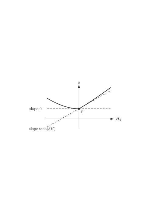
Figure 1: The solid curve is $z=w(H,H_{2})$ with fixed $H>0$. The dashed lines represent tangential lines at P$(H,0,w(H,0))$ in the $H_{1}H_{2}z$ space. The slopes $0$ and $\tanh(\beta H)$ are respectively the left and the right derivative at $H_{2}=0$, which correspond to the spontaneous magnetization in the copy 2 in presence of the magnetic field $H$ in the copy 1.

A physical picture of this non-differentiability will be explained as follows: first we set $H_{1}=H_{2}=0$. In order to obtain a magnetization in the copy 1, we need to put a finite external field $H$ to the copy 1, which yields the magnetization $m_{1}=\tanh(\beta H)$. It means that the copy 1 shows paramagnetism. Next, we put an infinitesimal magnetic field $H_{2}$ to the copy 2. If $H_{2}$ has the same direction as $H$ ($HH_{2}>0$), the copy 2 has the spontaneous magnetization with just the same value as $m_{1}$. On the other hand, if $H_{2}$ has the opposite direction as $H$, the copy 2 has no longer finite magnetization. In this way, a value of the spontaneous magnetization is different depending on a direction of the infinitesimal magnetic field, which results in the non-differentiability. This picture implies the meaning of the broken symmetry exchanging 1 and 2. Namely, if we want to magnetize both the copy 1 and the copy 2, we need to apply a finite external field to one copy, while it is sufficient to apply an infinitesimal field to the other copy.

V The Effective Potential

In this section, we derive the effective potential $\gamma(\varphi_{1},\varphi_{2})$ conjugate to $w(H_{1},H_{2})$, which is defined by the following Legendre transformation

$$\gamma(\varphi_{1},\varphi_{2}):=\max_{H_{1},H_{2}}\left(\varphi_{1}H_{1}+\varphi_{2}H_{2}-w\left(H_{1},H_{2}\right)\right).$$ (56)

Here, if $w(H_{1},H_{2})$ is differentiable, the maximization can be carried out by solving the following equations

$$\varphi_{a}=\partial_{a}w(H_{1},H_{2}),\ \ (a=1,2)$$ (57)

for $H_{1}$ and $H_{2}$, and then inserting the solutions into the right-hand side of (56).

In the high-temperature phase, $w(H_{1},H_{2})$ is given by the formula (50). Using the extremum condition (34), we get

$$\varphi_{a}=m_{a}^{*},\ \ (a=1,2)$$ (58)

for all $H_{1}$ and $H_{2}$. Solving them for $H_{1}$ and $H_{2}$, we obtain

$$\gamma(\varphi_{1},\varphi_{2})=-\frac{1}{\beta}\sum_{a=1}^{2}s(\varphi_{a}).$$ (59)

It has the global minimum at the origin and has no singularity.

In the low-temperature phase, using (53) and (54), we can derive $\gamma(\varphi_{1},\varphi_{2})$ in a similar manner. We have

$$\gamma(\varphi_{1},\varphi_{2})=\left\{\begin{array}[]{ll}-\frac{1}{\beta}s(\varphi_{a}),&(\varphi_{1}=\varphi_{2})\\ -\frac{1}{\beta}\sum_{a=1}^{2}s(\varphi_{a})&(\varphi_{1}\varphi_{2}<0)\end{array}\right..$$ (60)

In the above formula, note that the domain defined by $H_{1}H_{2}>0$ maps to the line $\varphi_{1}=\varphi_{2}$. In order to determine $\gamma(\varphi_{1},\varphi_{2})$ for all $\varphi_{1}$ and $\varphi_{2}$ ($|\varphi_{a}|<1,\,a=1,2)$, we have to investigate the case of $H_{1}H_{2}=0$. In this case, a partial derivative does not exist as we have seen in the previous section, so that we employ the following geometrical meaning of the Legendre transformation (56): for a given $\varphi_{1}$ and $\varphi_{2}$, consider the plane defined by the following formula

$$z=\varphi_{1}H_{1}+\varphi_{2}H_{2}+z_{0}$$ (61)

in the $H_{1}H_{2}z$ space. We choose $z_{0}$ in such a way that the plane has a common point with the surface $z=w(H_{1},H_{2})$ and try to minimize the value of $z_{0}$. The minimum value of $z_{0}$ gives $-\gamma(\varphi_{1},\varphi_{2})$.

First we consider the case of $H_{2}=0$. Take an arbitrary point $(H,0)$ on the line and consider the corresponding point $\textrm{P}(0,H,w(H,0))$ on the surface $z=w(H_{1},H_{2})$. Choosing $\varphi_{1}$, $\varphi_{2}$ and $z_{0}$ in (61) appropriately, we construct a plane contacting with the surface $z=w(H_{1},H_{2})$ at P. Since $\partial_{1}w(H,0)$ is well-defined according to (53), $\varphi_{1}$ is uniquely determined as

$$\varphi_{1}=\partial_{1}w(H,0)=\left.m^{*}\right|_{H_{1}=H,H_{2}=0}=\tanh(\beta H).$$ (62)

On the other hand, $\partial_{2}w(H,0)$ does not exist as we have seen in (55). In this case, $\varphi_{2}$ can take the value between the left and the right derivative, namely, 0 and $\tanh(\beta H)=\varphi_{1}$. Since the point P is on the plane (61), we find that $z_{0}=w(H,0)-\varphi_{1}H=s(\varphi_{1})/\beta$. See Fig 2. Consequently the plane (61) contacts with $z=w(H_{1},H_{2})$ at P if $\varphi_{1}=\tanh(\beta H)$, $z_{0}=s(\varphi_{1})/\beta$, and $\varphi_{2}$ is a value between 0 and $\varphi_{1}$.

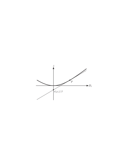
Figure 2: The sectional plane $H_{2}=0$ in the $H_{1}H_{2}z$ space. The solid line is the cross section of the surface $z=w(H_{1},H_{2})$. The dashed line represents the the plane $z=\varphi_{1}H_{1}+\varphi_{2}H_{2}+z_{0}$ contacting with the surface at $\textrm{P}(H,0,w(H,0))$. It intercepts the $z$ axes at $s(\varphi_{1})/\beta$, which is equal to $-\gamma(\varphi_{1},\varphi_{2})$.

Note that if $z_{0}$ took a value less than $s(\varphi_{1})/\beta$, the plane (61) would not have a common point with the surface. Thus we conclude that

$$\gamma\left(\varphi_{1},\varphi_{2}\right)=-s(\varphi_{1})/\beta$$ (63)

for $\varphi_{2}\in[0,\varphi_{1}]$ or $\varphi_{2}\in[\varphi_{1},0]$.

When $H_{1}=0$, exchanging the role of $\varphi_{1}$ and $\varphi_{2}$ in the case of $H_{2}=0$, we get

$$\gamma\left(\varphi_{1},\varphi_{2}\right)=-s(\varphi_{2})/\beta$$ (64)

for $\varphi_{1}\in[0,\varphi_{2}]$ or $\varphi_{1}\in[\varphi_{2},0]$.

Combining the results (60) (63) and (64), we finally obtain

$$\gamma(\varphi_{1},\varphi_{2})=\left\{\begin{array}[]{ll}-\frac{1}{\beta}s(\varphi_{1})&(0\leq\varphi_{2}\leq\varphi_{1}\ \textrm{or}\ \varphi_{1}\leq\varphi_{2}\leq 0)\\[5.69054pt] -\frac{1}{\beta}s(\varphi_{2})&(0\leq\varphi_{1}\leq\varphi_{2}\ \textrm{or}\ \varphi_{2}\leq\varphi_{1}\leq 0)\\[5.69054pt] -\frac{1}{\beta}\sum_{a=1}^{2}s(\varphi_{a})&(\varphi_{1}\varphi_{2}<0)\end{array}\right..$$ (65)

As is shown in Fig.3, regions that specify the values of $\gamma(\varphi_{1},\varphi_{2})$ have the boudaries $\varphi_{a}=0$ $(a=1,2)$ and $\varphi_{2}=\varphi_{1}$, on which it is continuous but non-analytic.

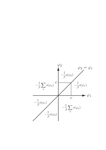
Figure 3: Values of $\gamma(\varphi_{1},\varphi_{2})$ on the $\varphi_{1}\varphi_{2}$ plane. The segments on $\varphi_{1}=c$ or $\varphi_{2}=c$ show a contour with the value $\gamma(\varphi_{1},\varphi_{2})=-\frac{1}{\beta}s(c)$. They meet at $\varphi_{1}=\varphi_{2}=c$, where the effective potential becomes singular. See also Fig. 5.

The non-analyticity on $\varphi_{1}=\varphi_{2}$ is similar to behavior observed in fixed-point potentials of the FRG in various disordered systems F86 ; Fe01 ; LW02 ; TT04 ; WL07 ; LMW08 ; TT08 . Because of a property of disorder correlators in that literature, the potential term in a replicated Hamiltonian depends on the variable $|\varphi_{1}-\varphi_{2}|$ and has a singularity at $|\varphi_{1}-\varphi_{2}|=0$. Hence it is helpful for comparison to introduce the variables $x:=(\varphi_{2}-\varphi_{1})/2$ and $y:=(\varphi_{2}+\varphi_{1})/2$. For fixed $y>0$ and for small $x$ satisfying $|x|<y$, the effective potential is written as

$$\gamma(\varphi_{1},\varphi_{2})=-\frac{1}{\beta}s\left(y+|x|\right).$$ (66)

We see the singularity at $x=0$, which is similar to the fixed-point potential in the random $O(N)$ model studied in LW02 .

Now we consider a physical picture suggested by the singularities including $\varphi_{1}=0$ or $\varphi_{2}=0$. Let us recall a form of an effective potential in $Z_{2}$ symmetric (pure) spin theory. It is well known that a minimizer of the effective potential gives the value of spontaneous magnetization. In the low-temperature phase, the classical potential has a shape of a double well. However, since the effective potential must be a convex function, it has a flat bottom as depicted in Fig. 4 G92 .

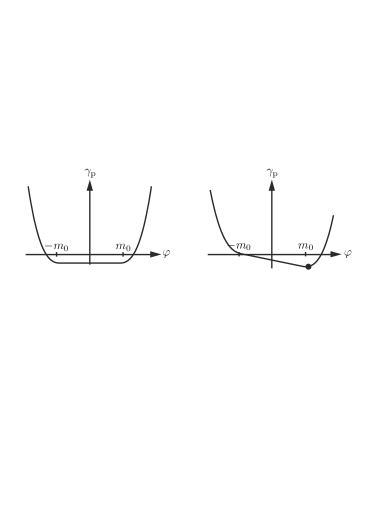
Figure 4: A form of the effective potential $\gamma_{\textrm{p}}(\varphi)$ of a pure $Z_{2}$ spin theory (left). It has a flat bottom $-m_{0}\leq\varphi\leq m_{0}$. In order to take a unique minimizer, we put an infinitesimal magnetic field $H$ which yields the additional term $-\varphi\,H$ to $\gamma_{\textrm{p}}(\varphi)$, thus the shape of the effective potential becomes the right figure. The unique minimizer denoting the dot in the figure approaches $m_{0}$ as $H\to 0$.

In order to take a unique minimizer, we need to turn on an infinitesimal magnetic field. The resultant minimizer is a function of the magnetic field and does not vanish after the magnetic field is turned off. It corresponds to the value of the spontaneous magnetization.

Now we apply the idea to $\gamma(\varphi_{1},\varphi_{2})$ in the low-temperature phase. It is found from (65) that $\gamma(\varphi_{1},\varphi_{2})$ has a unique minimum at the origin, which corresponds to the fact that there is no spontaneous magnetization. First a magnetic field is turned on to the copy 1 in such a way that the minimizer is shifted to $(\varphi_{1},\varphi_{2})=(c,0)$ $(c\neq 0)$. Next an infinitesimal magnetic field having the sign same as $c$ is turned on in the copy 2. As we see from Fig. 5, this yields spontaneous magnetization in the copy 2 with the value $c$, just the same value as in the copy 1. This originates from the non-analyticity on $\varphi_{1}=\varphi_{2}$. However, if the infinitesimal field has the opposite sign to $c$, the value of the magnetization vanishes due to the singularity on $\varphi_{2}=0$.

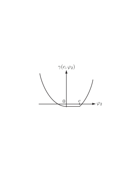
Figure 5: A graph of $\gamma(c,\varphi_{2})$ as a function of $\varphi_{2}$ in the case when $c>0$. We see from (65) that it has a flat bottom $0\leq\varphi_{2}\leq c$. We turn on an infinitesimal magnetic field $H$ for selecting the unique minimizer. If $H>0$, the value of the spontaneous magnetization in the copy 2 is $c$, which is the same value as in the copy 1. On the other hand, if $H<0$, the spontaneous magnetization vanishes.

VI Summary and Discussion

Introducing two copies of the REM coupled with independent magnetic fields, we have calculated the generating function for the correlator of the magnetization. When the system is finite, the Hessian of the generating function at the zero-magnetic fields is a replica symmetric matrix. It reflects the symmetry exchanging the two copies. In the low temperature phase, however, we see that the symmetry is spontaneously broken in the usual sense of the statistical mechanics. In fact, one of the diagonal components of the Hessian becomes infinity while the other remains finite. The asymmetry of the diagonal components is physically interpreted as follows: if we want to magnetize the system, we have to turn on external magnetic field to one copy as in the case of the paramagnetism, while we can see spontaneous magnetization in the other copy.

This broken symmetry reminds us of the usual RSB and may provide a rigorous notion for the RSB. In order to clarify this observation, we need to investigate other disordered systems and show the universality of the broken symmetry presented in this work. If it exists in the various disordered systems, one also has to consider the relationship to the usual RSB and to glassy behavior. We are now planning to study the REM having the ferromagnetic coupling MSxx .

Furthermore, the value of the magnetizations coincide each other if the two magnetic fields, one is finite and the other is infinitesimal for the spontaneous magnetization, have the same direction. Coincidence of the two magnetization reflects the fact that the effective potential corresponding to the generating function has the singularity at which the two independent variables coincide. It supports the fact that singularity of the fixed-point potential of the FRG certainly exists in disordered systems, not the artifact of approximation.

*

Appendix A Asymptotic value of $I_{N}$

In this appendix, we derive the asymptotic value (28) evaluating $f(t)$ defined by (16). It has been first introduced and investigated by Derrida D81 . A similar analysis has been recently performed by Dotsenko D11 in which the same function is called $G(N,x)$. Here, we follow the analysis carried out by Gardner and Derrida GD89 .

Using (1), we can write $f(t)$ as

$$f(t):=\overline{e^{-te^{-\beta E_{M,k}}}}=\frac{1}{\sqrt{\pi}}\int_{-\infty}^{\infty}dy\,e^{-y^{2}-te^{-\lambda y}},$$ (67)

where $\lambda:=\sqrt{N}\beta J$. It has the following asymptotic form depending on ranges of $\log t$ D81 :

$$f(t)\simeq\left\{\begin{array}[]{ll}-k(t)\,e^{-(\log t)^{2}/\lambda^{2}}&(\log t>0)\\[5.69054pt] 1-k(t)\,e^{-(\log t)^{2}/\lambda^{2}}&(-\lambda^{2}/2<\log t<0)\\[5.69054pt] 1-e^{\lambda^{2}/4}t&(\log t<-\lambda^{2}/2)\end{array}\right.,$$ (68)

where $k(t)$ is the function of $t$ defined by

$$k(t):=\frac{-\Gamma\left(\frac{2\log t}{\lambda^{2}}\right)}{\sqrt{\pi}\lambda}.$$ (69)

Although higher-order terms with respect to $t$ are determined when $\log t<-\lambda^{2}/2$ in Ref. D81, , the main terms described in (68) are sufficient in the present study. Introducing $\phi(t)$ by the following formula

$$\exp\left(-\phi(t)\right)=\left(f(t)\right)^{2^{N}},$$ (70)

the integral $I_{N}$ defined in (19) is written as

$$I_{N}=2^{2N}\int_{0}^{\infty}dt\,t\,\left(\frac{f^{\prime}(t)}{f(t)}\right)^{2}e^{-\phi(t)}.$$ (71)

We divide the interval $[0,\infty)\ni t$ into the following three intervals

$$K_{1}:=[0,e^{-\lambda^{2}/2}],\ \ K_{2}:=[e^{-\lambda^{2}/2},1],\ \ K_{3}:=[1,\infty)$$ (72)

in accordance with (68), and evaluate

$$I^{(j)}:=2^{2N}\int_{K_{j}}dt\,t\left(\frac{f^{\prime}(t)}{f(t)}\right)^{2}e^{-\phi(t)},\qquad j=1,2,3$$ (73)

separately. To begin with, we compute

$$I^{(1)}=2^{2N}\int_{0}^{e^{-\lambda^{2}/2}}dt\,t\left(\frac{f^{\prime}(t)}{f(t)}\right)^{2}e^{-\phi(t)},$$ (74)

in which $f(t)$ behaves as

$$f(t)\simeq\exp\left(-t\,e^{\lambda^{2}/4}\right).$$ (75)

This yields

$$I^{(1)}=2^{2N}e^{-\lambda^{2}/2}\int_{0}^{-\lambda^{2}/2}dt\,t\,e^{-t\,2^{N}e^{\lambda^{2}/4}}.$$ (76)

Changing the variable $s:=t\,2^{N}e^{\lambda^{2}/4}$, one finds that

$$\lim_{N\to\infty}I^{(1)}=\int_{0}^{\infty}ds\,s\,e^{-s}=1$$ (77)

when $\beta<\beta_{c}=2\sqrt{\log 2}/J$. On the other hand, when $\beta>\beta_{c}$, the interval of the integration contracts to $0$. Thus, we conclude that

$$\lim_{N\to\infty}I^{(1)}=\left\{\begin{array}[]{ll}1&(\beta<\beta_{c})\\ 0&(\beta>\beta_{c})\end{array}\right..$$ (78)

Next, we compute

$$I^{(2)}=2^{2N}\int_{e^{-\lambda^{2}/2}}^{1}dt\,t\left(\frac{f^{\prime}(t)}{f(t)}\right)^{2}e^{-\phi(t)}.$$ (79)

In this region, $f(t)$ behaves as

$$f(t)\simeq\exp\left(-k(t)\,e^{-(\log t/\lambda)^{2}}\right).$$ (80)

From (70), we have

$$\phi(t)=-2^{N}\log f(t)\simeq 2^{N}k(t)e^{-(\log t/\lambda)^{2}}.$$ (81)

Let $x$ be the solution of $\log\phi(e^{x})=0$ with $x<0$. Namely $x$ is the negative solution of

$$\log\phi(e^{x})=N\log 2+\log k(t)-x^{2}/\lambda^{2}=0.$$ (82)

For large $N$, we can derive the leading term of $x$ as

$$x=-\lambda\sqrt{N\log 2}+{\textrm{o}}(N),$$ (83)

where $\textrm{o}(N)$ is a part satisfying $\textrm{o}(N)/N\to 0$ as $N\to\infty$. If $t\in(e^{x},1]$ then $\log\phi(t)>0$. It indicates that $\phi(t)$ becomes exponentially large in $N$ when $t\in(e^{x},1]$. In particular, when $e^{x}<e^{-\lambda^{2}/2}$, or equivalently, $\beta<\beta_{c}$, $\phi(t)$ becomes exponentially large in $N$ for all $t\in K_{2}$. It means that

$$\lim_{N\to\infty}I^{(2)}=0$$ (84)

in the high-temperature phase.

When $\beta>\beta_{c}$, dominant contribution to $I^{(2)}$ can come from the region where $\phi(t)\sim\textrm{O}(1)$ or $\phi(t)$ is exponentially small in $N$ GD89 . In order to specify the exponentially small region, where $\log\phi(t)<0$, we define

$$x_{\epsilon}:=x-N\epsilon$$ (85)

for sufficiently small $\epsilon>0$. We see from (82) that $\phi(t)$ is exponentially small in $N$ if $t\in[e^{-\lambda^{2}/2},e^{x_{\epsilon}}]$, while a region for $\phi(t)\sim{\textrm{O}}(1)$ is contained in $[e^{x_{\epsilon}},1]$. We separately deal with the both cases dividing $I^{(2)}$ as

$$I^{(2)}=2^{2N}\int_{e^{-\lambda^{2}/2}}^{e^{x_{\epsilon}}}dt\,t\left(\frac{f^{\prime}(t)}{f(t)}\right)^{2}e^{-\phi(t)}+2^{2N}\int_{e^{x_{\epsilon}}}^{1}dt\,t\left(\frac{f^{\prime}(t)}{f(t)}\right)^{2}e^{-\phi(t)}=I^{(2)}_{1}+I^{(2)}_{2}.$$ (86)

Let us first evaluate $I^{(2)}_{1}$. Explicit calculation using (67) shows that

$$f^{\prime}(t)=-e^{\lambda^{2}/4}f\left(e^{\lambda^{2}/2}\,t\right).$$ (87)

It indicates that, from (68),

$$f^{\prime}(t)\simeq e^{\lambda^{2}/4}\,k(t\,e^{\lambda^{2}/2})\exp\left(-\left(\log t+\lambda^{2}/2\right)^{2}/\lambda^{2}\right)$$ (88)

for $\log t+\lambda^{2}/2>0$. When $\phi(t)$ is exponentially small, we see from (81) that $f(t)$ is very close to 1. Hence we can write

$$\left(\frac{f^{\prime}(t)}{f(t)}\right)^{2}\simeq\left(f^{\prime}(t)\right)^{2}\simeq e^{\lambda^{2}/2}k\left(te^{\lambda^{2}/2}\right)^{2}\exp\left(-2\left(\log t+\lambda^{2}/2\right)^{2}/\lambda^{2}\right).$$ (89)

Making the change of variable $u:=\log t$, we get

$$I^{(2)}_{1}=2^{2N}\int_{-\lambda^{2}/2}^{x_{\epsilon}}du\,k\left(e^{u+\lambda^{2}/2}\right)^{2}e^{-2u^{2}/\lambda^{2}}\simeq k\left(e^{x_{\epsilon}+\lambda^{2}/2}\right)^{2}e^{2N\log 2-2x_{\epsilon}^{2}/\lambda^{2}}$$ (90)

because the most dominant contribution comes from $u=x_{\epsilon}$. Using (83) and (85), we see that $N\log 2<x_{\epsilon}^{2}/\lambda^{2}$ for sufficiently large $N$, hence the right-hand side is exponentially small, so that

$$I^{(2)}_{1}\to 0,\qquad(N\to\infty).$$ (91)

Next, we evaluate $I^{(2)}_{2}$. Since the main contribution comes from $t\sim e^{x}$, we determine explicit form of $\phi(t)$ around $t\sim e^{x}$. For this purpose, introducing the variable $v$ from the relation $t=ve^{x}$, we write $\phi(t)$ in terms of $v$ assuming that $v\sim 1$. Since $\log\phi(e^{x})=0$,

$$\log\phi(t) \simeq \log k\left(ve^{x}\right)+N\log 2-\left(\frac{\log v+x}{\lambda}\right)^{2}$$ (92)

$$\simeq -\frac{2x}{\lambda^{2}}\log v,$$

so that

$$\phi(t)\simeq v^{-2x/\lambda^{2}}=t^{-2x/\lambda^{2}}e^{2x^{2}/\lambda^{2}}.$$ (93)

We can extrapolate this relation to the whole interval $[e^{-x_{\epsilon}},\,1]$ because the relation do not affect the integral when $t>e^{x}$. Thus the integration is evaluated as

$$I^{(2)}_{2} = 2^{2N}\int_{e^{x_{\epsilon}}}^{1}dt\,t\left(\frac{f^{\prime}(t)}{f(t)}\right)^{2}e^{-\phi(t)}$$ (94)

$$= -\frac{2x}{\lambda^{2}}\int_{e^{2x(x-x_{\epsilon})/\lambda^{2}}}^{e^{2x^{2}/\lambda^{2}}}d\phi\,\phi\,e^{-\phi},$$

where we have used the following formula derived from (70):

$$\frac{d\phi(t)}{dt}=-2^{N}\frac{f^{\prime}(t)}{f(t)}.$$ (95)

Since $x_{\epsilon}<x<0$, the interval in (94) approaches $[0,\infty)$ as $N\uparrow\infty$. Employing (83) in (94), we get

$$I^{(2)}_{2}\simeq\frac{\beta_{c}}{\beta}\int_{0}^{\infty}d\phi\,\phi\,e^{-\phi}=\frac{\beta_{c}}{\beta}.$$ (96)

From the results (91) and (96), we have

$$I^{(2)}=I^{(2)}_{1}+I^{(2)}_{2}\simeq\frac{\beta_{c}}{\beta}$$ (97)

for $\beta>\beta_{c}$. Combining the result in the high-temperature phase, (84), we conclude that

$$\lim_{N\to\infty}I^{(2)}=\left\{\begin{array}[]{ll}0&(\beta<\beta_{c})\\ \beta_{c}/\beta&(\beta>\beta_{c})\end{array}\right..$$ (98)

Finally, let us evaluate

$$I^{(3)} = 2^{2N}\int_{1}^{\infty}dt\,t\left(\frac{f^{\prime}(t)}{f(t)}\right)^{2}e^{-\phi(t)}$$ (99)

$$= 2^{2N}\int_{1}^{\infty}dt\,t\left(\frac{f^{\prime}(t)}{f(t)}\right)^{2}\left(f(t)\right)^{2^{N}}.$$

From (87),

$$\left|f^{\prime}(t)\right|=e^{\lambda^{2}/4}\left|f(e^{\lambda^{2}/2}t)\right|\leq e^{\lambda^{2}/4}\left|f(t)\right|$$ (100)

since $f(t)$ is monotone degreasing, which yields

$$I^{(3)}\leq 2^{2N}e^{\lambda^{2}/2}\int_{1}^{\infty}dt\,t\,\left(f(t)\right)^{2^{N}}.$$ (101)

Since the asymptotic form (68) is singular at $t=1$ due to the gamma function, we rewrite $f(t)$ in the following way: making the change of variable $u:=te^{-\lambda y}$, we get

$$f(t)=\frac{e^{-\frac{\lambda^{2}z^{2}}{4}}}{\sqrt{\pi}\,\lambda}\int_{0}^{\infty}\frac{du}{u}\,u^{z}\,e^{-u-(\log u/\lambda)^{2}},$$ (102)

where $z:=2\log t/\lambda^{2}$. Now we divide the interval $[0,\infty)\ni u$ into $[0,1]$ and $[1,\infty)$, and call the corresponding integrals $J_{1}$ and $J_{2}$ respectively. First we evaluate

$$J_{1}:=\frac{e^{-\frac{\lambda^{2}z^{2}}{4}}}{\sqrt{\pi}\,\lambda}\int_{0}^{1}\frac{du}{u}\,u^{z}\,e^{-u-(\log u/\lambda)^{2}}.$$ (103)

Since $u\in[0,1]$ and $z>0$, we find that

$$u^{z}\,e^{-u-(\log u/\lambda)^{2}}\leq\,e^{-(\log u/\lambda)^{2}},$$ (104)

which results in

$$J_{1}\leq\frac{e^{-\frac{\lambda^{2}z^{2}}{4}}}{\sqrt{\pi}\,\lambda}\int_{-\infty}^{0}d(\log u)\,e^{-(\log u/\lambda)^{2}}=\frac{e^{-\frac{\lambda^{2}z^{2}}{4}}}{2}.$$ (105)

Next, we consider

$$J_{2}:=\frac{e^{-\frac{\lambda^{2}z^{2}}{4}}}{\sqrt{\pi}\,\lambda}\int_{1}^{\infty}\frac{du}{u}\,u^{z}\,e^{-u-(\log u/\lambda)^{2}}.$$ (106)

When $u\in[1,\infty)$, it is easily seen that

$$u^{z}\,e^{-u-(\log u/\lambda)^{2}}\leq u^{z+1}e^{-u},$$ (107)

which leads to

$$J_{2}\leq\frac{e^{-\frac{\lambda^{2}z^{2}}{4}}}{\sqrt{\pi}\,\lambda}\int_{1}^{\infty}\frac{du}{u}u^{z+1}e^{-u}\leq\frac{e^{-\frac{\lambda^{2}z^{2}}{4}}}{\sqrt{\pi}\,\lambda}\Gamma(z+1).$$ (108)

Combining (103) and (108), we get

$$f(t)=J_{1}+J_{2}\leq e^{-\frac{\lambda^{2}z^{2}}{4}}\left(\frac{1}{2}+\frac{1}{\sqrt{\pi}\,\lambda}\Gamma(z+1)\right).$$ (109)

For more convenient form, we use the inequality

$$\Gamma(z+1)\leq e^{z^{2}}$$ (110)

for $z\geq 0$. It can be shown by the following immediate consequence from the theorem 1 in VV02 :

$$\frac{1}{z}\log\Gamma(z+1)-\log(z+1)+1<1-\gamma$$ (111)

for $z>0$, where $\gamma$ is the Euler-Mascheroni constant. Thus we have

$$\log\Gamma(z+1)\leq z\log(z+1)-\gamma z\leq z^{2}$$ (112)

for $z\geq 0$.

Using (110) in (109), we get

$$f(t)\leq e^{z^{2}-\frac{\lambda^{2}z^{2}}{4}}\left(\frac{1}{2}+\frac{1}{\sqrt{\pi}\,\lambda}\right).$$ (113)

Applying this to (101), we get

$$I^{(3)}\leq\frac{2^{2N}\lambda^{2}e^{\frac{\lambda^{2}}{2}}}{2}\int_{0}^{\infty}dz\,e^{\lambda^{2}z-2^{N}(\frac{\lambda^{2}}{4}-1)z^{2}}\left(\frac{1}{2}+\frac{1}{\sqrt{\pi}\,\lambda}\right)^{2^{N}},$$ (114)

where we have changed the integration variable from $t$ to $z$. Even though we extend the interval of $z$ from $[0,\infty)$ to $(-\infty,\infty)$, the inequality is maintained. Then the integration is explicitly performed for sufficiently large $N$. The result is

$$I^{(3)}\leq 2^{2N}\lambda^{2}e^{\frac{\lambda^{2}}{2}}\sqrt{\frac{\pi}{2^{N}(\lambda^{2}-4)}}e^{\frac{\lambda^{4}}{2^{N}(\lambda^{2}-4)}}\left(\frac{1}{2}+\frac{1}{\sqrt{\pi}\,\lambda}\right)^{2^{N}}.$$ (115)

Because the last factor is rapidly decreasing, it turns out that

$$\lim_{N\to\infty}I^{(3)}=0.$$ (116)

From (78), (98) and (116), we obtain (28).

References

- (1) M. Mezard, G. Parisi, and M. A. Virasoro, Spin glass theory and beyond (World Scientific, Singapore, 1987)
- (2) D. Sherrington and S. Kirkpatrick, Solvable model of a spin-glass, Phys. Rev. Lett. 35, 1792 (1975).
- (3) B. Derrida, Random-Energy Model: Limit of a Family of Disordered Models, Phys. Rev. Lett. 45, 79 (1980)
- (4) B. Derrida, Phys. Rev. B 24, 2613 (1981)
- (5) V. Dotsenko, Europhys. Lett. 95, 50006 (2011).
- (6) D. S. Fisher, Phys. Rev. Lett. 56, 1964 (1986).
- (7) D. E. Feldman, Int. J. Mod. Phys. B. 15, 2945 (2001)
- (8) P. Le Doussal and K. J. Wiese, Phys. Rev. Lett. 89, 125702 (2002)
- (9) G. Tarjus and M. Tissier, Phys. Rev. Lett. 93, 267008 (2004)
- (10) K. J. Wiese and P. Le Doussal, Markov Processes Relat. Fields 13, 777 (2007)
- (11) P. Le Doussal, M. Müller, and K. J. Wiese, Phys. Rev. B 77, 064203 (2008)
- (12) G. Tarjus and M. Tissier, Phys. Rev. B 78, 024203 (2008)
- (13) A. Kamenev and A. Levchenko, Adv. Phys. 58, (2009) 197
- (14) C. Chamon, A. W. W. Ludwig, and C. Nayak, Phys. Rev. B 60, 2239 (1999)
- (15) K. J. Wiese, J. Phys.: Condens. Matter 17, S1889 (2005)
- (16) T. C. Dorlas and J. R. Wedagedera, Int. J. Mod. Phys. B 15, 1 (2001)
- (17) E. Gardner and B. Derrida, J. Phys. A: Math. Gen. 22, 1975 (1989)
- (18) M. Mezard and A. Montanari, Information, Physics and Computation (Oxford University Press, Oxford, 2009), Chap. 8.
- (19) N. Goldenfeld, Lectures on phase transitions and the renormalization group, (Addison-Wesley, New York, 1992), Chap. 5.
- (20) H. Vogt and J. Voigt, J. Inequal. Pure Appl. Math. 3 (5) (2002) Art. 73. Available online at http://www.emis.de/journals/JIPAM/images/007_01_JIPAM/007_01_www.pdf
- (21) H. Mukaida and S. Suzuki, in preparation.