Conditions for Viral Influence Spreading through Multiplex Correlated Social Networks

Abstract

A fundamental problem in network science is to predict how certain individuals are able to initiate new networks to spring up “new ideas”. Frequently, these changes in trends are triggered by a few innovators who rapidly impose their ideas through “viral” influence spreading producing cascades of followers fragmenting an old network to create a new one. Typical examples include the raise of scientific ideas or abrupt changes in social media, like the raise of Facebook.com to the detriment of Myspace.com. How this process arises in practice has not been conclusively demonstrated. Here, we show that a condition for sustaining a viral spreading process is the existence of a multiplex correlated graph with hidden “influence links”. Analytical solutions predict percolation phase transitions, either abrupt or continuous, where networks are disintegrated through viral cascades of followers as in empirical data. Our modeling predicts the strict conditions to sustain a large viral spreading via a scaling form of the local correlation function between multilayers, which we also confirm empirically. Ultimately, the theory predicts the conditions for viral cascading in a large class of multiplex networks ranging from social to financial systems and markets.

I Introduction

People’s adoption of new ideas or products and even novel scientific theories often depends upon the foregoing support of a few innovators, pioneers or knowledgeable individuals. These early adopters disseminate the new idea through viral influence spreading that leads to cascades of followers ThomasSchelling ; SantosRev ; caldarelli ; Newman-book ; ThomasValente ; EverettRogers . Examples are found in the rise of brand-new consumer products, where a few early-adopters can have a large effect in the entire population, a process leading to modern engagement strategies of “viral marketing”. Similarly, scientists in a given academic field work in specialized topics by developing collaboration networks. As innovative ideas arise, the majority of them may rapidly transition to the study of the new topic. When the pioneers migrate to develop a new idea, their former social network weakens its roots hence, leading to its rapid disintegration MarkGranovetter ; WattsCascading ; KleinbergInfluence1 ; sergey ; korniss . A prominent example is the rise of the social networking community Facebook.com to the detriment of the previously dominant Myspace.com, as shown in Fig. 1a. The conditions favoring such a process of disintegration at the tipping point of a dominant network or community and the raise of a competing network have not been conclusively demonstrated so far.

Typically, the innovators exert their influence not only through the regular channels of communication in their social networks— such as mutual connectivity through friendship, collaborations, family or other types of direct contact— but through unidirectional links based upon their “cognition influence”. This means that scientific innovators, for instance, would lead the introduction of new scientific ideas by engaging learners through “links of influence”. These are hidden directed links that can be found in many situations, e.g., people following trends set by popular singers and actors, even though the actors do not “know” their followers. Equally important are financial networks and markets, where one company or bank may depend on others due to financial or technical reasons RoniPNAS . This illustrates a fundamental property of social networks: while network functionality depends on a layer of mutual connectivity links, the network stability depends on a hidden “guided influence” network quantified by the state of being influenced by knowledgeable individuals.

Systems consisting of network layers with multiple types of links such as those treated here are referred to as multiplex networks m1 ; m2 ; m3 , that, in some cases, are equivalent to interdependent networks sergey . Such a network of networks structure is shown to be crucial for cascading failure sergey , transport 51 , diffusion 52 , evolution of cooperation perc , competitive percolation 50 and neuronal synchronization 53 . Specifically related to spreading processes, previous research has addressed the spreading of human cooperation in multiplex networks perc , showing that it depends significantly on the properties of the correlations between network layers, as described in perc2 . Our approach has close connection with recent work on generalized percolation boguna . Furthermore, the percolation modeling that we apply is related to the study of percolation in multiplex networks in the context of interdependent networks as studied in baxter ; son .

II Results

The multiplex structure can be investigated in the collaboration networks formed by scientists newman-colla and in online social blogging communities of information dissemination such as LiveJournal.com lev ; livejournal . Formally, we consider a network with two types of links: connectivity and influence links. The connectivity links are undirected and correspond to a close relationship between two nodes: for instance, scientists who have coauthored at least $s$ articles during a specified interval in the journals of the American Physical Society (APS). Underlying this basic structure, there is a hidden network of influence links among scientists that can be quantified through the citation list of papers. When author A systematically cites papers of author B, then we assume that there is a directed outgoing influence link A $\to$ B. Similar structure can be defined in the LiveJournal network of information dissemination, which will be studied below.

We start by tracking the upsurge and dissaperance of Physics trends through the creation and removal of fields in the Physics and Astronomy Classification Scheme (PACS) compiled by the APS from 1975 to 2010 (see Supplementary Information for details). PACS is a hierarchical classification of the literature in the physical sciences where each published paper is assigned one or more PACS numbers. Figure 1b shows the number of scientists in the largest connected component (analogous to the giant component in the thermodynamic limit) of scientists in the Statistical Physics community which, until around 1998, was publishing under PACS 64.60: “General Studies of Phase Transitions”. After 2000, many of those researchers quickly switched to publish in the field of “Complex Networks” (under a series of PACS 89.75-k created in 2001). The number of scientists in the giant component of the collaboration networks (Fig. 1b) shows a similar behavior as myspace and facebook users in Fig. 1a. This similarity hints at possible generic features acting when a new trend competes with an older trend for the same pool of users.

To quantify the viral cascading process, we perform a real-time percolation analysis Callaway ; cohena on the most important fields contributing to the rise of Complex Networks. These fields include: Fluctuations (PACS 05.40), Chaos (PACS 05.45), Phase Transitions (PACS 64.60), Thermodynamics (PACS 05.70), and Interfaces (PACS 68.35). These fields have experienced either a decline or slower growth in the number of published papers after 2000 as shown in Fig. 1c. We notice that scientists publishing in Complex Networks still include in their papers the original PACS number of, for instance, Phase Transitions or Chaos. Therefore, the decay in the frequency of citations plotted in Fig 1c is not very large, even though scientists are already working in the field of Complex Networks. This situation explains why the frequency of citation in Fig. 1c does not decay as rapidly as the giant component in Fig. 1b, but remains relatively constant or present a small decay after scientists start to publish in Complex Networks.

II.1 Empirical results on APS collaboration networks

We calculate the size, $N_{\infty}$, of the giant connected component of authors in each field from the articles published in the pre-Complex Network period (1997–2001). Then, we identify the fraction $1-p$ of pioneers from each field defined as those scientists who published at least one paper in Complex Networks in 2001. To quantify the effect of cascades we measure the size of the largest component of the original collaboration network, $n_{\infty}$, at a later time (2005-2009). Figure 2a shows the fast decay of the fraction of nodes in the largest connected component which we call $P_{\infty}=n_{\infty}/N_{\infty}$ with $1-p$ for the different PACS fields as evidenced of the rapid disintegration of each physics community. We notice that the fraction of departing pioneers is $1-p$. Thus, Fig. 2a should be interpreted, for instance for the field of Phase Transitions, as follows: a small fraction $1-p=10$% of departing pioneers leads to a large 81% shrinking in the largest component of the network. The cascading behavior triggered by the departure of $1-p$ pioneers is visualized in the influence network representation of Fig. 2b and the connectivity representation in Fig. 2c (see also SI Fig. 6).

In addition of considering the largest component, many networks consist of other clusters. For this reason, we have also calculated the size of the second largest clusters for the five networks involved in the APS communities: Chaos, Fluctuations, Interface, Phase Transitions and Thermodynamics. We find that the size of the second largest clusters are 31, 21, 49, 29, 46, respectively. These numbers are small compared with the size of the largest components of the networks: 1126, 522, 232, 193, 87, respectively. In principle, the second largest clusters can be analyzed in the same way as the largest component. However, we find that the size of the second largest clusters are too small to obtain meaningful statistical results.

The disintegration process can be interpreted as a percolation phase transition at a critical threshold $p_{c}$, defined when $P_{\infty}(p_{c})=0$. For each network, $1-p_{c}$ quantifies the minimum fraction of departing nodes (pioneers) who are able to breakdown the network Callaway ; cohena . The data seems to percolate at remarkably large values of $p_{c}$ (Fig. 2a) implying that the collaboration networks are highly vulnerable. This result is in sharp contrast to the prediction of classical percolation theory on scale-free networks without influence links: $p_{c}=0$ Callaway ; cohena ; barabasi-attack ; satorras01 ; NewmanSpread (collaboration networks have been found to have a power-law tail in the degree distribution newman-colla , $P(k)\sim k^{-\gamma}$ with $\gamma<3$, see also SI). The prediction $p_{c}=0$ exemplifies the extreme resilience of scale-free networks under random removal of nodes.

In principle, a plausible explanation of the extreme fragility of the scientific communities could be that the respective networks are being disrupted by the departure of the most connected people: scale-free networks are resilient to random removal of nodes ($p_{c}=0$) cohena ; satorras01 , but they are very vulnerable ($p_{c}$ close to 1) in regard to hub departure barabasi-attack . However, we find empirically that the pioneers are not the highly connected scientists. Yet, they are minor players who develop a novel appealing idea leading to the creation of an entire new community and to the disintegration of the old system (see Fig. 2d and SI Table 1). This collapse is particularly true since the most well-connected individuals follow the new trend sustaining a viral cascade of influences.

We compare the average connectivity degree of pioneers in the largest connected component $\langle k_{\rm pio}\rangle$ for each PACS community and found that $\langle k_{\rm pio}\rangle$ is much smaller than the maximum degree in the network, $k_{\max}$, as shown in Fig. 2d and SI Table 1. Furthermore, $\langle k_{\rm pio}\rangle$ is smaller or of the same order than the average degree of the nodes, $\langle k\rangle$. This result indicates that the pioneers are not always the hubs in the network. Instead, the pioneers have a degree which is very close to the randomly selected nodes.

II.2 Percolation modeling

To identify the conditions for viral cascading leading to network fragility, we develop a generic model and search the space of solutions by calculating the percolation threshold. The network contains undirected connectivity links and directed influence links. Each node in the network is characterized by the degree $k$ of its connectivity links, the degree $k_{\rm in}$ of incoming influence links, and the degree $k_{\rm out}$ of outgoing influence links (Fig. 3a, by definition $\langle k_{\rm in}\rangle=\langle k_{\rm out}\rangle$). In the most general case, these quantities are correlated as measured by the joint probability distribution function: $P(k,k_{\rm in},k_{\rm out})$. Indeed, below we demonstrate that viral cascades can be sustained only when there is a positive correlation between $k$ and $k_{\rm out}$, which indeed we find empirically (Fig. 3g and Fig. 5b).

We demonstrate a cascading process (Fig. 3a-f) initiated by removal of a node who creates a new idea and moves to a new field of science. We map out this process to a correlated percolation model to find analytical solutions to predict $p_{c}$, as well as the universal boundaries of the phase diagram over an ensemble of correlated random graphs. The main analytical treatment of the problem is based on the method of generating functions Callaway ; PerLong ; sergey . We generalize the previous uncorrelated theory Callaway ; PerLong ; sergey to the case of a correlated network using:

$$G(x_{1},x_{2},x_{3})=\sum_{k}\sum_{k_{\rm in}}\sum_{k_{\rm out}}P(k,k_{\rm in},k_{\rm out})x_{1}^{k}x_{2}^{k_{\rm in}}x_{3}^{k_{\rm out}}.$$ (1)

At the heart of the model, there is a cascading process mimicking the departure of nodes following influential nodes. Such a process is described by a certain probability $q_{h}$ which is estimated from the data and determines the departing process as follows. Imagine that node A is following $k_{\rm out}=15$ other nodes. The model takes into account that node A will leave the network with a certain probability $q_{h}$ when one of his 15 influential nodes leave. This probability is a parameter of the model and is determined from the experimental data as analyzed in Fig. 9 and Section X. For the sake of argument, imagine that node A will follow departing nodes with low probability, let’s say $q_{h}=0.2$. Implementing such a probability per each link of node A would imply that node A would have a 20% chances to leave the network when one of the $k_{\rm out}=15$ followees departs. A direct implementation of this rule would lead to a rather intractable model from the mathematical point of view. Rather than implementing this probability into the model directly, we perform a mapping to a completely equivalent process: we first create an equivalent network where we reduce the number of original out-going links $k_{\rm out}$ links to an equivalent $k^{\rm equiv}_{\rm out}$, for instance, for node A from 15 to 3 (that is, $k^{\rm equiv}_{\rm out}=q_{h}\times k_{\rm out}=3$). We then consider that if any of the 3 nodes in the equivalent network leave, then node A leaves with probability one. In the statistical ensemble, both networks are fully equivalent. The main parameter of the model is the average effective out-going links $\langle k_{out}\rangle$, which is obtained from the real data as explained in Fig. 9 and Section X. This mathematical trick, which has been introduced previously in NewmanSpread , renders an untractable mathematical model, tractable. The probability $q_{h}$ which determines the effective out-going links is a parameter of the model and we will show in Fig. 2 that the experimental data on the five considered APS communities are within the upper and lower bound predicted by the theory of the effective $\langle k^{\rm equiv}_{\rm out}\rangle=0.44$ and $\langle k^{\rm equiv}_{\rm out}\rangle=0.83$.

Figure 3a-f illustrates the cascading process in a simple network considered as the giant component in the model (black links, red nodes) plus the influence directed network (green links). For simplicity we describe the process in the equivalent network, which is the one that is solved analytically. In Fig. 3a, a given pioneer departs as indicated. Such a departure produces a regular percolation process (not cascading) of disconnecting two other nodes from the giant component as seen in Fig. 3b. Additionally, the pioneer node produces an influence-induced departure of an extra node as indicated in Fig. 3c, which in turns produces another two influenced-induced departures as shown in the same figure. At this point, the cascading starts since the influence-induced departures produce extra percolation disconnections from the giant component of three nodes, as depicted in Fig. 3d. The process now continues back and forth between the simple percolation departure followed by the influence-induced departure until the cascading stops. For instance, one extra node departs in Fig. 3e due to influence leading to the final giant component of Fig. 3f where all the remaining influence links points towards nodes in the giant component and, therefore, no more cascading processes are possible.

The full cascading process is mathematically modeled on the equivalent network as follows (see SI for a detailed derivation): (i) We first apply a classical percolation process of random removal of a node (Fig. 3a), and remove all the nodes that become disconnected from the giant component due to the lost of the corresponding connectivity links to the network (Fig. 3b). In terms of generating functions, this process leads to the set of recursive equations SI Eqs. (16)-(18) as shown in sergey . (ii) The next step corresponds to the process of node removal through correlated influence links. When a node leaves the network, the followers connected to the node via $k_{\rm in}$ links leave too (Fig. 3c), triggering a cascading effect described by SI Eqs. (23)-(25). Notice that here we are applying this percolation step to the equivalent network and not the original. Thus, the nodes in the original network will still leave the network with probability $q_{h}<1$ when one of his $k_{\rm out}$ followees depart. That is, the model is mathematically solved in the equivalent network (where nodes leave with probability one following influential nodes but with smaller number of links) but the real dynamics is still applied to the original network with the original number of out-links where nodes leave the network with a probability $q_{h}<1$. (iii) This influence-induced departure of followers can be mapped back to a second percolation removal of nodes (Fig. 3d) and the subsequent removal by influence (Fig. 3e). The whole process is captured by the set of iterative SI Eqs. (28) which describe a cascading process that terminates when all the influence links of the nodes in the giant component point to unremoved nodes in the same component (Fig. 3f).

II.3 Solving the cascading process

(i) The first stage in the cascading process is described by $\tilde{p}=p$, where $\tilde{p}$ is the fraction of links remaining in the giant component at a given stage in the cascading process. We obtain the size of the giant component $x$ and the survival probability $t$ of remaining nodes after the first removal of $p$ nodes as:

$$x=p(1-G(t,1,1)),$$ (2)

$$t=1-\tilde{p}(1-f),$$ (3)

where $f=\frac{G_{x_{1}}(1-\tilde{p}(1-f),1,1)}{G_{x_{1}}(1,1,1)}$ and $G_{x_{1}}\equiv\partial_{x_{1}}G$. The physical meaning of $t$ is that a node with connectivity degree $k$ has a probability $1-t^{k}$ to belong to the giant component SgPRE .

(ii) After the first undirected connectivity percolation step, we arrive at the second-stage removing process which is caused by influence links. In this new process, nodes are removed if and only if they reach any node outside the giant component following influence links. This removing process corresponds exactly to percolation on the directed influence network, where the correlation $P(k,k_{\rm in},k_{\rm out})$ needs to be explicitly taken into account. This process can be described by the following equations:

$$y=H(hx),$$ (4)

$$H(x)=x\frac{G_{x_{2}}(1,1,H(x))}{\langle k_{\rm in}\rangle},$$ (5)

where $h=\frac{\langle k_{\rm in}^{x}\rangle}{\langle k_{\rm in}\rangle}$ is proportional to the sum of the in-degree of all nodes in $x$. These equations are derived in SI Eqs. (20)-(25). The physical meaning of $y$ is that a node with out-degree $k_{\rm out}$ will survive this removing process with probability $y^{k_{\rm out}}$. It implies that integrating the initial removing in (i) and these two processes in (ii) is equivalent to randomly removing each node from the original network with probability $1-py^{k_{out}}$.

(iii) Therefore, the whole process (i) and (ii) can be thought of as a single removal in the original network with the definitions: $\tilde{p}=\frac{pG_{x_{1}}(1,1,y)}{G_{x_{1}}(1,1,1)}$ and $f=\frac{G_{x_{1}}[1-\tilde{p}(1-f),1,y]}{G_{x_{1}}(1,1,y)}$, while $x$ and $t$ remain the same as in Eqs. (2) and (3) (detailed derivations in SI Eqs. (26)-(LABEL:mainsys)).

This kind of new “initial” removing can be described exactly by generating function. Thus, we arrive again to stage (i) to perform a modified undirected connectivity percolation step. The process continues until the cascading avalanche is over.

The above analysis leads to a set of recurring relations defining the cascading process. After the second stage, the current cascading effect can be mapped to a removing process in the original network. This property allows us to write down the cascading process as recursive equations, see also SI Eqs. (28), which allow us to solve the whole cascading process by finding its fixed point.

Integrating the above three stages, we can rewrite the cascading process as following:

$$x=p[1-G(1-\tilde{p}(1-f),1,1)],$$ (6)

$$f=\frac{G{x_{1}}(1-\tilde{p}(1-f),1,y)}{G_{x_{1}}(1,1,y)},$$

$$\tilde{p}=\frac{pG_{x_{1}}(1,1,y)}{G_{x_{1}}(1,1,1)},$$

$$t=1-\tilde{p}(1-f),$$

$$\langle k_{\rm in}^{x}\rangle=\frac{G_{x_{2}}(1,1,1)-G_{x_{2}}(t,1,1)}{1-G(t,1,1)},$$

$$h=\frac{\langle k_{\rm in}^{x}\rangle}{\langle k_{\rm in}\rangle},$$

$$y=hx\frac{G_{x_{2}}(1,1,y)}{\langle k_{\rm in}\rangle}.$$

The physical meaning of these recursion relations is that, after each first stage, a node that is not removed in the initial attack has $1-t^{k}$ survival probability. After the second stage, the survival node can be mapped out to a removing process occurring on the original network with probability $1-py^{k_{\rm out}}$. These two properties allow us to write down the formula of the relative size of giant component $P_{\infty}$ at the final stable state of the cascading process at equilibrium:

$$P_{\infty}(p)=p[G(1,1,y)-G(t,1,y)].$$ (7)

II.4 Phase diagram

The model predicts the existence of first-order explosive and second-order phase transitions. When the transition is second order, we obtain an explicit formula for the percolation threshold (see SI Eq. (39) for derivation):

$$p_{c}^{\rm II}=\frac{\langle k\rangle}{\partial_{x_{2}}^{2}G(1,1,0)}.$$ (8)

Equation (8) generalizes the classical uncorrelated percolation result cohena $p_{c}=\frac{\langle k\rangle}{\langle k(k-1)\rangle}$ to networks with influence links, and generic correlations, $P(k,k_{\rm in},k_{\rm out})$. The threshold for a first-order transition, $p_{c}^{\rm I}$, is obtained through the implicit formula SI Eq. (40):

$$\frac{\partial t(y,p_{c}^{\rm I})}{\partial y}\frac{\partial y(t,p_{c}^{\rm I})}{\partial t}=1,$$ (9)

where $t(y,p)$ and $y(t,p)$ are the functions describing the influence-induced percolation process according to SI Eqs. (40)-(42). The boundary between the first and second order transitions in phase space is obtained by setting, $p_{c}^{\rm I}=p_{c}^{\rm II}$ leading to SI Eq. (43).

To determine the conditions for viral cascading of influence, we consider two cases in turn: uncorrelated and correlated networks. For uncorrelated networks, $P_{\rm unc}(k,k_{\rm in},k_{\rm out})=P_{1}(k)P_{2}(k_{\rm in})P_{3}(k_{\rm out})$, where the three functions are generic probability distributions. In this case the transition is of second order and $p_{c}^{\rm II,unc}$ is obtained explicitly (see SI Eq. (47)):

$$p_{c}^{\rm II,unc}=\frac{\langle k\rangle}{q_{0}\langle k(k-1)\rangle},$$ (10)

where $q_{0}$ is the fraction of nodes with $k_{\rm out}=0$.

Surprisingly, we still find $p_{c}=0$ for scale-free networks (due to the diverging second moment in Eq. (10) for $\gamma<3$) despite the existence of influence links. This means that, without correlations, the influence links alone cannot sustain a viral spreading process to break down the strong resilience of scale-free networks; i.e., viral cascades cannot be sustained in an uncorrelated scale-free influence network. Indeed, empirically, we find that there exists strong correlations between $k_{\rm in}$, $k_{\rm out}$ and $k$: the most active authors with large collaborative projects tend to receive and provide the largest influence from and to their peers (Fig. 3g). We find:

$$k_{\rm out}\propto k^{\alpha},\,\,\,\,\,\,\,\,k_{\rm in}\propto k^{\beta},$$ (11)

where the correlation exponents are close to one ($\alpha=0.91\pm 0.04$ and $\beta=1.04\pm 0.05$ for the APS data). When these correlations are included in Eq. (8), we predict a non-zero correlated percolation threshold (see SI Eq. (50)):

$$p_{c}^{\rm II,cor}=\frac{\langle k\rangle}{\sum_{k}k(k-1)P(k)\,\exp\Big{(}{\frac{-k^{\alpha}\langle k_{\rm out}\rangle}{\langle k^{\alpha}\rangle}}\Big{)}}.$$ (12)

Equation (12) is remarkable in two aspects: First, the value of $p_{c}$ increases sharply from zero as $\alpha$ increases until a maximum value that depends on $\gamma$ and $\langle k_{\rm out}\rangle$ (Fig. 4a). The vulnerability increases until the term $\langle k^{\alpha}\rangle$ becomes dominant and stabilizes the network with the concomitant decrease of $p_{c}^{\rm II,cor}$ back to zero as $\alpha\to\infty$. Second, $p_{c}^{\rm II,cor}$ is independent of $\beta$, since $x_{2}=1$ in Eq. (8), implying, rather surprisingly, that the influence exerted by the large number of ingoing influence links of the hubs is not enough to produce viral spreading.

The theoretical results are tested against computer simulations of numerically generated scale-free networks with a prescribed set $(\alpha,\beta,\gamma,\langle k_{\rm out}\rangle)$. We first generate a scale-free network with a given value of $\gamma=2.5$ and minimal degree equal to one. For a give node with connectivity degree $k$, the influence out-degree is proportional to $k^{\alpha}$ and the in-degree is proportional to $k^{\beta}$. We choose the number of in and out influence link from a Poisson distribution with average given by these two values. The Poisson distributions $P(k_{\rm out}|k)$ and $P(k_{\rm in}|k)$ are validated for the five APS communities in SI-Fig. 8. Thus, we generate the connectivity network and the correlated influence directed links according to the connectivity degree of each node and $(\alpha,\beta)$. We then calculate numerically $P_{\infty}(p)$ by performing a percolation cascading process directly on the network. Then, we calculate $G(x_{1},x_{2},x_{3})$ to obtain the theoretical predictions of Eqs. (29) and (39). Figure 3h shows the comparison between the theoretical results and the simulations. We obtain very good agreement between the predicted $P_{\infty}(p)$ and $p_{c}^{\rm II}$ and the numerical estimation obtained by applying a percolation process to a correlated network with influence links with the parameters expressed in the figure.

It is important to note that the generating function formalism is based on a locally tree-like assumption. Such an assumption is satisfied locally in random networks as well as scale-free networks and this is the reason of the very good agreement between theory and simulation in Fig. 3h. However, real networks are not tree-like and local clustering is an important property of any real world network. For instance, clustering in complex networks can be classified in two different classes, weak and strong. Strong clustering occurs where triangles in the network share edges, so that the multiplicity of edges can be high. Weak clustering occurs when triangles do not share edges. A formalism for weakly clustered networks has been recently considered in newman_clustering . However, strong clustering occurs more often in real networks. Thus, a more realistic theory would need to considered to capture the existence of strong clustering in real-world systems.

Taken together, these results paint a picture of a viral cascading process where few small players— not the hubs— initiate the cascades. However, the hubs play a key role in sustaining the cascades, not as pioneers but as followers: since the well-connected nodes receive a greater influence (via $k_{\rm out}\sim k^{\alpha}$), they are more “aware” of the latest developments. This allows the hubs to “jump” to the new trend easily. In percolation terminology, the random removal of nodes (which targets mostly low-degree individuals) becomes, at a later stage in the cascade, a targeted attack on the hubs via their large number of outgoing influence links. This is due to the cascading effect where low-degree pioneering nodes can now have easy access to the well-connected hubs through their large number of $k_{\rm out}$ links. This effect explains the condition for the catastrophic fragility and the viral spreading in the highly correlated influence network. Contrary to expectations, the large ingoing influence of the hubs (via $k_{\rm in}\sim k^{\beta}$) plays no role in sustaining the cascade.

II.5 Testing the theoretical results

We test our theoretical predictions by calculating $P_{\infty}(p)$ from Eq. (7), and comparing with the collaborative networks of Fig. 2a (a comparison with LiveJournal is performed in the next section). The statistical estimation procedure of parameters (via, for instance, standard maximum likelihood of power-law distributions) to produce inputs to the mathematical model is a drawback of the modelization. Indeed, the mathematical model has probabilistic underpinnings, and therefore estimation based directly on those underpinnings would be more appropriate. Therefore, we directly use the empirical degree distribution into the theory to provide the theoretical estimation of the giant component in the $(p,P_{\infty})$-plane in Fig. 2a.

Additionally, current approaches in the statistical literature ERGMWasserman1 model the observed links of networks as the fundamental level of data hierarchy through which network structure is considered. Thus, rather that using an amalgamated data, such as degree distribution, for the base level of the model, we perform statistical analysis in terms of the exponential random graph models (ERGM) ERGMWasserman1 using stochastic algorithms based on Markov chain Monte Carlo (MCMC) method to allow for the use of statistics (degree distribution) of a network as predictors of links. This method further allows for the estimation of distributions of functions based on a model for a network (predictive distributions).

For the exponential-family random graph model, we define $P_{\theta}(\Omega=\omega)=\exp[\sum_{k=0}^{n}\theta_{k}p_{k}(\omega)]$, where $p_{k}(\omega)$ is the probability of randomly choosing a node with degree $k$ in a network $\omega$. First, we use the empirical network to estimate all the parameters $\theta_{k}$. Then, we use MCMC to generate 100 networks with the same features captured by the model. We use the professional software ERGM obtained at http://statnetproject.org to estimate the parameters $\theta_{k}$ and generate the 100 networks Hunter (more details in SI).

We then employ a bootstrap method to estimate the exponent $\gamma$ of the degree-distribution. Employing bootstrap method combined with maximum-likelihood estimation and Kolmogorov-Smirnov test maxlikehood , we obtain the exponent of the degree distribution as $\gamma=$2.97 (0.01 standard deviation).

Furthermore, we use $(\alpha,\beta)=(0.91,1.04)$ obtained from the real data. We also estimate the lower and upper bounds of the average influence degree $\langle k_{\rm in}\rangle=\langle k_{\rm out}\rangle$ from the data (see SI). The empirical lower bound is $\langle k^{\rm equiv}_{\rm out}\rangle=0.44$, which gives rise to the predicted $P_{\infty}(p)$ shown as the red curve in Fig. 2a with percolation threshold 0.54. The figure shows that this theoretical prediction provides a lower bound to the empirical data, providing support for the model. For larger $\langle k_{\rm out}\rangle$— for fix ($\alpha,\beta$)— the vulnerability of the network increases according to larger percolation thresholds (inset Fig. 4a). Furthermore, a second-order transition at small $\langle k_{\rm out}\rangle$ turns into an abrupt first-order transition at large $\langle k_{\rm out}\rangle$, as shown in the phase diagram of Fig. 4b. As $\langle k_{\rm out}\rangle$ increases, the threshold condition changes from Eq. (8) to Eq. (9), and the transition becomes discontinuous. For instance, while for $\langle k_{\rm out}\rangle=0.44$, the transition is just at the boundary between the first order and second order transition (red dot in Fig. 4b), for $\langle k_{\rm out}\rangle=0.83$, the transition becomes first-order. The values $\langle k_{\rm out}\rangle=0.44$ and 0.83 provide a lower and upper bound of the empirical data $P_{\infty}(p)$ as shown in the red and blue curves in Fig. 2a, providing further support for the model. The first-order scenario implies a dramatic viral spreading where a network near its threshold will suddenly disintegrate by the departure of an infinitesimal number of its members. Since the empirical data in Fig. 2a is close to the upper bound provided by $\langle k_{\rm out}\rangle=0.83$ (specially the fields Phase Transitions, Fluctuations and Interfaces), it is plausible that these scientific communities are being disintegrated by catastrophic discontinuous events.

We would like to note that we do not claim to fit the five datapoints on the APS communities with a single functional form obtained from the theory. In fact, each point may corresponds to an independent percolation process given by a different $\langle k_{\rm out}\rangle$. Instead, we show that these five datapoints are within the upper and lower bounds of the theory. Indeed, later we will repeat the same analysis to the LJ communities. These communities are much larger in number totaling 10,981 LJ communities. The data for this large number of communities is strikingly well fitted by the theory as we will see in Fig. 5.

One assumption of the model is that the scientists who leave a declining network, are leaving due to the influence exerted by the pioneers. However, scientists might be leaving a field for a variety of reasons such as a declining field and also to other destinations.

To study these questions, we have measured the ratio between departing scientists who moved to Complex Networks to the total number of departing scientists from a given field. The percentages for the different fields are Fluctuation: $86.0\%$, Chaos: $88.1\%$, Thermodynamics: $95.7\%$, Phase Transitions: $85.1\%$ and Interfaces: $36.4\%$. Thus, except for the field of Interfaces, the other fields show a large percentage of departing scientists going to Complex Networks.

Yet, the fact that scientists leave a field to work in Complex Networks does not necessarily mean that they are following the pioneers. That is, the motives behind such a decision could be different and attributing the full attrition of a field to the influence of pioneers implies an assumption of causality which may not be satisfied. For instance, a scientist may leave the field under the impression that the original field is declining.

While the definite answer to this question would require a survey to know actual motives of scientists, the good agreement between model and empirical data (including the LiveJournal network studied next) suggests that the influence percolation model reproduces well the disintegration of communities. This result, in turn, suggests that an important mechanism behind the network disintegration are the correlated influence links.

We note that, while the model assumes local correlations between the different degrees of a given node, the correlation between the connectivity and influence networks themselves are neglected. To test for these correlations, we measure the average influence degree (in and out) of the nearest neighbors, $\langle k_{\rm nn}\rangle$, of a node with connectivity degree $k$ connected via an influence link in the APS networks (SI Fig. 10). We find a lack of correlations indicated by a flat $\langle k_{\rm nn}\rangle$. If such a correlation exists, it may contribute to an under-estimation of the cascade effect. Therefore in SI we develop an extension of the theory to treat these correlations as well.

II.6 Disintegration of LJ communities

The mathematical modeling assumes that the settings are mutually exclusive, while in practice this may not be true in the example of the APS communities. For this reason, we also tested the model on another dataset: the communities formed by bloggers in LiveJournal.com (all datasets are available at http://lev.ccny.cuny.edu/$\sim$hmakse/soft_data.html).

LiveJournal (LJ) is a large social network of 8.3 million users who post information and articles of common interest. This community has been used in network studies of information flow and influence lev ; livejournal , since it was shown to have features consistent with other large-scale social networks.

We have recorded the posts in the LiveJournal social network from February 14th, 2010 to November 21st, 2011. We have also sampled the full network of LJ users and also the declared interest of each user which defines the community to which the user belongs. Data collections on the network has been performed every 1.5 months so that we have 14 snapshots of the entire LJ structure. The entire history of posts of users have been recorded continuously over the studied period of time. This information allows us to define the variables that are used in the model to describe the disintegration of communities: (a) The connectivity network: when users $i$ and $j$ declare their friendship in the network, (b) The influence network: when user $i$ cites posts of user $j$, then we consider a directed influence link from $i\to j$ since user $i$ is a follower of user $j$. Thus, we can define the respective degrees of connectivity links $k$ and influence links, $k_{\rm in}$ and $k_{\rm out}$ and search for correlations between these variables. (c) Finally, each user in LJ declares a community to which the user belongs (sports, literature, etc).

Therefore, we have the three main ingredients of the theory: connectivity and influence links and well defined communities that we can track over an extended period of time. Crucially, we are able to track those communities that are created and disintegrated in the number of 10,981. In LJ, the communities are declared by the users, and users change interest very often, creating and disintegrating communities quite often. In this case, the settings may be mutually exclusive, since the communities appear to be very dynamic and users change interests rapidly.

The analysis of the LJ communities reveals a remarkable result: In Fig. 5a we study the size of the giant components $P_{\infty}$ of the disintegrated networks to produce the percolation plot of $P_{\infty}$ as a function of the leaving pioneers $1-p$. We find that the disintegration of the LJ communities follows closely a quite generic curve in the $(p,P_{\infty})$-plane indicating rapid disintegration and great fragility of the communities via cascading effects with critical percolation threshold $p_{c}=0.962$. The empirical curve can be well-fitted by the theoretical model (Fig. 5a) when similar local correlations between connectivity and influence links as in the APS communities are taken into account (Fig. 5b). Our results are consistent with an abrupt first-order transition occurring during the disintegration process as indicated in the phase diagram of Fig. 4b.

III Discussion

From the development of new ideas, brand-new products to political trends, the present model shows the conditions for viral spreading: when $k_{\rm out}$ and $k$ become highly correlated (large $\alpha$), a few individuals, who are not necessarily the hubs, can trigger a large cascade leading to network fragmentation. In conclusion, through mathematical and empirical calculations, we establish two emergent properties that result when overlying multiplex networks interact:

(i) We mathematically derive the necessary conditions for sustaining a viral spreading process. We show how damage in a network can, in turn, damage the influence network and vice versa, leading to viral cascades of followers. Our modeling predicts the conditions for these interactions to sustain a large viral spreading via a precise scaling form of the correlation function between multi-layers, Eqs. (11).

(ii) This theoretical prediction is in agreement with our empirical observations (Fig. 2a and 5a). We find that the conditions for viral spreading, Eqs. (11), to be valid in the studied networks. This viral effect is empirically quantified with the large percolation threshold ($p_{c}$ in Fig. 2a and 5a) which is also predicted by the theory. Contrary to expectation, the innovators are not the hubs, but the small players.

A related question arises whether there is a universal model to explain the fall of all kinds of communities/trends/topics even when characterized by different time scales. Such a model would be difficult to implement. Here we show that in two different networks, disintegration of communities can be understood via a modified percolation model in a multiplex network including correlated influenced links. These two networks have different time scales for disintegration where communities rise and fall in a matter of weeks (LJ) to years or even decades as in scientific trends in science. Certainly we have not exhausted all the cases, but the present data is indicative enough to suggest that the same modeling could be applied to other networks. In particular, it could be applied to Facebook of Tweeter where trends appear and disappear in similar fashion as in LJ.

Our results have consequences for a range of social, natural and also engineered systems. They cause us to rethink the assumptions about robustness and resilience of social networks, with implications for understanding viral spreading in social systems and the design of robust multiplex interconnected networks. In the present study, we have tested the theoretical results on typical cases of scientific collaboration network and online information dissemination, but the results are equally applied to a variety of interconnected multiplex systems with correlated influence links. These systems range from political networks, to financial markets and the economy at large.

Acknowledgements. This work was supported by ARL under Cooperative Agreement Number W911NF-09-2-0053, NSF-PoLS and NIH. SH wishes to thank LINC and Multiplex EU projects and the Israel Science Foundation for support. We thank S. Alarcón, A. Bashan, L. K. Gallos and S. Pei for useful discussions, M. Doyle and H. D. Rozenfeld for providing the APS dataset and L. Muchnik for providing the LiveJournal dataset.

FIG. 1. Rise and fall of communities. (a) Comparison of activity in “Myspace.com” vs “Facebook.com” from 2004 to 2012 through Google’s Search Volume Index trends , which measures the number of Google searches of each word. The fall of myspace coincided with the rise of Facebook suggesting that users moved from one network to the other. The tipping point can be identified on March 25, 2007. (b) The size of the largest (giant) connected components of scientists studying “Phase Transitions” (PACS 64.60), and “Complex Networks” (PACS 89.75) from 1997 to 2009. The steady increase in the study of Phase Transitions declined as the Complex Networks field started to grow in the physics community. (c) The frequency of citations per year of the top five fields contributing scientists to the rise of Complex Networks.

FIG. 2. Cascades of followers through the influence of pioneers in APS. (a) Relative size of the largest component, $P_{\infty}(p)$, of collaborating scientists in the indicated fields after the departure of $1-p$ pioneers to the field of Complex Networks ($s=2$, other values yield similar results). The solid curves denote the different theoretical predictions. Black curve (extreme resilience): classical percolation theory on a scale-free network predicting $p_{c}=0$ cohena ; satorras01 ; barabasi-attack ; NewmanSpread . Red curve (high vulnerability): prediction of influence-induced correlated percolation for $(\alpha,\beta,\langle k_{\rm out}\rangle)=(0.91,1.04,0.44)$ with a predicted threshold very close to the boundary between first and second order transition $p_{c}^{\rm I}\approx p_{c}^{\rm II}=0.54$. Blue curve (extreme vulnerability): prediction of influence-induced correlated percolation for $(\alpha,\beta,\langle k_{\rm out}\rangle)=(0.91,1.04,0.83)$ giving rise to a first-order transition with $p_{c}^{\rm I}=0.97$. This means, the departure of $3\%$ of pioneers will cause cascading followers and collapse of the original network. The red and blue curves are bounds to the real data. (b) The influence network (blue links) of collaborating scientists in the field of Phase Transitions. Green nodes are a sample of pioneers of the field of Complex Networks and the yellow nodes are their closest followers that departed afterwards. It is apparent the large cascading effect produced by the departing nodes. Black links are connectivity links. (c) The largest connected component of the collaboration networks of Phase Transitions up to 2001 and its reduced state in 2005-2009 with the concomitant creation of Complex Networks. (d) Pioneers are not the hubs. The average degree of pioneers in the largest cluster, $\langle k_{\rm pio}\rangle$ versus the maximum connectivity degree $k_{\rm max}$ over the members of each PACS field. We find that in general the degree of the pioneers is much smaller than the maximum degree indicating that the pioneers are not the hubs (see also SI Table 1).

FIG. 3. Modeling the cascading process of followers. (a) Sketch of the model network (considered as the giant component) with undirected connectivity links (solid black links) superimposed by a network of directed influence links (green links). The nodes are characterized by ($k,k_{\rm in},k_{\rm out})$ as indicated in the sample node. The node indicated by the black circle is the pioneer moving to another field and is therefore removed first. (b) First connectivity percolation process: two additional nodes are removed (open circle) since they are not connected any more to the giant component after the removal of the pioneer node in (a). (c) Influence-induced process: one extra node is removed due to the influence link pointing to the pioneer which induces two more influence departures as indicated. Such removals induce a cascading effect since now other nodes are disconnected from the giant component; a step that is considered next. (d) Percolation connectivity process: three extra nodes are disconnected from the giant component and are therefore removed. (e) Influence-induced percolation process: a final node is removed due to the influence link to one of the nodes removed in (d). (f) At the end of the cascade, the giant component is reduced to six nodes. (g) Empirical study of local correlations between influence degree and connectivity degree averaged over all APS networks. We obtain: $k_{\rm out}\propto k^{\alpha}$ and $k_{\rm in}\propto k^{\beta}$ with $\alpha=0.91\pm$0.04 and $\beta=1.04\pm$0.05. (h) Comparison between simulations and theoretical results. The symbols denote the simulation results and the curves are the prediction of theory for $P_{\infty}(p)$. We use a scale-free network with $\gamma=2.5$ and minimal degree 1. We first generate the connectivity network and then generate the correlated influence directed links according to the connectivity degree of each node and $(\alpha,\beta)$ and calculate $P_{\infty}(p)$ by performing a percolation analysis directly on the network. Then, we calculate $G(x_{1},x_{2},x_{3})$ to obtain the theoretical predictions of Eqs. (29) and (39). We find that the theoretical results agree very well with the simulations.

FIG. 4. The phase diagram predicted by the influence percolation model with correlation. (a) Prediction of the percolation threshold versus $\alpha$ according to Eqs. (9) and (12) for $(\beta,\gamma)=(1.04,2.90)$ and $\langle k_{\rm out}\rangle$ as indicated. Solid lines denote the region in $\alpha$ of second order transitions, while dashed lines denote first-order transitions. Inset shows the increase of $p_{c}^{\rm II}$ with $\langle k_{\rm out}\rangle$ for $(\alpha,\beta,\gamma)=(0.91,1.04,2.90)$. (b) Phase diagram denoting the areas in the plane $(\alpha,\beta)$ of first-order and second-order regimes for two values of $\langle k_{\rm out}\rangle$ as indicated. The first order regime is inside the indicated curve, while the second order is outside for a given value of $\langle k_{\rm out}\rangle$. The location of the APS networks in the phase diagram is indicate as a red dot. The networks are located near the boundary of the transitions for $\langle k_{\rm out}\rangle=0.44$ and inside the region of first-order for $\langle k_{\rm out}\rangle=0.83$. The LJ network is also located in the first-order transition regime.

FIG. 5. Disintegration of communities of bloggers in LiveJournal.com. (a) Percolation plot in the plane $(p,P_{\infty})$ of the declining communities. The communities follow a generic curve in the plane $(p,P_{\infty})$ quantifying the rapid disintegration and cascading effects. We find a very good agreement with the empirical data suggesting that LJ communities disintegrate following a first-order transition (see also Fig. 4b for the position of LJ in the phase diagram). (b) Similarly to the results on the APS communities, we find positive local correlations of out and in influence degree and connectivity degree with exponents $\alpha=0.79\pm 0.03$ and $\beta=0.76\pm 0.03$, respectively.

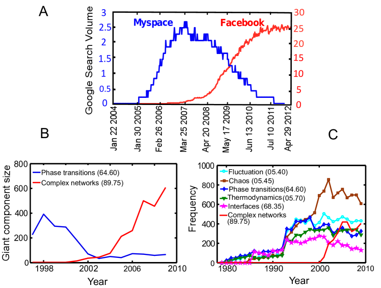
Figure 1:

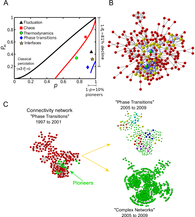
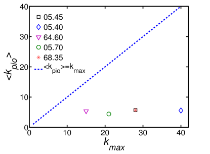
(D)

Figure 2:

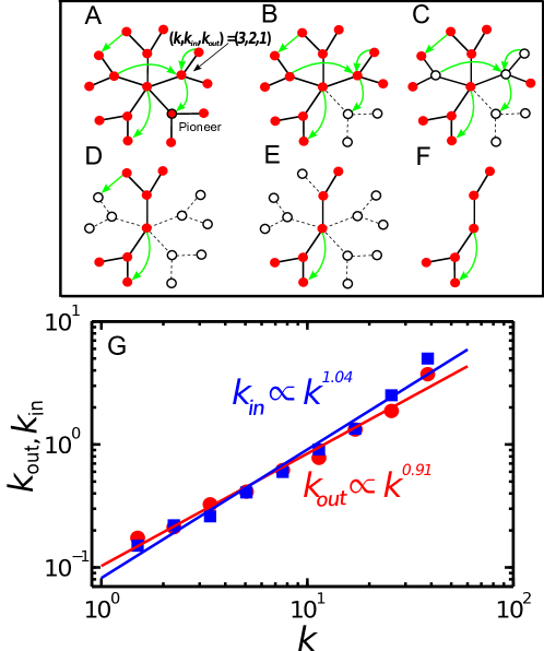
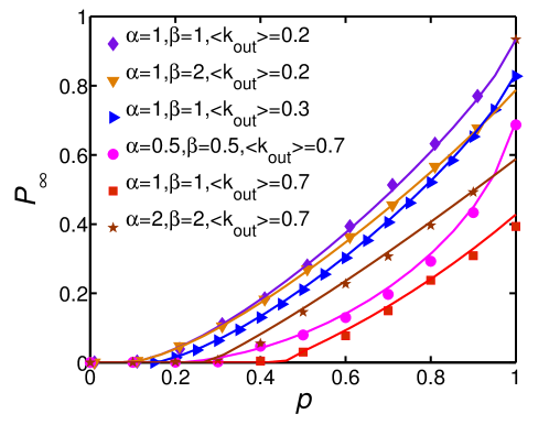
(H)

Figure 3:

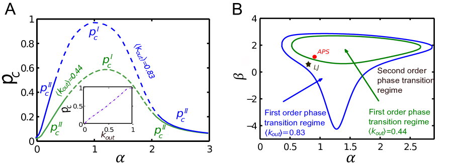
Figure 4:

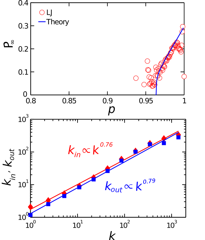
Figure 5:

SUPPLEMENTARY INFORMATION

Conditions for viral influence spreading through correlated multiplex networks

Yanqing Hu, Shlomo Havlin, Hernán A. Makse

IV General properties of studied networks

We consider the top five PACS numbers contributing scientists to the Complex Networks field. The PACS numbers are listed in Table 1. The whole dataset is made available at http://jamlab.org and it was provided by APS. The field of “Complex Networks” started in 2001 in the Physics community and encompasses a series of PACS numbers under the general class: 89.75, “Complex systems”. This generic PACS number contains the subclasses: 89.75.Da, “Systems obeying scaling laws”. 89.75.Fb, “Structures and organization in complex systems” 89.75.Hc, “Networks and genealogical trees”. The newly developed community of “Complex Networks” published under the above PACS numbers. To test this assumption we have checked all APS papers with PACS Number 89.75 from 2000 to 2009. We have checked that the titles of 1193 papers in PACS 89.75 contain at least one of these words: ‘”network”, “networks”, “graph”, “graphs”, “link”, “links” and “degree”. Then, it is reasonable to assume that this PACS number has been assimilated by the newly formed community of Complex Networks. Indeed, the present paper will be archived under PACS 89.75.

According to the record in the APS database, we find all the scientists who at least published one scientific paper with PACS number 89.75 from 2001 to 2009, then go back to the period 1993 to 2000 and count the frequency of all PACS number used by these scientists. Thus we can detect the order of each PACS number contributing to network science. The top five PACS numbers contributing to Complex Networks are (ordered from large to small):

1. 05.45. Nonlinear dynamics and chaos. Includes: Low-dimensional chaos, Fractals, Control of chaos, applications of chaos, Numerical simulations of chaotic systems, Time series analysis, Synchronization; coupled oscillators, etc.

2. 05.40. Fluctuation phenomena, random processes, noise, and Brownian motion. Includes: Noise, Random walks and Levy flights, Brownian motion.

3. 68.35. Solid surfaces and solid-solid interfaces. Include: Interface structure and roughness, Phase transitions and critical phenomena, Diffusion; interface formation, etc.

4. 64.60. General studies of phase transitions. Includes: Specific approaches applied to studies of phase transitions, Renormalization-group theory, Percolation, Fractal and multifractal systems, Cracks, sandpiles, avalanches, and earthquakes, General theory of phase transitions, Order-disorder transformations, Statistical mechanics of model systems, Dynamic critical phenomena, etc.

5. 05.70. Thermodynamics. Includes: Phase transitions: general studies, Critical point phenomena, Nonequilibrium and irreversible thermodynamics, Interface and surface thermodynamics.

Table 1: General properties of the APS communities according to their PACS numbers. Values are calculated for $s=2$. $N_{\infty}$ is the size of the largest connected component calculated from 1997 to 2001, $n_{\infty}$ is the size of the largest component from 2005 to 2009, $\langle k_{\rm pio}\rangle$ is the average connectivity degree of the departing pioneers in 2001, $k_{\rm max}$ is the maximum connectivity degree, $\langle k\rangle$ is the average connectivity degree.

Field	PACS	$N_{\infty}$	$n_{\infty}$	$\langle k\rangle$	$\langle k_{\rm pio}\rangle$	$k_{\rm max}$
1. Chaos	05.45	1126	846	4.26	5.56	40
2. Fluctuations	05.40	522	227	3.97	5.68	28
3. Interfaces	68.35	232	77	5.64	4.14	21
4. Phase transitions	64.60	193	36	3.84	5.69	28
5. Thermodynamics	05.70	87	32	3.70	5.36	15
Complex networks	89.75	9	190	-	-	-

For each APS network identified by the above PACS numbers, we calculate the size of the largest connected component $N_{\infty}$ using the coauthorship in papers published over a window of 5 years from 1997 to 2001 using the threshold $s=2$ (the results are similar with $s=1$ and $3$). That is, we consider scientists who published at least $s$ papers together from 1993 to 2009. Using the publication information of 2001 we detect the fraction $1-p$ of authors who published at least one paper in Complex Networks. We then use a new 5 years window to define a network from 2005 to 2009 for each PACS number, and calculate the new size of the largest component, $n_{\infty}$. In these five years, a scientist may publish papers with the given PACS number and 89.75 or both. In this case, we classify the paper into 89.75 when the scientist published with 89.75 more times than other PACS numbers during the five year period. Thus, we obtain the relative size of the largest component $P_{\infty}(p)=n_{\infty}/N_{\infty}$ for each PACS field, which represents a measurement of the probability that a randomly chosen node belongs to the spanning cluster in percolation theory. The calculation is performed for $s=2$ and is plotted in Fig. 2a (other values of $s$ yield similar results).

LiveJournal.com.– LiveJournal (LJ) is a large social network of 8,312,972 users who post information and articles of common interest. In LJ, each user maintains a friends list, which declares social links to these individuals. The network resulting from these social links is believed to reliably represent actual social relations of LJ users. This network represents the connectivity links in our model. More importantly, since we know the entire history of posts over several years, we can use this information to quantify the influence links between two users: if user $i$ cited repeatedly the posts of user $j$, then we consider an influence link from $i\to j$ since $i$ is a follower of $j$. In LJ, the communities are declared by the users, and users change interest very often, creating and disintegrating communities quite often. In the two years period when we recorded LJ, we find that there are 10,981 communities that are being disintegrated. We analyze only communities with more than 300 members, the largest of which contains almost half of LJ. We have the full data on the network connectivity and the influence connectivity of LJ from February 14th, 2010 to November 21st, 2011. To calculate the percolation plot $(p,P_{\rm infty})$ we consider the size of the giant component of a declining community at the beginning of the period of observation and compare with the size of the same community at the end of the observation window.

The communities in LiveJournal evolve at a much faster pace than the scientific communities in APS. Indeed, we need many years (the APS dataset spans 35 years) to see an idea to be established in the scientific community. Further, many scientists keep working in their old fields, while moving to a new one. However, the pace of change is much faster in an online blogging community like LJ. In LJ, the communities are declared by the users, and users change interest very often, creating and disintegrating communities quite often.

IV.1 General features in the dynamics of followers

Evidence of the cascading processes triggered by the pioneers is depicted in SI Fig. 6 showing general features in the dynamics of followers. We track the pioneers who first published in Complex Networks in 2001, then the followers and then the rest. For each of the top 5 PACS number with 89.75 together, we calculate the largest component of the coauthorship network according to the APS publication records from 1997 to 2001. Using this data, we detect the pioneers of network science and all of the followers of pioneers in this coauthorship network. SI Fig. 6 shows general features in the dynamics of followers. We compare the fraction of papers published in complex networks among pioneers, followers and the rest for different PACS number form 2001 to 2009 and found that the fraction satisfies that pioneers$>$followers$>$the rest. This suggests that influence links follows the influence links in a cascade of followers.

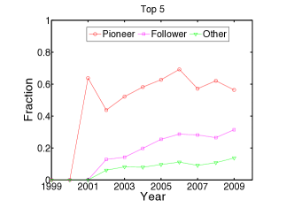
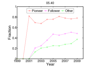
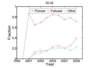
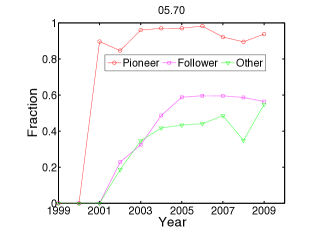
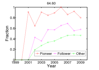
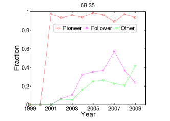
Figure 6: Comparison of the fraction of papers published by pioneers, followers and followers of followers. Followers are the scientists who at least cited one paper of the pioneers between 1997 to 2001 and are not the cooperators of pioneers. For a given PACS number as indicated in the figures, we record the number of papers published in the PACS number and the number of papers published only in 89.75 (Complex Networks) for each author. Then we get the total number of papers published in complex networks $N_{\rm net}$ and the number of papers with these two PACS numbers $N_{\rm all}$ for every author. The vertical axis shows the fraction $\frac{N_{\rm net}}{N_{\rm all}}$ as a function of time, which approximately satisfies pioneers$>$followers$>$the rest. This result suggests that influence links are important for cascading dynamics.

V Generating function theory of percolation in correlated influence networks

We consider a network with both, bidirectional connectivity links and directed influence links. Each node has three degrees: $(k,k_{\rm in},k_{\rm out})$ measuring the number of connectivity links, in-going influence links and out-going influence links, respectively. The properties of such a network are described by the three dimensional generating function:

$$G(x_{1},x_{2},x_{3})=\sum_{k,k_{\rm in},k_{\rm out}}P(k,k_{\rm in},k_{\rm out})x_{1}^{k}x_{2}^{k_{\rm in}}x_{3}^{k_{\rm out}},$$ (13)

where the joint probability distribution $P(k,k_{\rm in},k_{\rm out})$ describes the local correlations among $(k,k_{\rm in},k_{\rm out})$. In the following we denote the higher order derivatives as:

$$G_{x_{1}^{m_{1}},x_{2}^{m_{2}},x_{3}^{m_{3}}}(x_{1},x_{2},x_{3})=\frac{\partial^{m_{1}+m_{2}+m_{3}}G(x_{1},x_{2},x_{3})}{\partial x_{1}^{m_{1}}\partial x_{2}^{m_{2}}\partial x_{3}^{m_{3}}}.$$ (14)

If node $i$ is being influenced by node $j$, there is a directed influence link from node $i$ to node $j$. In a real system, the influence of the piers is applied with a given probability $q_{h}$ which is less than 1. That is, even if there is an influence link from $i$ to $j$, if $j$ departs, then $i$ will depart with probability $q_{h}$ which in general is smaller than 1. In SI Section X we explain in detail how to estimate $q_{h}$ from the APS data. This effect is taken into account in the model. In order to simplify the problem, the removal following influence links is analogous to randomly deleting a $1-q_{h}$ fraction of influence links, and then assuming that all of the remaining nodes connected via influence links are removed with probability 1. Without losing any generality, in our analysis we set this probability to be $q_{h}=1$, as done in previous percolation studies NewmanSpread . Next, we analyze the cascading process following the recursive stages: percolation process $\to$ influence-induced percolation process $\to$ percolation process $\to$ influence-induced percolation $\cdots$.

V.1 First Stage: Classical Percolation Process

The cascading process is triggered by initially randomly removing a fraction of $1-p$ nodes. We use $\tilde{p}$ to denote the fraction of remaining nodes after initial random removing. Thus, at this first stage, we have:

$$\tilde{p}=p.$$ (15)

The generating function of the connectivity degree distribution related to the branching process is $\frac{G_{x_{1}}(x_{1},1,1)}{G_{x_{1}}(1,1,1)}$Callaway ; PerLong ; sergey . Thus the giant component size $x$ after the first stage of the percolation process can be written as:

$$x=p[1-G(t,1,1)],$$ (16)

where,

$$t=1-\tilde{p}(1-f),$$ (17)

and

$$f=\frac{G_{x_{1}}(1-\tilde{p}(1-f),1,1)}{G_{x_{1}}(1,1,1)}.$$ (18)

The physical meaning of the quantity $t$ is that, a node with connectivity degree $k$ will have $1-t^{k}$ probability staying in the giant component SgPRE . Accordingly, we get the average in-degree in the giant component of size $x$, $\langle k_{\rm in}^{x}\rangle$, as:

$$\langle k_{\rm in}^{x}\rangle=\frac{G_{x_{2}}(1,1,1)-G_{x_{2}}(t,1,1)}{1-G(t,1,1)}.$$ (19)

V.2 Second Stage: Influence-Induced Percolation Process

In order to treat the local correlations between $(k,k_{\rm in},k_{\rm out})$, we develop a generating function theory for the first time by combining the percolation process on the connective links and the influence directed links in a correlated fashion. It is instructed to treat first the second stage assuming that the network has influence links but they are uncorrelated and then we will generalize the results to the existence of correlation.

Let $H(u)$ be the generating function for the probability of reaching an outgoing component of a given size by following a directed links on the original network. According to reference cohen , $H(u)$ can be written as

$$H(u)=u\frac{G_{x_{2}}(1,1,H(u))}{\langle k_{\rm in}\rangle}.$$ (20)

Let,

$$H(u)=\sum_{s}\eta(s)u^{s}.$$ (21)

Assuming we can reach $s$ nodes following an out-going directed link (influence links), thus for any given random subnetwork of size $u$ (randomly selected from the original network), the probability for all of the $s$ nodes to be in $u$ is $u^{s}$. This means that the generating function for the probability that all the nodes reached by following a directed link are in $u$ is $H(u)$.

Next, we generalize the above argument by considering a correlated selection of nodes in $u$, rather than considering a random uncorrelated selection of nodes in $u$ as above. If we choose the nodes in a correlated fashion with the in-degree $k_{\rm in}$ only, any local structure in $u$ are still tree like. Thus the probability that all the nodes reached by following a directed link are in $u$ is proportional to the sum of the in-degree of all nodes in $u$. Let

$$\hat{u}=\frac{\langle k_{\rm in}^{u}\rangle}{\langle k_{\rm in}\rangle},$$ (22)

then, the generating function of the probability that all the nodes reached by following a directed link are in $u$ is $H(\hat{u})$. Furthermore, a node with $k_{\rm out}$ degree in $u$ will survive with probability $H^{k_{\rm out}}(\hat{u})$.

Considering the directed network composed by influence links, the generating function of the out-degree distribution is $G(1,1,x_{3})$ and the corresponding generating function of the out-degree related to the directed branching process is $\frac{G_{x_{2}}(1,1,H(x))}{\langle k_{\rm in}\rangle}.$ Using $y$ to denote the probability that all the nodes reached by following a directed link are in $x$, we have

$$y=H(hx),$$ (23)

where,

$$H(x)=x\frac{G_{x_{2}}(1,1,H(x))}{\langle k_{\rm in}\rangle},$$ (24)

and

$$h=\frac{\langle k_{\rm in}^{x}\rangle}{\langle k_{\rm in}\rangle}.$$ (25)

V.3 Third Stage: Recursive Percolation Process

Removing a node with $k$ and $k_{\rm out}$ in the second stage is analogous to removing the node with probability $1-py^{k_{\rm out}}$ from the original network in the first stage. This crucial property implies that we can map out the cascading process after the second stage into a new initial removing occurring in the original network. The fraction of remaining links after the new removing process is:

$$\tilde{p}=\frac{pG_{x_{1}}(1,1,y)}{G_{x_{1}}(1,1,1)}.$$ (26)

Thus, the resulting percolation equations are

$$f=\frac{G_{x_{1}}[1-\tilde{p}(1-f),1,y]}{G_{x_{1}}(1,1,y)},$$

$$t=1-\tilde{p}(1-f),$$

$$x=p[1-G(t,1,1)].$$

V.4 Recursive relations

The above analysis leads to a set of recurring relations defining the cascading process. After the second stage, the current cascading effect can be mapped to a removing process in the original network. This property allows us to write down the cascading process as recursive equations. Integrating the above three stages, we can rewrite the cascading process as following:

$$x=p[1-G(1-\tilde{p}(1-f),1,1)],$$ (28)

$$f=\frac{G{x_{1}}(1-\tilde{p}(1-f),1,y)}{G_{x_{1}}(1,1,y)},$$

$$\tilde{p}=\frac{pG_{x_{1}}(1,1,y)}{G_{x_{1}}(1,1,1)},$$

$$t=1-\tilde{p}(1-f),$$

$$\langle k_{\rm in}^{x}\rangle=\frac{G_{x_{2}}(1,1,1)-G_{x_{2}}(t,1,1)}{1-G(t,1,1)},$$

$$h=\frac{\langle k_{\rm in}^{x}\rangle}{\langle k_{\rm in}\rangle},$$

$$y=hx\frac{G_{x_{2}}(1,1,y)}{\langle k_{\rm in}\rangle}.$$

The physical meaning of these recursion relations is that, after each first stage, a node that is not removed in the initial attack has $1-t^{k}$ survival probability. After the second stage, the survival node can be mapped out to a removing process occurring on the original network with probability $1-py^{k_{\rm out}}$. These two properties allow us to write down the formula of the relative size of giant component $P_{\infty}$ at the final stable state of the cascading process as:

$$P_{\infty}(p)=p[G(1,1,y)-G(t,1,y)].$$ (29)

VI The critical threshold and universal boundary for phase transitions

It is of interest to understand the universal properties at the critical point. Below we derive the critical threshold for first-order and second-order transitions, and the boundaries between these two phases. The equations are valid for any type of correlations. In the following sections we apply our results to uncorrelated and correlated networks with influence links.

VI.1 Second-order phase transition

When the transition is of second order, the giant component $P_{\infty}$ tends to 0 continuously as $p$ approaches the critical threshold $p_{c}^{\rm II}$. This implies that when $p\rightarrow p_{c}^{\rm II}$, $x\rightarrow 0$ and $y\rightarrow 0$, as well as $t\rightarrow 1$ and $f\rightarrow 1$, continuously. Let

$$z=\tilde{p}(1-f),$$ (30)

and the second equation of the main recursive Eqs. (28) can be written as

$$f=\frac{\sum_{k,k_{\rm in},k_{\rm out}}P(k,k_{\rm in},k_{\rm out})k(1-z)^{k-1}y^{k_{\rm out}}}{\sum_{k,k_{\rm in},k_{\rm out}}P(k,k_{\rm in},k_{\rm out})ky^{k_{\rm out}}}.$$ (31)

Thus,

$$f=\frac{\sum_{k,k_{\rm in},k_{\rm out}}P(k,k_{\rm in},k_{\rm out})k\sum_{\mu=0}^{k-1}C^{k-1}_{\mu}(-z)^{\mu}y^{k_{\rm out}}}{\sum_{k,k_{\rm in},k_{\rm out}}P(k,k_{\rm in},k_{\rm out})ky^{k_{\rm out}}},$$ (32)

When $p\rightarrow p_{c}^{\rm II}$, then $z\rightarrow 0$. Therefore, close to the critical point we can ignore the terms of order $O(z^{2})$ and $O(y)$, and the above equation can be written as:

$$f=\frac{\sum_{k,k_{\rm in},0}P(k,k_{\rm in},0)[k-k(k-1)z+\frac{1}{2}k(k-1)(k-2)z^{2}]+\sum_{k,k_{\rm in},1}P(k,k_{\rm in},1)[ky-k(k-1)zy+\frac{1}{2}k(k-1)(k-2)z^{2}y]}{\sum_{k,k_{\rm in},0}P(k,k_{\rm in},0)k+\sum_{k,k_{\rm in},1}P(k,k_{\rm in},1)ky}.$$ (33)

Using Eq. (30), Eq. (33) can be reduced to:

$$z=\frac{\sum_{k,k_{\rm in},0}P(k,k_{\rm in},0)[k(k-1)-\frac{1}{\tilde{p}}k]+\sum_{k,k_{\rm in},1}P(k,k_{\rm in},1)[k(k-1)y-\frac{1}{\tilde{p}}ky]}{\sum_{k,k_{\rm in},0}P(k,k_{\rm in},0)\frac{1}{2}k(k-1)(k-2)+\sum_{k,k_{\rm in},1}P(k,k_{\rm in},1)\frac{1}{2}k(k-1)(k-2)y}.$$ (34)

Using the forth equation in the main system Eqs. (28), we obtain:

$$t=t(y)=1-\frac{\sum_{k,k_{\rm in},0}P(k,k_{\rm in},0)[k(k-1)-\frac{1}{\tilde{p}}k]+\sum_{k,k_{\rm in},1}P(k,k_{\rm in},1)[k(k-1)y-\frac{1}{\tilde{p}}ky]}{\sum_{k,k_{\rm in},0}P(k,k_{\rm in},0)\frac{1}{2}k(k-1)(k-2)+\sum_{k,k_{\rm in},1}P(k,k_{\rm in},1)\frac{1}{2}k(k-1)(k-2)y}.$$ (35)

Note that, here, $t$ is written as a function of $y$.

When $y\to 0$, the 7th equation of the main system Eqs. (28) can be written as

$$y=y(t)=hx\frac{\sum_{k,k_{\rm in},0}P(k,k_{\rm in},0)k_{\rm in}}{\langle k_{\rm in}\rangle}.$$ (36)

Substituting Eqs. (28) into Eq. (36), we obtain:

$$y(t)=\frac{G_{x_{2}}(1,1,1)-G_{x_{2}}(t,1,1)}{\langle k_{\rm in}\rangle[1-G(t,1,1)]}\cdot\frac{p[1-G(t,1,1)]\frac{1}{\langle k_{\rm in}\rangle}\sum_{k,k_{\rm in},0}P(k,k_{\rm in},0)k_{\rm in}}{1-\sum_{k,k_{\rm in},1}P(k,k_{\rm in},1)k_{\rm in}}.$$ (37)

Note that, here we write $y$ as a function of $t$.

By simplifying the third equation of the main system (28), we obtain:

$$\tilde{p}=\frac{p\sum_{0,k_{\rm in},k_{\rm out}}p(0,k_{\rm in},k_{\rm out})k}{\langle k\rangle}.$$ (38)

Substituting Eqs. (35) and (38) into Eq. (37) and ignoring terms of higher order in $y$, we obtain the explicit formula for the critical point in the second order phase transition:

$$p_{c}^{\rm II}=\frac{\langle k\rangle}{G_{x_{1}^{2}}(1,1,0)}.$$ (39)

This equation generalizes the classical uncorrelated percolation result for networks without influence links, $p_{c}=\frac{\langle k\rangle}{\langle k(k-1)\rangle}$ cohena ; satorras01 ; barabasi-attack ; NewmanSpread ; Callaway to an influence network with generic correlations, $P(k,k_{\rm in},k_{\rm out})$.

VI.2 First-order phase transition

For a given $G(x_{1},x_{2},x_{3})$, if there exist a first-order phase transition, the critical point function $t(y)$, Eq. (35) and $y(t)$ Eq. (37) must be tangential to each other (as shown in SI Fig. 7). Thus, the condition for a first-order phase transition is

$$\frac{\partial t(y,p_{c}^{\rm I})}{\partial y}\big{|}_{y=0}\cdot\frac{\partial y(t,p_{c}^{\rm I})}{\partial t}\big{|}_{t=1}=1.$$ (40)

Contrary to the case of $p_{c}^{\rm II}$ in Eq. (39), it is usually not possible to find an explicit formula for $p_{c}^{\rm I}$ from Eq. (40). Therefore, we resort to a numerical integration of Eq. (40).

Figure 7: Condition for a first-order phase transition. This figure shows that the functions $t(y)$ and $y(t)$ are tangential at the critical point when the transition is of the first order. Here $\langle k_{\rm out}\rangle=0.74$, $\gamma=3$ and minimum degree $m=2$.

VI.3 Boundary between transitions

According to Eq. (35), (38) and (39), we obtain:

$$\frac{\partial t}{\partial y}\big{|}_{y=0}=-\frac{\sum_{k,k_{\rm in},1}P(k,k_{\rm in},1)\Big{[}k(k-1)-\frac{G_{x_{1}}(1,1,1)}{p_{c}^{\rm I}G_{x_{1}}(1,1,0)}k\Big{]}-\frac{p_{c}^{\rm I}G_{x_{1},x_{3}}(1,1,0)G_{x_{1}}(1,1,1)}{[p_{c}^{\rm I}G_{x_{1}}(1,1,0)]^{2}}\sum_{k,k_{\rm in},0}P(k,k_{\rm in},0)k}{\frac{1}{2}\sum_{k,k_{\rm in},0}P(k,k_{\rm in},0)k(k-1)(k-2)},$$ (41)

and

$$\frac{\partial y}{\partial t}\big{|}_{t=1}=\frac{-G_{x_{1},x_{2}}(1,1,1)p_{c}^{\rm I}G_{x_{2}}(1,1,0)}{\langle k_{\rm in}\rangle^{2}}.$$ (42)

Substituting Eqs. (41) and (42) into Eq. (40) we obtain the boundary between the first and second order phase transitions regime in the phase space:

$$1=\frac{2p_{c}^{\rm II}\langle k\rangle G_{x_{1}^{2},x_{3}}(1,1,0)hG_{x_{2}}(1,1,0)}{\langle k_{\rm in}\rangle G_{x_{1}^{3}}(1,1,0)}.$$ (43)

There also exists an additional boundary between a stable network and unstable network with $p_{c}=1$. Such a network will disintegrate after removing a vanishing fraction of nodes in the thermodynamic limit.

VII Networks with uncorrelated influence links

We treat the case of a random uncorrelated network with influence links but no local correlations among $(k,k_{\rm in},k_{\rm out})$. In this case $h\equiv 1$, and the main system (28) can be reduced to:

$$x=p[1-G(1-\tilde{p}(1-f),1,1)],$$ (44)

$$f=\frac{G{x_{1}}(1-\tilde{p}(1-f),1,y)}{G_{x_{1}}(1,1,y)},$$

$$\tilde{p}=\frac{pG_{x_{1}}(1,1,y)}{G_{x_{1}}(1,1,1)},$$

$$t=1-\tilde{p}(1-f),$$

$$y=x\frac{G_{x_{2}}(1,1,y)}{\langle k_{\rm in}\rangle}.$$

$$P_{\infty}=p[G(1,1,y)-G(t,1,y)].$$

Simplifying the above system, at the equilibrium state the giant component $P_{\infty}$ can be written as:

$$P_{\infty}=pG(1,1,P_{\infty})\{1-G[1-pG(1,1,P_{\infty})(1-f),1,1]\},$$ (45)

and

$$f=\frac{G_{x}[1-pG(1,1,P_{\infty},1,1)(1-f)]}{G_{x}(1,1,1)}.$$ (46)

When the transition is second order, the critical point can be obtained explicitly as:

$$p_{c}^{\rm II,unc}=\frac{\langle k\rangle}{q_{0}\langle k(k-1)\rangle},$$ (47)

where, $q_{0}$ is the fraction of nodes with $k_{out}=0$. Therefore, for a scale-free network with $\gamma<3$, we find $p_{c}^{\rm II,unc}=0$, since the second moment diverge, despite the presence of the influence links, as long as these links are uncorrelated with each other.

VIII Networks with correlated influence links

When $k_{in}$ and $k_{out}$ correlate with $k$, the generating function $G(x_{1},x_{2},x_{3})$ can be written as:

$$G(x_{1},x_{2},x_{3})=\sum_{k}P_{1}(k)x_{1}^{k}\cdot\sum_{k_{in}}P_{2}(k_{in}|k)x_{2}^{k_{in}}\cdot\sum_{k_{out}}P_{2}(k_{out}|k)x_{2}^{k_{out}}.$$ (48)

For a given $P_{1}(k)$ and $(\alpha,\beta,\langle k_{\rm in}\rangle)$, the average in-degree and out-degree for given $k$ are $\frac{k^{\beta}}{\langle k^{\beta}\rangle}\langle k_{\rm in}\rangle$, where $\langle k^{\alpha}\rangle=\sum_{k}P_{1}(k)k^{\alpha}$ and $\langle k^{\beta}\rangle=\sum_{k}P_{1}(k)k^{\beta}$. $P_{2}(k_{\rm in}|k)$, $P_{3}(k_{\rm out}|k)$ is assumed to be both Poisson distributions (see SI Fig. 8), thus the generating functions for $P_{2}(k_{\rm in}|k)$ and $P_{3}(k_{\rm out}|k)$ are $\sum_{k_{in}}P_{2}(k_{in}|k)x_{2}^{k_{in}}=e^{\frac{1}{\langle k^{\beta}\rangle}\langle k_{\rm in}\rangle k^{\beta}(x_{2}-1)}$ and $\sum_{k_{out}}P_{2}(k_{out}|k)x_{2}^{k_{out}}=e^{\frac{1}{\langle k^{\alpha}\rangle}\langle k_{\rm in}\rangle k^{\alpha}(x_{3}-1)}$. Therefore, the main generating function can be written as:

$$G(x_{1},x_{2},x_{3})=\sum_{k}P_{1}(k)x_{1}^{k}e^{\frac{1}{\langle k^{\beta}\rangle}\langle k_{\rm in}\rangle k^{\beta}(x_{2}-1)}e^{\frac{1}{\langle k^{\alpha}\rangle}\langle k_{\rm in}\rangle k^{\alpha}(x_{3}-1)}.$$ (49)

This simple formula allow us to solve for $p_{c}^{\rm II}$ for any $\alpha$ and $\beta$. Using Eq. (49), we can write the critical threshold as:

$$p_{c}^{\rm II,cor}=\frac{\langle k\rangle}{\sum_{k}k(k-1)P(k)\exp\Big{(}{\frac{-k^{\alpha}\langle k_{\rm in}\rangle}{\langle k^{\alpha}\rangle}\Big{)}}}.$$ (50)

When there is no local correlation between $k$ and $k_{\rm out}$, $\alpha=0$ and $\exp\Big{(}{\frac{-k^{\alpha}\langle k_{\rm out}\rangle}{\langle k^{\alpha}\rangle}}\Big{)}=\exp\Big{(}-\langle k_{\rm out}\rangle\Big{)}=q_{0}$ which is consistent with the uncorrelated result Eq. (10).

Equation (50) indicates that $p_{c}^{\rm II,cor}$ only depends on $\alpha$, the connectivity degree distribution $P(k)$ ($\gamma$ in the case of a scale-free network) and the average in-degree or out-degree since $\langle k_{\rm in}\rangle=\langle k_{\rm out}\rangle$. Furthermore, $p_{c}^{\rm II,cor}$ can be different from zero even for a scale-free network with $\gamma<3$— unlike the uncorrelated counterpart, Eq. (47)— since the exponential term stabilizes the divergence of the second moment when $\alpha\neq 0$. Surprisingly, there is no $\beta$ dependence, implying that the large correlation between $k$ and $k_{\rm in}$ plays a secondary role in sustaining the cascades or in changing $p_{c}^{\rm II,cor}$. When the transition is of the first order, $p_{c}^{\rm I,cor}$ depends on both $\alpha$ and $\beta$.

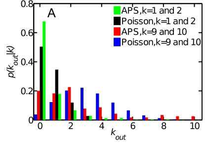
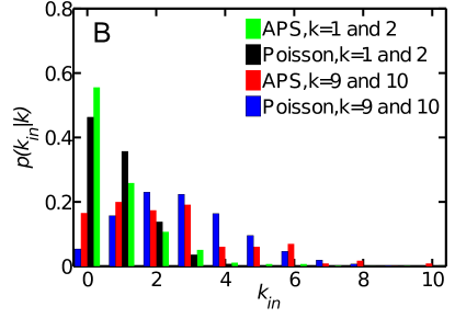
Figure 8: Distribution of (a) $P(k_{\rm out}|k)$ and (b) $P(k_{\rm in}|k)$ for the five APS communities. We calculate the probability of $k_{\rm in}$ and $k_{\rm out}$ for a given $k$ and find that they can be approximated by Poisson distributions.

IX Estimation of distribution functions based on exponential random graph models

Exponential-family random graph models ERGMWasserman1 are very useful statistical tools to capture the essential properties of networks. Here, we employ this tool to estimate the power law exponent of the degree distribution. For the exponential-family models, we define

$$P_{\theta}(\Omega=\omega)=\exp\Big{[}\sum_{k=0}^{n}\theta_{k}p_{k}(\omega)\Big{]},$$ (51)

where $p_{k}(\omega)$ is the probability of randomly choosing a node with degree $k$ in network $\omega$. We use conditional logistic regression method to estimate the full vector $\theta$. It is a pseudo-likelihood method Hunter which estimate the vector $\theta$ by maximizing

$$l(\theta)=\sum_{i,j}\Big{[}P_{\theta}\big{(}\Omega_{i,j}=\omega_{i,j}\big{|}\Omega_{u,v}=\omega_{u,v},(u,v)\neq(i,j)\big{)}\Big{]}.$$ (52)

After obtaining the vector $\theta$, we employ the Gibbs sampling to update the links of the network. For a given initial network $\omega^{1}$ (step 1), the links of this network are stochastically updated. In step $t$, the probability of the existence of the link between node $i$ and $j$ is

$$P_{\theta}\Big{(}\omega_{i,j}^{t+1}=1\big{|}\omega_{u,v}^{t+1}=\omega_{u,v}^{t},(u,v)\neq(i,j)\Big{)}.$$ (53)

The distribution of the network $\omega^{t}$ converges for $t\to\infty$ to the exponential random graph distribution. The above updating process is so-called Markov chain Monte Carlo (MCMC) Hunter . In this way, we can get a lot of network samples and the corresponding degree sequences. It allows us to estimate the power law exponent of the original networks by bootstrap method. We employ the standard maximum likelihood methods maxlikehood to estimated the power law exponent of degree distribution for each networks and get the average value and standard deviation of this exponent is $\gamma=2.9\pm 0.01.$

X Estimation of the average number of influence links

First, we detect all the pioneers who have published at least one Complex Network paper in 2001 and then find all authors who have cited this pioneers (the followers). Then we identify which followers have published a paper in Complex Networks in 2002-2003. We use this information to estimate, from the real data, the maximum fraction of influence links for each number of citations $w$, as shown in SI Fig. 9. The lower and upper bounds of the averages $\langle k_{\rm out}\rangle(=\langle k_{\rm in}\rangle)$ are estimated from the interval $[\frac{\sum_{w}n_{w}f^{\rm min}_{w}}{N},\frac{\sum_{w}n_{w}f^{rmmax}_{w}}{N}],$ where $n_{w}$ is the number of influence links with weight $w$ in the giant component, $N$ is the size of the giant component and $f^{\rm min}_{w}$, $f^{\rm max}_{w}$ are the minimum and maximum active influence links estimated as follows.

To calculate $f^{\rm max}_{w}$, we consider the number of authors that cite a given author and calculate the number of influence links which are active as those from a follower who actually leave the network: $f^{\rm max}_{w}=\frac{a^{\rm max}_{w}}{A_{w}}$ and $f^{\rm min}_{w}=\frac{a^{\rm min}_{w}}{A_{w}}$, where $a^{\rm max}_{w}$ and $a^{\rm min}_{w}$ are the maximum and minimum number of active influence links with weight $w$, and $A_{w}$ is the number of links from the followers to the pioneers including both active and inactive links with weights $w$. For the calculation of $f^{\rm min}_{w}$, if a follower who moves to Complex Networks depends on several pioneers, we consider the influence link with the largest weight. SI Figure 9 illustrates the calculation with an example. Applying this calculation to the APS communities we find the lower and upper bounds of the average influence links as $\langle k_{\rm out}\rangle\in[0.44,0.83]$. The lower bound $\langle k_{\rm out}\rangle=0.44$ is used to calculate $P_{\infty}(p)$ in Fig. 2a, which shows how all the empirical data is between the estimated bounds.

To measure the correlations between connectivity degree and in- and out-degree, first, we employ the above method to measure the influence probability for each directed influence link for a given network. Different weights of the directed links gives rise to different probabilities. We keep the directed links with these probability and record all pairs $(k,k_{out})$, $(k,k_{in})$. We repeat this calculation 20 times and compute the average in- and out-degree for all the node whose connectivity degree is $k$. Using the pairs $(k,k_{\rm out})$ and $(k,k_{\rm in})$, the correlation scaling law of Fig. 2d can be obtained.

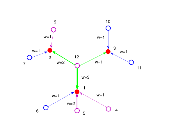
Figure 9: Estimation of $f^{\rm min}_{w}$ and $f^{\rm max}_{w}$ to obtain the bounds in $\langle k_{\rm out}\rangle$ from the empirical data. In the figure, we show three pioneers (red nodes), citation links with weights $w$ given by the number of citations, and all of the followers of the pioneers (open circle). The purple open circles denote the followers who move to Complex Networks, while the blue open circles do not move. For the calculating of $f^{max}_{w}$, we consider the links that are active as those from followers who move to Complex Networks. In the figure, all the green and purple directed links are active. We estimate $f^{\rm max}_{w}=\frac{a^{\rm max}_{w}}{A_{w}}$ and $f^{\rm min}_{w}=\frac{a^{\rm min}_{w}}{A_{w}}$ as indicated in the text. For the calculation of $f^{\rm min}_{w}$, if a follower who moves to Complex Networks depends on several pioneers, we consider the influence link with the largest weight. For instance, for all the green influence links in the figure, the links from node 12 to 1 with weight 3 is active and the links from 12 to 2 and 3 are not active. In this case we obtain: $f^{\rm max}_{1}=\frac{3}{7},f^{\rm max}_{2}=\frac{2}{2}=1,f^{\rm max}_{3}=1$, and $f^{\rm min}_{1}=\frac{2}{7},f^{\rm min}_{2}=\frac{1}{2},f^{\rm min}_{3}=1.$

XI Test of correlations between the connectivity and influence networks

We investigate the correlations between both networks by measuring the average influence degree (in and out) of the nearest neighbors, $\langle k_{\rm nn}\rangle$, of a node with connectivity degree $k$ connected via an influence link.

For the nodes with degree $k$, we measure the average degree $\langle k_{\rm nn}\rangle$ of their following and follower nodes. We find that there is almost no correlations between $\langle k_{\rm nn}\rangle$ and $k$ as shown in Fig. 10. The lack of correlations is indicated by a flat curve in the plot. We note that due to the fact that the degree distribution is power-law, the second moment is very broad, so that it makes the error bars (standard deviation) very large.

This result implies that the correlation between the connectivity networks and influence networks themselves are not significant in the APS, such that the present theory may suffice to capture the cascading effect. However, the correlations between both networks might become significant in other networks. In this case, the theory can be modified to incorporate these type of correlations. In such a case, the generating function should be generalized to a six-dimensional function as follows:

$$G(x_{1},x_{2},x_{3},x_{4},x_{5},x_{6})=\sum P(k^{1},k^{1}_{in},k^{1}_{out},k^{2},k^{2}_{in},k^{2}_{out})x_{1}^{k^{1}}x_{2}^{k^{1}_{in}}x_{3}^{k^{1}_{out}}x_{4}^{k^{2}}x_{5}^{k^{2}_{in}}x_{6}^{k^{2}_{out}}$$ (54)

to describe the coupled network system. Such a system will not be difficult to solve with the same techniques developed so far. The percolation techniques for a degree-correlated network would be analogous to those described in the works of Boguna M, Pastor-Satorras R, Vespignani A. (2003) Absence of epidemic threshold in scale-free networks with degree correlations. Phys. Rev. Lett. 90, 028701; and Goltsev AV, Dorogovtsev SN, Mendes JFF (2008) Percolation on correlated networks. Phys. Rev. E 78, 051105.

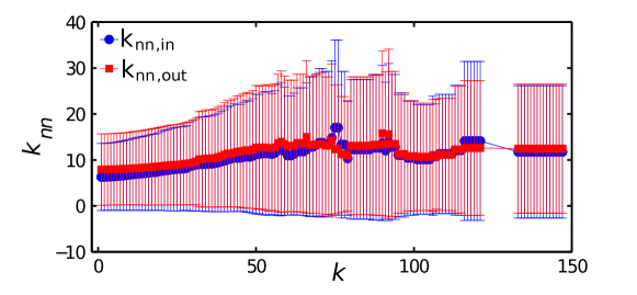
Figure 10: Correlations between connectivity and influence networks. A flat line indicates no correlations in the APS networks for $\langle k_{\rm nn}\rangle$ for the in-degree and $\langle k_{\rm nn}\rangle$ for the out-degree. In the degree sequence, there are no nodes with degree around $k=130$.

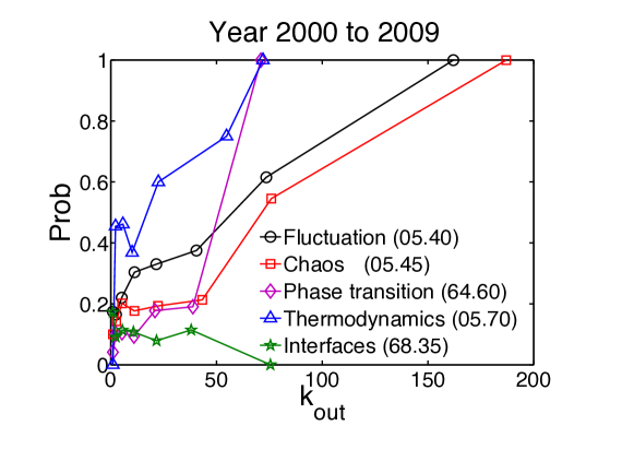
Figure 11: We measured the departure probability of nodes as a function of $k$ and $k_{\rm out}$ (number of followee). We observe that the hubs with larger number of cooperators $k$ and that are influenced by more scientists (larger $k_{\rm out}$) will move into a new field with larger probability.

References

- (1) T. C. Schelling, Micromotives and Macrobehavior (Norton) (1978).
- (2) G. Caldarelli, Scale-Free Networks: Complex Webs in Nature and Technology (Oxford Finance, 2007).
- (3) C. Castellano, S. Fortunato and V. Loreto, Statistical physics of social dynamics, Rev. Mod. Phys. 81, 591 (2009).
- (4) M. E. J. Newman, Networks: An Introduction (Oxford University Press, 2010).
- (5) E. Rogers, Diffusion of Innovations (Free Press, fourth edition, 1995).
- (6) T. W. Valente, Network Models of the Diffusion of Innovations (Hampton Press, Cresskill, NJ, 1995).
- (7) M. Granovetter, American Journal of Sociology 83, 1420 (1978).
- (8) D. J. Watts, A simple model of global cascades on random networks, Proc. Natl. Acad. Sci. USA. 99, 5766 (2002).
- (9) D. Kempe, J. Kleinberg and E. Tardos, Maximizing the spread of influence through a social network, in Proc. 9th ACM SIGKDD Intl. Conf. on Knowledge Discovery and Data Mining, Washington, DC (2003).
- (10) S. V. Buldyrev, R. Parshani, G. Paul, H. E. Stanley and S. Havlin, Catastrophic cascade of failures in interdependent networks, Nature 464, 1025 (2010).
- (11) P. Singh, S. Sreenivasan, B. K. Szymanski and G. Korniss, Threshold-limited spreading in social networks with multiple initiators, Sci. Rep. 3, 2330 (2013).
- (12) R. Parshani, S. V. Buldyrev and S. Havlin, Critical effect of dependency groups on the function of networks, Proc. Natl. Acad. Sci. U. S. A. 108, 1007 (2011).
- (13) M. Kurant and P. Thiran, Layered Complex Networks, Phys. Rev. Lett. 96, 138701 (2006).
- (14) P. J. Mucha, T. Richardson, K. Macon, M. A. Porter and J.-P. Onnela, Community structure in time-dependent, multiscale, and multiplex networks, Science 328, 876 (2010).
- (15) M. Szell, R. Lambiotte and S. Thurner, Multi-relational organization of large-scale social networks in an online world, Proc. Natl. Acad. Sci. U.S.A. 107, 13636 (2010).
- (16) R. G. Morris and M. Barthelemy, Transport on coupled spatial networks, Phys. Rev. Lett. 109, 128703 (2012).
- (17) S. Gómez, A. Díaz-Guilera, J. Gómez-Gardeñes, C. J. Pérez-Vicente, Y. Moreno and A. Arenas, Diffusion dynamics on multiplex networks, Phys. Rev. Lett. 110, 028701 (2013).
- (18) L.-L. Jiang and M. Perc, Spreading of cooperative behavior across interdependent groups, Sci. Rep. 3, 2483 (2013).
- (19) J. Nagler, A. Levina and M. Timme, Impact of single links in competitive percolation, Nature Phys. 7, 265 (2011).
- (20) X. Sun, J. Lei, M. Perc, J. Kurths and G. Chen, Burst synchronization transitions in a neuronal network of subnetworks, Chaos 21, 016110 (2011).
- (21) Z. Wang, A. Szolnoki and M. Perc, Interdependent network reciprocity in evolutionary games, Sci. Rep. 3, 1183 (2013).
- (22) M. Boguñá, M. A. Serrano, Generalized percolation in random directed networks, Phys. Rev. E 72, 016106 (2005).
- (23) G. J. Baxter, S. N. Dorogovtsev, A. V. Goltsev and J. F. F. Mendes, Avalanche collapse of interdependent networks, Phys. Rev. Lett. 109, 248701 (2012).
- (24) S.-W. Son, G. Bizhani, C. Christensen, P. Grassberger and M. Paczuski, Percolation theory on interdependent networks based on epidemic spreading, Europhys. Lett. 97, 16006 (2012).
- (25) M. E. J. Newman, Scientific collaboration networks. II. Shortest paths, weighted networks, and centrality, Phys. Rev. E 64, 016131 (2001).
- (26) L. Muchnik, S. Pei, L. C. Parra, S. D. Reis, Jr J. S. Andrade, S. Havlin and H. A. Makse, Origins of power-law degree distribution in the heterogeneity of human activity in social networks, Sci. Rep. 3, 1783 (2013), doi:10.1038/srep01783
- (27) L. K. Gallos, D. Rybski, F. Liljeros, S. Havlin and H. A. Makse, How people interact in evolving online affiliation networks, Phys. Rev. X 2, 031014 (2012).
- (28) D. S. Callaway, M. E. J. Newman, S. H. Strogatz and D. J. Watts, Network robustness and fragility: Percolation on random graphs, Phys. Rev. Lett. 85, 5468 (2000).
- (29) R. Cohen, K. Erez, D. ben-Avraham and S. Havlin, Resilience of the internet to random breakdowns, Phys. Rev. Lett. 85, 4626 (2000).
- (30) R. Albert, H. Jeong and A.-L. Barabási, Error and attack tolerance in complex networks, Nature 406, 378 (2000).
- (31) R. Pastor-Satorras and A. Vespignani, Epidemic spreading in scale-free networks, Phys. Rev. Lett. 86, 3200 (2001).
- (32) M. E. J. Newman, Spread of epidemic disease on networks, Phys. Rev. E 66, 016128 (2002).
- (33) M. E. J. Newman, S. H. Strogatz and D. J. Watts, Random graphs with arbitrary degree distributions and their applications, Phys. Rev. E 64, 026118 (2001) .
- (34) A. Clauset, C. R. Shalizi and M. E. J. Newman, Power-law distributions in empirical data, SIAM Rev. 51, 661 (2010).
- (35) http://www.google.com/trends/
- (36) S. V. Buldyrev, N. W. Shere and G. A. Cwilich, Interdependent networks with identical degrees of mutually dependent nodes, Phys. Rev. E 83, 016112 (2011).
- (37) N. Schwartz, R. Cohen, D. ben-Avraham, A.-L. Barabási and S. Havlin, Percolation in directed scale-free networks, Phys. Rev. E 66, 015104 (2002).
- (38) H. D. Rozenfeld, L. K. Gallos and H. A. Makse, Explosive percolation in the human protein homology network, Eur. Phys. J. B 75, 305 (2010).
- (39) M. E. J. Newman, Random graphs with clustering, Phys. Rev. Lett. 103, 058701 (2009).
- (40) S. S. Wasserman and P. Pattison, Logit Models and Logistic Regressions for Social Networks: I. An Introduction to Markov Graphs and p∗, Psychometrika 61, 401 (1996).
- (41) D. R. Hunter, M. S. Handcock, C. T. Butts, S. M. Goodreau and M. Morris, “ergm”: A Package to Fit, Simulate and Diagnose Exponential-Family Models for Networks, J. Statistical Software, 24, 1 (2008).