The wronskian solution of the constrained discrete KP hierarchy

Abstract.

From the constrained discrete KP (cdKP) hierarchy, the Ablowitz-Ladik lattice has been derived. By means of the gauge transformation, the Wronskian solution of the Ablowitz-Ladik lattice have been given. The $u_{1}$ of the cdKP hierarchy is a Y-type soliton solution for odd times of the gauge transformation, but it becomes a dark-bright soliton solution for even times of the gauge transformation. The role of the discrete variable $n$ in the profile of the $u_{1}$ is discussed.

Keywords: Constrained discrete KP hierarchy, Gauge transformation, Wronskian solution

Mathematics Subject Classification (2000): 37K10, 37K40, 35Q51, 35Q55.

1. Introduction

In the past few years, lots of attention have been given to the study of Kadomtsev-Petviashvili (KP) hierarchy [1, 2] in the field of integrable systems. The Lax pairs, Hamiltonian structures, symmetries and conservation laws, the $N$-soliton, tau function, the gauge transformation, reductions etc. of the KP hierarchy and its sub-hierarchies have been discussed. There are several sub-hierarchies of the KP by considering different reduction conditions on the Lax operator $L$. One of them is called constrained KP (cKP) hierarchy [3, 4, 5] by setting the Lax operator as $L=\partial+\sum_{i=1}^{m}\Phi_{i}\partial^{-i}\Psi_{i}$. The cKP hierarchy contains a large number of interesting soliton equations. The basic idea of this procedure is so-called symmetry constraint [3, 4, 5]. The negative part of the Lax operator of the constrained KP, i.e. $\sum_{i=1}^{m}\Phi_{i}\partial^{-i}\Psi_{i}$, is a generator [2] of the additional symmetry [6] of the KP hierarchy. And the additional symmetry of BKP hierarchy and CKP hierarchy have been given [7, 8]. Very recently, by a further modification of the additional flows, the additional symmetries of the constrained BKP and constrained CKP hierarchies are given in references [9, 10].

It is well known that a continuous integrable system has a discrete analogue in general. The famous 3-dimensional difference equation is known to provide a canonical integrable discretization for most important types of soliton equations. There are several different kinds of the discrete hierarchies including differential-difference KP (dKP) hierarchy [11, 12], semi-discrete integrable systems, full discrete equations and so on. The differential-difference KP hierarchy, defined by the difference operator $\Delta$, is one interesting object of the discrete integrable systems. Note that, the additional symmetry of dKP hierarchy and it’s Sato Bäcklund transformations have been given in reference [13]. Moreover, gauge transformation is one kind of powerful method to construct the solutions of the integrable systems for both the continuous KP hierarchy [14, 15, 16, 17, 18, 19, 20, 21, 22] and the dKP hierarchy [23, 24]. It is discussed to reduce the gauge transformation of the dKP hierarchy to the constrained discrete KP(cdKP) hierarchy [25]. And the algebraic structure of the additional symmetry of the cdKP hierarchy also has been found [26], which is same for the cKP hierarchy [8].

A crucial observation [12] about the KP hierarchy and the dKP hierarchy is that the $\tau$ function of the discrete KP hierarchy can be constructed by shift of the $t$ of the $\tau$ function of the continuous KP hierarchy. It is an interesting question to find any other difference among the two hierarchies. In this direction, the correspondence between the solutions of discrete and continuous hierarchy can be used to explore the difference between them. In particular, a key step is to demonstrate how the discrete variable $n$ affects the profile of the solutions of the dKP hierarchy.

The purpose of this paper is to find the the correspondence between the solutions of the KP hierarchy and the dKP hierarchy by means of the multi-channel gauge transformation. The paper is organized as follows. Some basic results of the dKP hierarchy and the cdKP hierarchy are summarized in Section 2. The main theorem about the solution of cdKP hierarchy are give in Section 3. An example is give in section 4. We find that the odd kinds of gauge transformation of cdKP hierarchy can change to a new profile of solution of the cdKP hierarchy. Section 5 is devoted to conclusions and discussions.

2. the cdKP hierarchy

Let $L$ be a general first-order pseudo difference operator(PDO)

$$L(n)=\Delta+\sum_{i=1}^{\infty}u_{i}(n)\Delta^{-i},$$ (2.1)

the cdKP hierarchy [26] is defined by the following Lax equation

$$\frac{\partial L}{\partial t_{l}}=[B_{l},L],B_{l}:=(L^{l})_{+},l=1,2,\cdots,$$ (2.2)

associated with a constrained Lax operator

$$L^{l}_{-}=\sum_{i=1}^{m}q_{i}(t)\Delta^{-1}r_{i}(t),$$ (2.3)

which is $m$-components Lax operator of the cdKP hierarchy. It has relation between the dynamical variables $q_{i},r_{i}$ and $u_{i}$. Specially, $u_{1}=q_{1}\Lambda^{-1}(r_{1})$, where $\Delta=\Lambda-I$. The eigenfunction and adjoint eigenfunction $q_{i}(t),r_{i}(t)$ are important dynamical variables in the cdKP hierarchy. It can be checked that the Lax equation (2.2) is consistent with the evolution equations of the eigenfunction (or adjoint eigenfunction)

$$\begin{cases}q_{i,t_{m}}=B_{m}q_{i},\\ r_{i,t_{m}}=-B_{m}^{*}r_{i},\quad B_{m}=(L^{m})_{+},\forall m\in N.\end{cases}$$ (2.4)

Therefore the cdKP hierarchy in eq.(2.2) is well defined.

From the Lax equation (2.2), we get the first nontrival $t_{2}$ flow equations of the cdKP hierarchy for $m=1,l=2$ as

$$\begin{cases}q_{1,t_{2}}=\Delta^{2}q_{1}+2q_{1}^{2}r_{1}=q_{1}(n+2)-2q_{1}(n+1)+q_{1}(n)+2q_{1}^{2}r_{1},\\ r_{1,t_{2}}=-{\Delta^{*}}^{2}r_{1}+2q_{1}r_{1}^{2}=r_{1}(n)-2r_{1}(n-1)+r_{1}(n-2)+2q_{1}(n)r_{1}(n)^{2}.\end{cases}$$ (2.5)

It is nothing but the Ablowitz-Ladik lattice [27]. It can be reduced to the discrete non-linear Schrödinger (DNLS) equation [28] by letting $r_{1}=q_{1}^{*}$ and a scaling transformation $t_{2}=it_{2}$.

The Lax operator in eq.(2.3) can be generated by the dressing action

$$L=W\circ\Delta\circ W^{-1},$$ (2.6)

with a dressing operator

$$W(n;t)=1+\sum^{\infty}_{j=1}w_{j}(n;t)\Delta^{-j}.$$ (2.7)

Further the flow equation (2.2) is equivalent to the so-called Sato equation,

$$\partial_{t_{l}}W=-(L^{l})_{-}\circ W.$$ (2.8)

Denote the exponential function as following

$$Exp(n;t,z)=(1+z)^{n}exp(\sum_{i=1}^{\infty}t_{i}z^{i})=exp(\sum_{i=1}^{\infty}(t_{i}+n\frac{(-1)^{i-1}}{i})z^{i}),$$ (2.9)

then

$$\Delta Exp(n;t,z)=zExp(n;t,z),\Delta^{*}Exp^{-1}(n;t,z)=zExp^{-1}(n;t,z).$$ (2.10)

There are the wave function $w(n;t,z)$ and the adjoint wave function $w^{*}(n;t,z)$ for the dKP hierarchy as the following forms:

$$w(n;t,z)=W(n;t)Exp(n;t,z)=(1+\frac{w_{1}(n;t)}{z}+\frac{w_{2}(n;t)}{z^{2}}+\cdots)exp(\sum_{i=1}^{\infty}(t_{i}+n\frac{(-1)^{i-1}}{i})z^{i})$$ (2.11)

and

$$w^{*}(n;t,z) = (W^{-1}(n-1;t))^{*}Exp^{-1}(n;t,z)$$ (2.12)

$$= (1+\frac{w_{1}^{*}(n;t)}{z}+\frac{w_{2}^{*}(n;t)}{z^{2}}+\cdots)exp(\sum_{i=1}^{\infty}-(t_{i}+n\frac{(-1)^{i-1}}{i})z^{i}).$$

There also exists a $\tau$ function $\tau(n;t)$ for the dKP hierarchy [12] such that the wave function is expressed by

$$w(n;t,z)=\frac{\tau(n,t-[z^{-1}])}{\tau(n,t)}Exp(n;t,z),$$ (2.13)

and the adjoint wave function is expressed by

$$w^{*}(n;t,z)=\frac{\tau(n,t+[z^{-1}])}{\tau(n,t)}Exp^{-1}(n;t,z),$$ (2.14)

where $[z]=(z,z^{2}/2,x^{3}/3,\cdots).$

The difference $\Delta-$Wronskian [24]

$$\tau_{\Delta}(n)=W_{m}^{\Delta}(q_{1},q_{2},\dots,q_{m})=\left|\begin{array}[]{cccc}q_{1}&q_{2}&\cdots&q_{m}\\ \Delta q_{1}&\Delta q_{2}&\cdots&\Delta q_{m}\\ \vdots&\vdots&\ddots&\vdots\\ \Delta^{m-1}q_{1}&\Delta^{m-1}q_{2}&\cdots&\Delta^{m-1}q_{m}\end{array}\right|$$ (2.15)

is a $\tau$ function of dKP hierarchy. In this section, we will reduce $\tau_{\Delta}(n)$ in (2.15) to a $\tau$ function of the constrained discrete KP hierarchy.

Now we consider a chain of gauge transformation operator of multi-channel difference type $T_{d}$ [19, 21, 25] starting from the initial $m$-component Lax operator $L^{(0)}=L=L_{+}+\sum_{i=1}^{m}q_{i}(t)\Delta^{-1}r_{i}(t)$,

$$L^{[0]}\xrightarrow{T_{d}^{[1]}(q_{1}^{[0]})}L^{[1]}\xrightarrow{T_{d}^{[2]}(q_{2}^{[1]})}L^{[2]}\rightarrow\dots\rightarrow L^{[n-1]}\xrightarrow{T_{d}^{[n]}(q_{n}^{[n-1]})}L^{[n]}.$$ (2.16)

Here the index $i$ in the gauge transformation operator $T_{d}^{[i]}(q_{j}^{[j-1]})$ $(j>i)$means the $i$-th gauge transformation, and $q_{j}^{[j-1]}$ (or $r_{j}^{[j-1]}$) is transformed by $(j-1)$-steps gauge transformations from $q_{j}$ (or $r_{j}$), $L^{[k]}$ is transformed by $k$-steps gauge transformations from the initial Lax operator $L$.

Now we firstly consider successive gauge transformations in (2.16). We define the operator as

$$T_{m}=T_{d}^{[m]}(q_{m}^{[m-1]})\circ\dots\circ T_{d}^{[2]}(q_{2}^{[1]})\circ T_{d}^{[1]}(q_{1}^{[0]}),$$ (2.17)

in which

$$q_{i}^{[j]}=T_{d}^{[j]}(q_{j}^{[j-1]})\circ\dots\circ T_{d}^{[2]}(q_{2}^{[1]})\circ T_{d}^{[1]}(q_{1}^{[0]})q_{i},i,j=1,\cdots,m;$$ (2.18)

$$r_{k}^{[j]}=((T_{d}^{[j]})^{-1})^{*}(q_{j}^{[j-1])})\circ\dots\circ((T_{d}^{[2]})^{-1})^{*}(q_{2}^{[1]})\circ((T_{d}^{[1]})^{-1})^{*}(q_{1}^{[0]})r_{k},j,k=1,\cdots,m.$$ (2.19)

It means that $q_{i}^{[0]}=q_{i}$, $r_{i}^{[0]}=r_{i}$. We shall find another criterion for the Wronskian entries $f_{1},f_{2},\cdots,f_{n}$ leading to cdKP flows. The following theorem can be easily got from the Ref. [25].

Theorem 2.1.

The gauge transformation operator $T_{m}$ and $T_{m}^{-1}$ have the following determinant representation:

$$T_{m} = T_{d}^{[m]}(q_{m}^{[m-1]})\circ\dots\circ T_{d}^{[2]}(q_{2}^{[1]})\circ T_{d}^{[1]}(q_{1}^{[0]})$$ (2.25)

$$= \frac{1}{W_{m}^{\Delta}(q_{1},q_{2},\dots,q_{m})}\left|\begin{array}[]{ccccc}q_{1}&q_{2}&\cdots&q_{m}&1\\ \Delta q_{1}&\Delta q_{2}&\cdots&\Delta q_{m}&\Delta\\ \vdots&\vdots&\vdots&\ddots&\vdots\\ \Delta^{m-1}q_{1}&\Delta^{m-1}q_{2}&\cdots&\Delta^{m-1}q_{m}&\Delta^{m-1}\\ \Delta^{m}q_{1}&\Delta^{m}q_{2}&\cdots&\Delta^{m}q_{m}&\Delta^{m}\end{array}\right|,$$

and

$$T_{m}^{-1} = \left|\begin{array}[]{ccccc}q_{1}\circ\Delta^{-1}&\Lambda(q_{1})&\Lambda(\Delta q_{1})&\cdots&\Lambda(\Delta^{m-2}q_{1})\\ q_{2}\circ\Delta^{-1}&\Lambda(q_{2})&\Lambda(\Delta q_{2})&\cdots&\Lambda(\Delta^{m-2}q_{2})\\ \vdots&\vdots&\vdots&\ddots&\vdots\\ q_{m}\circ\Delta^{-1}&\Lambda(q_{m})&\Lambda(\Delta q_{m})&\cdots&\Lambda(\Delta^{m-2}q_{m})\end{array}\right|\frac{(-1)^{m-1}}{\Lambda(W_{m}^{\Delta}(q_{1},q_{2},\dots,q_{m}))}$$ (2.30)

$$= \sum_{i=1}^{m}\phi_{i}\circ\Delta^{-1}b_{i}$$ (2.31)

with

$$b_{i}=(-1)^{m+i}\Lambda(\frac{W_{m}^{\Delta}(q_{1},q_{2},\dots,q_{i-1},\hat{i},q_{i+1},\dots,q_{m})}{W_{m}^{\Delta}(q_{1},q_{2},\dots,q_{i-1},q_{i},q_{i+1},\dots,q_{m})}).$$ (2.32)

Here $\hat{i}$ means that the column containing $q_{i}$ is delete from $W_{m}^{\Delta}(q_{1},q_{2},\dots,q_{i-1},q_{i},q_{i+1},\dots,q_{m})$ and the last row is also deleted. Here the determinant of $T_{m}$ is expanded by the last column and collecting all sub-determinants on the left side of the $\Delta^{i}$ with the action $"\circ"$. And $T_{m}^{-1}$ is expanded by the first column and all the sub-determinants are on the right side with the action $"\circ"$.

3. Wronskian solution of constrained discrete KP hierarchy

Similar to reference [29], it has [26]

$$(K\circ q\circ\Delta^{-1}\circ r)_{-}=K(q)\circ\Delta^{-1}\circ r,(q\circ\Delta^{-1}\circ r\circ K)_{-}=-q\circ\Delta^{-1}\circ K^{*}(r),$$ (3.1)

for a pure-difference operator $K$ and two arbitrary smooth functions ($q,r$).

An important fact is that there exist two $m$-th order $\Delta$-differential operators

$$A=\Delta^{m}+a_{m-1}\Delta^{m-1}+\dots+a_{0},B=\Delta^{m}+b_{m-1}\Delta^{m-1}+\dots+b_{0},$$ (3.2)

such that $AL^{l}$ and $L^{l}B$ are differential operators. From $(AL^{l})_{-}=0$ and $(L^{l}B)_{-}=0$, we get that $A$ and $B$ annihilate the functions $q^{i}$ and $r_{j}$ , i.e., $A(q_{1})=\dots=A(q_{m})=0,$ $B^{*}(r_{1})=\dots=B^{*}(r_{m})=0$, that implies $q_{i}\in Ker(A)$, $r_{i}\in Ker(B^{*})$, $i=1,\dots,m$. The dimension of $Ker(A)$ is $m$.

The following theorem provides a criterion for reducing the $\Delta$-Wronskian $\tau$ function in (2.15) of dKP hierarchy to the $\Delta$-Wronskian $\tau$ function of the cdKP hierarchy defined by (2.2).

Theorem 3.1.

The constrained discrete KP hierarchy has a solution $L=(L)_{+}+\sum_{j=1}^{m}f_{j}\circ\Delta\circ g_{j}$ generated by the $\tau$ function $\tau_{\Delta}(n)=W_{m}^{\Delta}(f_{1},\cdots,f_{m})\neq 0$ satisfies the $k$-constrained with some suitable functions $q_{1},q_{2},\cdots,q_{M}$ and $r_{1},r_{2},\cdots,r_{M}$ if and only if

$$W_{m+M+1}^{\Delta}(f_{1},\cdots,f_{m},\Delta^{k}f_{i_{1}},\cdots,\Delta^{k}f_{i_{M+1}})=0$$ (3.3)

for all $(M+1)$ indices $1\leq i_{1}<i_{2}<\cdots<i_{M+1}\leq m,$ which is equivalent to

$$\mbox{}W_{M+1}^{\Delta}(\frac{W_{m+1}^{\Delta}(f_{1},\dots,f_{m},\Delta^{k}f_{i_{1}})}{W_{m}^{\Delta}(f_{1},\dots,f_{m})},\frac{W_{m+1}^{\Delta}(f_{1},\dots,f_{m},\Delta^{k}f_{i_{2}})}{W_{m}^{\Delta}(f_{1},\dots,f_{m})},\cdots,\frac{W_{m+1}^{\Delta}(f_{1},\dots,f_{m},\Delta^{k}f_{i_{M+1}})}{W_{m}^{\Delta}(f_{1},\dots,f_{m})})=0.$$ (3.4)

Here $f_{i}$ satisfied linear $\Delta-$difference equations

$$\frac{\partial f_{i}}{\partial t_{k}}=\Delta^{k}f_{i},\quad i=1,2,\cdots,m;k=1,2,\cdots.$$ (3.5)

Proof.

Similar to case of KP hierarchy [30] and $q$-KP hierarchy [31], there has the following Wronskian identity

$$W_{m+M+1}^{\Delta}(\frac{W_{m+1}^{\Delta}(f_{1},\dots,f_{m},\Delta^{k}f_{i_{1}})}{W_{m}^{\Delta}(f_{1},\dots,f_{m})}, \frac{W_{m+1}^{\Delta}(f_{1},\dots,f_{m},\Delta^{k}f_{i_{2}})}{W_{m}^{\Delta}(f_{1},\dots,f_{m})},\cdots,\frac{W_{m+1}^{\Delta}(f_{1},\dots,f_{m},\Delta^{k}f_{i_{M+1}})}{W_{m}^{\Delta}(f_{1},\dots,f_{m})})$$ (3.6)

$$=W_{m}(f_{1},\cdots,f_{m},\Delta^{k}f_{i_{1}},\cdots,\Delta^{k}f_{i_{M+1}})$$

which provides the equivalence between (3.3) and (3.4).

Using Theorem 2.1 and the relation of operator identities in (3.1), one finds

$$(L^{k})_{-}=(W\circ\Delta^{k}\circ W^{-1})_{-}=\sum_{j=1}^{m}W(\Delta^{k}f_{j})\Delta^{-1}g_{j}$$ (3.7)

As it was pointed out in the beginning of this section, there exists an $m$-th order differential operator $A$ such that $AL^{k}$ is a difference operator. Application to $W(f_{j})=0$ yields

$$0=AL^{k}(W(f_{j}))=AW\circ\Delta^{k}(f_{j})=AW(\partial_{t_{k}}(f_{j})).$$ (3.8)

So,

$$W(\partial_{t_{k}}(f_{j}))=\frac{W_{m}^{\Delta}(f_{1},\cdots,f_{m},\Delta^{k}f_{j})}{W_{m}^{\Delta}(f_{1},\cdots,f_{m})}\in Ker(A).$$ (3.9)

Since the kernel of $A$ has dimension $m$, at most $m$ of these functions $\Delta^{k}f_{j}$ can be linearly independent. So, (3.4) is deduced.

Conversely, if (3.4) holds, then there exists one $M$-component of cdKP $(M<m)$ constrained from (3.7). The equation (3.4) implies that at most $M$ of functions $W(\Delta^{k}(f_{j}))$ are linearly independent, here $f_{j}$ satisfy (3.5). Then we can find suitable $M$ functions ${q_{1},q_{2},\dots,q_{M}}$, which are linearly independent, to express functions $W(\Delta^{k}(f_{j}))$ as

$$W(\partial_{t_{k}}(f_{j}))=\frac{W_{m}^{\Delta}(f_{1},\cdots,f_{m},\Delta^{k}f_{j})}{W_{m}^{\Delta}(f_{1},\cdots,f_{m})}=\sum_{i=1}^{M}c_{ij}q_{i},j=1,\dots,m.$$ (3.10)

with some constant $c_{ij}$. Taking it back into the (3.7), it becomes

$$(L^{k})_{-}=\sum_{j=1}^{m}(\sum_{i=1}^{M}c_{ij}q_{i})\circ\Delta^{-1}\circ g_{j}=\sum_{i=1}^{M}q_{i}\circ\Delta^{-1}\circ(\sum_{j=1}^{m}c_{ij}g_{j})=\sum_{i=1}^{M}q_{i}\circ\Delta^{-1}\circ r_{i},$$ (3.11)

then a $m$-component cdKP hierarchy is reduced to a $M$-component cdKP hierarchy. ∎

Remark: This theorem is a difference version of the corresponding theorem of the Ref. [30].

The Wronskian solution of the cdKP hierarchy can be got by the Theorem 3.1 under the gauge transformation. If the initial Lax operator of the constrained discrete KP hierarchy is a ”free” operator $\Delta$, then $L=\Delta$ means that the initial $\tau$ function $\tau_{\Delta}$ is $1$.

4. Example of reducing dKP hierarchy to cdKP hierarchy

In this section, we use the method in Theorem 3.1 to find the solution of the multi-component cdKP hierarchy. We discuss the cdKP hierarchy generated by $T_{i}\mid_{i=2}$, possesses a $\tau$ function

$$\tau_{\Delta}^{(2)}=W_{2}^{\Delta}(f_{1},f_{2})=\left|\begin{array}[]{cc}f_{1}&f_{2}\\ \Delta f_{1}&\Delta f_{2}\end{array}\right|=f_{1}\circ\Delta f_{2}-f_{2}\circ\Delta f_{1},$$ (4.1)

with

$$f_{1}=f_{11}(z_{1},n,t)+f_{12}(z,n,t),f_{2}=f_{21}(z_{2},n,t)+f_{22}(z_{3},n,t).$$ (4.2)

Here

$$f_{11}(z_{1},n,t)=(1+z_{1})^{n}e^{\xi_{1}},f_{12}(z,n,t)=(1+z)^{n}e^{\xi},$$

$$f_{21}(z_{2},n,t)=(1+z_{2})^{n}e^{\xi_{2}},f_{22}(z_{3},n,t)=(1+z_{3})^{n}e^{\xi_{3}},$$

where $\xi_{i}=c_{i}+z_{i}t_{1}+z_{i}^{2}t_{2}+z_{i}^{3}t_{3},i=1,2,3$ and $\xi=d+zt_{1}+z^{2}t_{2}+z^{3}t_{3},$ $c_{i}$ and $d$ are arbitrary constants. These functions $f_{1}$ and $f_{2}$ satisfy linear equations (3.5) for $k=1,2,3$. By (3.5), the cdKP hierarchy generated by $T_{2}$ is in the form of

$$L^{l} = (L^{l})_{+}+(T_{2}(\Delta^{k}f_{1}))\circ\Delta^{-1}\circ g_{1}+(T_{2}(\Delta^{k}f_{2}))\circ\Delta^{-1}\circ g_{2}$$ (4.3)

$$\stackrel{{\scriptstyle constraint}}{{====}} (L^{l})_{+}+q_{1}\circ\Delta^{-1}\circ r_{1},$$ (4.4)

where $q_{1},r_{1}$ are undetermined, which can be expressed by $f_{1}$ and $f_{2}$ as follows. $\tau_{\Delta}^{(2)}$ possesses a form as

$$\tau_{\Delta}^{(2)} = W_{2}^{\Delta}(f_{1},f_{2})$$ (4.5)

$$= (z_{2}-z_{1})(1+z_{1})^{n}(1+z_{2})^{n}e^{\xi_{1}+\xi_{2}}+(z_{2}-z)(1+z)^{n}(1+z_{2})^{n}e^{\xi+\xi_{2}}$$

$$+(z_{3}-z_{1})(1+z_{1})^{n}(1+z_{3})^{n}e^{\xi_{1}+\xi_{3}}+(z_{3}-z)(1+z)^{n}(1+z_{3})^{n}e^{\xi+\xi_{3}}.$$

According to (3.3) in Theorem 3.1, the restriction for $f_{1}$ and $f_{2}$ to reduce (4.3) to (4.4) is given by

$$0 = W_{4}^{\Delta}(f_{1},f_{2},f_{1}^{(k)},f_{2}^{(k)})$$ (4.6)

$$= (z^{k}-z_{1}^{k})(z_{2}^{k}-z_{3}^{k})V(z_{1},z_{2},z_{3},z)F(n;z_{i},t),$$

with Vandermonde determinant

$$V(z_{1},z_{2},z_{3},z)=\left|\begin{array}[]{cccc}1&1&1&1\\ z_{1}&z_{2}&z_{3}&z\\ z_{1}^{2}&z_{2}^{2}&z_{3}^{2}&z^{2}\\ z_{1}^{3}&z_{2}^{3}&z_{3}^{3}&z^{3}\end{array}\right|,$$ (4.7)

and

$$F(n;z_{i},t)=(1+z_{1})^{n}(1+z_{2})^{n}(1+z_{3})^{n}(1+z)^{n}e^{\xi_{1}+\xi_{2}+\xi_{3}+\xi}.$$ (4.8)

Obviously, $f_{1}$ and $f_{2}$ satisfy (4.6) by setting $z=z_{2}$ and $d=c_{2}$. Then the $\tau$ function of a single component $k$-constrained cdKP hierarchy defined by

$$\tau_{cdKP}^{\Delta} = (z_{2}-z_{1})(1+z_{1})^{n}(1+z_{2})^{n}e^{\xi_{1}+\xi_{2}}+(z_{3}-z_{1})(1+z_{1})^{n}(1+z_{3})^{n}e^{\xi_{1}+\xi_{3}}$$ (4.9)

$$+(z_{3}-z_{2})(1+z_{2})^{n}(1+z_{3})^{n}e^{\xi_{2}+\xi_{3}},$$

which is deduced by (4.5) with $\xi_{2}=\xi$. It means that we indeed reduced the $\tau$ function $\tau_{\Delta}^{(2)}$ in (4.5) of the dKP hierarchy to the $\tau$ function $\tau_{cdKP}^{\Delta}$ of the $1$-component cdKP hierarchy.

We would like to get the explicit forms of $q_{1}$ and $r_{1}$ of cdKP hierarchy in (4.4). With the determinant representation of $T_{2}$ and $T_{2}^{-1}$, one can have

$$f_{1}^{\Delta} \triangleq T_{2}(\Delta^{k}f_{1})=\frac{(z_{1}^{k}-z_{2}^{k})V(z_{1},z_{2},z_{3})(1+z_{1})^{n}(1+z_{2})^{n}(1+z_{3})^{n}e^{\xi_{1}+\xi_{2}+\xi_{3}}}{\tau_{cdKP}^{\Delta}}$$ (4.10a)

$$f_{2}^{\Delta} \triangleq T_{2}(\Delta^{k}f_{2})=\frac{(z_{3}^{k}-z_{2}^{k})V(z_{1},z_{2},z_{3})(1+z_{1})^{n}(1+z_{2})^{n}(1+z_{3})^{n}e^{\xi_{1}+\xi_{2}+\xi_{3}}}{\tau_{cdKP}^{\Delta}}$$ (4.10b)

$$g_{1}^{\Delta} \triangleq(T_{2}^{-1})^{*}(\Delta^{k}g_{1})=-\Lambda(\frac{f_{2}}{W_{2}^{\Delta}(f_{1},f_{2})})=-\Lambda(\frac{(1+z_{2})^{n}e^{\xi_{2}}+(1+z_{3})^{n}e^{\xi_{3}}}{\tau_{cdKP}^{\Delta}})$$ (4.10c)

$$g_{2}^{\Delta} \triangleq(T_{2}^{-1})^{*}(\Delta^{k}g_{1})=\Lambda(\frac{f_{1}}{W_{2}^{\Delta}(f_{1},f_{2})})=\Lambda(\frac{(1+z_{1})^{n}e^{\xi_{1}}+(1+z_{2})^{n}e^{\xi_{2}}}{\tau_{cdKP}^{\Delta}})$$ (4.10d)

with the Vandermonde determinant

$$V(z_{1},z_{2},z_{3})=\left|\begin{array}[]{ccc}1&1&1\\ z_{1}&z_{2}&z_{3}\\ z_{1}^{2}&z_{2}^{2}&z_{3}^{2}\end{array}\right|.$$ (4.11)

It is clearly

$$(z_{3}^{k}-z_{2}^{k})f_{1}^{\Delta}=(z_{1}^{k}-z_{2}^{k})f_{2}^{\Delta}.$$

So the $q_{1}$ in (4.4) is

$$q_{1}\mbox{} \triangleq(z_{3}^{k}-z_{2}^{k})f_{1}^{\Delta}=(z_{1}^{k}-z_{2}^{k})f_{2}^{\Delta}$$ (4.12)

$$= \mbox{}\frac{(z_{3}^{k}-z_{2}^{k})(z_{1}^{k}-z_{2}^{k})(z_{2}-z_{1})(z_{3}-z_{1})(z_{3}-z_{2})(1+z_{1})^{n}(1+z_{2})^{n}(1+z_{3})^{n}e^{\xi_{1}+\xi_{2}+\xi_{3}}}{\tau_{cdKP}^{\Delta}}.$$

And the (4.3) is reduced to

$$(L^{l})_{-} = f_{1}^{\Delta}\circ\Delta^{-1}\circ g_{1}^{\Delta}+f_{2}^{\Delta}\circ\Delta^{-1}\circ g_{2}^{\Delta}$$ (4.13)

$$= (z_{3}^{k}-z_{2}^{k})f_{1}^{\Delta}\circ\Delta^{-1}\circ\frac{g_{1}^{\Delta}}{(z_{3}^{k}-z_{2}^{k})}+(z_{1}^{k}-z_{2}^{k})f_{2}^{\Delta}\circ\Delta^{-1}\circ\frac{g_{2}^{\Delta}}{z_{1}^{k}-z_{2}^{k}}$$

$$= q_{1}\circ\Delta^{-1}\circ r_{1},$$

where

$$r_{1} \triangleq \frac{g_{1}^{\Delta}}{(z_{3}^{k}-z_{2}^{k})}+\frac{g_{2}^{\Delta}}{z_{1}^{k}-z_{2}^{k}}$$ (4.14)

$$= \Lambda(\frac{(z_{3}^{k}-z_{2}^{k})(1+z_{1})^{n}e^{\xi_{1}}+(z_{3}^{k}-z_{1}^{k})(1+z_{2})^{n}e^{\xi_{2}}+(z_{2}^{k}-z_{1}^{k})(1+z_{3})^{n}e^{\xi_{3}}}{(z_{3}^{k}-z_{2}^{k})(z_{1}^{k}-z_{2}^{k})\tau_{cdKP}^{\Delta}}).$$

For simplicity, denote $t_{1}=x;t_{2}=y$. In particular, choosing $z_{1}=z$, $z_{2}=0$, $z_{3}=-z$, $c_{1}=c$, $c_{2}=0$, $c_{3}=-c$ then $\xi_{2}=0$, $\xi_{3}=-\xi_{1}$ and

$$q_{1}=\frac{(-1)^{k+2}z^{2k+2}(1+z)^{n}(1-z)^{n}e^{2z^{2}y}}{(1+z)^{n}(1-z)^{n}+\frac{(1+z)^{n}e^{\eta}+(1-z)^{n}e^{-\eta}}{2}e^{z^{2}y}}.$$ (4.15)

Base on above choice,

$$r_{1}=-\frac{1}{z^{k+1}}\Lambda(\frac{\frac{[(1+z)^{n}e^{\eta}+(1-z)^{n}e^{-\eta}]}{2}+e^{-z^{2}y}}{\frac{[(1+z)^{n}e^{\eta}+(1-z)^{n}e^{-\eta}]}{2}+(1-z^{2})^{n}e^{z^{2}y}})$$ (4.16)

and if $k$ is odd, and

$$r_{1}=-\frac{1}{z^{k+1}}\Lambda(\frac{\frac{(1+z)^{n}e^{\eta}-(1-z)^{n}e^{-\eta}}{2}}{\frac{(1+z)^{n}e^{\eta}+(1-z)^{n}e^{-\eta}}{2}+(1-z^{2})^{n}e^{z^{2}y}})$$ (4.17)

if $k$ is even. Here $\eta\triangleq c+zx+z^{3}t_{3}.$

So the dynamical variable $u_{1}=q_{1}\Lambda^{-1}(r_{1})$ of the Lax operator $L$ of the cdKP hierarchy

$$u_{1}=2z^{k+1}\frac{(1-(-1)^{k})+e^{-(c+zx+z^{3}t_{3})+z^{2}y}(1-z)^{n}-e^{(c+zx+z^{3}t_{3})+z^{2}y}(-1)^{k}(1+z)^{n}}{(1-z^{2})^{n}(\frac{e^{c+zx+z^{3}t_{3}}}{(1-z)^{n}}+2e^{z^{2}y}+\frac{e^{-(c+zx+z^{3}t_{3})}}{(1+z)^{n}})^{2}}.$$ (4.18)

An example is

$$u_{1}=2z^{k+1}\frac{(1-(-1)^{k})+e^{-zx+z^{2}y}(1-z)^{n}-e^{zx+z^{2}y}(-1)^{k}(1+z)^{n}}{(1-z^{2})^{n}(\frac{e^{zx}}{(1-z)^{n}}+2e^{z^{2}y}+\frac{e^{-zx}}{(1+z)^{n}})^{2}},$$ (4.19)

by setting $t_{3}=0,c=0.$ For this case

$$u_{1}=2z^{k+1}\frac{2+e^{-zx+z^{2}y}(1-z)^{n}+e^{zx+z^{2}y}(1+z)^{n}}{(1-z^{2})^{n}(\frac{e^{zx}}{(1-z)^{n}}+2e^{z^{2}y}+\frac{e^{-zx}}{(1+z)^{n}})^{2}},\text{$k$ is odd},$$ (4.20)

$$u_{1}=2z^{k+1}\frac{e^{-zx+z^{2}y}(1-z)^{n}-e^{zx+z^{2}y}(1+z)^{n}}{(1-z^{2})^{n}(\frac{e^{zx}}{(1-z)^{n}}+2e^{z^{2}y}+\frac{e^{-zx}}{(1+z)^{n}})^{2}},\text{$k$ is even.}$$ (4.21)

Remark: Actually, (4.6) also can be satisfied by other two choices $z=z_{1}$ or $z=z_{3}$. But $u_{1}$ (4.18) will be only one-soliton solution because the $f_{1}^{\Delta}=0$ in (4.10a) or $f_{2}^{\Delta}=0$ in (4.10b) separately.

The graph of $q_{1}=q_{1}(x,y,n),r_{1}=r_{1}(x,y,n),u_{1}=u_{1}(x,y,n)$ were plotted in below for fixed $k=1,2$. We shall discuss the function of the gauge transformation for the the cdKP hierarchy to emphasize two sides about the discrete variable $n$ of it and the times variable $k$ of the gauge transformation of it. The profile of $q_{1},r_{1},u_{1}$ are plotted according to the value of discrete variable $n$ from $0$ to $2$ and the value of time $k$ of the gauge transformations from $1$ to $2$. The five conditions of the profile of $q_{1},r_{1},u_{1}$ are $\{n=0,k=1\}$,$\{n=1,k=1\}$, $\{n=2,k=1\}$, $\{n=0,k=2\}$, $\{n=1,k=2\}$ and $\{n=2,k=2\}$ as following.

(1).The profile of $q_{1}$ are plotted with $k=1,n=0,1,2$ in Figure 1, Figure 2 and Figure 3 respectively.

(2).The profile of $r_{1}$ are plotted with $k=1,n=0,1,2$ in Figure 4, Figure 5 and Figure 6 respectively.

(3).The Y-type soliton profile of $u_{1}$ are plotted with $k=1,n=0,1,2$ in Figure 7 , Figure 8 and Figure 9 respectively.

(4).The bright-dark soliton profile of $u_{1}$ are plotted with $k=2$ and $n=0,1,2$ in Figure 10, Figure 11 and Figure 12 respectively.

From the graphs of the solution of cdKP hierarchy, it can be found that:

(1) The profile of the solution $q_{1}$ of the cdKP hierarchy is decreasing to the one of the classical KP hierarchy in Ref. [30] when $n\to 0$ see Figure 1 ($k=1$). For $r_{1},u_{1}$ of the cdKP hierarchy, the profile of its are also decreasing the analogues of the classical KP hierarchy (see Figure 4 and Figure 7).

(2)When the times $k$ of gauge transformation is an odd number, the profiles of $u_{1}$ become the Y-type soliton, see Figure 7, Figure 8 and Figure 9.

(3)When the times $k$ of gauge transformation is an even number, the profiles of $u_{1}$ become bright-dark soliton, see Figure 10, Figure 11 and Figure 12.

For the end of showing more detail about dependence of $u_{1},q_{1}$ on $n$, it is necessary to define $n$-effect quantity $\Delta u_{1}(z,x,y,n)=u_{1}(z,x,y,n)-u_{1}(z,x,y,n=0)=u_{1}(n)-u_{1}(0)$ for fixed $z=0.5$. Figure 13 are plotted for the $\Delta u_{1}(z,x,y,n)$ where $n=1,2,3$ respectively, which shows the dependence of $u_{1}$ on $n$. It was obviously they are decreasing to almost zero when $n$ goes from $3$ to $1$ with fixed $z=0.5$. They also demonstrate that discretization of the cdKP hierarchy keeps the profile of the soliton though it has discrete variable $n$. These figures give us again an opportunity to observe the role of discrete variable $n$ in the Wronskian solution of the cdKP hierarchy.

5. Conclusions

In this paper, the Wronskian solutions of the equation in the cdKP hierarchy have been given by means of the multi-channel gauge transformation. Based on the results of our previous papers [25, 26], Theorem 3.1 provides a necessary and sufficient condition of the $k$-constrained discrete KP hierarchy with $m$ components. As an example, the reduction from $2$-cdKP hierarchy to $1$-cdKP hierarchy is presented. It can be found that the profiles of solution $u_{1}$ of cdKP hierarchy can be the Y-type solition by the odd number times gauge transformation, but the solution of cdKP hierarchy becomes bright-dark solition by even times gauge transformation. From these profiles, it can be find that the solution $u_{1}$ of the cdKP hierarchy is decreasing to the analogues of the classical KP hierarchy when $n\to 0$.

Acknowledgments This work is supported by the National Natural Science Foundation of China under Grant Nos.11271210 and 11201251, K.C.Wong Magna Fund in Ningbo University, the Natural Science Foundation of Zhejiang Province under Grant No. LY12A01007 and Science Fund of Ningbo University (No.XYL14028). One of the authors (MH) is supported by Erasmus Mundus Action 2 EXPERTS III and would like to thank Prof. Antoine Van Proeyen for many helps.

 

Figure 1. The profile of the solution $q_{1}$(4.15) of equation (2.5) (left) and its density plot (right)with $c=0,t_{3}=0,z=0.5,k=1$ and $n=0$ .

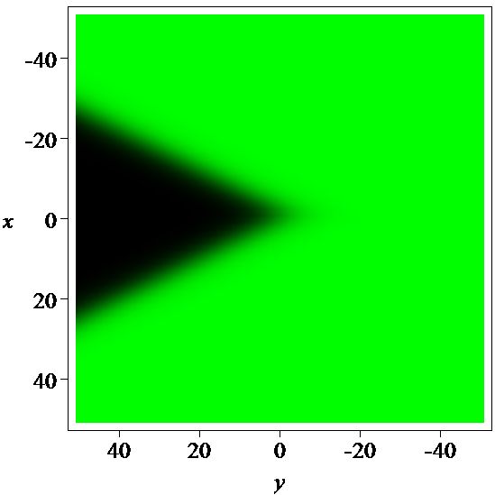
Figure 2. The profile of the solution of $q_{1}$(4.15) of equation (2.5) (left) and its density plot (right) with parameters $c=0,t_{3}=0,z=0.5,k=1$ and $n=1$.

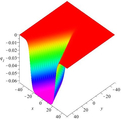
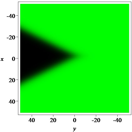
Figure 3. The profile of the solution of $q_{1}$(4.15) of equation (2.5) (left) and its density plot (right) with parameters $c=0,t_{3}=0,z=0.5,k=1$ and $n=2$.

 

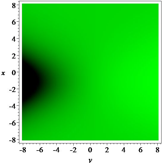
Figure 4. The profile of the solution $r_{1}$ (4.16) (left) of equation (2.5) and its density plot (right) with parameters $c=0,t_{3}=0,z=0.5,k=1$ and $n=0$. The vertical axis $r$ denotes the $r_{1}$.

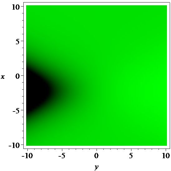
Figure 5. The profile of $r_{1}$ (4.16) (left) and its density plot (right) with parameters $c=0,t_{3}=0,z=0.5,k=1$ and $n=1$. The vertical axis $r$ denotes the $r_{1}$.

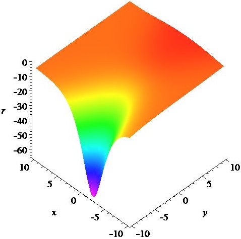
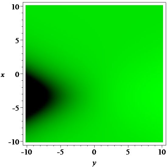
Figure 6. The profile of $r_{1}$ (4.16) (left) and its density plot (right) with parameters $c=0,t_{3}=0,z=0.5,k=1$ and $n=2$. The vertical axis $r$ denotes the $r_{1}$.

 

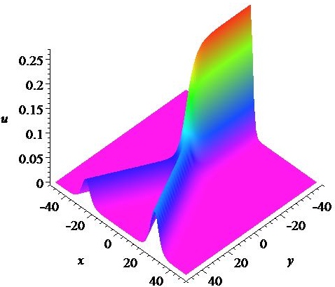
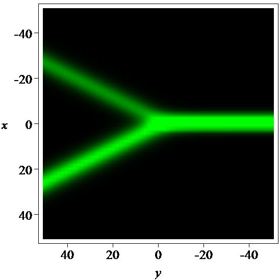
Figure 7. The profile of type Y soliton of $u_{1}$ (4.20) (left) and its density plot (right) with parameters $c=0,t_{3}=0,z=0.5,k=1$ and $n=0$. The vertical axis $u$ denotes the $u_{1}$.

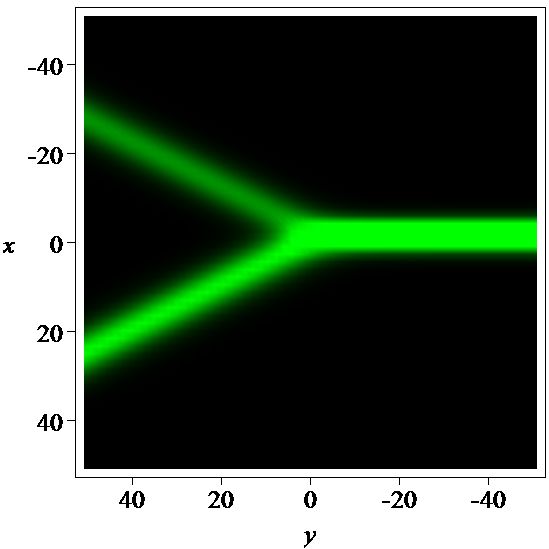
Figure 8. The profile of type Y soliton of $u_{1}$ (4.20) (left) and its density plot (right) with parameters $c=0,t_{3}=0,z=0.5,k=1$ and $n=1$. The vertical axis $u$ denotes the $u_{1}$.

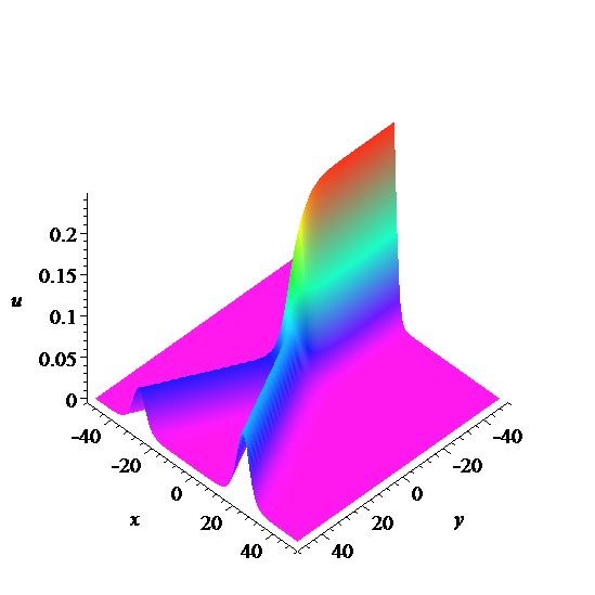
Figure 9. The profile of type Y soliton of $u_{1}$ (4.20) (left) and its density plot (right) with parameters $c=0,t_{3}=0,z=0.5,k=1$ and $n=2$. The vertical axis $u$ denotes the $u_{1}$.

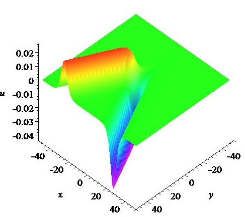
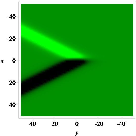
Figure 10. The profile of bright-dark type soliton of $u_{1}$ (4.21) (left) and its density plot (right) with parameters $c=0,t_{3}=0,z=0.5,k=2$ and $n=0$ . The vertical axis $u$ denotes the $u_{1}$.

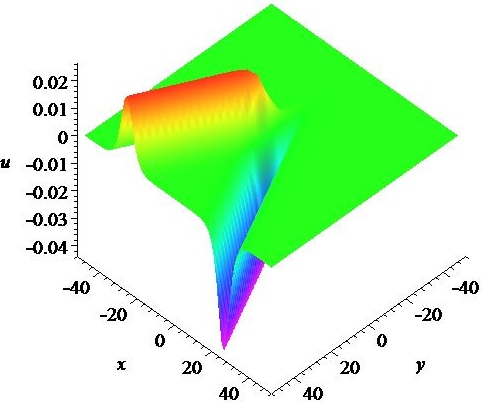
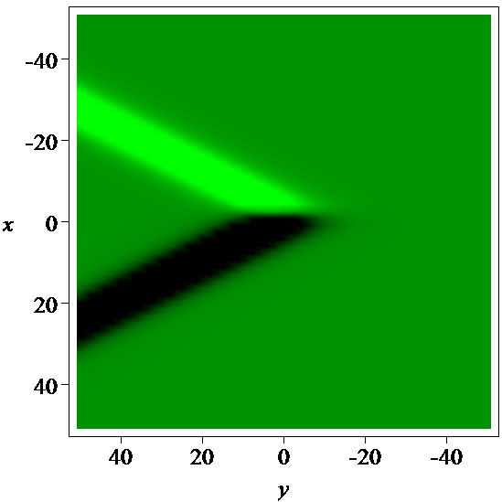
Figure 11. The profile of bright-dark type soliton of $u_{1}$ (4.21) (left) and its density plot (right) with parameters $c=0,t_{3}=0,z=0.5,k=2$ and $n=1$ . The vertical axis $u$ denotes the $u_{1}$.

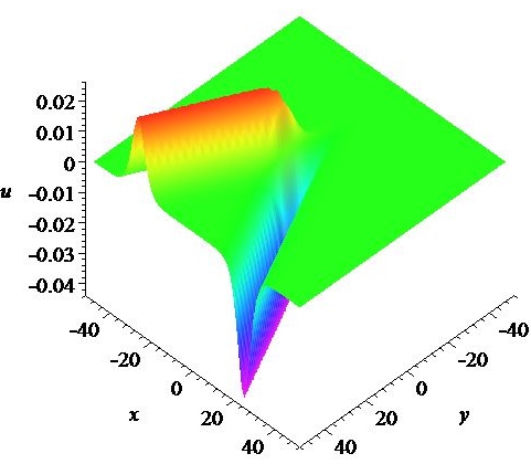
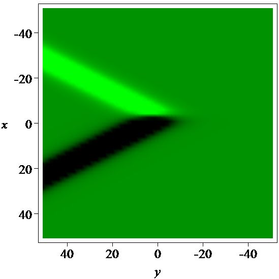
Figure 12. The profile of bright-dark soliton of $u_{1}$ (4.21) (left) and its density plot (right) with parameters $c=0,t_{3}=0,z=0.5,k=2$ and $n=2$. The vertical axis $u$ denotes the $u_{1}$.

(a)  (b)  (c)

Figure 13. $\Delta u_{1}(z,x,y,n)$ with $c=0,t_{3}=0,z=0.5,k=1$ and $n=1$ in (a), $2$ in (b) and $3$ in (c).