On a possibility to calculate fundamental parameters of the Standard Model

Abstract

The problem of a calculation of parameters of the Standard Model is considered in the framework of the compensation approach. Conditions for a spontaneous generation of effective interactions of fundamental fields are shown to lead to sets of equations for parameters of a theory. A principal possibility to calculate mass ratios of fundamental quarks and leptons is demonstrated, as well of mixing angles of quarks, e.g. of the Cabibbo angle. A possibility of a spontaneous generation of an effective interaction of electroweak gauge bosons $W^{a}$ and $B$ is demonstrated. In case of a realization of a non-trivial solution of a set of compensation equations, parameter $\sin^{2}\theta_{W}$ is defined. The non-trivial solution is demonstrated to provide a satisfactory value for the electromagnetic fine structure constant $\alpha$ at scale $M_{Z}$: $\alpha(M_{Z})=0.00772$. The results being obtained may be considered as sound arguments on behalf of a possibility of a calculation of parameters of the Standard Model.

PACS numbers: 11.15.Tk; 12.15.-y; 12.15.Ji; 12.90.+b; 14.70.Fm

1 Introduction

In works [1][7], N.N. Bogoliubov compensation principle [8, 9] was applied to studies of a spontaneous generation of effective non-local interactions in renormalizable gauge theories. The method and applications are also described in full in the book [10].

In particular, papers [4][6] deal with an application of the approach to the electro-weak interaction and a possibility of spontaneous generation of effective anomalous three-boson interaction of the form

$$-\,\frac{G}{3!}\,F\,\epsilon_{abc}\,W_{\mu\nu}^{a}\,W_{\nu\rho}^{b}\,W_{\rho\mu}^{c}\,;$$ (1)

$$W_{\mu\nu}^{a}\,=\,\partial_{\mu}W_{\nu}^{a}-\partial_{\nu}W_{\mu}^{a}\,+g\,\epsilon_{abc}W_{\mu}^{b}W_{\nu}^{c}\,.$$

with uniquely defined form-factor $F(p_{i})$, which guarantees effective interaction (1) acting in a limited region of the momentum space. It was done in the framework of an approximate scheme, which accuracy was estimated to be $\simeq(10-15)\%$ [1]. Would-be existence of effective interaction (1) leads to important non-perturbative effects in the electro-weak interaction. It is usually called anomalous three-boson interaction and it is considered for long time on phenomenological grounds [11, 12]. Our interaction constant $G$ is connected with conventional definitions in the following way

$$G\,=\,-\,\frac{g\,\lambda}{M_{W}^{2}}\,;$$ (2)

where $g\simeq 0.65$ is the electro-weak coupling. The best limitations for parameter $\lambda$ read [13]

$$\lambda_{\gamma}=-\,0.022\pm 0.019\,;\quad\lambda_{Z}=-\,0.09\pm 0.06\,;$$ (3)

where subscript denote a neutral boson being involved in the experimental definition of $\lambda$.

Solution of the analogous compensation procedure in QCD correspond to $g(z_{0})=3.8$ [7]. For the electro-weak interaction we have [5, 6]

$$g(z_{0})=0.60366\,;\quad z_{0}=9.6175\,;\quad|\lambda|=2.88\cdot 10^{-6}\,.$$ (4)

Here $z_{0}$ is a dimensionless parameter, which is connected with value of a boundary momentum, that is with effective cut-off $\Lambda$ according to the following definition [5, 6]

$$\frac{2\,G^{2}\,\Lambda^{4}}{1024\,\pi^{2}}\,=\,\frac{g^{2}\,\lambda^{2}\,\Lambda^{4}}{512\,\pi^{2}\,M_{W}^{4}}\,=\,z_{0}\,.$$ (5)

It is instructive to present in Fig. 1 the behavior of form-factor $F(p,-p,0)$ in dependence on momentum $p$, where

$$z\,=\,\frac{G^{2}\,p^{4}}{512\,\pi^{2}}\,;$$ (6)

and $F(z)\,=\,0$ for $z\,>\,z_{0}$.

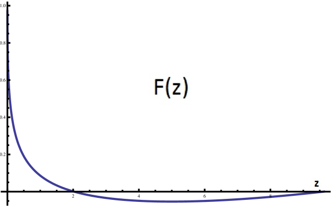
Figure 1: The behavior of the form-factor for the electro-weak theory.

As a rule the existence of a non-trivial solution of a compensation equation impose essential restrictions on parameters of a problem. Just the example of these restrictions is the definition of coupling constant $g(z_{0})$ in (4). It is advisable to consider other possibilities for spontaneous generation of effective interactions and to find out, which restrictions on physical parameters may be imposed by an existence of non-trivial solutions. In the present work we consider possibilities of definition of important physical parameters: mixing angles and mass ratios of elementary constituents of the Standard Model.

2 A model for mass relations of quarks and leptons

Following the approach used in works [1][7] let us formulate the compensation equations for would-be four-fermion interaction of two types of quarks and two leptons, that is we consider one generation of fundamental fermions. For the simplicity we call them $"u"$, $"d"$, $"e"$ and $"\nu"$, which in the standard way are represented by their left $\psi_{L}$ and right $\psi_{R}$ components. We admit initial masses for all participating fermions to be zero and we will look for possibility of them to acquire masses $m_{i},i=1,...4$ respectively due to interaction with scalar Higgs-like composite field.

Then let us consider a possibility of spontaneous generation of the following interaction, which is constructed by close analogy with the well-known Nambu – Jona-Lasinio effective interaction [14][18]

$$L_{eff}^{F}\,=\,G_{1}\bar{u}_{L}\,u_{R}\,\bar{u}_{R}\,u_{L}+G_{2}\bar{d}_{L}\,d_{R}\,\bar{d}_{R}\,d_{L}+G_{4}\bar{e}_{L}\,e_{R}\,\bar{e}_{R}\,e_{L}+$$

$$G_{3}(\bar{u}_{L}\,u_{R}\,\bar{d}_{R}\,d_{L}+\bar{d}_{L}\,d_{R}\,\bar{u}_{R}\,u_{L})+G_{5}(\bar{u}_{L}\,u_{R}\,\bar{e}_{R}\,e_{L}+\bar{e}_{L}\,e_{R}\,\bar{u}_{R}\,u_{L})+$$ (7)

$$G_{6}(\bar{e}_{L}\,e_{R}\,\bar{u}_{R}\,u_{L}+\bar{e}_{R}\,e_{L}\,\bar{u}_{L}\,u_{R})+G_{7}\,\bar{\nu}_{L}\,\nu_{R}\,\bar{\nu}_{R}\,\nu_{L}+$$

$$G_{8}(\bar{\nu}_{L}\,\nu_{R}\,\bar{d}_{R}\,d_{L}+\bar{d}_{L}\,d_{R}\,\bar{\nu}_{R}\,\nu_{L})+G_{9}(\bar{\nu}_{L}\,\nu_{R}\,\bar{u}_{R}\,u_{L}+\bar{u}_{L}\,u_{R}\,\bar{\nu}_{R}\,\nu_{L})+$$

$$G_{10}(\bar{\nu}_{L}\,\nu_{R}\,\bar{e}_{R}\,e_{L}+\bar{e}_{L}\,e_{R}\,\bar{\nu}_{R}\,\nu_{L}).$$

Here all coupling constants $G_{i}$ have dimension of the inverse mass squared $M^{-2}$.

Now we would like to find out, if the four-fermion interaction (10) could be spontaneously generated. In doing this we again proceed with the add-subtract procedure

$$L=L_{0}\,+\,L_{int}\,;\quad L_{int}\,=\,L_{0int}\,+\,L_{eff}^{F}\,;$$

$$L_{0}=\sum_{u,d}\bar{q}(x)(\imath\partial_{\alpha}\gamma_{\alpha}-m)q(x)+\sum_{e,\nu}\bar{l}(x)(\imath\partial_{\alpha}\gamma_{\alpha}-m)l(x)-L_{eff}^{F}\,;$$ (8)

here $L_{0int}$ is an initial interaction Lagrangian. Then we have to compensate the undesirable term $L_{eff}$ in the newly defined free Lagrangian. The relation, which serve to accomplish this goal, is called compensation equation. Necessarily we use approximate form of this equation. In diagram form the compensation equation for four fermions participating the interaction in one-loop approximation is presented in Fig. 2.

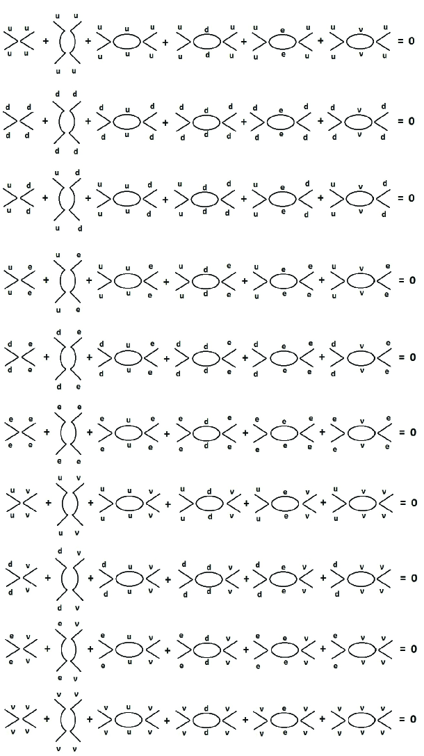
Figure 2: Diagram representation of the compensation equation for spontaneous generation of interaction (10). Notations of quarks and lepton are shown by corresponding lines.

Let us define effective cut-off $\Lambda$ in integrals of equation (10). We shall see below, that $\Lambda$ may be defined in the course of solution of compensation equations. With account of this definition we introduce the following dimensionless variables

$$y_{1}\,=\,\frac{G_{1}\,\Lambda^{2}}{8\,\pi^{2}}\,;\;y_{2}\,=\,\frac{G_{2}\,\Lambda^{2}}{8\,\pi^{2}}\,;\;y_{3}\,=\,\frac{G_{3}\,\Lambda^{2}}{8\,\pi^{2}}\,;$$

$$z_{1}\,=\,\frac{G_{4}\,\Lambda^{2}}{8\,\pi^{2}}\,;\;z_{2}\,=\,\frac{G_{7}\,\Lambda^{2}}{8\,\pi^{2}}\,;\;z_{3}\,=\,\frac{G_{10}\,\Lambda^{2}}{8\,\pi^{2}}\,;$$ (9)

$$x_{1}\,=\,\frac{G_{5}\,\Lambda^{2}}{8\,\pi^{2}}\,;\;x_{2}\,=\,\frac{G_{9}\,\Lambda^{2}}{8\,\pi^{2}}\,;\;x_{3}\,=\,\frac{G_{6}\,\Lambda^{2}}{8\,\pi^{2}}\,;$$

$$x_{4}\,=\,\frac{G_{8}\,\Lambda^{2}}{8\,\pi^{2}}\,;\;$$

$$\xi_{1}\,=\,\frac{m_{2}}{m_{1}}\,;\;\xi_{2}\,=\,\frac{m_{3}}{m_{1}}\,;\;\xi_{3}\,=\,\frac{m_{4}}{m_{1}}.$$

Then we consider scalar bound state consisting of all possible fermion-antifermion combinations $\bar{u}u$, $\bar{d}d$, $\bar{e}e$ and $\bar{\nu}\nu$. The corresponding set of Bethe-Salpeter equations is shown in Fig. 3. In this way we come to the following set of ten compensation equations presented in Fig. 2 and four Bethe-Salpeter equations shown in Fig. 3. Let us note, that in Fig. 3 we present also wouldbe contributions of gauge bosons exchanges, which in the calculations of the present section are not taken into account. Note also, that terms with factor $A$ arise from vertical diagrams in Fig. 2. Let us remind, that the sign minus before linear terms in compensation equations is connected with opposite signs of terms corresponding to effective interactions in the new free Lagrangian and in the new interaction Lagrangian.

$$-y_{1}\,+\,A\,y_{1}^{2}\,+\,3(y_{1}^{2}+y_{3}^{2})\,+\,x_{1}^{2}\,+\,x_{2}^{2}\,=0\,;$$

$$-y_{2}\,+\,A\,y_{2}^{2}\,\xi_{1}^{2}\,+\,3(y_{2}^{2}+y_{3}^{2})\,+\,x_{3}^{2}\,+x_{4}^{2}\,=0\,;$$

$$-y_{3}\,+\,A\,y_{3}^{2}\,\xi_{1}\,+\,3\,y_{3}(y_{1}+y_{2})\,+\,x_{1}\,x_{3}\,+\,x_{2}x_{4}\,=0\,;$$

$$-z_{1}\,+\,A\,z_{1}^{2}\,\xi_{2}^{2}\,+\,3\,(x_{1}^{2}+x_{3}^{2})\,+z_{1}^{2}\,+\,z_{3}^{2}\,=0\,;$$

$$-z_{2}\,+\,A\,z_{2}^{2}\,\xi_{3}^{2}\,+\,3\,(x_{2}^{2}+x_{4}^{2})\,+z_{2}^{2}\,+\,z_{3}^{2}\,=0\,;$$

$$-z_{3}\,+\,A\,z_{3}^{2}\,\xi_{2}\,\xi_{3}\,+\,3\,(x_{1}\,x_{2}+x_{3}\,x_{4})\,+\,z_{1}z_{3}\,+\,z_{2}z_{3}\,=0\,;$$

$$-x_{1}\,+\,A\,x_{1}^{2}\,\xi_{2}\,+\,3(x_{1}y_{1}+x_{3}y_{3})\,+\,x_{1}z_{1}\,+\,x_{2}z_{3}=\,0\,;$$ (10)

$$-x_{2}\,+\,A\,x_{2}^{2}\,\xi_{3}\,+\,3(x_{2}y_{1}+x_{3}y_{3})\,+\,x_{1}z_{1}\,+\,x_{2}z_{3}=\,0\,;$$

$$-x_{3}\,+\,A\,x_{3}^{2}\,\xi_{1}\,\xi_{2}+\,3(x_{1}y_{3}+x_{4}y_{3})\,+\,x_{1}z_{3}\,+\,x_{2}z_{2}\,=0\,;$$

$$-x_{4}\,+\,A\,x_{4}^{2}\,\xi_{1}\xi_{3}\,+\,3(x_{2}y_{3}+x_{4}y_{2})\,+\,x_{3}z_{3}\,+\,x_{4}z_{2}=\,0\,;$$

$$A\,=\,\frac{m_{u}^{2}}{4\,\Lambda^{2}}\,\ln\frac{\Lambda^{2}}{\bar{m}^{2}}\,;$$

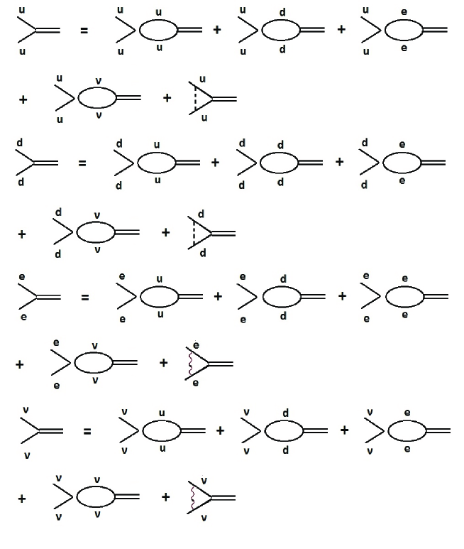
Figure 3: Diagram representation of the Bethe-Salpeter equation for scalar bound state, included in set of equations (11). Notations of quarks and lepton are shown by corresponding lines. Contributions of gauge bosons exchanges (the last diagrams in each equation) are not taken into account yet.

$$\frac{1}{B}\,=\,3(y_{1}\,+\,\xi_{1}\,y_{3})\,+\,\xi_{2}x_{1}\,+\,\xi_{3}x_{2};$$

$$\frac{\xi_{1}}{B}\,=\,3(y_{3}\,+\,\xi_{1}\,y_{2})\,+\,\xi_{2}\,x_{3}\,+\,\xi_{3}x_{4};$$ (11)

$$\frac{\xi_{2}}{B}\,=\,3(x_{1}\,+\,\xi_{1}\,x_{3})\,+\,\xi_{2}\,z_{1}\,+\,\xi_{3}z_{3};$$

$$\frac{\xi_{3}}{B}\,=\,3(x_{2}\,+\,\xi_{1}\,x_{4})\,+\,\xi_{2}\,z_{3}\,+\,\xi_{3}z_{2};$$

$$B\,=\,1\,+\,\frac{m_{0}^{2}}{2\,\Lambda^{2}}\,\ln\frac{\Lambda^{2}}{\bar{m}^{2}}\,;$$

where $m_{0}$ is the bound state mass and $\bar{m}$ is an average mass of participating fermions. Let us comment the appearance of mass parameters $\xi_{i}$ in terms, corresponding to vertical diagrams in Fig. 2. Due to the orthogonality of matrices

$$\frac{1+\gamma_{5}}{2}\,;\quad\frac{1-\gamma_{5}}{2}\,;$$ (12)

terms containing $\hat{q}$ cancel and we are left only with mass terms in spinor propagators. Introduction of the average $\bar{m}$, instead of substituting in proper places different masses $m_{i}$, means of course an approximation. However due to logarithmic dependence on this parameter, this approximation seems to be reasonable. Factor $A$ has to be very small and factor $B$ has to be close to unity, because $\Lambda\gg m_{i}$. Ten equations (10) correspond to the set of compensation equations, while four equations (11) represent the Bethe-Salpeter equations. Let us remind, that after performing the compensation procedure, which means exclusion of four-fermion vertices in the newly defined free Lagrangian, we use the resulting coupling constants in the newly defined interaction Lagrangian with the opposite sign.

The appearance of ratios $\xi_{i}$ in Bethe-Salpeter part (11) of the set presumably needs explanation. We assume, that the scalar composite state, which in our approach serves as a substitute of the elementary Higgs scalar, consists of all existing quark-antiquark and lepton-antilepton pairs $\bar{\psi}_{L}\,\psi_{R}$ (not only of heavy quarks $\bar{\Psi}_{L}\,\Psi_{R}$ as in work [5]). Then coupling of this scalar with different fermions will give their masses according to well known relation

$$g_{a}\,=\,\frac{g\,m_{a}}{\sqrt{2}\,M_{W}}\,.$$ (13)

On the other hand, Bethe-Salpeter wave functions are proportional to coupling constants $g_{a}$, where $a$ is just the constituent particle. Thus we change a ratio of coupling constants by a ratio of corresponding masses $\xi_{i}$.

In Section 3 we consider interaction of the Higgs field also with electroweak gauge bosons. Thus we assume, that the Higgs scalar consist of all existing fundamental massive fields. So in future studies it should be necessary to consider a set of Bethe-Salpeter equations including all possible constituents. Presumably it would be advisable to take into account also contributions of gauge interactions, which schematically presented in triangle diagrams of Fig. 3.

Now let us consider solutions of set (10, 11). First of all let us remind, that parameter $A$ is very small, so we look for solutions, which are stable in the limit $A\,\to\,0$. We also will consider only real solutions, because our variables just correspond to physical observable quantities. Namely, we have for $A\,=\,0.0001$ the following real solutions

$$y_{1}=0.12500,\;y_{2}=y_{1},\;y_{3}=-\,y_{1},$$

$$z_{1}=y_{1},\;z_{2}=y_{1},\;z_{3}=-\,y_{1},$$

$$x_{1}=y_{1},\;x_{2}=-\,y_{1},\;x_{3}=-\,y_{1},\;x_{4}=y_{1},$$ (14)

$$\xi_{1}=-\,1,\;\xi_{2}=1,\;\xi_{3}=-\,1,\;B=1.00001.$$

$$y_{1}=0.12500,\;y_{2}=y_{1},\;y_{3}=-\,y_{1},$$

$$z_{1}=y_{1},\;z_{2}=y_{1},\;z_{3}=y_{1},$$

$$x_{1}=y_{1},\;x_{2}=y_{1},\;x_{3}=-\,y_{1},\;x_{4}=-\,y_{1},$$ (15)

$$\xi_{1}=-\,1,\;\xi_{2}=1,\;\xi_{3}=1,\;B=1.00001.$$

$$y_{1}=0.24999,\;y_{2}=0.33333,\;y_{3}=0,$$

$$z_{1}=0.24999,\;z_{2}=0.56468,\;z_{3}=-\,0.38570,$$

$$x_{1}=-0.24999,\,x_{2}=x_{3}=x_{4}=0,$$ (16)

$$\xi_{1}=0.86603,\;\xi_{2}=-\,1,\;\xi_{3}=0,\;B=1.00003.$$

$$y_{1}=0.24999,\;y_{2}=0.33333,\;y_{3}=0,$$

$$z_{1}=0.24999,\;z_{2}=0.99998,\;z_{3}=0,$$

$$x_{1}=-0.24999,\,x_{2}=x_{3}=x_{4}=0,$$ (17)

$$\xi_{1}=0,\;\xi_{2}=1,\;\xi_{3}=0.5,\;B=1.000025.$$

$$y_{1}=0.33332,\;y_{2}=0,\;y_{3}=0,$$

$$z_{1}=0.24999,\;z_{2}=0.99998,\;z_{3}=0,$$

$$x_{1}=x_{2}=x_{3}=x_{4}=0,$$ (18)

$$\xi_{1}=0,\;\xi_{2}=\xi_{3}=0.57735,\;B=1.000033.$$

$$y_{1}=0.33332,\;y_{2}=0.057288,\;y_{3}=0,$$

$$z_{1}=0.26344,\;z_{2}=0.56470,\;z_{3}=-\,0.38570,$$

$$x_{1}=x_{2}=0,\;x_{3}=0.12285,\;x_{4}=-\,0.17986,$$ (19)

$$\xi_{1}=\xi_{2}=\xi_{3}=0,\;B=1.00003.$$

$$y_{1}=0.29077,\;y_{2}=0.29077,\;y_{3}=-\,0.04256,$$

$$z_{1}=0.25534,\;z_{2}=0,\;z_{3}=0,$$

$$x_{1}=0.17801,\,x_{2}=x_{4}=0,\,x_{3}=0.17801,$$ (20)

$$\xi_{1}=1,\;\xi_{2}=1.4344,\;\xi_{3}=0,\;B=1.00003.$$

$$y_{1}=0.19313,\;y_{2}=0.18758,\;y_{3}=0.14295,$$

$$z_{1}=0.857858,\;z_{2}=0,\;z_{3}=0,$$

$$x_{1}=-0.14116,\,x_{2}=x_{4}=0,\,x_{3}=0.14393,$$ (21)

$$\xi_{1}=1.069,\;\xi_{2}=0.26728,\;\xi_{3}=0,\;B=1.00002.$$

Of course, there is a temptation to confront these solutions with the existing generations of quarks and leptons. Let us note, that the first three solutions (14,15,16) contain mass ratios $\xi_{i}$ with negative signs, that is quite unnatural for fermions entering to one generation. In solutions (17, 18) there is no place for massless neutrino. However, these solutions may be tentatively considered in the framework of an option of wouldbe new generations with heavy neutrinos [19]. For the moment, the most suitable ones are the three last solutions (19, 20, 21). All these solutions have nonnegative parameters $\xi_{i}$ and at least one lepton being massless, that might be a neutrino. The solution (19) gives one (the first) fundamental fermion (quark) being much heavier, than three others, that reminds situation of the third generation with the very heavy $t$ quark. The solution (20) gives charged lepton mass approximately the same as those of quarks, that may hint the situation in the second generation with approximately equal masses of the muon and of the $s$-quark. The solution (21) gives two different masses for the quark pair, while the wouldbe charged lepton has the mass approximately four times smaller than that of the first quark. This resembles situation for the first generation. Indeed, let us take for the electron mass its physical value $m_{e}\,=\,0.51\,MeV$. Then we have from (21)

$$m_{e}\,=\,0.51\,MeV;$$

$$m_{u}\,=\,\frac{m_{e}}{\xi_{2}}\,=\,1.90\,MeV;$$ (22)

$$m_{d}\,=\,\frac{m_{e}\,\xi_{1}}{\xi_{2}}\,=\,2.04\,MeV.$$

The wouldbe $u$-quark mass fits into error bars of its definition, while the wouldbe $d$-quark mass is rather lighter than its physical value [13]. Note, that in our estimates we have not taken into account the phenomenon of mixing of down quarks ($d,\,s,\,b$).

Of course, the similarity is rather reluctant and there is no overall explicit agreement with the real situation. Maybe one could move further with an application of a next approximation, which presumably needs a consideration of the Bethe-Salpeter equations with account of gauge interactions contributions, that is with account of a gluon exchange and of electroweak bosons exchanges. These exchanges are schematically drawn in Fig. 3. The problem of an adequate formulation of the approximation needs a special investigation. Nevertheless, even a possibility to define ratios of the fundamental masses in the compensation approach is of a doubtless interest.

We would also draw attention to the important point, that for all solutions parameter $B$ is close to unity, just as we have expected . With decreasing of parameter $A$, which is proportional to ratio squared of the mass of the first quark and cut-off $\Lambda$, parameter $B$ tends to unity exactly. Emphasize, that solutions  (20, 21) are stable in respect to $A\to 0$.

Let us estimate also order of magnitude of mixing angles between generations. For the purpose we introduce in effective interaction (7) additional terms, corresponding to the wouldbe $s,\,d$ mixing.

$$\Delta\,L\,=\,\frac{8\pi^{2}}{\Lambda^{2}}\Bigr{(}y_{12}\bigl{(}(\bar{s}^{\prime}_{R}\,d^{\prime}_{L}+\bar{d}^{\prime}_{R}\,s^{\prime}_{L})\bar{d}^{\prime}_{L}d^{\prime}_{R}+(\bar{s}^{\prime}_{L}\,d^{\prime}_{R}+\bar{d}^{\prime}_{L}\,s^{\prime}_{R})\bar{d}^{\prime}_{R}d^{\prime}_{L}\bigl{)}+$$

$$y_{32}\bigr{(}(\bar{s}^{\prime}_{R}\,d^{\prime}_{L}+\bar{d}^{\prime}_{R}\,s^{\prime}_{L})\bar{s}^{\prime}_{L}s^{\prime}_{R}+(\bar{s}^{\prime}_{L}\,d^{\prime}_{R}+\bar{d}^{\prime}_{L}\,s^{\prime}_{R})\bar{s}^{\prime}_{R}s^{\prime}_{L}\bigl{)}+$$ (23)

$$y_{52}(\bar{s}^{\prime}_{L}d^{\prime}_{R}\bar{d}^{\prime}_{R}s^{\prime}_{L}+\bar{s}^{\prime}_{R}d^{\prime}_{L}\bar{d}^{\prime}_{L}s^{\prime}_{R})+t_{32}(\bar{d}^{\prime}_{L}d^{\prime}_{R}\bar{s}^{\prime}_{L}s^{\prime}_{R}+\bar{d}^{\prime}_{R}d^{\prime}_{L}\bar{s}^{\prime}_{R}s^{\prime}_{L})\Bigr{)};$$

We have also mixing in mass terms of the two spinor fields $d^{\prime},\,s^{\prime}$

$$-m_{u}\bigl{(}\bar{u}u\,+\,\xi_{1}\bar{d}^{\prime}d^{\prime}\,+\,\xi_{4}\bar{s}^{\prime}s^{\prime}\,+\,\xi_{6}(\bar{s}^{\prime}d^{\prime}\,+\,\bar{d}^{\prime}s^{\prime})\bigr{)}\,;$$ (24)

where, as well as in expression (23), $d^{\prime},\,s^{\prime}$ are mixed states of physical $d$ and $s$

$$d^{\prime}\,=\,\cos\phi\,d\,+\,\sin\phi\,s\,;\;s^{\prime}\,=\,-\,\sin\phi\,d\,+\,\cos\phi\,s\,;$$ (25)

and $\phi$ is the well known Cabibbo angle.

Now we have in addition to parameters in (23) parameter $y_{2}$ from (9), which corresponds to term $\bar{d}d\bar{d}d$ and we also introduce the analogous parameter $y_{21}$, corresponding to term $\bar{s}s\bar{s}s$. These variables will be fixed by results (19 - 21). We now neglect all other transitions but those between $d$ and $s$ states and thus we have the following set of equations

$$-y_{12}+Ay_{12}+3(y_{12}y_{2}+y_{32}t_{32}+2\,y_{52}y_{12})=0\,;$$

$$-y_{32}+Ay_{32}+3(y_{12}t_{32}+y_{32}y_{21}+2\,y_{52}y_{32})=0\,;$$

$$-y_{52}+Ay_{52}+3(y_{12}^{2}+y_{32}^{2}+2\,y_{52}^{2})\,;$$

$$-t_{32}+At_{32}+3(y_{2}t_{32}+y_{21}t_{32}+y_{12}y_{32})\,$$ (26)

$$\frac{\xi_{1}}{B}=3(y_{2}\xi_{1}+t_{32}\xi_{4}+2\,y_{12}\xi_{6})\,;$$

$$\frac{\xi_{4}}{B}=3(t_{32}\xi_{1}+y_{21}\xi_{4}+2\,y_{32}\xi_{6})\,;$$

$$\frac{\xi_{6}}{B}=3(y_{12}\xi_{1}+y_{32}\xi_{4}+2\,y_{52}\xi_{6})\,.$$

The set has many solutions, mostly the complex ones. We consider only real solutions and choose such ones, which allow physical interpretation. Thus we shall consider several examples and postpone for future studies the problem of an explanation, why just the solutions being considered correspond to real physics. Maybe this problem is connected with properties of a stability of solutions.

Fixing values for $y_{2}$ and $y_{21}$ from results (20, 21) and value $A$ we obtain seven equations for seven variables: $y_{12},\,y_{32},\,y_{52},\,t_{32},\,B,\,\xi_{1}/\xi_{6},\,\xi_{4}/\xi_{6}$. Let us check if there will be a reasonable mixing of solutions (20, 21) that is between the first two generations according to our guess. With $y_{2}=0.18758,\,y_{21}=0.29077,\,A=0.000005,\,\xi_{6}=1$ we have the following solution

$$y_{12}=-0.0000003158,\;y_{32}=0.078656,\;y_{52}=0.0212768,$$

$$t_{32}=-0.000000943,\;\xi_{1}=-0.0000282,\;\xi_{4}=3.69675,\;B=1.00003\,.$$ (27)

As well as solutions (20, 21), this solution is also stable in respect to $A\to 0$. It is easy to see, that parameters $\xi_{1,4}$ give values of a mixing angle $s$ and a ratio of masses R according to the following set of equations

$$s\,=\,\sin\phi\,;\quad R\,=\,\frac{m_{s}}{m_{d}}\,;$$ (28)

$$(\xi_{1}-\xi_{4})s\sqrt{1-s^{2}}+\xi_{6}(1-2s^{2})=0\,,\quad R=\frac{y+\sqrt{x^{2}+1}}{\sqrt{x^{2}+1}-y};$$

$$x=\frac{\xi_{4}-\xi_{1}}{2},\;y=\frac{\xi_{1}+\xi_{4}}{2}\,.$$

For data (27) we have the following two solutions

$$s_{1}\,=\,0.2454,\quad R_{1}\,=\,15.6;$$ (29)

$$s_{2}\,=\,-\,0.9694,\quad R_{2}\,=\,15.6.$$ (30)

Let us note, that $s_{1}^{2}+s_{2}^{2}=1$ and $R_{1}\,=\,R_{2}$ exactly.

Solution (29) may be compared with real situation of $(d,\,s)$ mixing, because mass ratio $R\,=\,m_{s}/m_{d}$ is close to its actual value and the mixing angle is also not far from actual Cabibbo angle value [13]

$$\sin\phi_{c}\,=\,s\,=\,0.2254\pm 0.0006\,;\quad\frac{m_{s}}{m_{d}}\,=\,R\,=\,19.8^{+2.4}_{-2.8}\,.$$ (31)

Let us try to proceed to the next approximation, that means inclusion to the analysis of up quarks also. This means consideration of the following effective interaction to be added to expressions (7, 23)

$$\Delta^{\prime}L=\frac{8\pi^{2}}{\Lambda^{2}}\Bigl{(}t_{21}(\bar{u}_{L}u_{R}\bar{s}^{\prime}_{R}s^{\prime}_{L}+\bar{u}_{R}u_{L}\bar{s}^{\prime}_{L}s^{\prime}_{R})+t_{22}(\bar{u}_{L}u_{R}\bar{c}_{R}c_{L}+\bar{u}_{R}u_{L}\bar{c}_{L}c_{R})+$$

$$y_{22}\bigl{(}\bar{u}_{L}u_{R}(\bar{s}^{\prime}_{R}d^{\prime}_{L}+\bar{d}^{\prime}_{R}s^{\prime}_{L})+\bar{u}_{R}u_{L}(\bar{s}^{\prime}_{L}d^{\prime}_{R}+\bar{s}^{\prime}_{R}d^{\prime}_{L})+h.c.\bigr{)}+y_{11}\bar{c}_{L}c_{R}\bar{c}_{R}c_{L}+$$

$$y_{21}\bar{s}^{\prime}_{L}s^{\prime}_{R}\bar{s}^{\prime}_{R}s^{\prime}_{L}+y_{42}\bigl{(}\bar{c}_{L}c_{R}(\bar{s}^{\prime}_{R}d^{\prime}_{L}+\bar{d}^{\prime}_{R}s^{\prime}_{L})+\bar{c}_{R}c_{L}(\bar{s}^{\prime}_{L}d^{\prime}_{R}+\bar{s}^{\prime}_{R}d^{\prime}_{L})+h.c.\bigr{)}+$$

$$t_{31}(\bar{s}^{\prime}_{L}s^{\prime}_{R}\bar{c}_{R}c_{L}+\bar{s}^{\prime}_{R}s^{\prime}_{L}\bar{c}_{L}c_{R})\Bigr{)}\,.$$ (32)

Bearing in mind the stability property of solutions (20, 21, 27) in respect to $A\to 0$, we put $A=0$ (that simplifies the hunting for solutions), and using for additional interaction (32) the same rules as previously, we obtain the following set of equations

$$-y_{1}+3(y_{1}^{2}+y_{3}^{2}+t_{21}^{2}+t_{22}^{2}+y_{22}^{2})=0;\;-y_{2}+3(y_{2}^{2}+y_{3}^{2}+t_{31}^{2}+t_{32}^{2}+y_{12}^{2})=0;$$

$$-y_{3}+3(y_{3}(y_{1}+y_{2})+t_{21}t_{31}+t_{22}t_{32}+y_{22}y_{12});$$

$$-y_{12}+3(y_{12}y_{2}+y_{22}y_{3}+y_{32}t_{32}+y_{42}t_{31}+2\,y_{52}y_{12})=0;$$

$$-y_{22}+3(y_{22}y_{1}+y_{12}y_{3}+y_{32}t_{22}+y_{42}t_{31}+2\,y_{52}y_{22})=0;$$

$$-y_{32}+3(y_{12}t_{32}+y_{22}t_{22}+y_{32}y_{21}+y_{42}y_{31}+2\,y_{52}y_{32})=0;$$

$$-y_{42}+3(y_{12}t_{31}+y_{22}t_{21}+y_{32}y_{31}+y_{42}y_{11}+2\,y_{52}y_{42})=0;$$

$$-y_{52}+3(y_{12}^{2}+y_{22}^{2}+y_{32}^{2}+y_{42}^{2}+2\,y_{52}^{2})=0;$$ (33)

$$-t_{21}+3(y_{1}t_{21}+y_{3}t_{31}+t_{21}y_{11}+t_{22}y_{31}+y_{22}y_{42})=0;$$

$$-t_{22}+3(y_{1}t_{22}+y_{3}t_{32}+t_{21}y_{31}+t_{22}y_{21}+y_{22}y_{32})=0;$$

$$-t_{31}+3(y_{3}t_{21}+y_{2}t_{31}+t_{31}y_{11}+t_{32}y_{31}+y_{12}y_{42})=0;$$

$$-t_{32}+3(y_{3}t_{22}+y_{2}t_{32}+t_{31}y_{31}+t_{32}y_{21}+y_{12}y_{32})=0;$$

$$3(t_{21}^{2}+t_{31}^{2}+2y_{42}^{2}+y_{31}^{2}+y_{11}^{2})=y_{11};\;3(y_{21}^{2}+y_{31}^{2}+2y_{32}^{2}+t_{22}^{2}+t_{32}^{2})=y_{21};$$

$$-y_{31}+3(y_{11}y_{31}+y_{21}y_{31}+2y_{32}y_{42}+t_{21}t_{22}+t_{31}t_{32})=0;$$

$$1=3B(y_{1}+y_{3}\xi_{1}+2y_{22}\xi_{6}+t_{21}\xi_{3}+t_{22}\xi_{4});$$

$$\xi_{1}=3B(y_{3}+y2\xi_{1}+2y_{12}\xi_{6}+t_{31}\xi_{3}+t_{32}\xi_{4});$$

$$\xi_{3}=3B(t_{21}+t_{31}\xi_{1}+y_{11}\xi_{3}+y_{31}\xi_{4}+2y_{42}\xi_{6});$$

$$\xi_{4}=3B(t_{22}+t_{32}\xi_{1}+y_{31}\xi_{3}+y_{21}\xi_{4}+2y_{32}\xi_{6});$$

$$\xi_{6}=3B(y_{22}+y_{12}\xi_{1}+y_{42}\xi_{3}+y_{32}\xi_{4}+2\,y_{52}\xi_{6}).$$

Here $B$, which has to be equal to unity, is the same as in (26). Additional mass parameters are defined in the following way by extending  (24) to the following expression

$$-m_{u}\bigl{(}\bar{u}u\,+\,\xi_{1}\bar{d}^{\prime}d^{\prime}\,+\,\xi_{3}\bar{c}c\,+\,\xi_{4}\bar{s}^{\prime}s^{\prime}\,+\,\xi_{6}(\bar{s}^{\prime}d^{\prime}\,+\,\bar{d}^{\prime}s^{\prime})\bigr{)}\,;$$ (34)

There is a solution of set (33), which is close to previous one (29). Namely it looks like for A=0

$$y_{1}=0.1773,\;y_{2}=0.1571,\;y_{3}=0.16583,\;y_{11}=0.3329,\;y_{21}=0.3327,$$

$$y_{31}=0.00052098,\;y_{12}=y_{22}=y_{32}=y_{42}=0,\;y_{52}=0.166667,$$ (35)

$$t_{21}=0.0082035,\;t_{22}=-0.0099095,\;t_{31}=-0.0087183,\;t_{32}=0.010531,\;$$

$$\xi_{1}=1.190304,\;\xi_{3}=9.97278,\;\xi_{4}=12.42852,\,\xi_{6}=2.68897.$$

Solution (35) gives the following results for parameters (28)

$$s\,=\,0.221,\quad R\,=\,22.43.$$ (36)

We see, that this result agrees actual values (31) even better than result (29). That is we may state the improvement of results in the course of successive approximations.

As a matter of fact solution (35) gives the wouldbe $c$-quark mass only ten times more than that of the $u$-quark. However, one may expect strong influence on this relation of a mixing with the heavy $t$-quark. Thus the approximation, which we demonstrate here is applied just for consideration of the $d\,s$ mixing.

The examples being just considered shows possibility of definition of mass ratios and of some mixing angles in the compensation approach. There are also other mixing angles in the Standard Model, first of all, the famous Weinberg angle $\theta_{W}$ in $W^{0},\,B$ mixing. In the next section we consider a possible way of calculation of this important parameter following the same approach.

3 Weinberg mixing angle and the fine structure constant

Let us demonstrate a simple model, which illustrates how the well-known Weinberg mixing angle could be defined. Let us consider a possibility of a spontaneous generation of the following effective interaction of electroweak gauge bosons

$$L_{eff}^{W}=G_{1}W^{a}_{\mu}W^{d}_{\mu}\,W^{a}_{\rho\sigma}W^{d}_{\rho\sigma}+G_{2}W^{a}_{\mu}W^{a}_{\mu}W^{b}_{\rho\sigma}W^{b}_{\rho\sigma}+$$

$$G_{3}\,W^{a}_{\mu}W^{a}_{\mu}B_{\rho\sigma}B_{\rho\sigma}+G_{4}\,Z_{\mu}Z_{\mu}W^{b}_{\rho\sigma}W^{b}_{\rho\sigma}+G_{5}\,Z_{\mu}Z_{\mu}B_{\rho\sigma}B_{\rho\sigma}.$$ (37)

where we maintain the residual gauge invariance for the electromagnetic field. Here indices $a,d$ correspond to charged $W$-s, that is they take values $1,\,2$, while index $b$ corresponds to three components of $W$ defined by the initial formulation of the electro-weak interaction. Let us remind the relation, which connect fields $W^{0},\,B$ with physical fields of the $Z$ boson and of the photon

$$W^{0}_{\mu}=\cos\theta_{W}\,Z_{\mu}+\sin\theta_{W}\,A_{\mu};$$

$$B_{\mu}=-\,\sin\theta_{W}\,Z_{\mu}+\cos\theta_{W}\,A_{\mu}.$$ (38)

Interactions of type (37) were earlier introduced on phenomenological grounds in works [20, 21]. Let us introduce an effective cut-off $\Lambda$ in the same way as we have done in the previous section and use for definition of $\Lambda$ relation (5). Here we shall proceed just in the same way as earlier. Then let us consider a possibility of a spontaneous generation of interaction (37). In doing this we again proceed with the add-subtract procedure, which was used throughout works [1][6]. Now we start with usual form of the Lagrangian, which describes electro-weak gauge fields $W^{a}$ and $B$

$$L=L_{0}\,+\,L_{int}\,;$$

$$L_{0}=-\,\frac{1}{4}\bigl{(}W_{0\mu\nu}^{a}\,W_{0\mu\nu}^{a}\bigr{)}\,-\,\frac{1}{4}\bigl{(}B_{\mu\nu}\,B_{\mu\nu}\bigr{)}\,;$$ (39)

$$L_{int}\,=\,-\frac{1}{4}\bigl{(}W_{\mu\nu}^{a}\,W_{\mu\nu}^{a}-W_{0\mu\nu}^{a}\,W_{0\mu\nu}^{a}\bigr{)}\,.$$ (40)

$$W_{0\mu\nu}^{a}=\partial_{\mu}W_{\nu}^{a}-\partial_{\nu}W_{\mu}^{a};\;B_{\mu\nu}=\partial_{\mu}B_{\nu}-\partial_{\nu}B_{\mu}.$$

and $W_{\mu\nu}^{a}$ is the well-known non-linear Yang-Mills field of $W$-bosons. Then we perform the add-subtract procedure of expression (37)

$$L=L^{\prime}_{0}\,+\,L^{\prime}_{int}\,;$$

$$L^{\prime}_{0}=L_{0}\,-\,L_{eff}^{W}\,;$$ (41)

$$L^{\prime}_{int}\,=\,L_{int}\,+\,L_{eff}^{W}\,.$$ (42)

Now let us formulate compensation equations. We are to demand, that considering the theory with Lagrangian $L^{\prime}_{0}$ (41), all contributions to four-boson connected vertices, corresponding to interaction (37) are summed up to zero. That is the undesirable interaction part in the would-be free Lagrangian (41) is compensated. Then we are rested with interaction (37) only in the proper place (42) We have the following set of compensation equations, which corresponds to diagrams being presented in the first six rows of Fig. 4

$$-\,x_{1}\,+\,x_{1}^{2}\,=\,0\,;$$

$$-\,x_{2}\,+\,2\,x_{2}^{2}\,+\,2\,x_{1}x_{2}\,+\,(1-a^{2})\,x_{3}x_{4}\,+$$

$$a^{2}\,x_{2}x_{4}=\,0\,;$$

$$-\,x_{3}\,+\,x_{1}x_{3}\,+\,2\,x_{2}x_{3}\,+\,a^{2}\,x_{2}\,x_{5}\,+$$

$$(1-a^{2})\,x_{3}x_{5}\,=\,0\,;$$ (43)

$$-\,x_{4}\,+\,x_{1}x_{4}\,+\,2\,x_{2}x_{4}\,+\,a^{2}\,x_{4}x_{5}\,=\,0\,;$$

$$-\,x_{5}\,+\,2\,x_{3}x_{4}\,+\,a^{2}\,x_{4}\,x_{5}\,+\,(1-a^{2})\,x_{5}^{2}\,=\,0\,;$$

$$x_{i}\,=\,\frac{3\,G_{i}\,\Lambda^{2}}{64\,\pi^{2}}\,;\quad a\,=\,\cos\theta_{W}\,.$$

Factor $2$ in several terms of equations here corresponds to sum by weak isotopic index $\delta^{a}_{a}\,=\,2,\,a=1,\,2$.

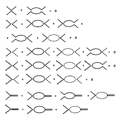
Figure 4: Diagram representation of set (43) (the first five equations) and (44) (the two last ones). Simple line represent $W$-s, dotted lines represent $B$ and lines, consisting of black spots, represent $Z$. Double lines represent the Higgs scalar.

Then, following the reasoning of the approach, we assume, that the Higgs scalar corresponds to a bound state consisting of a complete set of fundamental particles. Note, that in work [5] we have considered only the heaviest particle $t$ quark as the main constituent of the Higgs scalar. Here we are to include the electro-weak bosons. There are two Bethe-Salpeter equations for this bound state, because constituents are either $W^{a}\,W^{a}$ or $Z\,Z$. These equations are presented in the last two rows of Fig. 4. In approximation of very large cut-off $\Lambda$ these equations have the following form

$$x_{1}\,+(2\,+\,a)\,x_{2}\,+\,\frac{1-a^{2}}{a}\,x_{3}\,+\,\beta\,=\,1\,;$$ (44)

$$(2\,+\,a)\,x_{4}\,+\,\frac{1-a^{2}}{a}\,x_{5}\,+\,\frac{\beta}{a}\,=\,\frac{1}{a}\,.$$

Here we introduce parameter $\beta$, which describes wouldbe additional contributions. We consider as physical solutions those with very small $\beta$. Now we look for solutions of set (43, 44) for variables $x_{i},\,a,\,\beta$. Of course, there is the trivial solution: all $x_{i}\,=\,0,\,\beta\,=\,1$. However there are also non-trivial solutions. Namely, there are the the following two ones with $x_{1}\,=\,1$

$$x_{2}\,=\,0\,;\;x_{3}\,=\,0.729625\,;\;x_{4}\,=\,0\,;\;x_{5}\,=\,0\,;$$ (45)

$$\beta_{1}\,=\,1\,;\;\beta_{2}\,=\,\frac{0.729625\,(a-1)}{a}\,;$$

for any $a$, and the following three ones with $x_{1}\,=\,0$

$$x_{2}\,=\,0\,,\;x_{3}\,=\,3.070337\,,\;x_{4}\,=\,0\,,\;x_{5}\,=\,3.61378\,,$$

$$a\,=\;0.8504594\,,\;\beta\,=\,-\,5.06\cdot 10^{-16}\,;$$ (46)

$$x_{2}\,=\,0.48772\,,\;x_{3}\,=\,0\,,\;x_{4}\,=\,1.2654\,,\;x_{5}\,=\,0\,,$$

$$a\,=\,0.33801\,,\;\beta\,=\,-\,1.2\cdot 10^{-5}\,;$$

$$x_{2}\,=\,0.5\,,\;x_{3}\,=\,1.09555\,,\;x_{4}\,=\,0\,,\;x_{5}\,=\,0\,,$$

$$a\,=\,-\,0.75556\,,\;\beta=\,1\,.$$

Very small $\beta$ are appropriate for the first solution of (46) with $\beta\simeq-\,5\cdot 10^{-16}$ and for the second one with $\beta\simeq-\,1.2\cdot 10^{-5}$. Note, that for solutions (45) smallness of $\beta$ is achieved only for the second one with $a\,\to\,1$, that is in an absence of the mixing. The solution with the smallest $\beta$ gives for the mixing parameter

$$\sin^{2}\theta_{W}\,=\,1-a^{2}\,=\,0.27672\,.$$ (47)

This value corresponds to scale $\Lambda$ (5), which is defined by parameter $z_{0}$. At this scale the electroweak coupling according to (4) is the following

$$\alpha_{ew}(z_{0})\,=\,\frac{g(z_{0})^{2}}{4\,\pi}\,=\,0.028999\,.$$ (48)

Then we obtain the electromagnetic coupling at the same scale

$$\alpha(z_{0})\,=\,\alpha_{ew}(z_{0})\,\sin^{2}\theta_{W}(z_{0})\,=\,0.0080244\,.$$ (49)

With the well-known evolution expression for electromagnetic coupling we have for six quark flavors ($\Lambda\gg M_{W}$)

$$\alpha(z_{0})\,=\,\frac{\alpha(M_{Z})}{1-\frac{5\alpha(M_{Z})}{6\,\pi}\ln\bigl{[}\frac{\Lambda^{2}}{M_{Z}^{2}}]}\,=\,0.0080244\,.$$ (50)

This gives for value $\Lambda$ from expression (5) with an account of (4)

$$\alpha(M_{Z})\,=\,0.007719\,.$$ (51)

to be compared with experimental value [13]

$$\alpha(M_{Z})\,=\,0.0077562\pm 0.0000012.$$ (52)

Of course, set of equations (43, 44) is approximate. It quite may be, that with an account of necessary corrections the agreement of the result with experimental number (52) will be not such indecently good. For example, provided we take the value of boundary momentum $\Lambda$ being an order of magnitude up and down of that defined by relations (4), we have

$$\alpha(M_{Z})_{up}\,=\,0.00765\,;\quad\alpha(M_{Z})_{down}\,=\,0.00779\,.$$ (53)

The second solution gives mach larger value for $\sin^{2}\theta_{W}\simeq 0.89$. As a result this leads to $\alpha(M_{Z})\simeq 0.0235$, that is three times more, than (51, 52). Now we have one solution (51) being in agreement with actual physics and another one being in evident disagreement. Which one is to be used?

The answer is connected with the problem of a stability of solutions (46). The stability in the model is defined by sum of vacuum averages

$$\frac{1}{4}<W_{\mu\nu}^{a}\,W_{\mu\nu}^{a}>\,+\,\frac{1}{4}<B_{\mu\nu}\,B_{\mu\nu}>\,.$$ (54)

A calculation of these vacuum averages even in the first approximation needs knowledge of explicit form-factors in effective interactions (37). To achieve this knowledge one has to perform the next step in a formulation and a solution of compensation equations, namely, it is necessary to take into account two-loop terms in compensation equations in analogy to works [2, 3]. This procedure is to be considered elsewhere. For the moment we may only state, that one of two possible solutions gives satisfactory value for fine structure constant $\alpha(M_{W})$. On the other hand, let us note the following. Provided the form-factor will be qualitatively the same as is presented in Fig. 1, i.e. being negative for large momenta, preliminary estimates show, that just the solution with value $\alpha(M_{W})$ (51) is more stable than other one. Maybe it is worth mentioning, that the preferable solution contains only combination $B_{\mu\nu}B_{\mu\nu}$ in effective interaction (37), while the solution with large $\alpha(M_{W})$ on the contrary contains only combination $W^{b}_{\mu\nu}W^{b}_{\mu\nu}$.

The results being demonstrated can not be regarded as finally decisive ones and are rather indications of how things might occur. However in view of a fundamental importance of a possibility to define parameters of the Standard Model, we do present these considerations. Additional arguments on behalf of our point of view are presented in the subsequent section.

4 Conclusion

Possible way of determination of fundamental fermion mass ratios, of mixing angles in the Cabibbo-Kobayashi-Maskawa matrix and of the Weinberg mixing angle, which is proposed in the work needs further studies, especially in respect to the next approximations. As well problems of stability, which might choose appropriate solutions, need thorough consideration. Thus we can not consider results being described here as final ones. They are just examples, which illustrate how things may occur.

In any case the examples being considered in the present work show, that a consideration of effective interactions in the compensation approach might lead to a determination of fundamental parameters of the Standard Model including the Weinberg mixing angle, mass ratios of fundamental particles and the Cabibbo angle. Remind, that a result being obtained above give quite a satisfactory value for the most important physical parameter – the fine structure constant $\alpha$. We would also draw attention to an appearance of very small numbers in solutions being considered. E.g. solution (46) contains parameter $\beta\simeq 5\cdot 10^{-16}$. This might be useful in application to problems of hierarchy [22, 23].

Let us emphasize, that the possibility of an adequate definition of the fundamental parameters of the Standard Model, is alternative to the option of anthropic principle (see recent works and reviews [24][27] and papers quoted therein), which assumes multiplicity of Universes. The main foundation of this postulate is just an absence of any mechanism, which could fix values of parameters of the Standard Model. The number $N_{SM}$ of fundamental parameters of the Standard Model including those, which are related to neutrinos, may be estimated to be as large as 25. Because each possible set of these parameters corresponds to a really existing Universe, the power of the set of the totality of Universes corresponds to the continuum. On the other hand, the existence of a human being, who is capable to observe the Nature and to try to understand Its laws, is closely connected with actual values of the parameters of the Standard Model. The properties of nuclei are connected with parameters defining low-energy strong interaction, that is the average strong coupling at low energies $\bar{\alpha}_{s}$ and light quark masses $m_{u},\,m_{d}$. The most important parameters, which define the rich variety of organic substances, which is inevitably necessary for the life generation and evolution, are just the fine structure constant $\alpha$ and the electron mass $m_{e}$. We have discussed in the present work possibilities for determination of all these fundamental parameters, but strong coupling $\bar{\alpha}_{s}$, which was considered in work [7].

Thus the anthropic principle assumes, that we live in the only Universe, which supplies conditions for an existence of a human being, that is in the Universe with such parameters $\alpha,\,\bar{\alpha}_{s},\,m_{u},\,m_{d},\,m_{e}$, which we consider now as real physical ones. All other Universes are deprived of an observer and so are principally unobservable.

The approach, which we have used in the present work, provides a possibility to define at least some of these parameters. Indeed, in work [7] we have obtained value of average strong coupling in the low-momenta region $\bar{\alpha}_{s}\simeq 0.85$ in agreement with its phenomenological value. As for other parameters, in the present work we just discuss examples of definition of the fine structure constant and light mass ratios in the framework of a spontaneous generation of effective interactions in the Standard Model. Relations (4, 22, 29, 36, 51) seemingly can not be yet considered being decisive ones, but the examples, which give these results, may serve as leading indications for further more detailed studies. In case of a realization of the program, we would obtain an understanding of how values of the fundamental parameters are fixed. Then the conception of the uniqueness of the Universe might be established. That is, it might be, that the observable Universe corresponds to the most stable non-trivial solution of the Standard Model. The authors do express the conviction, that a possible way to this goal is connected with a phenomenon of a spontaneous generation of effective interactions in the framework of the Standard Model.

5 Acknowledgments

The work is supported in part by the Russian Ministry of Education and Science under grant NSh-3042.2014.2.

References

[1] B. A. Arbuzov, Theor. Math. Phys., 140, 1205 (2004);
[2]B. A. Arbuzov, Phys. Atom. Nucl., 69, 1588 (2006).
[3]B. A. Arbuzov, M. K. Volkov and I. V. Zaitsev, Int. J. Mod.
Phys. A, 21, 5721 (2006).
[4]B. A. Arbuzov, Eur. Phys. J., C61, 51 (2009).
[5] B. A. Arbuzov and I. V. Zaitsev, Int. J. Mod. Phys.,
A26, 4945 (2011).
[6] B. A. Arbuzov and I. V. Zaitsev, Phys. Rev., D85: 093001 (2012).
[7] B. A. Arbuzov and I.V. Zaitsev, Int. J. Mod. Phys.,
A28: 1350127 (2013).
[8] N. N. Bogoliubov, Soviet Phys.-Uspekhi, 67, 236 (1959).
[9] N. N. Bogoliubov, Physica Suppl. (Amsterdam), 26, 1 (1960).
[10] B. A. Arbuzov, Non-perturbative Effective Interactions
in the Standard Model, De Gruyter, Berlin, 2014.
[11] K. Hagiwara, R. D. Peccei, D. Zeppenfeld and K. Hikasa,
Nucl. Phys., B282, 253 (1987).
[12] K. Hagiwara, S. Ishihara, R. Szalapski and D. Zeppenfeld,
Phys. Rev., D48, 2182 (1993).
[13] K. A. Olive et al. (Particle Data Group),
Review of particle physics, Chin. Phys. C38: 090001 (2014).
[14] Y. Nambu and G. Jona-Lasinio, Phys. Rev., 122, 345 (1961).
[15] Y. Nambu and G. Jona-Lasinio, Phys. Rev., 124, 246 (1961).
[16] T. Eguchi, Phys. Rev., D14, 2755 (1976).
[17] D. Ebert, H. Reinhardt and M. K. Volkov, Prog. Part. Nucl.
Phys., 33, 1 (1994).
[18] M. K. Volkov and A. E. Radzhabov, Phys. Usp., 49,
551 (2006).
[19] C. T. Hill and E.A. Paschos, Phys. Lett. B241,
96 (1990).
[20] G. Belanger and F. Boudjema, Phys. Lett., B288, 201
(1992).
[21] G. Belanger et al., Eur. Phys. J., C13, 283
(2000).
[22] E. Gildener, Phys. Rev., D14, 1667 (1976).
[23] E. Witten, Phys. Lett., B105, 267 (1981).
[24] C. J. Hogan, Rev. Mod. Phys., 72, 1149 (2000).
[25] R. L. Jaffe, A. Jenkins and I. Kimchi, Phys. Rev., D79:
065014 (2009).
[26] A. N. Schellekens, Rev. Mod. Phys., 85, 1491 (2013).