Bayesian image segmentations by Potts prior and loopy belief propagation

Abstract

This paper presents a Bayesian image segmentation model based on Potts prior and loopy belief propagation. The proposed Bayesian model involves several terms, including the pairwise interactions of Potts models, and the average vectors and covariant matrices of Gauss distributions in color image modeling. These terms are often referred to as hyperparameters in statistical machine learning theory. In order to determine these hyperparameters, we propose a new scheme for hyperparameter estimation based on conditional maximization of entropy in the Potts prior. The algorithm is given based on loopy belief propagation. In addition, we compare our conditional maximum entropy framework with the conventional maximum likelihood framework, and also clarify how the first order phase transitions in loopy belief propagations for Potts models influence our hyperparameter estimation procedures.

1 Introduction

Bayesian image modeling based on Markov random fields (MRF) and loopy belief propagations (LBP) is one of the interesting research topics in statistical-mechanical informatics [2, 3, 4, 5, 6]. Its advantages are two fold. First, Bayesian analysis provides useful statistical models for probabilistic information processing to treat massive and realistic datasets. Second, statistical-mechanical informatics provides powerful algorithms based on the advanced mean field methods, including the LBP, which is equivalent to the Bethe approximation in statistical mechanics [6, 7, 8, 9, 10, 11].

Because MRF’s usually include some hyperparameters which correspond to the temperature and interactions in classical spin systems, one can determine these hyperparameters by maximizing marginal likelihoods in Bayesian modeling. The marginal likelihoods are constructed from probabilities of observed data with given hyperparameters and are expressed by free energies of prior and posterior probabilities. Practical algorithms can often be constructed based on the expectation-maximization (EM) algorithm[12]. From the statistical-mechanical stand-point, EM algorithms used in Bayesian image analysis have been investigated by applying LBP to some classical spin systems[13, 14]. We have to mention that, in the EM algorithm, the differentiability of marginal likelihood with respect to hyperparameters is very important. The classical spin systems in Refs.[13, 14] have only second order phase transitions and the marginal likelihoods are always differentiable with respect to hyperparameters.

Image segmentation, as one of the primary but challenging topics in image processing, corresponds to the labeling of pixels in term of the three chromatic values at each pixel in the observed image. Because image segmentation is usually defined on a finite square lattice of pixels, the MRF’s can be formulated as having a high probability when the number of neighbouring pairs of pixels with the same labeling state is large[15]. Such MRF modeling can be realized by considering ferromagnetic Potts models on the square lattice in the statistical mechanics. The state at each pixel corresponds to the label in clustering the observed data. Bayesian modeling for image segmentations typically provides a posterior probabilistic model of labeling when a natural image is given. It is often reduced to a $q$-state Potts model ($q=2,3,4,{\cdots}$) with spatially non-uniform external fields and uniform nearest-neighbour interactions.

Various useful probabilistic inference algorithms for image segmentations have been proposed[16, 17, 18, 19, 20, 21, 22, 23, 24, 25] by means of the maximum likelihood framework for MRF’s. Particularly, inference algorithms in Refs.[17, 20, 21, 22, 23, 24, 25] are based on advanced mean field methods, including the LBP; and MRF’s for image segmentations are using $q$-state Potts models as prior probabilities. Carlucci and Inoue adopted $q$-state Potts models with infinite-range interactions as prior probability distributions, and they investigated statistical performance in Bayesian image modeling by using the replica method in the spin glass theory[26]. As shown in Fig.1, it is known that, for $q$-state Potts model with $q{\geq}3$, the approximate free energies of the advanced mean field methods are continuous functions but have non-differentiable points with respect to the temperature[27]. Such singularities are often referred to as the first order phase transitions in the statistical mechanics. Applications of LBP often leads to phase transitions for systems that include cycles in their graphical representations, even if they are finite-size systems[28]. In Bayesian image restoration, the approximate marginal likelihood in LBP for three-state Potts prior has been computed for some artificial images and the above singularities have been shown to appear in the approximate marginal likelihood[29]. Recently, an efficient iterative inference algorithm has been proposed to realize the hyperparameter estimation in the standpoint of a conditional maximization of entropy for Bayesian image restoration by means of generalized sparse MRF prior and LBP[30]. The scheme works well for prior probability with the first order phase transition. In addition, this scheme is equivalent to the EM algorithm for maximization of marginal likelihood when the differentiate of marginal likelihood with respect to hyperparameters is always a continuous function, and the prior probability has the second order phase transitions or no phase transitions.

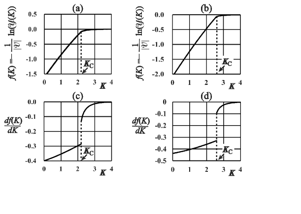
Figure 1: Free energy $f(K)=-{\frac{1}{|{\cal{V}}|}}{\ln}{\cal{Y}}(K)$ and the differentiate ${\frac{df(K)}{dK}}$ for various values of the inverse temperature $K(>0)$. They are obtained by applying the loopy belief propagation to $q$-state Potts models (55) on the square lattice with periodic boundary conditions along $x$- and $y$-directions. (a) $f(K)$ for $q=5$. (b) $f(K)$ for $q=8$. (c) ${\frac{df(K)}{dK}}$ for $q=5$. (b) ${\frac{df(K)}{dK}}$ for $q=8$. Here ${\cal{Y}}(K)$ is the partition function of the $q$-state Potts model in eq.(55), ${\cal{V}}\equiv\{1,2,{\cdots},|{\cal{V}}|\}$ is the set of all the pixels and ${\cal{E}}$ is the set of all the nearest neighbour pairs of pixels on the square lattice. The first order transition points $K_{\rm{C}}$ of the Potts model in the loopy belief propagation are $2.1972$ and $2.5871$ for $q=5$ and $q=8$, respectively.

In the present paper, we will explain, for Bayesian image segmentation, how the first order phase transitions in LBP’s for $q$-state Potts models influence EM algorithms in the maximum likelihood framework and how the inference algorithm in Ref.[30] works from the standpoint of statistical-mechanical informatics. In §2, we construct a Potts prior probability distribution for Bayesian image segmentation modeling from the standpoint of the constrained maximization of entropy. In §3, we propose a novel inference scheme, which is based on a conditional maximum likelihood framework, for estimating hyperparameters from an observed natural color image in terms of our Potts prior distribution and the LBP. In §4, we survey the inference procedure for estimating hyperparameters using the conventional maximum likelihood framework and give numerical experiments in the frameworks with the LBP. We will also clarify how the first order phase transition appears in the conventional scheme with the LBP. In §5, we give some concluding remarks.

2 Potts Prior for Probabilistic Image Segmentation

We consider an image as defined on a set of pixels arranged on a square grid graph $({\cal{V}},{\cal{E}})$, where ${\cal{V}}$ is the set of all the pixels and is defined by ${\cal{V}}{\equiv}\{i|i=1,2,{\cdots},|{\cal{V}}|\}$. There is a link $\{i,j\}$ between every nearest-neighbour pair of pixels $i$ and $j$, and ${\cal{E}}$ denotes the set of all the nearest-neighbour pairs of pixels $\{i,j\}$. The total numbers of elements in the sets ${\cal{V}}$ and ${\cal{E}}$ are denoted by $|{\cal{V}}|$ and $|{\cal{E}}|$, respectively. The goal of image segmentation is to classify the pixels into several regions. Each pixel will be assigned one of the integers ${\cal{Q}}{\equiv}\{0,1,2,{\cdots},q-1\}$ as its region label. In the present section, we give the prior probability distribution of labeled configurations on the square grid graph $({\cal{V}},{\cal{G}})$.

The label at each pixel $i$ is regarded as a random variable, denoted by $A_{i}$. Then the random field of labels is represented by ${\bm{A}}{\equiv}(A_{1},A_{2},{\cdots},A_{|{\cal{V}}|})^{\rm{T}}$, and every labeled configuration is denoted by ${\bm{a}}=(a_{1},a_{2},{\cdots},a_{|{\cal{V}}|})^{\rm{T}}$. The prior probability of a labeled configuration ${\bm{a}}$ is assumed to be specified by a constant $u$ as

$${}{\Pr}\{{\bm{A}}={\bm{a}}|u\}={\arg}{\max_{{\cal{P}}({\bm{a}})}}{\Big{\{}}-{\sum_{\bm{z}}}{\cal{P}}({\bm{z}}){\ln}{\cal{P}}({\bm{z}}){\Big{|}}$$

$${\frac{1}{|{\cal{E}}|}}{\sum_{\{i,j\}{\in}{\cal{E}}}}{\sum_{{\bm{z}}}}{\big{(}}1-{\delta}_{z_{i},z_{j}}{\big{)}}{\cal{P}}({\bm{z}})=u,{\sum_{\bm{z}}}{\cal{P}}({\bm{z}})=1{\Big{\}}},$$ (1)

where ${\bm{z}}=(z_{1},z_{2},{\cdots},z_{|{\cal{V}}|})^{\rm{T}}$ and ${\displaystyle{{\sum_{\bm{z}}}{\equiv}{\sum_{z_{1}{\in}{\cal{Q}}}}{\sum_{z_{2}{\in}{\cal{Q}}}}{\cdots}{\sum_{z_{|{\cal{V}}|}{\in}{\cal{Q}}}}}}$. By introducing the Lagrange multipliers for the constraints, we reduce the prior probability ${\Pr}\{{\bm{A}}={\bm{a}}|u\}$ to

$${\Pr}\{{\bm{A}}={\bm{a}}|u\}={\frac{1}{{\cal{Z}}(u)}}{\prod_{\{i,j\}{\in}{\cal{E}}}}{\exp}{\Big{(}}{\frac{1}{2}}{\alpha}(u){\delta}_{a_{i},a_{j}}{\Big{)}},$$ (2)

where ${\cal{Z}}(u)$ is a normalization constant. The interaction ${\alpha}(u)$ is a function of $u$ and should be determined to satisfy the following constraint condition

$${\frac{1}{|{\cal{E}}|}}{\sum_{\{i,j\}{\in}{\cal{E}}}}{\sum_{\bm{z}}}{\big{(}}1-{\delta}_{z_{i},z_{j}}{\big{)}}{\Pr}\{{\bm{A}}={\bm{z}}|u\}=u.$$ (3)

In order to calculate the estimate of the hyperparameter ${\alpha}(u)$, we have to solve the following equation:

$${\frac{1}{|{\cal{E}}|}}{\sum_{\{i,j\}{\in}{\cal{E}}}}{\sum_{{\zeta}{\in}{\cal{Q}}}}{\sum_{{\zeta}^{\prime}{\in}{\cal{Q}}}}{\big{(}}1-{\delta}_{{\zeta},{\zeta}^{\prime}}{\big{)}}{\Pr}\{A_{i}={\zeta},A_{j}={\zeta}^{\prime}|u\}=u,$$ (4)

where

$${\Pr}\{A_{i}=a_{i},A_{j}=a_{j}|u\}\equiv{\sum_{\bm{z}}}{\delta}_{z_{i},a_{i}}{\delta}_{z_{j},a_{j}}{\Pr}\{{\bm{A}}={\bm{z}}|u\}.$$ (5)

In the above mathematical framework, as shown in the deterministic equation (4) together with eqs.(2) and (5), computation of the two terms ${\sum_{\{i,j\}{\in}{\cal{E}}}}{\sum_{\bm{z}}}{\big{(}}1-{\delta}_{z_{i},z_{j}}{\big{)}}{\Pr}\{{\bm{A}}={\bm{z}}|u\}$ and ${\cal{Z}}(u)$ is critical to ${\alpha}(u)$. In LBP[9, 10, 11, 30], the marginal prior probability distributions ${\Pr}\{A_{i}=a_{i},A_{j}=a_{j}|u\}$ in eq.(5) and ${\Pr}\{A_{i}=a_{i}|u\}\equiv{\sum_{{\bm{z}}}}{\delta}_{z_{i},a_{i}}{\Pr}\{{\bm{A}}={\bm{z}}|u\}$ can be approximately reduced to

$${\Pr}\{A_{i}=a_{i},A_{j}=a_{j}|u\} \simeq {\frac{1}{{\cal{Z}}_{\{i,j\}}(u)}}{\Big{(}}{\prod_{k{\in}{\partial}i{\backslash}\{j\}}}{\lambda}_{k{\to}i}(a_{i}){\Big{)}}{\exp}{\Big{(}}{\frac{1}{2}}{\alpha}(u){\delta}_{a_{i},a_{j}}{\Big{)}}$$ (6)

$${\hskip 42.67912pt}{\times}{\Big{(}}{\prod_{k{\in}{\partial}j{\backslash}\{i\}}}{\lambda}_{k{\to}j}(a_{j}){\Big{)}}~{}(\{i,j\}{\in}{\cal{E}}),$$

$${\Pr}\{A_{i}=a_{i}|u\}\simeq{\frac{1}{{\cal{Z}}_{i}(u)}}{\prod_{k{\in}{\partial}i}}{\lambda}_{k{\to}i}(a_{i}){\hskip 5.69054pt}(i{\in}{\cal{V}}),$$ (7)

where ${\partial}i$ denotes the set of neighbouring pixels of pixel $i$. The quantities ${\cal{Z}}_{\{i,j\}}(u)$ and ${\cal{Z}}_{i}(u)$ in eqs.(6) and (7) correspond to normalization constants of approximate representations of marginal probabilities in LBP. Here $\{{\lambda}_{j{\to}i}({\xi})|i{\in}{\cal{V}},~{}j{\in}{\partial}i,~{}{\xi}{\in}{\cal{Q}}\}$ are messages in the LBP[30] for the prior probability ${\Pr}\{{\bm{A}}={\bm{a}}|u\}$ in eq.(2), and the free energy $f(u)$ per pixel in the Potts prior (2) is also approximately expressed as

$$f(u) \equiv -{\frac{1}{|{\cal{V}}|}}{\ln}{\cal{Z}}(u)$$ (8)

$${\simeq} {\frac{1}{|{\cal{V}}|}}{\Big{(}}-{\sum_{\{i,j\}{\in}{\cal{E}}}}{\ln}{\cal{Z}}_{\{i,j\}}(u)-{\sum_{i{\in}{\cal{V}}}}(1-|{\partial}i|){\ln}{\cal{Z}}_{i}(u){\Big{)}}.$$

The messages ${\lambda}_{j{\to}i}({\xi})$ (${\xi}{\in}{\cal{Q}}$, $j{\in}{\partial}i$, $i{\in}{\cal{V}}$) are determined so as to satisfy the following simultaneous equations:

$${}{\lambda}_{j{\to}i}({\xi})={\frac{{\displaystyle{{\sum_{{\zeta}{\in}{\cal{Q}}}}}}{\exp}{\Big{(}}{\frac{1}{2}}{\alpha}(u){\delta}_{{\xi},{\zeta}}{\Big{)}}{\displaystyle{{\prod_{k{\in}{\partial}j{\backslash}\{i\}}}}}{\lambda}_{k{\to}j}({\zeta})}{{\displaystyle{{\sum_{{\zeta}{\in}{\cal{Q}}}}}}{\displaystyle{{\sum_{{\zeta}^{\prime}{\in}{\cal{Q}}}}}}{\exp}{\Big{(}}{\frac{1}{2}}{\alpha}(u){\delta}_{{\zeta}^{\prime},{\zeta}}{\Big{)}}{\displaystyle{{\prod_{k{\in}{\partial}j{\backslash}\{i\}}}}}{\lambda}_{k{\to}j}({\zeta})}}$$

$${\hskip 85.35826pt}(i{\in}{\cal{V}},~{}j{\in}{\partial}i,~{}{\xi}{\in}{\cal{Q}}).$$ (9)

In Fig.2, we show the curves of ${\alpha}(u)$ and $f(u)$ along various values of $u$ for $q=5$ and $q=8$. For each fixed value of $u$, ${\alpha}(u)$ is determined so as to satisfy the constraint condition (4). The left-hand side of the constraint condition (4) is computed by using eq.(6) together with eq.(9) in LBP.

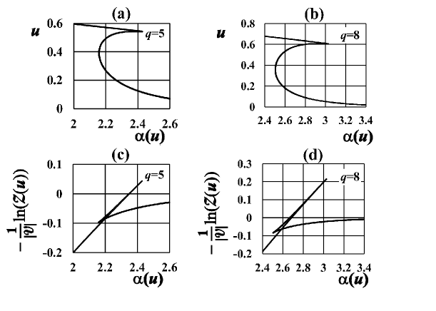
Figure 2: ${\alpha}(u)$ and $f(u)=-{\frac{1}{|{\cal{V}}|}}{\ln}{\cal{Z}}(u)$ for various values of $u$ obtained by using the loopy belief propagation of Potts models for the cases of $q=5$ and $q=8$.

3 Segmentation Algorithm for Potts Posterior and Loopy Belief Propagation

In this section, we provide a posterior probability and a hyperparameter estimation scheme in terms of the Potts prior constructed in the previous section. We combine the conditional maximization of entropy with Bayesian modeling to derive simultaneous deterministic equations for estimating hyperparameters from the given data.

The intensities of red, green, and blue channels at pixel $i$ in the observed image are regarded as random variables denoted by $D_{i}^{\rm{R}}$, $D_{i}^{\rm{G}}$ and $D_{i}^{\rm{B}}$, respectively. The random fields of red, green and blue intensities in the observed color image are then represented by the $3|{\cal{V}}|$-dimensional vector ${\bm{D}}{\equiv}({\bm{D}}_{1},{\bm{D}}_{2},{\cdots},{\bm{D}}_{|{\cal{V}}|})^{\rm{T}}$, where ${\bm{D}}_{i}\equiv(D_{i}^{\rm{R}},D_{i}^{\rm{G}},D_{i}^{\rm{B}})^{\rm{T}}$. The actual color image is denoted by ${\bm{d}}=({\bm{d}}_{1},{\bm{d}}_{2},{\cdots},{\bm{d}}_{|{\cal{V}}|})^{\rm{T}}$, where ${\bm{d}}_{i}=(d_{i}^{\rm{R}},d_{i}^{\rm{G}},d_{i}^{\rm{B}})^{\rm{T}}$. The random variables $D_{i}^{\rm{R}}$, $D_{i}^{\rm{G}}$ and $D_{i}^{\rm{B}}$ at each pixel $i$ can take any real numbers in the interval $(-{\infty},+{\infty})$. The generative process of natural color images ${\bm{d}}$ is assumed to be the following conditional probability:

$${}{\Pr}\{{\bm{D}}={\bm{d}}|{\bm{A}}={\bm{a}},{\bm{\Theta}}\}={\prod_{i{\in}{\cal{V}}}}g({\bm{d}}_{i}|a_{i},{\bm{\Theta}}),$$ (10)

where

$${\bm{\Theta}}\equiv{\Bigg{\{}}{\bm{m}}({\xi})=\left(\begin{array}[]{@{\,}ccc@{\,}}m_{\rm{R}}({\xi})\\ m_{\rm{G}}({\xi})\\ m_{\rm{B}}({\xi})\end{array}\right),{\bm{C}}({\xi})=\left(\begin{array}[]{@{\,}ccc@{\,}}C_{\rm{RR}}({\xi})&C_{\rm{GR}}({\xi})&C_{\rm{BR}}({\xi})\\ C_{\rm{RG}}({\xi})&C_{\rm{GG}}({\xi})&C_{\rm{BG}}({\xi})\\ C_{\rm{RB}}({\xi})&C_{\rm{GB}}({\xi})&C_{\rm{BB}}({\xi})\end{array}\right){\Bigg{|}}{\xi}{\in}{\cal{Q}}{\Bigg{\}}}$$ (17)

and

$${}g({\bm{d}}_{i}|a_{i},{\bm{\Theta}})\equiv{\sqrt{{\frac{1}{{\rm{det}}(2{\pi}{\bm{C}}(a_{i}))}}}}{\exp}{\Big{(}}-{\frac{1}{2}}({\bm{d}}_{i}-{\bm{m}}(a_{i}))^{\rm{T}}{\bm{C}}^{-1}(a_{i})({\bm{d}}_{i}-{\bm{m}}(a_{i})){\Big{)}}.$$ (18)

By substituting eqs.(2) and (10) into the Bayes formula, we derive the posterior probability distribution as follows:

$${\Pr}\{{\bm{A}}={\bm{a}}|{\bm{D}}={\bm{d}},u,{\bm{\Theta}}\}={\frac{1}{{\cal{Z}}({\bm{d}},u,{\bm{\Theta}})}}{\Big{(}}{\prod_{i{\in}{\cal{V}}}}g({\bm{d}}_{i}|a_{i},{\bm{\Theta}}){\Big{)}}{\Big{(}}{\prod_{\{i,j\}{\in}{\cal{E}}}}{\exp}{\big{(}}{\frac{1}{2}}{\cal{K}}{\delta}_{a_{i},a_{j}}{\big{)}}{\Big{)}},$$ (19)

where

$${\cal{Z}}({\bm{d}},u,{\bm{\Theta}})\equiv{\sum_{{\bm{z}}}}{\Big{(}}{\prod_{i{\in}{\cal{V}}}}g({\bm{d}}_{i}|a_{i},{\bm{\Theta}}){\Big{)}}{\Big{(}}{\prod_{\{i,j\}{\in}{\cal{E}}}}{\exp}{\big{(}}{\frac{1}{2}}{\cal{K}}{\delta}_{a_{i},a_{j}}{\big{)}}{\Big{)}}.$$ (20)

Another way of defining the posterior probability of a labeling ${\bm{a}}$ can be introduced through the following definition:

$${}{\Pr}\{{\bm{A}}={\bm{a}}|{\bm{D}}={\bm{d}},u,{\bm{\Theta}}\}={\frac{{\Big{(}}{\displaystyle{{\prod_{i{\in}V}}}}{\sqrt{{\frac{1}{{\rm{det}}(2{\pi}{\bm{C}}(a_{i}))}}}}{\Big{)}}{\widehat{{\cal{P}}}}({\bm{a}})}{{\displaystyle{{\sum_{{\bm{z}}}}}}{\Big{(}}{\displaystyle{{\prod_{i{\in}V}}}}{\sqrt{{\frac{1}{{\rm{det}}(2{\pi}{\bm{C}}(z_{i}))}}}}{\Big{)}}{\widehat{{\cal{P}}}}({\bm{z}})}}$$ (21)

$${}{\widehat{{\cal{P}}}}({\bm{a}})={\arg}{\max_{{\cal{P}}({\bm{a}})}}{\Big{\{}}-{\sum_{\bm{z}}}{\cal{P}}({\bm{z}}){\ln}{\cal{P}}({\bm{z}}){\Big{|}}{\sum_{\bm{z}}}{\cal{P}}({\bm{z}})=1,{\sum_{\{i,j\}{\in}{\cal{E}}}}{\sum_{\bm{z}}}{\big{(}}1-{\delta}_{z_{i},z_{j}}{\big{)}}{\cal{P}}({\bm{z}})=u,$$

$${}{\sum_{i{\in}{\cal{V}}}}{\bm{d}}_{i}{\sum_{\bm{z}}}{\delta}_{z_{i},{\xi}}{\cal{P}}({\bm{z}})={\sum_{i{\in}{\cal{V}}}}{\bm{m}}({\xi}){\sum_{\bm{z}}}{\delta}_{z_{i},{\xi}}{\cal{P}}({\bm{z}})~{}({\xi}{\in}{\cal{Q}}),$$

$${}{\sum_{i{\in}{\cal{V}}}}{\bm{d}}_{i}{\bm{d}}_{i}^{\rm{T}}{\displaystyle{{\sum_{\bm{z}}}}}{\delta}_{z_{i},{\xi}}{\cal{P}}({\bm{z}})={\sum_{i{\in}{\cal{V}}}}{\big{(}}{\bm{C}}({\xi})+{\bm{m}}({\xi}){\bm{m}}^{\rm{T}}({\xi}){\big{)}}{\displaystyle{{\sum_{\bm{z}}}}}{\delta}_{z_{i},{\xi}}{\cal{P}}({\bm{z}})~{}({\xi}{\in}{\cal{Q}}){\Big{\}}}.$$ (22)

By introducing Lagrange multipliers ${\Lambda}_{0}$, ${\Lambda}_{1}$, ${\bm{\Lambda}}_{2}({\xi})=\left(\begin{array}[]{@{\,}ccc@{\,}}{\Lambda}_{2}^{\rm{R}}({\xi})\\ {\Lambda}_{2}^{\rm{G}}({\xi})\\ {\Lambda}_{2}^{\rm{B}}({\xi})\end{array}\right)$ (${\xi}{\in}{\cal{Q}}$) and ${\bm{\Lambda}}_{3}({\xi})=\left(\begin{array}[]{@{\,}ccc@{\,}}\footnotesize{\Lambda}_{3}^{\rm{RR}}({\xi})&{\Lambda}_{3}^{\rm{GR}}({\xi})&{\Lambda}_{3}^{\rm{BR}}({\xi})\\ {\Lambda}_{3}^{\rm{RG}}({\xi})&{\Lambda}_{3}^{\rm{GG}}({\xi})&{\Lambda}_{3}^{\rm{BG}}({\xi})\\ {\Lambda}_{3}^{\rm{RB}}({\xi})&{\Lambda}_{3}^{\rm{GB}}({\xi})&{\Lambda}_{3}^{\rm{BB}}({\xi})\end{array}\right)$ (${\xi}{\in}{\cal{Q}}$) for the constraints and by considering the extremum condition with respect to ${\cal{P}}({\bm{a}})$, the right-hand side of eq.(22) is reduced to the following expression:

$${\cal{P}}({\bm{a}}) \propto {\Big{(}}{\prod_{\{i,j\}{\in}{\cal{E}}}}{\exp}{\big{(}}-{\Lambda}_{1}(1-{\delta}_{a_{i},a_{j}}){\big{)}}{\Big{)}}$$ (23)

$${}{\times}{\Bigg{(}}{\prod_{i{\in}{\cal{V}}}}{\exp}{\Big{(}}-{\bm{d}}_{i}^{\rm{T}}{\bm{{\Lambda}}}_{3}(a_{i}){\bm{d}}_{i}-{\frac{1}{2}}{\bm{d}}_{i}^{\rm{T}}{\bm{{\Lambda}}}_{2}(a_{i})-{\frac{1}{2}}{\bm{{\Lambda}}}_{2}^{\rm{T}}(a_{i}){\bm{d}}_{i}^{\rm{T}}{\Big{)}}$$

$${}{\times}{\exp}{\Big{(}}{\bm{m}}^{\rm{T}}(a_{i}){\bm{{\Lambda}}}_{3}(a_{i}){\bm{m}}(a_{i})+{\frac{1}{2}}{\bm{{\Lambda}}}_{2}^{\rm{T}}(a_{i}){\bm{m}}(a_{i})+{\frac{1}{2}}{\bm{m}}^{\rm{T}}(a_{i}){\bm{{\Lambda}}}_{2}(a_{i}){\Big{)}}$$

$${}{\times}{\exp}{\Big{(}}{\sum_{{\kappa}{\in}\{{\rm{R}},{\rm{G}},{\rm{B}}\}}}{\sum_{{\kappa}^{\prime}{\in}\{{\rm{R}},{\rm{G}},{\rm{B}}\}}}C_{{\kappa},{\kappa}^{\prime}}(a_{i}){\Lambda}_{3}^{{\kappa},{\kappa}^{\prime}}(a_{i}){\Big{)}}{\Bigg{)}},$$

up to the normalization constant including ${\Lambda}_{0}$. The Lagrange multipliers ${\Lambda}_{1}$, ${\bm{{\Lambda}}}_{3}({\xi})$ (${\xi}{\in}{\cal{Q}}$) and ${\bm{{\Lambda}}}_{2}({\xi})$ (${\xi}{\in}{\cal{Q}}$) are determined so as to satisfy the constraint conditions:

$${\frac{1}{|{\cal{E}}|}}{\displaystyle{{\sum_{\{i,j\}{\in}{\cal{E}}}}}}{\displaystyle{{\sum_{\bm{z}}}}}{\big{(}}1-{\delta}_{z_{i},z_{j}}{\big{)}}{\cal{P}}({\bm{z}})=u,$$ (24)

$${\frac{{\displaystyle{{\sum_{i{\in}{\cal{V}}}}}}{\bm{d}}_{i}{\displaystyle{{\sum_{\bm{z}}}}}{\delta}_{z_{i},{\xi}}{\cal{P}}({\bm{z}})}{{\displaystyle{{\sum_{i{\in}{\cal{V}}}}}}{\displaystyle{{\sum_{\bm{z}}}}}{\delta}_{z_{i},{\xi}}{\cal{P}}({\bm{z}})}}={\bm{m}}({\xi})~{}({\xi}{\in}{\cal{Q}}),$$ (25)

$${\frac{{\displaystyle{{\sum_{i{\in}{\cal{V}}}}}}{\big{(}}{\bm{d}}_{i}-{\bm{m}}({\xi}){\big{)}}{\big{(}}{\bm{d}}_{i}-{\bm{m}}({\xi}){\big{)}}^{\rm{T}}{\displaystyle{{\sum_{\bm{z}}}}}{\delta}_{z_{i},{\xi}}{\cal{P}}({\bm{z}})}{{\displaystyle{{\sum_{i{\in}{\cal{V}}}}}}{\displaystyle{{\sum_{\bm{z}}}}}{\delta}_{z_{i},{\xi}}{\cal{P}}({\bm{z}})}}={\bm{C}}({\xi})~{}({\xi}{\in}{\cal{Q}}).$$ (26)

Moreover, in order to ensure eq.(23) as an identity with respect to every label configuration of ${\bm{a}}$, we have to impose the following equalities:

$${\Lambda}_{1}={\frac{1}{2}}{\alpha}(u),~{}({\xi}{\in}{\cal{Q}}),$$ (27)

$${\bm{\Lambda}}_{2}({\xi})=-{\bm{C}}^{-1}({\xi}){\bm{m}}({\xi})~{}({\xi}{\in}{\cal{Q}}),$$ (28)

$${{\bm{{\Lambda}}}_{3}}({\xi})={\frac{1}{2}}{\bm{C}}^{-1}({\xi})~{}({\xi}{\in}{\cal{Q}}),$$ (29)

as sufficient conditions for eq.(21) with respect to the right-hand sides of equations (19) and (23). Because ${\bm{C}}({\xi})$ (${\xi}{\in}{\cal{Q}}$) are symmetric matrices, we can show that ${\displaystyle{{\sum_{{\kappa}{\in}\{{\rm{R}},{\rm{G}},{\rm{B}}\}}}}}{\displaystyle{{\sum_{{\kappa}^{\prime}{\in}\{{\rm{R}},{\rm{G}},{\rm{B}}\}}}}}C_{{\kappa},{\kappa}^{\prime}}({\xi}){\Lambda}_{3}^{{\kappa},{\kappa}^{\prime}}({\xi})={\frac{3}{2}}$ (${\xi}{\in}{\cal{Q}}$) in eq.(23) by using eq.(29). By combining the above arguments (19), (23), (24)-(26), and (27)-(28) with the ones in eq.(2) and eq.(3), the simultaneous deterministic equations of estimates ${\widehat{u}}({\bm{d}})$ and ${\widehat{\bm{\Theta}}}({\bm{d}})=\{{\widehat{\bm{m}}}({\xi},{\bm{d}}),{\widehat{\bm{C}}}({\xi},{\bm{d}})|{\xi}{\in}{\cal{Q}}\}$ of $u$ and ${\bm{\Theta}}$ should then be reduced to the following constraints:

$${}{\frac{1}{|{\cal{E}}|}}{\sum_{\{i,j\}{\in}{\cal{E}}}}{\sum_{{\zeta}{\in}{\cal{Q}}}}{\sum_{{\zeta}^{\prime}{\in}{\cal{Q}}}}{\big{(}}1-{\delta}_{{\zeta},{\zeta}^{\prime}}{\big{)}}{\Pr}\{A_{i}={\zeta},A_{j}={\zeta}^{\prime}|{\bm{D}}={\bm{d}},{\widehat{u}}({\bm{d}}),{\widehat{\bm{\Theta}}}({\bm{d}})\}$$ (30)

$$= {\frac{1}{|{\cal{E}}|}}{\sum_{\{i,j\}{\in}{\cal{E}}}}{\sum_{{\zeta}{\in}{\cal{Q}}}}{\sum_{{\zeta}^{\prime}{\in}{\cal{Q}}}}{\big{(}}1-{\delta}_{{\zeta},{\zeta}^{\prime}}{\big{)}}{\Pr}\{A_{i}={\zeta},A_{j}={\zeta}^{\prime}|{\widehat{u}}({\bm{d}})\},$$

$${}{\frac{{\displaystyle{{\sum_{i{\in}{\cal{V}}}}}}{\bm{d}}_{i}{\Pr}\{A_{i}={\xi}|{\bm{D}}={\bm{d}},{\widehat{u}}({\bm{d}}),{\widehat{\bm{\Theta}}}({\bm{d}})\}}{{\displaystyle{{\sum_{i{\in}{\cal{V}}}}}}{\Pr}\{A_{i}={\xi}|{\bm{D}}={\bm{d}},{\widehat{u}}({\bm{d}}),{\widehat{\bm{\Theta}}}({\bm{d}})\}}}={\widehat{\bm{m}}}({\xi},{\bm{d}})~{}({\xi}{\in}{\cal{Q}}),$$ (31)

$${}{\frac{{\displaystyle{{\sum_{i{\in}{\cal{V}}}}}}{\big{(}}{\bm{d}}_{i}-{\widehat{\bm{m}}}({\xi},{\bm{d}}){\big{)}}{\big{(}}{\bm{d}}_{i}-{\widehat{\bm{m}}}({\xi},{\bm{d}}){\big{)}}^{\rm{T}}{\Pr}\{A_{i}={\xi}|{\bm{D}}={\bm{d}},{\widehat{u}}({\bm{d}}),{\widehat{\bm{\Theta}}}({\bm{d}})\}}{{\displaystyle{{\sum_{i{\in}{\cal{V}}}}}}{\Pr}\{A_{i}={\xi}|{\bm{D}}={\bm{d}},{\widehat{u}}({\bm{d}}),{\widehat{\bm{\Theta}}}({\bm{d}})\}}}$$

$${\hskip 199.16928pt}={\widehat{\bm{C}}}({\xi},{\bm{d}})~{}({\xi}{\in}{\cal{Q}}),$$ (32)

where

$${\Pr}\{A_{i}=a_{i},A_{j}=a_{j}|{\bm{D}}={\bm{d}},u,{\bm{\Theta}}\}\equiv{\sum_{\bm{z}}}{\delta}_{z_{i},a_{i}}{\delta}_{z_{j},a_{j}}{\Pr}\{{\bm{A}}={\bm{z}}|{\bm{D}}={\bm{d}},u,{\bm{\Theta}}\},$$ (33)

$${\Pr}\{A_{i}=a_{i}|{\bm{D}}={\bm{d}},u,{\bm{\Theta}}\}\equiv{\sum_{\bm{z}}}{\delta}_{z_{i},a_{i}}{\Pr}\{{\bm{A}}={\bm{z}}|{\bm{D}}={\bm{d}},u,{\bm{\Theta}}\}.$$ (34)

Given the estimates ${\widehat{u}}$ and ${\widehat{\bm{\Theta}}}$, the estimate of labeling ${\widehat{\bm{a}}}({\bm{d}})=({\widehat{a}}_{1}({\bm{d}}),{\widehat{a}}_{2}({\bm{d}}),{\cdots},{\widehat{a}}_{|{\cal{V}}|}({\bm{d}}))^{\rm{T}}$ is determined by

$${\widehat{a}}_{i}({\bm{d}})\equiv{\max_{{\zeta}{\in}{\cal{Q}}}}{\Pr}\{A_{i}={\zeta}|{\bm{D}}={\bm{d}},{\widehat{u}}({\bm{d}}),{\widehat{\bm{\Theta}}}({\bm{d}})\}{\hskip 5.69054pt}(i{\in}{\cal{V}}).$$ (35)

The above method of producing the labeling is called maximum posterior marginal (MPM) estimation.

In LBP, the marginal probability distributions ${\Pr}\{A_{i}=a_{i},A_{j}=a_{j}|{\bm{D}}={\bm{d}},u,{\bm{\Theta}}\}$ and ${\Pr}\{A_{i}=a_{i}|{\bm{D}}={\bm{d}},u,{\bm{\Theta}}\}$ can be approximately reduced to

$${\Pr}\{A_{i}=a_{i},A_{j}=a_{j}|{\bm{D}}={\bm{d}},u,{\bm{\Theta}}\} \simeq {\frac{1}{{\cal{Z}}_{\{i,j\}}({\bm{d}},u,{\bm{\Theta}})}}{\Big{(}}{\prod_{k{\in}{\partial}i{\backslash}\{j\}}}{\mu}_{k{\to}i}(a_{i}){\Big{)}}$$ (36)

$${}{\times}g({\bm{d}}_{i}|a_{i},{\bm{\Theta}}){\exp}{\big{(}}{\frac{1}{2}}{\alpha}(u){\delta}_{a_{i},a_{j}}{\big{)}}g({\bm{d}}_{j}|a_{j},{\bm{\Theta}}){\Big{(}}{\prod_{k{\in}{\partial}j{\backslash}\{i\}}}{\mu}_{k{\to}j}(a_{j}){\Big{)}}{\hskip 5.69054pt}(\{i,j\}{\in}{\cal{E}}),$$

$${\Pr}\{A_{i}=a_{i}|{\bm{D}}={\bm{d}},u,{\bm{\Theta}}\} \simeq {\frac{1}{{\cal{Z}}_{i}({\bm{d}},u,{\bm{\Theta}})}}g({\bm{d}}_{i}|a_{i},{\bm{\Theta}}){\Big{(}}{\prod_{k{\in}{\partial}i}}{\mu}_{k{\to}i}(a_{i}){\Big{)}}{\hskip 5.69054pt}(i{\in}{\cal{V}}).$$ (37)

The quantities ${\cal{Z}}_{\{i,j\}}({\bm{d}},u,{\bm{\Theta}})$ and ${\cal{Z}}_{i}({\bm{d}},u,{\bm{\Theta}})$ in eqs.(36) and (37) correspond to normalization constants of approximate representation to marginal probabilities in LBP. Here $\{{\mu}_{j{\to}i}({\xi})|i{\in}{\cal{V}},~{}j{\in}{\partial}i,~{}{\xi}{\in}{\cal{Q}}\}$ are messages in the LBP[30] for the posterior probabilities ${\Pr}\{{\bm{A}}={\bm{a}}|{\bm{D}}={\bm{d}},u,{\bm{\Theta}}\}$ in eq.(19). They are determined so as to satisfy the following simultaneous fixed-point equations:

$${\mu}_{j{\to}i}({\xi}) = {\frac{{\displaystyle{{\sum_{{\zeta}{\in}{\cal{Q}}}}}}{\exp}{\big{(}}{\frac{1}{2}}{\alpha}(u){\delta}_{{\xi},{\zeta}}{\big{)}}g({\bm{d}}_{j}|{\zeta},{\bm{\Theta}}){\displaystyle{{\prod_{k{\in}{\partial}j{\backslash}\{i\}}}}}{\mu}_{k{\to}j}({\zeta})}{{\displaystyle{{\sum_{{\zeta}{\in}{\cal{Q}}}}}}{\displaystyle{{\sum_{{\zeta}^{\prime}{\in}{\cal{Q}}}}}}{\exp}{\big{(}}{\frac{1}{2}}{\alpha}(u){\delta}_{{\zeta}^{\prime},{\zeta}}{\big{)}}g({\bm{d}}_{j}|{\zeta},{\bm{\Theta}}){\displaystyle{{\prod_{k{\in}{\partial}j{\backslash}\{i\}}}}}{\mu}_{k{\to}j}({\zeta})}}$$ (38)

$${\hskip 85.35826pt}(i{\in}{\cal{V}},j{\in}{\partial}i,{\xi}{\in}{\cal{Q}}).$$

Here ${\partial}i$ denotes the pixels that are neighbours of pixel $i$. The left-hand sides in eqs.(30), (31) and (32) can be computed by means of eqs.(36), (37), and (38).

The practical segmentation algorithm for an observed image ${\bm{d}}$ is summarized as follows:

    Inference Algorithm for ${\widehat{u}}({\bm{d}})$, ${\alpha}{\big{(}}{\widehat{u}}({\bm{d}}){\big{)}}$ and ${\widehat{\bm{\Theta}}}({\bm{d}})$

     Step 1

Input the data ${\bm{d}}$. Set initial values for $u$, ${\cal{K}}$, ${\bm{\Theta}}{\equiv}\{{\bm{m}}({\zeta}),{\bm{C}}({\zeta})|{\zeta}{\in}{\cal{Q}}\}$ and $\{{\widehat{\mu}}_{j{\to}i}({\xi})|i{\in}{\cal{V}},j{\in}{\partial}i,{\xi}{\in}{\cal{Q}}\}$, and $t\leftarrow 0$.

     Step 2

Set initial values for $\{{\widehat{\lambda}}_{j{\to}i}({\xi})|i{\in}{\cal{V}},j{\in}{\partial}i,{\xi}{\in}{\cal{Q}}\}$ and repeat the following update rules until ${\cal{K}}$ and $\{{\widehat{\lambda}}_{j{\to}i}({\xi})|i{\in}{\cal{V}},j{\in}{\partial}i,{\xi}{\in}{\cal{Q}}\}$ converge:

$${\lambda}_{j{\to}i}({\xi}) \leftarrow {\frac{{\displaystyle{{\sum_{{\zeta}{\in}{\cal{Q}}}}}}{\exp}{\big{(}}{\frac{1}{2}}{\cal{K}}{\delta}_{{\xi},{\zeta}}{\big{)}}{\displaystyle{{\prod_{k{\in}{\partial}j{\backslash}\{i\}}}}}{\widehat{\lambda}}_{k{\to}j}({\zeta})}{{\displaystyle{{\sum_{{\zeta}{\in}{\cal{Q}}}}}}{\displaystyle{{\sum_{{\zeta}^{\prime}{\in}{\cal{Q}}}}}}{\exp}{\big{(}}{\frac{1}{2}}{\cal{K}}{\delta}_{{\zeta}^{\prime},{\zeta}}{\big{)}}{\displaystyle{{\prod_{k{\in}{\partial}j{\backslash}\{i\}}}}}{\widehat{\lambda}}_{k{\to}j}({\zeta})}}$$ (39)

$${\hskip 85.35826pt}({\xi}{\in}{\cal{Q}},~{}i{\in}{\cal{V}},~{}j{\in}{\partial}i),$$

$${}{\cal{A}}_{i}\leftarrow{\displaystyle{{\sum_{{\zeta}{\in}{\cal{Q}}}}}}{\prod_{k{\in}{\partial}i}}{\lambda}_{k{\to}i}({\zeta}){\hskip 5.69054pt}(i{\in}{\cal{V}}),$$ (40)

$${}{\cal{A}}_{\{i,j\}}\leftarrow{\displaystyle{{\sum_{{\zeta}{\in}{\cal{Q}}}}}}{\displaystyle{{\sum_{{\zeta}^{\prime}{\in}{\cal{Q}}}}}}{\Big{(}}{\prod_{k{\in}{\partial}i{\backslash}\{j\}}}{\lambda}_{k{\to}i}({\zeta}){\Big{)}}{\exp}{\Big{(}}{\frac{1}{2}}{\cal{K}}{\delta}_{{\zeta},{\zeta}^{\prime}}{\Big{)}}$$

$${\hskip 28.45274pt}{\times}{\Big{(}}{\prod_{k{\in}{\partial}j{\backslash}\{i\}}}{\lambda}_{k{\to}j}({\zeta}^{\prime}){\Big{)}}~{}(\{i,j\}{\in}{\cal{E}}),$$ (41)

$${\cal{K}} \leftarrow {\cal{K}}{\times}{\Bigg{(}}{\frac{1}{u|{\cal{E}}|}}{\sum_{\{i,j\}{\in}{\cal{E}}}}{\frac{1}{{\cal{A}}_{\{i,j\}}}}{\displaystyle{{\sum_{{\zeta}{\in}{\cal{Q}}}}}}{\displaystyle{{\sum_{{\zeta}^{\prime}{\in}{\cal{Q}}}}}}{\big{(}}1-{\delta}_{{\zeta},{\zeta}^{\prime}}{\big{)}}$$ (42)

$${\hskip 28.45274pt}{\times}{\Big{(}}{\prod_{k{\in}{\partial}i{\backslash}\{j\}}}{\lambda}_{k{\to}i}({\zeta}){\Big{)}}{\exp}{\Big{(}}{\frac{1}{2}}{\cal{K}}{\delta}_{{\zeta},{\zeta}^{\prime}}{\Big{)}}{\Big{(}}{\prod_{k{\in}{\partial}j{\backslash}\{i\}}}{\lambda}_{k{\to}j}({\zeta}^{\prime}){\Big{)}}{\Bigg{)}}^{1/4}.$$

$${\widehat{\lambda}}_{j{\to}i}({\xi}) \leftarrow {\lambda}_{j{\to}i}({\xi})~{}({\xi}{\in}{\cal{Q}},~{}i{\in}{\cal{V}},~{}j{\in}{\partial}i).$$ (43)

     Step 3

Update ${\bm{\Theta}}$, $\{{\mu}_{j{\to}i}({\xi})|{\xi}{\in}{\cal{Q}},i{\in}{\cal{V}},j{\in}{\partial}i\}$ and $u$ according to the following rules:

$${\mu}_{j{\to}i}({\xi}) \leftarrow {\frac{{\displaystyle{{\sum_{{\zeta}{\in}{\cal{Q}}}}}}{\exp}{\big{(}}{\frac{1}{2}}{\alpha}(u){\delta}_{{\xi},{\zeta}}{\big{)}}g({\bm{d}}_{j}|{\zeta},{\bm{\Theta}}){\displaystyle{{\prod_{k{\in}{\partial}j{\backslash}\{i\}}}}}{\widehat{\mu}}_{k{\to}j}({\zeta})}{{\displaystyle{{\sum_{{\zeta}{\in}{\cal{Q}}}}}}{\displaystyle{{\sum_{{\zeta}^{\prime}{\in}{\cal{Q}}}}}}{\exp}{\big{(}}{\frac{1}{2}}{\alpha}(u){\delta}_{{\zeta}^{\prime},{\zeta}}{\big{)}}g({\bm{d}}_{j}|{\zeta},{\bm{\Theta}}){\displaystyle{{\prod_{k{\in}{\partial}j{\backslash}\{i\}}}}}{\widehat{\mu}}_{k{\to}j}({\zeta})}}$$ (44)

$${\hskip 85.35826pt}({\xi}{\in}{\cal{Q}},i{\in}{\cal{V}},j{\in}{\partial}i),$$

$${\cal{B}}_{i} \leftarrow {\displaystyle{{\sum_{{\zeta}{\in}{\cal{Q}}}}}}g({\bm{d}}_{i}|{\zeta},{\bm{\Theta}}){\prod_{k{\in}{\partial}i}}{\mu}_{k{\to}i}({\zeta}){\hskip 5.69054pt}(i{\in}{\cal{V}}),$$ (45)

$${\cal{B}}_{\{i,j\}} \leftarrow {\displaystyle{{\sum_{{\zeta}{\in}{\cal{Q}}}}}}{\displaystyle{{\sum_{{\zeta}^{\prime}{\in}{\cal{Q}}}}}}{\Big{(}}{\prod_{k{\in}{\partial}i{\backslash}\{j\}}}{\mu}_{k{\to}i}({\zeta}){\Big{)}}g({\bm{d}}_{i}|{\zeta},{\bm{\Theta}}){\exp}{\big{(}}{\frac{1}{2}}{\alpha}(u){\delta}_{{\zeta},{\zeta}^{\prime}}{\big{)}}$$ (46)

$${\hskip 28.45274pt}{\times}g({\bm{d}}_{j}|{\zeta}^{\prime},{\bm{\Theta}}){\Big{(}}{\prod_{k{\in}{\partial}j{\backslash}\{i\}}}{\mu}_{k{\to}j}({\zeta}^{\prime}){\Big{)}}~{}(\{i,j\}{\in}{\cal{E}}),$$

$${\bm{m}}({\xi}) \leftarrow {\frac{{\displaystyle{{\sum_{i{\in}{\cal{V}}}}}}{\displaystyle{{\frac{1}{{\cal{B}}_{i}}}}}{\bm{d}}_{i}g({\bm{d}}_{i}|{\xi},{\bm{\Theta}}){\Big{(}}{\displaystyle{{\prod_{k{\in}{\partial}i}}}}{\mu}_{k{\to}i}({\xi}){\Big{)}}}{{\displaystyle{{\sum_{i{\in}{\cal{V}}}}}}{\displaystyle{{\frac{1}{{\cal{B}}_{i}}}}}g({\bm{d}}_{i}|{\xi},{\bm{\Theta}}){\Big{(}}{\displaystyle{{\prod_{k{\in}{\partial}i}}}}{\mu}_{k{\to}i}({\xi}){\Big{)}}}},$$ (47)

$${\bm{C}}({\xi}) \leftarrow {\frac{{\displaystyle{{\sum_{i{\in}{\cal{V}}}}}}{\displaystyle{{\frac{1}{{\cal{B}}_{i}}}}}{\big{(}}{\bm{d}}_{i}-{\bm{m}}({\xi}){\big{)}}{\big{(}}{\bm{d}}_{i}-{\bm{m}}({\xi}){\big{)}}^{\rm{T}}g({\bm{d}}_{i}|{\xi},{\bm{\Theta}}){\Big{(}}{\displaystyle{{\prod_{k{\in}{\partial}i}}}}{\mu}_{k{\to}i}({\xi}){\Big{)}}}{{\displaystyle{{\sum_{i{\in}{\cal{V}}}}}}{\displaystyle{{\frac{1}{{\cal{B}}_{i}}}}}g({\bm{d}}_{i}|{\xi},{\bm{\Theta}}){\Big{(}}{\displaystyle{{\prod_{k{\in}{\partial}i}}}}{\mu}_{k{\to}i}({\xi}){\Big{)}}}},$$ (48)

$${\bm{\Theta}} \leftarrow \{{\bm{m}}({\xi}),{\bm{C}}({\xi})|{\xi}{\in}{\cal{Q}}\},$$ (49)

$$u \leftarrow {\frac{1}{|{\cal{E}}|}}{\sum_{\{i,j\}{\in}{\cal{E}}}}{\Bigg{(}}{\frac{1}{{\cal{B}}_{\{i,j\}}}}{\displaystyle{{\sum_{{\zeta}{\in}{\cal{Q}}}}}}{\displaystyle{{\sum_{{\zeta}^{\prime}{\in}{\cal{Q}}}}}}{\big{(}}1-{\delta}_{{\zeta},{\zeta}^{\prime}}{\big{)}}{\Big{(}}{\prod_{k{\in}{\partial}i{\backslash}\{j\}}}{\mu}_{k{\to}i}({\zeta}){\Big{)}}$$ (50)

$${\hskip 28.45274pt}{\times}g({\bm{d}}_{i}|{\zeta},{\bm{\Theta}}){\exp}{\big{(}}{\frac{1}{2}}{\alpha}(u){\delta}_{{\zeta},{\zeta}^{\prime}}{\big{)}}g({\bm{d}}_{j}|{\zeta}^{\prime},{\bm{\Theta}}){\Big{(}}{\prod_{k{\in}{\partial}j{\backslash}\{i\}}}{\mu}_{k{\to}j}({\zeta}^{\prime}){\Big{)}}{\Bigg{)}}.$$

$${\widehat{\mu}}_{j{\to}i}({\xi}) \leftarrow {\mu}_{j{\to}i}({\xi})~{}({\xi}{\in}{\cal{Q}},~{}i{\in}{\cal{V}},~{}j{\in}{\partial}i).$$ (51)

     Step 4

Output the following quantities:

$$t\leftarrow t+1,{\hskip 5.69054pt}{\widehat{u}}({\bm{d}}){\leftarrow}u,{\hskip 5.69054pt}{\alpha}({\widehat{u}}({\bm{d}})){\leftarrow}{\cal{K}},$$ (52)

$${\widehat{\bm{\Theta}}}({\bm{d}})\equiv\{{\widehat{\bm{m}}}({\xi},{\bm{d}}),{\widehat{\bm{C}}}({\xi},{\bm{d}})|{\xi}{\in}{\cal{Q}}\}\leftarrow{\bm{\Theta}},$$ (53)

$${\widehat{a}}_{i}({\bm{d}})\leftarrow{\arg}{\max_{{\zeta}{\in}{\cal{Q}}}}g({\bm{d}}_{i}|{\zeta},{\bm{\Theta}}){\prod_{k{\in}{\partial}i}}{\mu}_{k{\to}i}({\zeta}){\hskip 5.69054pt}(i{\in}{\cal{V}}),$$ (54)

and stop if ${\widehat{u}}({\bm{d}})$ and ${\widehat{\bm{\Theta}}}({\bm{d}})$ converge. Go to Step 2 otherwise.

We use six test images, as shown in Figs.3(a)-(f), where three images are from the Berkeley Segmentation Data Set 500 (BSDS500)[31, 32] and the other three images are from the image database of Signal and Image Processing Institute, University of Southern California (SPIP-USC)[33] to demonstrate the effectiveness of our method. The processes of the proposed hyperparameter estimation for the images in Fig.3(a)-(f) are plotted in Figs.4(a)-(f) and 5(a)-(f) under $q=5$ and $q=8$, respectively. The solid circles in Figs.4 and 5 correspond to $({\alpha}({\widehat{u}}({\bm{d}})),{\widehat{u}}({\bm{d}}))$ in Step 4, and the solid lines are ${\alpha}(u)$ for various values of $u$ and are also given in Fig.2. In Table 1, we show the estimates ${\widehat{u}}({\bm{d}})$ and ${\alpha}({\widehat{u}}({\bm{d}}))$ in the cases of $q=5$ and $q=8$ for the images ${\bm{d}}$ in Fig.3. The segmentation results for the test images ${\bm{d}}$ in Fig.3 are shown in Figs.6 and 7 for $q=5$ and $q=8$, where the results are represented as color images ${\Big{(}}{\widehat{\bm{m}}}{\big{(}}{\widehat{a}}_{1}({\bm{d}}),{\bm{d}}{\big{)}},{\cdots},{\widehat{\bm{m}}}{\big{(}}{\widehat{a}}_{|{\cal{V}}|}({\bm{d}}),{\bm{d}}{\big{)}}{\Big{)}}^{\rm{T}}$ in terms of the average vectors ${\bm{m}}({\xi},{\bm{d}})$ (${\xi}{\in}{\cal{Q}}$) and the estimate of labeling ${\widehat{a}}({\bm{d}})$.

(a)                                       (b)

(c)                                       (d)

(e)                                       (f)

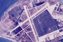
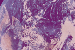
Figure 3: (a)-(c) Three test images in the Berkeley Segmentation Data Set 500 (BSDS500)[31, 32]. (d)-(f) Three test images from the database of Signal and Image Processing Institute, University of Southern California (SPIP-USC)[33]. Each color image is represented by ${\bm{d}}=({\bm{d}}_{1},{\bm{d}}_{2},{\cdots},{\bm{d}}_{|{\cal{V}}|})^{\rm{T}}$, where ${\bm{d}}_{i}=(d_{i}^{\rm{R}},d_{i}^{\rm{G}},d_{i}^{\rm{B}})^{\rm{T}}$

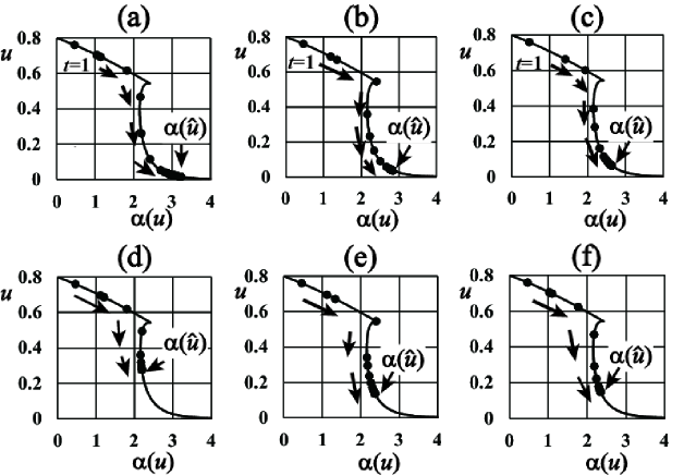
Figure 4: Hyperparameter estimation process by using our proposed inference algorithm of §3 for $q=5$. The solid circles in (a)-(f) are $({\alpha}({\widehat{u}}({\bm{d}})),{\widehat{u}}({\bm{d}}))$ at $t=1,2,3,{\cdots}$ in Step 4 for the images ${\bm{d}}$ in Fig.3(a)-(f), respectively. Our estimation process in the proposed inference algorithm almost converges within $t\geq 30$ for each ${\bm{d}}$. The solid lines are ${\alpha}(u)$ for various values of $u$ and are also given in Fig.2(a).

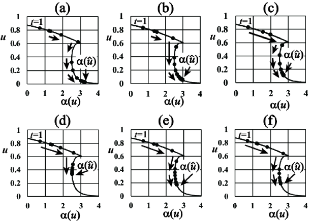
Figure 5: Hyperparameter estimation process by using our proposed inference algorithm in §3 for $q=8$. The solid circles in (a)-(f) are $({\alpha}({\widehat{u}}({\bm{d}})),{\widehat{u}}({\bm{d}}))$ at $t=1,2,3,{\cdots}$ in Step 4 for the images ${\bm{d}}$ in Fig.3(a)-(f), respectively. Our estimation process in the proposed inference algorithm almost converges within $t\geq 30$ for each ${\bm{d}}$. The solid lines are ${\alpha}(u)$ for various values of $u$ and are also given in Fig.2(b).

(a)                                       (b)

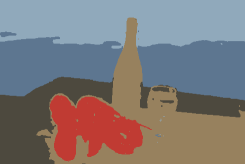
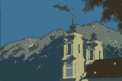
(c)                                       (d)

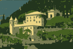
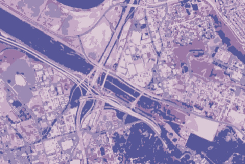
(e)                                       (f)

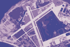
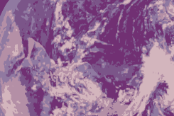
Figure 6: Segmentation ${\bm{\widehat{a}}}({\bm{d}})={\big{(}}{\widehat{a}}_{1}({\bm{d}}),{\widehat{a}}_{2}({\bm{d}}),{\cdots},{\widehat{a}}_{|{\cal{V}}|}({\bm{d}}){\big{)}}^{\rm{T}}$ by using the proposed algorithm based on our conditional maximum entropy framework and the loopy belief propagation of §3 in the case of $q=5$. The results in (a)-(f) are shown with the color ${\widehat{\bm{m}}}{\big{(}}{\widehat{a}}_{i}({\bm{d}}),{\bm{d}}{\big{)}}$ at each pixel $i$ for the observed images ${\bm{d}}$ in Fig.3.

(a)                                       (b)

(c)                                       (d)

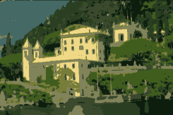
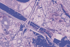
(e)                                       (f)

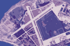
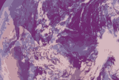
Figure 7: Segmentation ${\bm{\widehat{a}}}({\bm{d}})={\big{(}}{\widehat{a}}_{1}({\bm{d}}),{\widehat{a}}_{2}({\bm{d}}),{\cdots},{\widehat{a}}_{|{\cal{V}}|}({\bm{d}}){\big{)}}^{\rm{T}}$ by using the proposed algorithm based on our conditional maximum entropy framework and the loopy belief propagation of §3 in the case of $q=8$. The results in (a)-(f) are shown for the observed images ${\bm{d}}$ in Fig.3.

Table 1: Estimates of hyperparameters ${\widehat{u}}({\bm{d}})$ and ${\alpha}({\widehat{u}}({\bm{d}}))$ by using the proposed algorithm described in section 3 for each observed image ${\bm{d}}$. (a) $q=5$. (b) $q=8$. Here $K_{\rm{C}}$’s are the first order transition points of the $q$-state Potts model in the loopy belief propagation and are $2.1972$ and $2.5871$ for $q=5$ and $q=8$, respectively.

(a) ${\bm{d}}$ Fig.3(a) Fig.3(b) Fig.3(c) ${\widehat{u}}({\bm{d}})$ $0.0155$ $0.0382$ $0.0631$ ${\alpha}{\big{(}}{\widehat{u}}({\bm{d}}){\big{)}}$ $3.2218(>K_{\rm{C}})$ $2.8367(>K_{\rm{C}})$ $2.6397(>K_{\rm{C}})$ ${\bm{d}}$ Fig.3(d) Fig.3(e) Fig.3(f) ${\widehat{u}}({\bm{d}})$ $0.2775$ $0.1440$ $0.1496$ ${\alpha}{\big{(}}{\widehat{u}}({\bm{d}}){\big{)}}$ $2.1932(<K_{\rm{C}})$ $2.3559(>K_{\rm{C}})$ $2.3444(>K_{\rm{C}})$

(b) ${\bm{d}}$ Fig.3(a) Fig.3(b) Fig.3(c) ${\widehat{u}}({\bm{d}})$ $0.0278$ $0.0510$ $0.1166$ ${\alpha}{\big{(}}{\widehat{u}}({\bm{d}}){\big{)}}$ $3.2480(>K_{\rm{C}})$ $3.0055(>K_{\rm{C}})$ $2.7186(>K_{\rm{C}})$ ${\bm{d}}$ Fig.3(d) Fig.3(e) Fig.3(f) ${\widehat{u}}({\bm{d}})$ $0.3371$ $0.1767$ $0.1949$ ${\alpha}{\big{(}}{\widehat{u}}({\bm{d}}){\big{)}}$ $2.5050(<K_{\rm{C}})$ $2.6050(>K_{\rm{C}})$ $2.5826(<K_{\rm{C}})$

4 Comparison with Conventional Maximum Likelihood Framework

In this section, we describe the conventional scheme for hyperparameter estimation in the maximum likelihood framework and compare it with our proposed scheme. The conventional scheme estimates the hyperparameters by maximizing a marginal likelihood. Marginal likelihoods are defined by regarding “the probability of data when hyperparameters are given” as a likelihood function of hyperparameters when data are given. It is computed by marginalizing a joint probability of parameters and observed data with respect to parameters when hyperparameters are given and is expressed in terms of the partition functions of our assumed posterior and prior probabilities. However, in our present problem for image segmentation, our prior probabilistic model is assumed to be the Potts model and often has the first order phase transition at a transition point. In such situation, we explain how hyperparameters are estimated in the conventional maximum likelihood framework with LBP’s.

Instead of eq.(2), the prior probability of a labeling ${\bm{a}}$ is assumed to be

$${\Pr}\{{\bm{A}}={\bm{a}}|K\}={\frac{1}{{\cal{Y}}(K)}}{\prod_{\{i,j\}{\in}{\cal{E}}}}{\exp}{\Big{(}}{\frac{1}{2}}K{\delta}_{a_{i},a_{j}}{\Big{)}}$$ (55)

where ${\cal{Y}}(K)$ is a normalization constant and corresponds to the partition function of our prior probabilistic model. By substituting eqs.(55) and (10) into the Bayes formula, we derive the posterior probability distribution

$${\Pr}\{{\bm{A}}={\bm{a}}|{\bm{D}}={\bm{d}},K,{\bm{\Theta}}\}={\frac{1}{{\cal{Y}}({\bm{d}},K,{\bm{\Theta}})}}{\Big{(}}{\prod_{i{\in}{\cal{V}}}}g({\bm{d}}_{i}|a_{i},{\bm{\Theta}}){\Big{)}}{\Big{(}}{\prod_{\{i,j\}{\in}{\cal{E}}}}{\exp}{\big{(}}{\frac{1}{2}}{\cal{K}}{\delta}_{a_{i},a_{j}}{\big{)}}{\Big{)}},$$ (56)

where ${\cal{Y}}(K,{\bm{d}},{\bm{\Theta}})$ is a normalization constant and corresponds to the partition function of our posterior probabilistic model.

In the conventional maximum likelihood frameworks, estimation of hyperparameters ${\widehat{K}}({\bm{d}})$ and ${\widehat{\bm{\Theta}}}({\bm{d}})\equiv\{{\widehat{\bm{m}}}({\xi},{\bm{d}}),{\widehat{{\bm{C}}}}({\xi},{\bm{d}})|{\xi}{\in}{\cal{Q}}\}$, for $K$ and ${\bm{\Theta}}\equiv\{{\bm{m}}({\xi}),{\bm{C}}({\xi})\}$ are determined by maximizing the marginal likelihood ${\Pr}{\big{\{}}{\bm{D}}={\bm{d}}{\big{|}}K,{\bm{\Theta}}{\big{\}}}$ as follows:

$${\big{(}}{\widehat{K}}({\bm{d}}),{\widehat{\bm{\Theta}}}({\bm{d}}){\big{)}}={\arg}{\max_{(K,{\bm{\Theta}})}}{\Pr}{\big{\{}}{\bm{D}}={\bm{d}}{\big{|}}K,{\bm{\Theta}}{\big{\}}},$$ (57)

where

$${\Pr}{\big{\{}}{\bm{D}}={\bm{d}}{\big{|}}K,{\bm{\Theta}}{\big{\}}}\equiv{\sum_{\bm{z}}}{\Pr}{\big{\{}}{\bm{D}}={\bm{d}}{\big{|}}{\bm{A}}={\bm{z}},{\bm{\Theta}}{\big{\}}}{\Pr}{\big{\{}}{\bm{A}}={\bm{z}}{\big{|}}K{\big{\}}}.$$ (58)

Maximization of marginal likelihood in eq.(57) can be rewritten as

$${\widehat{K}}({\bm{d}}) = {\arg}{\max_{K}}{\Pr}{\big{\{}}{\bm{D}}={\bm{d}}{\big{|}}K,{\bm{\Theta}}(K,{\bm{d}}){\big{\}}},$$ (59)

$${\widehat{\bm{\Theta}}}({\bm{d}}) = {\bm{\Theta}}({\bm{d}},{\widehat{K}}({\bm{d}})),$$ (60)

where the set of hyperparameters ${\bm{\Theta}}(K,{\bm{d}})\equiv\{{\bm{m}}({\xi},K,{\bm{d}}),{\bm{C}}({\xi},K,{\bm{d}})|{\xi}{\in}{\cal{Q}}\}$ is determined so as to satisfy the following simultaneous fixed point equations:

$${\frac{{\displaystyle{{\sum_{i{\in}{\cal{V}}}}}}{\bm{d}}_{i}{\Pr}\{A_{i}={\xi}|{\bm{D}}={\bm{d}},K,{\bm{\Theta}}(K,{\bm{d}})\}}{{\displaystyle{{\sum_{i{\in}{\cal{V}}}}}}{\Pr}\{A_{i}={\xi}|{\bm{D}}={\bm{d}},K,{\bm{\Theta}}(K,{\bm{d}})\}}}={\bm{m}}({\xi},K,{\bm{d}})~{}({\xi}{\in}{\cal{Q}}),$$ (61)

$${}{\frac{{\displaystyle{{\sum_{i{\in}{\cal{V}}}}}}{\big{(}}{\bm{d}}_{i}-{\bm{m}}({\xi},K,{\bm{d}}){\big{)}}{\big{(}}{\bm{d}}_{i}-{\bm{m}}({\xi},K,{\bm{d}}){\big{)}}^{\rm{T}}{\Pr}\{A_{i}={\xi}|{\bm{D}}={\bm{d}},K,{\bm{\Theta}}(K,{\bm{d}})\}}{{\displaystyle{{\sum_{i{\in}{\cal{V}}}}}}{\Pr}\{A_{i}={\xi}|{\bm{D}}={\bm{d}},K,{\bm{\Theta}}(K,{\bm{d}})\}}}$$

$${\hskip 213.39566pt}={\bm{C}}({\xi},K,{\bm{d}}){\hskip 5.69054pt}({\xi}{\in}{\cal{Q}}),$$ (62)

for various values of $K$. Equations (61) and (62) are derived by considering the extremum conditions of ${\ln}{\Pr}{\big{\{}}{\bm{D}}={\bm{d}}{\big{|}}K,{\bm{\Theta}}{\big{\}}}$ with respect to ${\bm{m}}({\xi})$ and ${\bm{C}}({\xi})$. For each value of $K(>0)$, we compute ${\bm{\Theta}}(K,{\bm{d}})$ by solving the simultaneous fixed point equations (61) and (62) by means of the iterative numerical method. Then we determine the estimates ${\widehat{K}}$ so as to maximize ${\Pr}{\big{\{}}{\bm{D}}={\bm{d}}{\big{|}}K,{\bm{\Theta}}(K,{\bm{d}}){\big{\}}}$ with respect to $K$. The estimate ${\widehat{\bm{a}}}({\bm{d}})={\big{(}}{\widehat{a}}_{1}({\bm{d}}),{\widehat{a}}_{2}({\bm{d}}),{\cdots}{\widehat{a}}_{|{\cal{V}}|}({\bm{d}}){\big{)}}^{\rm{T}}$ is determined by maximizing the marginal posterior probability distribution for each pixel $i({\in}{\cal{V}})$ as follows:

$${\widehat{a}}_{i}({\bm{d}})={\arg}{\max_{a_{i}{\in}{\cal{Q}}}}{\Pr}\{A_{i}=a_{i}|{\bm{D}}={\bm{d}},K,{\bm{\Theta}}\}~{}(i{\in}{\cal{V}}),$$ (63)

$${\Pr}\{A_{i}=a_{i}|{\bm{D}}={\bm{d}},K,{\bm{\Theta}}\}\equiv{\sum_{\bm{z}}}{\delta}_{a_{i},z_{i}}{\Pr}\{{\bm{A}}={\bm{z}}|{\bm{D}}={\bm{d}},K,{\bm{\Theta}}\}~{}(i{\in}{\cal{V}}).$$ (64)

The left-hand sides of eqs.(61) and (62), the marginal posterior probability distribution ${\Pr}\{A_{i}=a_{i}|{\bm{D}}={\bm{d}},K,{\bm{\Theta}}\}$ in eq.(64), and the marginal likelihood ${\Pr}{\big{\{}}{\bm{D}}={\bm{d}}{\big{|}}K,{\bm{\Theta}}{\big{\}}}$ in eq.(58) can be approximately computed by using the LBP for each set $(K,{\bm{\Theta}})$. In the case of $q=8$, Fig.8 shows the logarithm of marginal likelihood per pixel, ${\frac{1}{|{\cal{V}}|}}{\ln}{\Pr}{\big{\{}}{\bm{D}}={\bm{d}}{\big{|}}K,{\bm{\Theta}}(K,{\bm{d}}){\big{\}}}$, in eqs.(59)-(60) for the observed images ${\bm{d}}$ in Figs.3(c) and (d). ${\widehat{K}}({\bm{d}})$ for Fig.3(c) is equal to ${\alpha}({\widehat{u}})$ obtained by our proposed scheme in §3 and is larger than the first order transition point $K_{\rm{C}}$ of the $8$-state Potts model in the LBP. On the other hand, ${\widehat{K}}({\bm{d}})$ for Fig.3(d) is larger than ${\alpha}({\widehat{u}})$ obtained by our proposed scheme in §3 and is equal to $K_{\rm{C}}$. These are typical cases of estimates obtained by our proposed scheme and the conventional maximum likelihood framework. In Fig.9, ${\frac{1}{|{\cal{E}}|}}{\displaystyle{{\sum_{\{i,j\}{\in}{\cal{E}}}}}}{\displaystyle{{\sum_{{\bm{a}}}}}}(1-{\delta}_{a_{i},a_{j}}){\Pr}{\big{\{}}{\bm{A}}={\bm{a}}{\big{|}}{\bm{D}}={\bm{d}},K,{\bm{\Theta}}(K,{\bm{d}}){\big{\}}}$ is also shown for each observed image ${\bm{d}}$ in Figs.3(c) and (d). We see that the derivative of the logarithm of marginal likelihood with respect to $K$ is equal to zero at the point satisfying

$${}{\sum_{\{i,j\}{\in}{\cal{E}}}}{\sum_{{\zeta}{\in}{\cal{Q}}}}{\sum_{{\zeta}^{\prime}{\in}{\cal{Q}}}}{\big{(}}1-{\delta}_{{\zeta},{\zeta}^{\prime}}{\big{)}}{\Pr}\{A_{i}={\zeta},A_{j}={\zeta}^{\prime}|{\bm{D}}={\bm{d}},{\widehat{K}}({\bm{d}}),{\widehat{\bm{\Theta}}}({\bm{d}})\}$$

$$={\sum_{\{i,j\}{\in}{\cal{E}}}}{\sum_{{\zeta}{\in}{\cal{Q}}}}{\sum_{{\zeta}^{\prime}{\in}{\cal{Q}}}}{\big{(}}1-{\delta}_{{\zeta},{\zeta}^{\prime}}{\big{)}}{\Pr}\{A_{i}={\zeta},A_{j}={\zeta}^{\prime}|{\widehat{K}}({\bm{d}})\}.$$ (65)

and it corresponds to the intersection between the black and the red solid line in Fig.9(a). The intersection corresponds also to the estimate of $({\alpha}({\widehat{u}}),{\widehat{u}})$ based on eq.(30) in our proposed scheme. In Figs.8(a) and 9(a), the derivative of the logarithm of marginal likelihood with respect to $K$ is equal to zero at the maximum point of the marginal likelihood; and it means that the estimate of hyperparameter in our proposed scheme based on eq.(30) is equivalent to the one in the conventional maximum likelihood estimation. However, in Fig.8(b), we see that the logarithm of marginal likelihood is not differentiable at ${\widehat{K}}({\bm{d}})=K_{\rm{C}}$ for the observed image ${\bm{d}}$ of Fig.3(d) and eq.(65) does not satisfies at this point, although the estimate of ${\alpha}({\widehat{u}})$ in our proposed scheme corresponds to the intersection between the black and the red solid line in Fig.9(b), This is one of the major differences between our proposed scheme and the conventional maximum likelihood framework.

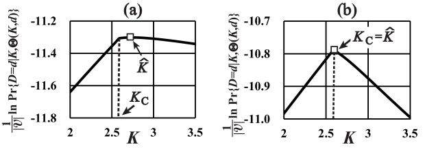
Figure 8: (a) and (b) are the logarithm of marginal likelihood ${\frac{1}{|{\cal{V}}|}}{\ln}{\Pr}{\big{\{}}{\bm{D}}={\bm{d}}{\big{|}}K,{\bm{\Theta}}(K,{\bm{d}}){\big{\}}}$ for the observed images ${\bm{d}}$ in Fig.3(c) and Fig.3(d) in the case of $q=8$, which are shown as black solid curves. $K_{\rm{C}}$ is the first order transition point of the $q$-state Potts model in the loopy belief propagation and is $2.5871$ for $q=8$, respectively.

Figure 9: (a) and (b) are ${\frac{1}{|{\cal{E}}|}}{\displaystyle{{\sum_{\{i,j\}{\in}{\cal{E}}}}}}{\displaystyle{{\sum_{{\bm{a}}}}}}(1-{\delta}_{a_{i},a_{j}}){\Pr}{\big{\{}}{\bm{A}}={\bm{a}}{\big{|}}{\bm{D}}={\bm{d}},K,{\bm{\Theta}}(K,{\bm{d}}){\big{\}}}$ for the observed images ${\bm{d}}$ in Fig.3(c) and Fig.3(d) in the case of $q=8$, which are shown as black solid curves. The red solid curves are $({\alpha}(u),u)$ by using the loopy belief propagation in eqs.(2) and (3). $K_{\rm{C}}$ is the first order transition point of the $q$-state Potts model in the loopy belief propagation and is $2.5871$ for $q=8$, respectively.

5 Concluding Remarks

In the present paper, we proposed a Bayesian image segmentation model based on Potts prior. Under the segmentation model, we then proposed a hyperparameter estimation scheme based on conditional maximization for entropy of the prior, and gave the practical inference algorithm based on LBP.

The conventional maximum likelihood framework, which is based on the maximization of marginal likelihood, is constructed from the free energies of the prior and the posterior probabilities. In the present paper, the prior probability is assumed to be the Potts model and it has the first order phase transition on computing some statistical quantities by means of the LBP. Because the derivative of free energy has discontinuity in the first order phase transition point, it is very difficult to search the maximum point via the extremum condition of the marginal likelihood with respect to some of the hyperparameters. Actually, ${\ln}{\Pr}\{{\bm{D}}={\bm{d}}|u,{\cal{G}}\}$ is given in terms of the normalization constants ${\cal{Y}}({\bm{d}},K,{\bm{\Theta}})$ and ${\cal{Y}}(K)$ in eqs.(55) and (56) as follows:

$${\ln}{\big{(}}{\Pr}\{{\bm{D}}={\bm{d}}|K,{\bm{\Theta}}\}{\big{)}}={\ln}{\big{(}}{\cal{Y}}({\bm{d}},K,{\bm{\Theta}}){\big{)}}-{\ln}{\big{(}}{\cal{Y}}(K){\big{)}}.$$ (66)

The logarithms $-{\ln}{\cal{Y}}(K)$ and $-{\ln}{\cal{Y}}({\bm{d}},K,{\bm{\Theta}})$ correspond to the free energies of the posterior and the prior probabilistic models in eqs.(55) and (56), respectively. As shown in Fig.1, the LBP of the $q$-state Potts prior (55) for $q{\geq}3$ with no external fields have the first order phase transition. In addition, the free energy $f(K)=-{\frac{1}{|{\cal{V}}|}}{\ln}{\cal{Y}}(K)$ per pixel has at least one singular point $K=K_{\rm{C}}$ at which the derivative ${\frac{d}{dK}}f(K)$ is discontinuous with respect to $K$. Although one of the useful procedures for realizing the maximization of marginal likelihood is the EM algorithm[12], it is based on the analysis for hyperparameters and is hard to be adopted in the conventional maximum likelihood framework.

Our proposed algorithm in §3 is based on the constrained maximization of the entropies in eqs.(1) and (22) without using the maximization of marginal likelihood ${\Pr}{\big{\{}}{\bm{D}}={\bm{d}}{\big{|}}K,{\bm{\Theta}}{\big{\}}}$ in eqs.(58) and (66). Particularly, with the $q$-state Potts model in eqs.(2) and (3), the interaction parameter ${\alpha}(u)$ of the $q$-state Potts model (2) is a one-valued function of $u$ which corresponds to the internal energy $-{\frac{1}{2}}{\displaystyle{{\sum_{\{i,j\}{\in}{\cal{E}}}}}}{\displaystyle{{\sum_{\bm{z}}}}}{\delta}_{z_{i},z_{j}}{\Pr}\{{\bm{A}}={\bm{z}}|u\}$, when ${\alpha}(u)$ is regarded as the inverse temperature of the system. It is the key to the success of our iterative inference algorithm (in §3) on estimating the average vectors ${\bm{m}}({\xi})$, covariance matrices ${\bm{C}}({\xi})$ (${\xi}{\in}{\cal{Q}}$), $u$, and ${\alpha}(u)$ in eqs.(19)-(20), as shown in Figs.4 and 5 and Table 1.

In §4, we have conducted the maximization of marginal likelihood ${\Pr}{\big{\{}}{\bm{D}}={\bm{d}}{\big{|}}K,{\bm{\Theta}}{\big{\}}}$ in eqs.(58) and (66) and compare it with our proposed algorithm. The extremum conditions for average vectors ${\bm{m}}({\xi})$ and covariance matrices ${\bm{C}}({\xi})$ (${\xi}{\in}{\cal{Q}}$) have been given by eqs. (61) and (62). They are basically equivalent to the constraints (31) and (32) in our constrained maximization of entropies in eqs.(1) and (22) in §2 and §3. However, their difference is in eq.(59). As mentioned above, ${\Pr}{\big{\{}}{\bm{D}}={\bm{d}}{\big{|}}K,{\bm{\Theta}}{\big{\}}}$ is not differentiable at $K=K_{\rm{C}}$, and therefore the extremum condition of ${\Pr}{\big{\{}}{\bm{D}}={\bm{d}}{\big{|}}K,{\bm{\Theta}}{\big{\}}}$ with respect to $K$ cannot be considered as its maximization when ${\widehat{K}}({\bm{d}})$ is equal to $K_{\rm{C}}$. On the other hand, if ${\widehat{K}}({\bm{d}})$ is equal to $K_{\rm{C}}$, we can consider the extremum condition of ${\Pr}{\big{\{}}{\bm{D}}={\bm{d}}{\big{|}}K,{\bm{\Theta}}{\big{\}}}$ and reduce the deterministic equation of ${\widehat{K}}({\bm{d}})$ to eq.(65). Equation (65) is equivalent to eq.(30). In this case, the conventional maximum likelihood framework in §4 is equivalent to the constrained maximum entropy framework in §2 and §3. The segmentation result for Fig.3(c) in the case of $q=8$ is one of the typical examples, where we obtain ${\alpha}{\big{(}}{\widehat{u}}({\bm{d}}){\big{)}}={\widehat{K}}({\bm{d}})>K_{\rm{C}}$; and the estimates ${\bm{\widehat{\Theta}}}({\bm{d}})$ by using our proposed algorithm are equal to each other, as shown in Table 1.

However, in order to know if ${\widehat{K}}({\bm{d}})$ is equal to $K_{\rm{C}}$ in the conventional maximum likelihood framework, we have to compute ${\Pr}{\big{\{}}{\bm{D}}={\bm{d}}{\big{|}}K,{\bm{\Theta}}(K,{\bm{d}}){\big{\}}}$ to satisfy the simultaneous fixed point equations (61) and (62) with respect to ${\bm{\Theta}}(K,{\bm{d}})$ for various values of $K$, as shown in Fig.8(b). This is the main difficulty for achieving the conventional maximization of marginal likelihood ${\Pr}{\big{\{}}{\bm{D}}={\bm{d}}{\big{|}}K,{\bm{\Theta}}{\big{\}}}$ in eqs.(58) and (66), although our proposed algorithm is constructed from just iterative procedures with respect to ${\widehat{u}}({\bm{d}})$, ${\alpha}{\big{(}}{\widehat{u}}({\bm{d}}){\big{)}}$ and ${\bm{\widehat{\Theta}}}({\bm{d}})$, as shown in “Inference Algorithm for ${\widehat{u}}({\bm{d}})$, ${\alpha}{\big{(}}{\widehat{u}}({\bm{d}}){\big{)}}$ and ${\widehat{\bm{\Theta}}}({\bm{d}})$” of §3.

Finally, we discuss the relationship between the proposed framework and the graph cut method. One may consider using a graph cut method to achieve the image segmentations by means of the MRF. The graph cut methods can derive the exact global maximum configuration ${\bm{a}}^{\bm{*}}$ of the posterior probabilistic distribution ${\Pr}\{{\bm{A}}={\bm{z}}|{\bm{D}}={\bm{d}},K,{\bm{\Theta}}\}$:

$${\bm{a}}^{\bm{*}}={\arg}{\max_{{\bm{z}}}}{\Pr}\{{\bm{A}}={\bm{z}}|{\bm{D}}={\bm{d}},K,{\bm{\Theta}}\},$$ (67)

at least for $q=2$[34], and recently it has been extended to an approximate graph cut method which can be applied also to the case of $q{\geq}3$[35]. However, the graph cut method cannot give the estimates of hyperparameters $K$ and ${\bm{\Theta}}$ from one single observed image ${\bm{d}}$. Instead, the hyperparameter $K$ of the Potts prior is usually estimated by using supervised learning from many labeled pairs $({\bm{a}}^{(1)},{\bm{d}}^{(1)}),({\bm{a}}^{(2)},{\bm{d}}^{(2)}),{\cdots},({\bm{a}}^{(N)},{\bm{d}}^{(N)})$, where the labeled image ${\bm{a}}^{(n)}$ is the ground truth for each observed image ${\bm{d}}^{(n)}$ for $n=1,2,{\cdots},N$. When the supervised learning approaches are included in the graph cut method for image segmentation, the following maximum likelihood estimation is often used for hyperparameter estimation:

$$(K^{*},{\bm{\Theta}}^{\bm{*}})={\arg}{\max_{(K,{\bm{\Theta}})}}{\sum_{n=1}^{N}}{\ln}{\big{(}}{\Pr}\{{\bm{A}}={\bm{a}}^{(n)},{\bm{D}}={\bm{d}}^{(n)}|K,{\bm{\Theta}}\}{\big{)}}.$$ (68)

To sum up, we have clarified the theoretical relationship between the LBP and the graph cut method and have proposed novel statistical methods for probabilistic image segmentations by means of the MRF.

References

References

[1]
H. Derin, H. Elliott, R. Cristi and D. Geman:
IEEE Transactions
on Pattern Analysis and Machine Intelligence,
6 (1984) 707.
[2]
D. Geman:
Lecture Notes in Mathematics,
1427, 113 (Springer-Verlag, Belrin Heidelberg, 1990).
[3]
H. Nishimori: Statistical Physics
of Spin Glass and Information Processing
—Introduction—
(Oxford University Press, Oxford, UK, 2001)
[4]
W. T. Freeman, T. R. Jones and E. C. Pasztor:
IEEE Computer Graphics and Applications,
22 (2002) 56.
[5]
A. S. Willsky:
Proceedings of IEEE, 90 (2002) 1396.
[6]
K. Tanaka:
J. Phys. A: Math. Theor.,
35 (2002) R81.
[7]
Y. Kabashima and D. Saad:
Europhysics Letters, 44 (1998) 668.
[8]
M. Opper and D. Saad (eds):
Advanced Mean Field Methods
— Theory and Practice —
(MIT Press, Cambridge, USA, 2001).
[9]
J. S. Yedidia, W. T. Freeman and Y. Weiss:
IEEE Transaction on Information Theory,
51 (2005) 2282.
[10] A. Pelizzola:
J. Phys. A: Math. Gen.
38 (2005) R309 (Topical Review).
[11]
M. Mézard and A. Montanari:
Information, Physics and Computation
(Oxford University Press, New York, USA, 2009)
[12]
A. P. Dempster, N. M. Laird, D. B. Rubin
and J. Royal:
Statist. Soc. Ser.B, 39 (1977) 1.
[13]
K. Tanaka and D. M. Titterington:
J. Phys. A: Math. Theor.
40 (2007) 11285.
[14]
S. Kataoka and M. Yasuda, K. Tanaka and D. M. Titterington:
Philosophical Magazine, 92 (2012) 50
[15]
Z. Kato and J. Zerubia:
Markov Random Fields in Image Segmentation,
Foundations and Trends in Signal Processing,
Volume 5, Issues 1-2, pp.1-155
(now Publishers Inc., Hanover, USA).
[16]
S. Lakshmanan and H. Derin:
IEEE Transactions on Pattern Analysis
and Machine Intelligence, 11 (1989) 799.
[17]
J. Zhang:
IEEE Trans. Image Processing, 40 (1994) 2570.
[18]
J. Zhang, J. W. Modestino and D. A. Langan:
IEEE Transactions on Image processing, 3 (1994) 404.
[19]
C. D’Elia, G. Poggi and G. Scarpa:
IEEE Transactions on Image Processing, 12 (2003) 1259.
[20]
L. Cheng, F. Jiao, D. Schuurmans, S. Wang:
Proceedings of the 22nd International Conference
on Machine Learning (Association for Computing Machinery,
New York, USA, 2005) 129.
[21]
F. Chen, K. Tanaka and T. Horiguchi:
Interdisciplinary Information Sciences, 11 (2005) 17.
[22]
C. A. McGrory, D. M. Titterington, R. Reeves and A. N. Pettitt:
Statistics and Computing, 19 (2009) 329.
[23]
S. Miyoshi and M. Okada:
J. Phys. Soc. Jpn, 80 (2011) 014802.
[24]
R. Hasegawa, M. Okada and S. Miyoshi:
J. Phys. Soc. Jpn, 80 (2011) 093802.
[25]
J. Gimenez, A. C. Frery and A. G. Flesia:
IEEE International Geoscience and Remote Sensing Symposium
(Melbourne, Australia, 2013)
[26]
D. M. Carlucci and J. Inoue:
Phys. Rev. E, 60 (1999) 2547.
[27]
H. Nishimori and G. Ortiz:
Elements of Phase Transitions
and Critical Phenomena
(Oxford University Press, Oxford, UK, 2010)
[28]
K. Tanaka, S. Kataoka and M. Yasuda:
Journal of Physics: Conference Series,
233 (2010) 012013.
[29]
K. Tanaka and D. M. Titterington:
Progress of Theoretical Physics,
Supplement, 157 (2005) 288.
[30]
K. Tanaka, M. Yasuda and D. M. Titterington:
J. Phys. Soc. Jpn, 81 (2012) 114802.
[31] The images in Fig.3(a)-(c)
are in the Berkeley Segmentation Data Set 500 (BSDS500),
which is available at
http://www.eecs.berkeley.edu/Research/Projects/CS/vision/grouping/.
[32]
P. Arbelaez, M. Maire, C. Fowlkes and J. Malik:
IEEE Transactions
on Pattern Analysis and Machine Intelligence,
33 (2011) 898.
[33] The images in Fig.3(d)-(f)
are in the USC-SIPI (Signal and Image Processing Institute,
University of Southern California) Image Database,
which is available at
http://sipi.usc.edu/database/.
[34]
Y. Boykov, O. Veksler and R. Zabih:
IEEE Transactions
on Pattern Analysis and Machine Intelligence,
23 (2001) 1222.
[35]
K. Alahari, P. Kohli and P. H. S. Torr:
IEEE Transactions
on Pattern Analysis and Machine Intelligence,
32 (2010) 1846.