Variational Approach to Localization Length for Two-Dimensional Hubbard Model

Abstract

As a measure to ascertain whether a system is metallic or insulating, localization length $\lambda_{N}$, which represents the spread of electron distribution, can be a useful quantity, especially for approaching a metal-insulator transition from the insulator side. We try to calculate $\lambda_{N}$ using a variational Monte Carlo method for normal (paramagnetic), superconducting and antiferromagnetic states in the square-lattice Hubbard model. It is found that the behavior of $\lambda_{N}$ is consistent with what is expected from other quantities, and gives information complementary to another measure, the Drude weight.

1 Introduction

Because, in many strongly correlated electron systems, itinerancy and localization of conduction electrons are vital to their properties, appropriate and convenient measures to determine whether the system is a metal or an insulator have been pursued for long years. Various physical quantities are available to consider metal-insulator transitions, such as quasi-particle renormalization factor $Z$, charge structure factor $N({\bf q})$, chemical potential $\mu$ and the Drude weight $D$, DC component of conductivity, introduced by Kohn[1, 2]. Because these quantities are obtained within ground states, the nature of being a metal or an insulator is already inherent in the ground-state wave functions. Correctly, $N({\bf q})$ and $\mu$ are not measures, and the vanishing of $Z$ do not necessarily indicate an insulator, but represent a gap opening in some degree of freedom. Actually, $Z$ do not distinguish an $s$-wave superconducting (SC) state (gapped in the spin sector, but gapless in the charge sector) from an insulating state (gapped in the charge sector). As for $\mu$ [3], we have to find a jump as a function of electron density $n$ ($=N/N_{\rm s}$; $N$: electron number, $N_{\rm s}$: site number) or doping rate $\delta$ ($=1-n$), in addition to differentiating the total energy with respect to $n$. It is a little laborious. Here, we are interested in strongly correlated systems, for which a variational Monte Carlo (VMC) method[4] is very useful for its exact treatment of local electron correlation without a minus sign problem. Thus, in this work, we discuss useful measures of metal-insulator transitions for VMC calculations, namely, $D$ and in particular localzation length $\lambda_{N}$. We adopt a Hubbard model on the square lattice, which is a plausible model of the cuprate superconductors, and undergoes a Mott transition at half filling at $U\sim W$ (band width), unless an antiferromagnetic (AF) order is assumed.

Since the discovery of cuprate superconductors, $D$ has been intensively studied, because $D$ is directly obtained from experiments; in particular, anomalous $\delta$ dependence of superfluid density $\rho_{\rm s}$[5], which is equivalent to $D$ in SC states[2], in cuprates is regarded as indubitable evidence of a doped Mott insulator. To obtain $D$ in the two-dimensional Hubbard model, we have to calculate the ground-state energy of the Hamiltonian[6],

$${\cal H}(\mathbb{A})=-t\sum_{<i,j>,\>\sigma}\left[e^{i\mathbb{A}\cdot(\mathbb{r}_{i}-\mathbb{r}_{j})}c_{i\sigma}^{\dagger}c_{j\sigma}+\mathrm{H.c.}\right]+U\sum_{j}n_{j\uparrow}n_{j\downarrow},$$ (1)

where $c_{j\sigma}(c_{j\sigma}^{\dagger})$ is the electron annihiration (creation) operator of spin $\sigma$ at site $j$, $n_{j\sigma}=c_{j\sigma}^{\dagger}c_{j\sigma}$, $t$ (hopping integral) and $U$ (onsite interaction) are positive variables, and $\mathbb{A}$ is a virtual vector potential. $D$ is given by $D=d^{2}E(A)/dA^{2}$ with $E(A)=\langle{\cal H}(\mathbb{A})\rangle$. If the system is metallic (insulating), $D$ is finite (vanishes). In variation theories, however, a metal-insulator transition had not been described by means of $D$ until recently[7], namely, $D$ remained positive finite in insulating states even if binding factors between a doubly occupied site (doublon) and an empty site (holon)[8] are introduced, with which Mott transitions are definitely described in terms of other quantities. Recently, this problem was solved as far as the range of $U\gtrsim U_{\rm c}$ ($U_{\rm c}/t$: Mott transition point) is concerned[6]. The ground state of eq. (1) must be essentially complex, because the matrix elements are complex owing to the Peierls phase $e^{i\mathbb{A}\cdot(\mathbb{r}_{i}-\mathbb{r}_{j})}$. Therefore, an appropriate wave function should have a configuration-dependent phase factor ${\cal P}_{\theta}$[6]. Thereby, not only Mott transitions are clearly identified by $D$, but linear behavior of $\rho_{\rm s}(\delta)$ (Uemura plot)[5] is obtained. We now know that this type of phase factors are indispensable for addressing current-carrying states such as various flux states[9] for intermediate and strong correlations. On the other hand, for insulators in weakly correlated regimes such as Slater-type AF insulators, we found that appropriate trial wave functions for finite A should consist of multiple determinants; it seems technically difficult to treat them with the present VMC scheme[6]. In calculating $D$, fine tuning of the trial functions seems necessary according to individual cases.

Although $D$ gives useful information in a metallic regime, $D$ does not tell how rigidly electrons are bound in an insulating regime, where $D$ always vanishes. As an alternative measure of metal-insulator transition from the insulator side, Resta[10, 11] introduced localization length $\lambda_{N}$, which approaches the spread of the electronic distribution, $\sqrt{[\langle(\sum_{j}x_{j})^{2}\rangle-\langle\sum_{j}x_{j}\rangle^{2}]/N}$, as the system size increases. $\lambda_{N}$ represents how electrons can broaden in an insulating state; we can judge that the system is insulating (metallic), if $\lambda_{N}$ remains finite (diverges) as the system size is increased to infinity. Thus, a Mott transition point can be determined by the diverging point of $\lambda_{N}$, without carrying out differentiating operations in contrast to $D$. In early studies for one-dimensional systems, $\lambda_{N}$ or a corresponding susceptibility was calculated using exact diagonalization[11], quantum Monte Carlo method[12], and density matrix renormalization group[13]. Regarding VMC, $\lambda_{N}$ was calculated for a hydrogen chain[14]; it seems that $\lambda_{N}$ can be a good measure.

In the following, we calculate the localization length in a Hubbard model on the square lattice [eq. (1) with ${\bf A}={\bf 0}$] using a VMC method, to confirm that $\lambda_{N}$ is an appropriate measure of a Mott transition. In sec. 2, we describe the method used in this study. In sec. 3, we show results of $\lambda_{N}$, and have discussions. A conclusion is given in sec. 4.

2 Method

In this section, we briefly explain variational wave functions used and the localization length $\lambda_{N}$. We study $\lambda_{N}$ with three types of wave functions: (i) a $d_{x^{2}-y^{2}}$-wave superconducting (SC) or singlet-pairing state $\Psi_{\mathrm{SC}}$, (ii) a paramagnetic or normal state $\Psi_{\mathrm{N}}$, and (iii) an AF state $\Psi_{\mathrm{AF}}$. Because these functions are applied to a highly correlated Hamiltonian, we adopt short-range Jastrow-type wave functions, which are composed of two parts: $\Psi={\cal P}\Phi$. Here, $\Phi$ represents a one-body wave function, $\Phi=\Phi_{\mathrm{SC}}$, $\Phi_{\mathrm{N}}$ or $\Phi_{\mathrm{AF}}$, each of which is a solution of the Hartree-Fock approximation without imposing the SCF condition. They are explicitly written as,

$$\Phi_{\mathrm{SC}} = \left(\sum_{\mathbb{k}}a_{\mathbb{k}}c_{\mathbb{k}\uparrow}^{\dagger}c_{-\mathbb{k}\downarrow}^{\dagger}\right)^{N/2}|0\rangle,\qquad a_{\mathbb{k}}=\frac{\Delta_{d}(\mathbb{k})}{\varepsilon_{\mathbb{k}}-\zeta+\sqrt{(\varepsilon_{\mathbb{k}}-\zeta)^{2}+|\Delta_{d}(\mathbb{k})|^{2}}},$$ (2)

$$\Phi_{\mathrm{N}} = \prod_{k\in\mathrm{FS},\ \sigma}c_{k\sigma}^{\dagger}|0\rangle,\qquad\qquad\mbox{(FS: Fermi sea)}$$ (3)

$$\Phi_{\mathrm{AF}} = \prod_{\mathbb{k},\sigma}\left(\alpha_{\mathbb{k}}c_{\mathbb{k}\sigma}^{\dagger}+\tilde{\sigma}\beta_{\bf k}c_{\mathbb{k+Q}\sigma}^{\dagger}\right)|0\rangle,\qquad\alpha_{\mathbb{k}}\left(\beta_{\mathbb{k}}\right)=\sqrt{\frac{1}{2}\left(1-(+)\frac{\varepsilon_{\mathbb{k}}}{\sqrt{\varepsilon_{\mathbb{k}}^{2}+\Delta_{\mathrm{AF}}^{2}}}\right)}.$$ (4)

In $d$-wave BCS wave function $\Phi_{\mathrm{SC}}$, $\varepsilon_{\mathbb{k}}=-2t(\cos k_{x}+\cos k_{y})$, $\zeta$ is a variational parameter corresponding to the chemical potential in the limit of $U/t\rightarrow 0$, and the pair potential is assumed as $\Delta_{d}(\mathbb{k})=\Delta(\cos k_{x}-\cos k_{y})$ with $\Delta$ being a variational parameter. In $\Phi_{\mathrm{AF}}$, $\tilde{\sigma}=\pm 1$ according to $\sigma=\uparrow$ or $\downarrow$, $\mathbb{Q}=(\pi,\pi)$, and $\Delta_{\mathrm{AF}}$ is a variational parameter related to the staggered moment. As for the many-body part ${\cal P}$ in $\Psi$, we consider only dominant factors, ${\cal P}={\cal P}_{\mathrm{G}}{\cal P}_{Q}$, in common for the three $\Psi$’s. The most fundamental one is the onsite (Gutzwiller) factor, ${\cal P}_{\mathrm{G}}=\prod_{j}[1-(1-g)n_{j\uparrow}n_{j\downarrow}]$ with $g$ being a variational parameter ($0\leq g\leq 1$). The second factor is a doublon-holon binding factor between nearest-neighbor (NN) sites [8], which is indispensable for inducing a Mott transition: ${\cal P}_{Q}=\prod_{j}[1-\mu_{1}Q_{j}^{1}]\prod_{i}[1-\mu_{2}Q_{i}^{2}]$, with $Q_{j}^{1}=n_{j\uparrow}n_{j\downarrow}\prod_{\tau}[1-(1-n_{j+\tau\uparrow})(1-n_{j+\tau\downarrow})]$, and $Q_{j}^{2}=(1-n_{j\uparrow})(1-n_{j\downarrow})\prod_{\tau}(1-n_{j+\tau\uparrow}n_{j+\tau\downarrow})$. Here, $\mu_{1}$ and $\mu_{2}$ are variational parameters ($0\leq\mu_{1},\>\mu_{2}\leq 1$), and $\tau$ runs over the NN sites of site $j$. Some properties of these wave functions when applied to eq. (1) are known [15, 16, 17, 6]. At half filling, it was confirmed through the behavior of $Z$, $N({\bf q})$, $D$, etc. that $\Psi_{\mathrm{SC}}$ and $\Psi_{\mathrm{N}}$ exhibit first-order Mott transitions at $U/t\sim 6.5$ and $8.5$, respectively. On the other hand, it is expected that an AF state becomes the ground state and insulating for any $U/t$ $(>0)$ without transitions. Actually, $\Psi_{\mathrm{AF}}$ is insulating and has the lowest energy among the three $\Psi$’s for $U/t\gtrsim 1.5$. For $0<U/t\lesssim 1.5$, the AF order seems to vanish in $\Psi_{\mathrm{AF}}$, but this is irrelevant to the following discussions. In less-than-half-filled cases, the three $\Psi$’s are always metallic.

In an insulator (metal), the ground-state wave function is localized (delocalized). In a system under the periodic boundary condition, localization can be treated in parallel with the modern theory of polarization[10, 11]. The degree of localization is embedded in a complex number $z_{N}$ defined below, whose modulus is the definition of localization length $\lambda_{N}$:

$$\lambda_{N}=\left(\frac{L}{2\pi}\right)\sqrt{-\frac{\ln|z_{N}|^{2}}{N}}\hskip 14.22636pt\mathrm{with}\hskip 14.22636ptz_{N}=\langle\Psi|e^{i\frac{2\pi}{L}X}|\Psi\rangle\qquad(L\rightarrow\infty),$$ (5)

where $L$ is the system size in one ($x$) direction, and $X$ is the sum of $x$ coordinates of electrons: $X=\sum_{j,\sigma}x_{j}n_{j\sigma}$. If we expand $z_{N}$ with respect to $2\pi/L$ and substitute it in the expression of $\lambda_{N}$ in eq. (5), the definition of localization length, $\sqrt{(\langle X^{2}\rangle-\langle X\rangle^{2})/N}$, is obtained as the leading term. Therefore, we should check $L$ dependence of $\lambda_{N}$ to monitor the deviation owing to higher-order terms. When the state is extremely localized like a $\delta$ function, $z_{N}$ becomes 1; $z_{N}$ is finite ($0<|z_{N}|<1$) for general localized states, whereas $z_{N}$ vanishes when the state is delocalized. Equivalently, $\lambda_{N}$ converges to a finite value for an insulator, but diverges as $L$ increases for a metallic system. Using the above wave functions, the expectation value of $z_{N}$ is easily calculated by VMC.

We carry out a series of VMC calculations to estimate $z_{N}$ using correlated measurement with quasi-Newton algorithm for large systems of $L\times L$ sites ($L=12$-$20$). A typical sample number in this study is $M=2.4\times 10^{5}$.

3 Results

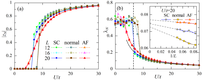
Figure 1: (Color online) (a) Absolute values of $z_{N}$ are shown for the three $\Psi$’s as a function of $U/t$ at half filling for three $L$’s. (b) Localization length are compared among the three wave functions. The symbols are common to (a). A dash-dotted curve of $\propto t/U$ is added as a guide for eyes. The vertical dashed line indicates the metal-insulator transition point of $\Psi_{\rm SC}$. Inset in (b) shows the extrapolation of $\lambda_{N}$ to $L\rightarrow\infty$ for the three states for $U/t=20$ from the data for $L=12$-$20$. The number of samples is $2.4\times 10^{5}$.

Let us start with $U/t$ dependence of $|z_{N}|$ at half filling. In Fig. 1(a), we plot $|z_{N}|$ obtained by VMC calculations for the three states. For $\Psi_{\rm SC}$, $|z_{N}|$ is almost zero for $U/t\leq 6$, but suddenly increases with a jump at approximately $U/t=6.5$, and tends to unity for $U/t\geq 7$. As mentioned above, this behavior of $|z_{N}|$ indicates that the system is conductive (insulating) for $U/t<6.5$ ($U/t>6.5$), and at $U/t=6.5$ a sharp (first-order-like) SC-insulator transition arises. This result is quantitatively consistent with that of the previous studies[15, 16, 6], in which this Mott transition was confirmed by various quantities such as a SC pairing correlation function and the Drude weight. The behavior of $|z_{N}|$ of $\Psi_{\rm N}$ is similar to that of $\Psi_{\rm SC}$ except for the Mott transition point, and is consistent with that of the previous results. Although appreciable system-size dependence in $|z_{N}|$ is observed both for $\Psi_{\rm SC}$ and $\Psi_{\rm N}$, especially near the transition points, they will not qualitatively change the features of Mott transition. We will return to this point again in connection with $\lambda_{N}$. $|z_{N}|$ of $\Psi_{\rm AF}$ is again almost zero for $0<U/t\leq 3$, but this time $|z_{N}|$ increases smoothly for $U/t>3$, as $U/t$ increases, without anomalous behavior like a jump. Thus, $\Psi_{\rm AF}$ is insulating at least for $U/t>3$. Considering $\Psi_{\rm AF}$ is insulating for more smaller values of $U/t$, we expect that the value of $|z_{N}|$ is very small but still non zero for $U/t<3$. In this range, it is difficult to determine the accurate behavior of $|z_{N}|$, because statistical errors in VMC exceed the magnitude of $|z_{N}|$. We will discuss this point later again. The system-size dependence for $\Psi_{\rm AF}$ is by far smaller than those for $\Psi_{\rm SC}$ and $\Psi_{\rm N}$.

We turn to the localization length $\lambda_{N}$, which is calculated from $z_{N}$ through eq. (5). In Fig. 1(b), we plot $\lambda_{N}$ obtained from the data in Fig. 1(a). As a whole, $\lambda_{N}$ tends to decrease as $U/t$ increases; this behavior agrees with our intuition that the electrons are more localized as the repulsive interaction becomes stronger. Corresponding to the behavior of $|z_{N}|$, $\lambda_{N}$ for $\Psi_{\rm SC}$ and $\Psi_{\rm N}$ exhibit discontinuities at $U/t=6.5$ and $8.5$, respectively; $\lambda_{N}$ of $\Psi_{\rm AF}$ is smooth for $U/t\gtrsim 3$.

First, we discuss the insulating regimes. Here, each $\lambda_{N}$ decreases approximately as a function of $t/U$ ($=J/4t$), indicating that the insulating regime is effectively described by an AF Heisenberg model with the exchange coupling $\sim J$, which is the sole energy scale. Now, we look at the system-size dependence. In the inset of Fig. 1, we plot $\lambda_{N}$ at $U/t=20$ in the insulating regime as a function of $1/L$. The system-size dependence is the largest in $\Psi_{\rm N}$ and the smallest in $\Psi_{\rm AF}$, but the order among the three does not seem to change in the limit of $L\rightarrow\infty$. The localization length of $\Psi_{\rm SC}$ is a little longer than that of $\Psi_{\rm N}$, indicating electrons in SC is more mobile than in the normal state even in a insulating regime. This corresponds to the fact that the kinetic energy is lower for $\Psi_{\rm SC}$ than for $\Psi_{\rm N}$ (not shown), namely, a kinetic-energy-driven SC ($\Psi_{\rm N}\rightarrow\Psi_{\rm SC}$) transition is realized, as previous studies showed[15]. Incidentally, for smaller values of $U/t$ ($U_{\rm c}<U<20t$), we cannot implement reliable extrapolations for $\Psi_{\rm SC}$ and especially $\Psi_{\rm N}$, because the system-size dependence of $\lambda_{N}$ becomes somewhat irregular. It seems that this is not only owing to the sampling errors but to the short range nature of the trial wave functions. It is possible that a long-range correlation factor is necessary for systems of large $\lambda_{N}$ to stably estimate $\lambda_{N}$ near Mott transitions. The notion of a kinetic-energy-driven transition is similarly applicable to the AF transition ($\Psi_{\rm N}\rightarrow\Psi_{\rm AF}$), because $\lambda_{N}^{\rm AF}>\lambda_{N}^{\rm N}$. The reason $\lambda_{N}^{\rm AF}$ is the largest is that electrons are more likely to hop to NN sites owing to the spin alternate configurations in $\Psi_{\rm AF}$.

Next, we consider the results of $\lambda_{N}$ in weakly correlated regimes. In the insulating regimes discussed above, the expectation values of $\lambda_{N}$ converges at finite values, as expected. On the other hand, in weakly correlated regimes ($U<U_{\rm c}$ for $\Psi_{\rm SC}$ and $\Psi_{\rm N}$; $U\lesssim 3t$ for $\Psi_{\rm AF}$), $\lambda_{N}$ does not diverge as $L\rightarrow\infty$, but has scattered values around 0.6 irrespective of the system size, as found in Fig. 1(b). An origin of this result probably lies in the statistical errors in VMC sampling. The expectation values of $|z_{N}|$ for these correlation strengths are extremely close to zero but positive finite. Therefore, if the numerical error $\epsilon$ exceeds the correct expectation value, the estimation by VMC yields an arbitrary value of order $\epsilon$ as $|z_{N}|$. To verify this possibility, we carry out a series of VMC calculations for $\Psi_{\rm SC}$ by widely varing the sampling number $M$ for a fixed $L$ ($=12$); the statistical errors are proportional to $1/\sqrt{M}$. The results are plotted in Fig. 2(a). We find that the value of $\lambda_{N}$ steadily increases as $M$ increases, although the increments are small because $\lambda_{N}$ is a logarithmic function of $|z_{N}|$ [eq. (5)]. Thus, in order to estimate $\lambda_{N}$ accurately for a system with large $\lambda_{N}$, it is necessary to precisely determine $|z_{N}|$ of a large negative power. In this connection, we calculate $\lambda_{N}$ for less-than-half-filled or doped systems, which are metallic for any value of $U/t$, with the same sample number as in Fig. 1(b). As shown in Fig. 2(b), the results are scattered around $\lambda_{N}=0.6$ in broad accordance with that for the weakly interacted half-filled case in Fig. 1(b). We can perceive a slight tendency for $\lambda_{N}$ to increases as electron density ($n$) decreases. Anyway, the present VMC calculations yield a reliable value of $\lambda_{N}$ for an insulator of $\lambda_{N}\lesssim 0.5$.

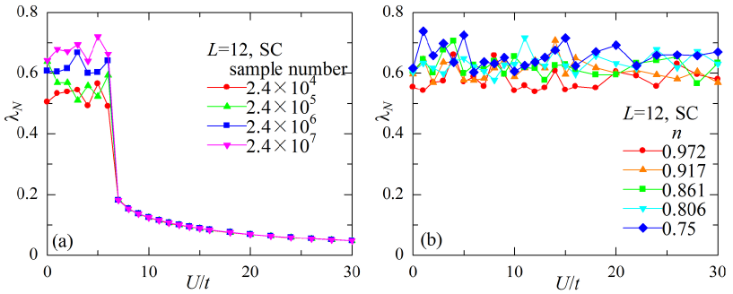
Figure 2: (Color online) (a) Expectation values of localization length at half filling are compared for different sample numbers in the VMC calculations for $\Psi_{\rm SC}$. (b) Localization length estimated with the same VMC procedure for several doped systems. $n$ indicates an electron density. The number of sample is $2.4\times 10^{5}$.

Finally, we touch on $\lambda_{N}$ of $\Psi_{\rm AF}$. Judging from other quantities, $\Psi_{\rm AF}$ is insulating at least for $U/t\gtrsim 1.5$, as mentioned. Therefore, $\lambda_{N}$ should converge at finite values in this range. Correspondingly, $\lambda_{N}$ in Fig. 1(b) exhibits a smooth converged curve for large values of $U/t$ down to $U/t\sim 3$. However, at $U/t=3$, $\lambda_{N}$ reaches 0.6 still in the insulating phase. Thus, to address an insulator in weak-correlation regimes, a formalism or an algorithm in a new line seems necessary.

4 Summary

Localization length $\lambda_{N}$, which is the variance in coordinates of electrons, is calculated for the two-dimensional Hubbard model to distinguish a metal from an insulator, using a variational Monte Carlo method. $\lambda_{N}$ thus obtained definitely indicates a Mott transition point ($U_{\rm c}$) by a discontinuity for a normal or a $d$-wave pairing state, whose $U_{\rm c}$ is at a correlation strength broadly of the band width. On the other hand, we found that reliable estimation of $\lambda_{N}$ by VMC is not easy for a system of $\lambda_{N}$ beyond a threshold value determined by the numerical errors ($\sim 0.6$ in the present setting), regardless of being a metal or an insulator. Therefore, the present scheme is not necessarily suitable to address weakly correlated insulators such as a Slater-type antiferromagnetic insulator. Nevertheless, we may say that $\lambda_{N}$ is a useful quantity to discuss Mott transitions using various Monte Carlo methods.

References

- [1] W. Kohn: Phys. Rev. 133 (1964) A171.
- [2] D. J. Scalapino, S. R. White, and S. Zhang: Phys. Rev. B 47 (1993) 7995.
- [3] N. Furukawa and M. Imada: J. Phys. Soc. Jpn. 62 (1993) 2557.
- [4] W. L. McMillan: Phys. Rev. 138 (1965) A442; D. Ceperley, G. V. Chester, and M. H. Kalos: Phys. Rev. B 16 (1977) 3081.
- [5] Y. J. Uemura: J. Phys. Cond. Mat. 16 (2004) S4515; C. Bernhand, J .L. Tallon, Th. Blasius, A. Golnik, and Ch. Niedermayer: Phys. Rev. Lett. 86 (2001) 1614.
- [6] S. Tamura and H. Yokoyama: Phys. Proc. 45 (2013) 5, and in preparation.
- [7] A. J. Millis and S. N. Coppersmith: Phys. Rev. B 43 (1991) 13770.
- [8] H. Yokoyama, and H. Shiba: J. Phys. Soc. Jpn. 59 (1990) 3669.
- [9] H. Yokoyama, S. Tamura, and M. Ogata: submitted to J. Phys. Soc. Jpn., and in preparation.
- [10] R. Resta: Phys. Rev. Lett. 80 (1998) 1800.
- [11] R. Resta and S. Sorella: Phys. Rev. Lett. 82 (1999) 370.
- [12] T. Wilkens and R. M. Martin: Phys. Rev. B 63 (2001) 235108.
- [13] C. Aebischer, D. Baeriswyl, and R. M. Noack: Phys. Rev. Lett. 86 (2001) 468.
- [14] L. Stella, C. Attaccalite, S. Sorella, and A. Rubio: Phys. Rev. B 84 (2011) 245117.
- [15] H. Yokoyama, Y. Tanaka, M. Ogata, and H. Tsuchiura: J. Phys. Soc. Jpn. 73 (2004) 1119.
- [16] H. Yokoyama, M. Ogata, and Y. Tanaka: J. Phys. Soc. Jpn. 75 (2006) 114706.
- [17] H. Yokoyama, M. Ogata, Y. Tanaka, K. Kobayashi, and H. Tsuchiura: J. Phys. Soc. Jpn. 82 (2013) 014707.