Effects of discontinuities of the derivatives of the inflaton potential

Alexander Gallego Cadavid3,2, Antonio Enea Romano3,1,2 1Department of Physics, University of Crete, 71003 Heraklion,Greece
2Yukawa Institute for Theoretical Physics, Kyoto University, Japan
3Instituto de Fisica, Universidad de Antioquia, A.A.1226, Medellin, Colombia
Abstract

We study the effects of a class of features of the inflaton potential, corresponding to discontinuties in its derivatives. We perform fully numerical calculations and derive analytical approximations for the curvature pertubations spectrum and the bispectrum which are in good agreement with the numerical results.

The spectrum of primordial perturbations has oscillations around the scale k0subscript𝑘0k_{0} which leaves the horizon at the time τ0subscript𝜏0\tau_{0} when the feature occurs, with the amplitude and phase of the oscillations determined by the size and the order of the discontinuity. The large scale bispectrum in the squeezed and equilateral limits have a very similar form and are linearly suppressed. Both in the squeezed and equilateral small scale limit the bispectrum has an oscillatory behavior whose phase depends on the parameters determining the discontinuity, and whose amplitude is inversely proportional to the scale. Given the generality of this class of features they could be used to model or classify phenomenologically different types of non Gaussian features encountered in observational data such as the cosmic microwave background radiation or large scale structure.

I Introduction

In the last few decades the outstanding advances in observational cosmology have allowed for the first time to test theoretical cosmological models et ; wmapcpr ; pxvi ; inflation2014 . Among the most important sources of cosmological observational data we can mention the Sloan Digital Sky Survey (SDSS), the Wilkinson Microwave Anisotropy Probe (WMAP), and the Planck mission, and other ground-based and sub-orbital experiments gbe1 ; gbe2 . According to the standard cosmological model the cosmic microwave background (CMB) radiation consists of photons which decoupled from the primordial plasma at the time when protons and electrons combined to form neutral light atoms. Although this radiation is extremely isotropic there are small fluctuations in the temperature of the order of ΔT/T105similar-toΔ𝑇𝑇superscript105\Delta T/T\sim 10^{-5}. And since the CMB radiation was emitted at a redshift of about 110011001100 it provides a unique window on the early universe wmapfmr ; pxxii ; xc .

Inflation theory anewtype explains the anisotropies of the CMB temperature as the consequence of primordial curvature perturbations whose statistical properties can be described by the n-points correlation functions. If the perturbations followed a perfectly Gaussian distribution the two points correlation function would be enough, but even the most recent observations are compatible with some non Gaussianity corresponding to fNLlocal=2.5±5.7superscriptsubscript𝑓𝑁𝐿𝑙𝑜𝑐𝑎𝑙plus-or-minus2.55.7f_{NL}^{local}=2.5\pm 5.7 and fNLequil=16±70superscriptsubscript𝑓𝑁𝐿𝑒𝑞𝑢𝑖𝑙plus-or-minus1670f_{NL}^{equil}=-16\pm 70 pxxii ; pxxiv , motivating the theoretical study of the conditions which could have generated it. Some recent developments in the study of models which could generate non Gaussianity and on their detection can be found for example in Hazra:2012yn ; Dorn:2014kga ; bingo ; numerical2013 .

The theoretical study of the effects of features of the inflaton potential was started in the seminal works of Starobinsky starobinsky , and once CMB observational data became available it was shown that features can be used to model the glitches of the power spectrum constraints1 ; constraints2 . Some other interesting studies and reviews in this area can be found for example in Starobinsky:1998mj ; Joy:2007na ; Joy:2008qd ; Mortonson:2009qv . In this paper we focus on the effects of features of the inflaton potential on the primordial curvature perturbations, considering a class corresponding to a discontinuity in the derivatives of the potential. Our model is a generalization of other features which have been studied earlier such as the Starobinsky model or the mass step aer . These kinds of features could have arisen through different mechanisms such as for example particle production pp , or phase transitions Adams2 , but in this paper we study their effects from a purely phenomenological point of view, without investigating their fundamental origin.

There is also an important observational motivation for studying this kind of potentials: recent analyses of CMB observations based on cubic Hermite interpolating polynomials (PCHIP) for the primordial curvature perturbations spectrum Gariazzo:2014dla have in fact shown some evidence for a feature around the wave number k=0.002𝑘0.002k=0.002 Mpc-1, which is in good qualitative agreement with the results of our calculations for some of the potentials we consider.

The paper is organized as following: first we define the features, then we give both a numerical and analytical solution for the background, and finally provide both numerical and analytical calculations of the spectrum and the bispectrum, giving details of the squeeze and equilateral limit and show the effects of varying the different parameters defining the feature, i.e., its amplitude and the order n𝑛n of the discontinuous derivatives.

II Inflation

We consider inflationary models with a single scalar field and a standard kinetic term according to the action linf ; inf

S=d4xg[12MPl2R12gμνμϕνϕV(ϕ)],𝑆superscript𝑑4𝑥𝑔delimited-[]12subscriptsuperscript𝑀2𝑃𝑙𝑅12superscript𝑔𝜇𝜈subscript𝜇italic-ϕsubscript𝜈italic-ϕ𝑉italic-ϕS=\int d^{4}x\sqrt{-g}\left[\frac{1}{2}M^{2}_{Pl}R-\frac{1}{2}g^{\mu\nu}\partial_{\mu}\phi\partial_{\nu}\phi-V(\phi)\right], (1)

where MPl=(8πG)1/2subscript𝑀𝑃𝑙superscript8𝜋𝐺12M_{Pl}=(8\pi G)^{-1/2} is the reduced Planck mass. Varying the action with respect to the metric tensor and the scalar field we get Friedmann equation and the equation of motion of the inflaton

H2(a˙a)2=13MPl2(12ϕ˙2+V(ϕ)),superscript𝐻2superscript˙𝑎𝑎213subscriptsuperscript𝑀2𝑃𝑙12superscript˙italic-ϕ2𝑉italic-ϕH^{2}\equiv\left(\frac{\dot{a}}{a}\right)^{2}=\frac{1}{3M^{2}_{Pl}}\left(\frac{1}{2}\dot{\phi}^{2}+V(\phi)\right), (2)
ϕ¨+3Hϕ˙+ϕV=0,¨italic-ϕ3𝐻˙italic-ϕsubscriptitalic-ϕ𝑉0\ddot{\phi}+3H\dot{\phi}+\partial_{\phi}V=0, (3)

where dots and ϕsubscriptitalic-ϕ\partial_{\phi} indicate derivatives with respect to time and scalar field respectively and H𝐻H is the Hubble parameter. We adopt the following definitions of the slow roll parameters

ϵH˙H2,ηϵ˙ϵH.formulae-sequenceitalic-ϵ˙𝐻superscript𝐻2𝜂˙italic-ϵitalic-ϵ𝐻\displaystyle\epsilon\equiv-\frac{\dot{H}}{H^{2}}\,\,\,\,,\,\,\,\,\eta\equiv\frac{\dot{\epsilon}}{\epsilon H}. (4)

III The model

We consider a single scalar field ϕitalic-ϕ\phi with potential

V(ϕ)={Vb+12m2ϕ2,ϕ>ϕ0Va+12m2ϕ2+λΔϕ,ϕ<ϕ0𝑉italic-ϕcasessubscript𝑉𝑏12superscript𝑚2superscriptitalic-ϕ2italic-ϕsubscriptitalic-ϕ0subscript𝑉𝑎12superscript𝑚2superscriptitalic-ϕ2𝜆Δitalic-ϕitalic-ϕsubscriptitalic-ϕ0V(\phi)=\left\{\begin{array}[]{lr}V_{b}+\frac{1}{2}m^{2}\phi^{2},&\phi>\phi_{0}\\ V_{a}+\frac{1}{2}m^{2}\phi^{2}+\lambda\Delta\phi,&\phi<\phi_{0}\end{array}\right. (5)

where

Δϕϕn.Δitalic-ϕsuperscriptitalic-ϕ𝑛\displaystyle\Delta\phi\equiv\phi^{n}. (6)

where Vasubscript𝑉𝑎V_{a} and Vbsubscript𝑉𝑏V_{b} are different in order to ensure the continuity of the potential at ϕ0subscriptitalic-ϕ0\phi_{0}.

The value of ϕ0subscriptitalic-ϕ0\phi_{0} determines the scale at which the effects of the feature appear in the power spectrum and the bispectrum of curvature perturbations, and as such it is a free parameter which can be fixed phenomenologically based on experimental data. It is in fact determining the value of conformal time when ϕ(τ0)=ϕ0italic-ϕsubscript𝜏0subscriptitalic-ϕ0\phi(\tau_{0})=\phi_{0}, and as it will be shown in the following sections the features in the spectrum and bispectrum appear around the scale k0=1/τ0subscript𝑘01subscript𝜏0k_{0}=-1/\tau_{0} which is leaving the horizon at that time.

The potential has a discontinuity in the derivatives at ϕ0subscriptitalic-ϕ0\phi_{0}, which is the cause of the temporary slow roll regime violation which produce the non Gaussian features. The continuity condition for the potential at τ0subscript𝜏0\tau_{0} gives

Va=Vbλϕ0n.subscript𝑉𝑎subscript𝑉𝑏𝜆superscriptsubscriptitalic-ϕ0𝑛\displaystyle V_{a}=V_{b}-\lambda\phi_{0}^{n}\,. (7)

In this paper we study potentials dominated by the vacuum energies Vbsubscript𝑉𝑏V_{b} and Vasubscript𝑉𝑎V_{a} before and after the feature. The potential in eq. (5) is similar to the one studied in whipped ; Bousso:2013uia , but it only coincide with it in the special case (ϕ0=0,p=2)formulae-sequencesubscriptitalic-ϕ00𝑝2(\phi_{0}=0,p=2). Another important difference is that inflation in our model is driven by the dominating vacuum energy term Vasubscript𝑉𝑎V_{a}.

IV Analytic solution of the background equations

The Friedmann equation and the equation of motion for the inflaton in terms of conformal time τ𝜏\tau take the form

H2(aa2)2=13MPl2(12ϕ2a2+V(ϕ)),superscript𝐻2superscriptsuperscript𝑎superscript𝑎2213subscriptsuperscript𝑀2𝑃𝑙12superscriptsuperscriptitalic-ϕ2superscript𝑎2𝑉italic-ϕH^{2}\equiv\left(\frac{a^{\prime}}{a^{2}}\right)^{2}=\frac{1}{3M^{2}_{Pl}}\left(\frac{1}{2}\frac{{\phi^{\prime}}^{2}}{a^{2}}+V(\phi)\right), (8)
ϕ′′+2aaϕ+a2ϕV=0,superscriptitalic-ϕ′′2superscript𝑎𝑎superscriptitalic-ϕsuperscript𝑎2subscriptitalic-ϕ𝑉0\phi^{\prime\prime}+2\frac{a^{\prime}}{a}\phi^{\prime}+a^{2}\partial_{\phi}V=0, (9)

where primes indicate derivatives with respect to conformal time.

Since V(ϕ)𝑉italic-ϕV(\phi) is dominated by the vacuum energy we can use the De Sitter approximation in which H𝐻H is a constant and the scale factor is given by

a(τ)=1Hτ.𝑎𝜏1𝐻𝜏a(\tau)=\frac{-1}{H\tau}\,. (10)

Before the feature the equation of motion of the inflaton is

ϕ′′+2aaϕ+a2m2ϕ=0,superscriptitalic-ϕ′′2superscript𝑎𝑎superscriptitalic-ϕsuperscript𝑎2superscript𝑚2italic-ϕ0\phi^{\prime\prime}+2\frac{a^{\prime}}{a}\phi^{\prime}+a^{2}m^{2}\phi=0, (11)

which has the solution

ϕb(τ)=ϕb+a(τ)λ++ϕba(τ)λ,subscriptitalic-ϕ𝑏𝜏superscriptsubscriptitalic-ϕ𝑏𝑎superscript𝜏superscript𝜆superscriptsubscriptitalic-ϕ𝑏𝑎superscript𝜏superscript𝜆\phi_{b}(\tau)=\phi_{b}^{+}a(\tau)^{\lambda^{+}}+\phi_{b}^{-}a(\tau)^{\lambda^{-}}\,, (12)

where

λ±=32(1±1(2m3H)2).superscript𝜆plus-or-minus32plus-or-minus11superscript2𝑚3𝐻2\lambda^{\pm}=\frac{3}{2}\left(-1\pm\sqrt{1-\left(\frac{2m}{3H}\right)^{2}}\right)\,. (13)

The slow roll regime corresponds to ϕb=0superscriptsubscriptitalic-ϕ𝑏0\phi_{b}^{-}=0. After the feature the equation of motion of the inflaton becomes

ϕ′′+2aaϕ+a2(m2ϕ+λnϕn1)=0,superscriptitalic-ϕ′′2superscript𝑎𝑎superscriptitalic-ϕsuperscript𝑎2superscript𝑚2italic-ϕ𝜆𝑛superscriptitalic-ϕ𝑛10\phi^{\prime\prime}+2\frac{a^{\prime}}{a}\phi^{\prime}+a^{2}\left(m^{2}\phi+\lambda n\phi^{n-1}\right)=0, (14)

In order to find an analytical solution we can expand the last term in eq. (14) to second order in conformal time around τ0subscript𝜏0\tau_{0}

ϕ′′+2aaϕ+a2{m2ϕ+nλϕ0[1+(n1)ϕ(τ0)ϕ0(ττ0)+n1\displaystyle\phi^{\prime\prime}+2\frac{a^{\prime}}{a}\phi^{\prime}+a^{2}\left\{m^{2}\phi+n\lambda\phi_{0}{}^{n-1}\left[1+(n-1)\frac{\phi^{\prime}(\tau_{0})}{\phi_{0}}(\tau-\tau_{0})+\right.\right. (15)
(n1)2((n2)ϕ(τ0)2ϕ02+ϕ′′(τ0)ϕ0)(ττ0)2]}=0.\displaystyle\left.\left.\frac{(n-1)}{2}\left((n-2)\frac{\phi^{\prime}(\tau_{0})^{2}}{\phi_{0}^{2}}+\frac{\phi^{\prime\prime}(\tau_{0})}{\phi_{0}}\right)(\tau-\tau_{0})^{2}\right]\right\}=0.

From now on quantities evaluated at τ0subscript𝜏0\tau_{0} are denoted by the subscript 00. From eq. (12) we have an analytical expression for the first and second derivative of the field at τ0subscript𝜏0\tau_{0}

ϕ0=λ+ϕb+a0λ+1a0=λ+a0a0ϕ0=λ+a0Hϕ0,subscriptsuperscriptitalic-ϕ0superscript𝜆superscriptsubscriptitalic-ϕ𝑏superscriptsubscript𝑎0superscript𝜆1subscriptsuperscript𝑎0superscript𝜆subscriptsuperscript𝑎0subscript𝑎0subscriptitalic-ϕ0superscript𝜆subscript𝑎0𝐻subscriptitalic-ϕ0\displaystyle\phi^{\prime}_{0}=\lambda^{+}\phi_{b}^{+}a_{0}^{\lambda^{+}-1}a^{\prime}_{0}=\lambda^{+}\frac{a^{\prime}_{0}}{a_{0}}\phi_{0}=\lambda^{+}a_{0}H\phi_{0}, (16)
ϕ0′′=λ+H(a0ϕ0+a0ϕ0)=λ+H(λ+a02Hϕ0+a02Hϕ0)λ+a02H2ϕ0,subscriptsuperscriptitalic-ϕ′′0superscript𝜆𝐻subscript𝑎0subscriptsuperscriptitalic-ϕ0subscriptsuperscript𝑎0subscriptitalic-ϕ0superscript𝜆𝐻superscript𝜆superscriptsubscript𝑎02𝐻subscriptitalic-ϕ0superscriptsubscript𝑎02𝐻subscriptitalic-ϕ0superscript𝜆superscriptsubscript𝑎02superscript𝐻2subscriptitalic-ϕ0\displaystyle\phi^{\prime\prime}_{0}=\lambda^{+}H(a_{0}\phi^{\prime}_{0}+a^{\prime}_{0}\phi_{0})=\lambda^{+}H(\lambda^{+}a_{0}^{2}H\phi_{0}+a_{0}^{2}H\phi_{0})\approx\lambda^{+}a_{0}^{2}H^{2}\phi_{0}\,, (17)

where we have only kept terms linear in λ+superscript𝜆\lambda^{+} because during slow regime higher order terms can be safely neglected according to

|λ+|13m2H21.superscript𝜆13superscript𝑚2superscript𝐻2much-less-than1|\lambda^{+}|\approx\frac{1}{3}\frac{m^{2}}{H^{2}}\ll 1. (18)

Assuming the same slow roll regime condition we can expand eq. (15) to linear order in λ+superscript𝜆\lambda^{+} and get

ϕ′′+2aaϕ+a2{m2ϕ+nλϕ0[ϕ0+(n1)ϕ0(ττ0)+12(n1)ϕ0′′(ττ0)2]n2}=0,\displaystyle\phi^{\prime\prime}+2\frac{a^{\prime}}{a}\phi^{\prime}+a^{2}\left\{m^{2}\phi+n\lambda\phi_{0}{}^{n-2}\left[\phi_{0}+(n-1)\phi^{\prime}_{0}(\tau-\tau_{0})+\frac{1}{2}(n-1)\phi^{\prime\prime}_{0}(\tau-\tau_{0})^{2}\right]\right\}=0, (19)

which admits an analytical solution of the form

ϕa(τ)=ϕa(0)+ϕa(1)(ττ0)+ϕa(2)(ττ0)2+ϕa+a(τ)λ++ϕaa(τ)λ,subscriptitalic-ϕ𝑎𝜏superscriptsubscriptitalic-ϕ𝑎0superscriptsubscriptitalic-ϕ𝑎1𝜏subscript𝜏0superscriptsubscriptitalic-ϕ𝑎2superscript𝜏subscript𝜏02superscriptsubscriptitalic-ϕ𝑎𝑎superscript𝜏superscript𝜆superscriptsubscriptitalic-ϕ𝑎𝑎superscript𝜏superscript𝜆\phi_{a}(\tau)=\phi_{a}^{{}_{(0)}}+\phi_{a}^{{}_{(1)}}(\tau-\tau_{0})+\phi_{a}^{{}_{(2)}}(\tau-\tau_{0})^{2}+\phi_{a}^{+}a(\tau)^{\lambda^{+}}+\phi_{a}^{-}a(\tau)^{\lambda^{-}}, (20)

where

ϕa(0)=nλϕ0n2m2(m22H2)[(m22H2)ϕ0+2(n1)H2ϕ0τ0(n1)H2ϕ0′′τ0]2,\displaystyle\phi_{a}^{{}_{(0)}}=\frac{-n\lambda\phi_{0}^{n-2}}{m^{2}\left(m^{2}-2H^{2}\right)}\left[(m^{2}-2H^{2})\phi_{0}+2(n-1)H^{2}\phi_{0}^{\prime}\tau_{0}-(n-1)H^{2}\phi_{0}^{\prime\prime}\tau_{0}{}^{2}\right]\,, (21)
ϕa(1)=n(n1)λϕ0n2(m22H2)ϕ0,\displaystyle\phi_{a}^{{}_{(1)}}=\frac{-n(n-1)\lambda\phi_{0}{}^{n-2}}{\left(m^{2}-2H^{2}\right)}\phi_{0}^{\prime}\,, (22)
ϕa(2)=n(n1)λϕ0n22(m22H2)ϕ0′′.\displaystyle\phi_{a}^{{}_{(2)}}=\frac{-n(n-1)\lambda\phi_{0}{}^{n-2}}{2\left(m^{2}-2H^{2}\right)}\phi_{0}^{\prime\prime}\,. (23)

The constants of integration ϕa±superscriptsubscriptitalic-ϕ𝑎plus-or-minus\phi_{a}^{\pm} are determined by imposing the continuity conditions for ϕitalic-ϕ\phi and ϕsuperscriptitalic-ϕ\phi^{\prime} at τ0subscript𝜏0\tau_{0} which give

ϕa±=±1a(τ0)(λλ+)λ±{λϕ0+ϕ0τ0+nλϕ0n2m2\displaystyle\phi_{a}^{\pm}=\frac{\pm 1}{a(\tau_{0}){}^{\lambda^{\pm}}(\lambda^{-}-\lambda^{+})}\left\{\lambda^{\mp}\phi_{0}+\phi_{0}^{\prime}\tau_{0}+\frac{n\lambda\phi_{0}{}^{n-2}}{m^{2}}\right. (24)
×[λϕ0+(n1)(m22H2)((m2+2H2λ)ϕ0τ0λH2ϕ0′′τ02)]}.\displaystyle\left.\times\left[\lambda^{\mp}\phi_{0}+\frac{(n-1)}{(m^{2}-2H^{2})}\left((m^{2}+2H^{2}\lambda^{\mp})\phi_{0}^{\prime}\tau_{0}-\lambda^{\mp}H^{2}\phi_{0}^{\prime\prime}\tau_{0}^{2}\right)\right]\right\}.

We can also find an analytical approximation for the slow roll parameters after the feature by substituting the eq. (20) in eq. (4)

ϵa(τ)12[λ+ϕa+a(τ)λ++λϕaa(τ)λ]2,subscriptitalic-ϵ𝑎𝜏12superscriptdelimited-[]superscript𝜆superscriptsubscriptitalic-ϕ𝑎𝑎superscript𝜏superscript𝜆superscript𝜆superscriptsubscriptitalic-ϕ𝑎𝑎superscript𝜏superscript𝜆2\displaystyle\epsilon_{a}(\tau)\approx\frac{1}{2}\left[\lambda^{+}\phi_{a}^{+}a(\tau)^{\lambda^{+}}+\lambda^{-}\phi_{a}^{-}a(\tau)^{\lambda^{-}}\right]^{2}\,, (25)
ηa(τ)2(λ+)2ϕa+a(τ)λ++(λ)2ϕaa(τ)λλ+ϕa+a(τ)λ++λϕaa(τ)λ.subscript𝜂𝑎𝜏2superscriptsuperscript𝜆2superscriptsubscriptitalic-ϕ𝑎𝑎superscript𝜏superscript𝜆superscriptsuperscript𝜆2superscriptsubscriptitalic-ϕ𝑎𝑎superscript𝜏superscript𝜆superscript𝜆superscriptsubscriptitalic-ϕ𝑎𝑎superscript𝜏superscript𝜆superscript𝜆superscriptsubscriptitalic-ϕ𝑎𝑎superscript𝜏superscript𝜆\displaystyle\eta_{a}(\tau)\approx 2\frac{(\lambda^{+})^{2}\phi_{a}^{+}a(\tau)^{\lambda^{+}}+(\lambda^{-})^{2}\phi_{a}^{-}a(\tau)^{\lambda^{-}}}{\lambda^{+}\phi_{a}^{+}a(\tau)^{\lambda^{+}}+\lambda^{-}\phi_{a}^{-}a(\tau)^{\lambda^{-}}}.

V Numerical solution of the background equations

The background evolution can be obtaining by solving the system of coupled differential equations for a(τ)𝑎𝜏a(\tau) and ϕ(τ)italic-ϕ𝜏\phi(\tau), or alternatively H(τ)𝐻𝜏H(\tau) and ϕ(τ)italic-ϕ𝜏\phi(\tau). In the numerical integration we chose the following value for the different parameters defining the model

m6×109MPl,H=3.3×10⁷MPl,ϕb+=10MPl.formulae-sequence𝑚6superscript109subscript𝑀𝑃𝑙formulae-sequence𝐻3.3superscript107subscript𝑀𝑃𝑙superscriptsubscriptitalic-ϕ𝑏10subscript𝑀𝑃𝑙m\approx 6\times 10^{-9}M_{Pl},\,\,\,\,H=3.3\times 10^{-7}M_{Pl},\,\,\,\,\phi_{b}^{+}=10M_{Pl}. (26)

This choice of the parameters is made in order to satisfy the Planck normalization on small scales. If the term λΔϕ𝜆Δitalic-ϕ\lambda\Delta\phi is of the order of the vacuum energy Vbsubscript𝑉𝑏V_{b} then from eq. (2) we have

H213MPl2V(ϕ)13MPl2(Vb+λϕn),superscript𝐻213subscriptsuperscript𝑀2𝑃𝑙𝑉italic-ϕ13subscriptsuperscript𝑀2𝑃𝑙subscript𝑉𝑏𝜆superscriptitalic-ϕ𝑛H^{2}\approx\frac{1}{3M^{2}_{Pl}}V(\phi)\approx\frac{1}{3M^{2}_{Pl}}\left(V_{b}+\lambda\phi^{n}\right)\,, (27)

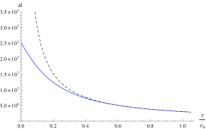
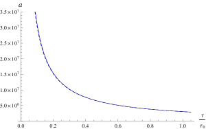
implying that in this case the De Sitter approximation used to obtain an analytical solution in the previous section is not valid as shown in fig. (1) and the numerical integration is necessary to obtain reliable results. As stated previously, we will focus on vacuum energy dominated models for which the De Sitter approximation is valid, so fig. (1) is given only to show the limits of its validity, but in all the cases we consider it turns out to be quite accurate as shown in the figures comparing analytical results, based on the De sitter approximation, and to numerical results, which take into account the small variation of the Hubble parameter. We adopt a system of units in which MPl=1subscript𝑀𝑃𝑙1M_{Pl}=1.

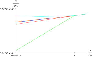
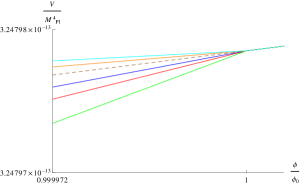
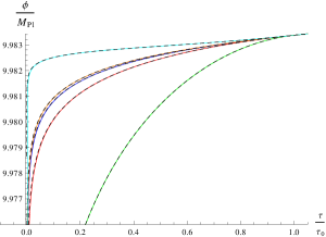
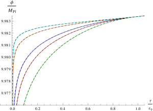
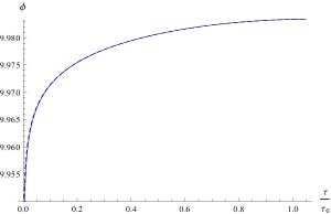
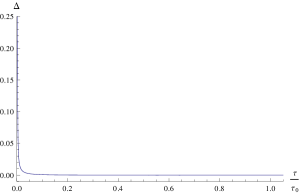
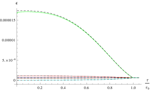
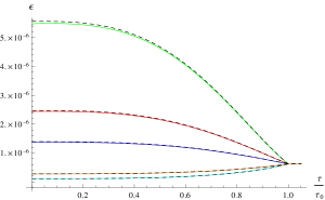
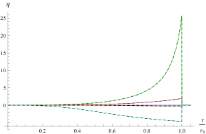
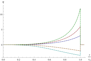
The potential as a function of the field is shown in fig. (2) for different types of features. The effects of the features on the scalar field ϕitalic-ϕ\phi and on the slow roll parameters are shown in figs. (3-6). When |λ|𝜆|\lambda| is kept constant, larger values of n𝑛n tend to produce larger variations of both ϵitalic-ϵ\epsilon and η𝜂\eta, while when n𝑛n is kept constant, larger values of |λ|𝜆|\lambda| tend to produce larger variations of both ϵitalic-ϵ\epsilon and η𝜂\eta. As it can be seen in figs. (3-4) the numerical and analytical solution for the scalar field are in a good agreement. The analytical approximation is also good for the slow roll parameters as shown in figs. (5-6). We can conclude that eq. (20) is a good approximation for the background solution within the limits of validity of the assumptions used to derive it, and we will use it in the following sections to calculate curvature perturbations. The analytical solution we derived around the time τ0subscript𝜏0\tau_{0} when the feature occurs should be accurate as long as the De sitter approximation is valid and |λ+|1much-less-thansuperscript𝜆1|\lambda^{+}|\ll 1.

Refer to caption
Refer to caption
Figure 1: Numerical (blue) and analytical (dashed black) evolution of the scale factor as a function of conformal time is plotted for n=3𝑛3n=3. On the left we choose λ=7.2×10¹⁶𝜆7.2superscript1016\lambda=7.2\times 10^{-16} and on the right λ=2.4×10¹⁸𝜆2.4superscript1018\lambda=2.4\times 10^{-18}. As it can be seen in the left plot the De Sitter approximation is not valid at late times when λϕn>V0𝜆superscriptitalic-ϕ𝑛subscript𝑉0\lambda\phi^{n}>V_{0}, so that a full numerical integration of the background equations is required, while from the right plot we can see that when λϕn<V0𝜆superscriptitalic-ϕ𝑛subscript𝑉0\lambda\phi^{n}<V_{0} the De Sitter approximation is quite accurate.
Refer to caption
Refer to caption
Figure 2: On the left the potential V𝑉V is plotted as a function of the field ϕitalic-ϕ\phi for λ=3.9×10¹⁹𝜆3.9superscript1019\lambda=3.9\times 10^{-19} and n=2/3𝑛23n=2/3 (blue), n=3𝑛3n=3 (red), and n=4𝑛4n=4 (green) and for λ=7×10²⁰𝜆7superscript1020\lambda=-7\times 10^{-20} and n=3𝑛3n=3 (orange) and n=4𝑛4n=4 (cyan). On the right the potential V𝑉V is plotted as a function of the field ϕitalic-ϕ\phi for n=3𝑛3n=3 and λ=6.0×10¹⁹𝜆6.0superscript1019\lambda=6.0\times 10^{-19} (blue), λ=1.2×10¹⁸𝜆1.2superscript1018\lambda=1.2\times 10^{-18} (red), λ=2.4×10¹⁸𝜆2.4superscript1018\lambda=2.4\times 10^{-18} (green), λ=4×10¹⁹𝜆4superscript1019\lambda=-4\times 10^{-19} (orange), and λ=7×10¹⁹𝜆7superscript1019\lambda=-7\times 10^{-19} (cyan). The dashed brown lines correspond to the potential with no feature.
Refer to caption
Refer to caption
Figure 3: On the left the numerically computed ϕitalic-ϕ\phi is plotted as a function of conformal time for λ=3.9×10¹⁹𝜆3.9superscript1019\lambda=3.9\times 10^{-19} and n=2/3𝑛23n=2/3 (blue), n=3𝑛3n=3 (red), and n=4𝑛4n=4 (green) and for λ=7×10²⁰𝜆7superscript1020\lambda=-7\times 10^{-20} and n=3𝑛3n=3 (orange) and n=4𝑛4n=4 (cyan). On the right the numerically computed ϕitalic-ϕ\phi is plotted as a function of conformal time for n=3𝑛3n=3 and λ=6.0×10¹⁹𝜆6.0superscript1019\lambda=6.0\times 10^{-19} (blue), λ=1.2×10¹⁸𝜆1.2superscript1018\lambda=1.2\times 10^{-18} (red), λ=2.4×10¹⁸𝜆2.4superscript1018\lambda=2.4\times 10^{-18} (green), λ=4×10¹⁹𝜆4superscript1019\lambda=-4\times 10^{-19} (orange), and λ=7×10¹⁹𝜆7superscript1019\lambda=-7\times 10^{-19} (cyan). The dashed black lines correspond to the analytical approximation.
Refer to caption
Refer to caption
Figure 4: On the left ϕitalic-ϕ\phi is plotted in terms of conformal time for n=4𝑛4n=4 and λ=3.9×10¹⁹𝜆3.9superscript1019\lambda=3.9\times 10^{-19}. The blue and dashed-black lines are the numerical and analytical results, respectively. On the right the relative percentage error Δ=100(ϕnumϕan)ϕnumΔ100superscriptitalic-ϕ𝑛𝑢𝑚superscriptitalic-ϕ𝑎𝑛superscriptitalic-ϕ𝑛𝑢𝑚\Delta=100\frac{(\phi^{num}-\phi^{an})}{\phi^{num}} between the numerical and analytical solutions for ϕitalic-ϕ\phi is plotted for the same values of n𝑛n and λ𝜆\lambda.
Refer to caption
Refer to caption
Figure 5: On the left the numerically computed ϵitalic-ϵ\epsilon is plotted for λ=3.9×10¹⁹𝜆3.9superscript1019\lambda=3.9\times 10^{-19} and n=2/3𝑛23n=2/3 (blue), n=3𝑛3n=3 (red), and n=4𝑛4n=4 (green) and for λ=7×10²⁰𝜆7superscript1020\lambda=-7\times 10^{-20} and n=3𝑛3n=3 (orange) and n=4𝑛4n=4 (cyan). On the right the numerically computed ϵitalic-ϵ\epsilon is plotted for n=3𝑛3n=3 and λ=6.0×10¹⁹𝜆6.0superscript1019\lambda=6.0\times 10^{-19} (blue), λ=1.2×10¹⁸𝜆1.2superscript1018\lambda=1.2\times 10^{-18} (red), λ=2.4×10¹⁸𝜆2.4superscript1018\lambda=2.4\times 10^{-18} (green), λ=4×10¹⁹𝜆4superscript1019\lambda=-4\times 10^{-19} (orange), and λ=7×10¹⁹𝜆7superscript1019\lambda=-7\times 10^{-19} (cyan). The dashed black lines correspond to the analytical approximation.
Refer to caption
Refer to caption
Figure 6: On the left the numerically computed η𝜂\eta is plotted for λ=3.9×10¹⁹𝜆3.9superscript1019\lambda=3.9\times 10^{-19} and n=2/3𝑛23n=2/3 (blue), n=3𝑛3n=3 (red), and n=4𝑛4n=4 (green) and for λ=7×10²⁰𝜆7superscript1020\lambda=-7\times 10^{-20} and n=3𝑛3n=3 (orange) and n=4𝑛4n=4 (cyan). On the right the numerically computed η𝜂\eta is plotted for n=3𝑛3n=3 and λ=6.0×10¹⁹𝜆6.0superscript1019\lambda=6.0\times 10^{-19} (blue), λ=1.2×10¹⁸𝜆1.2superscript1018\lambda=1.2\times 10^{-18} (red), λ=2.4×10¹⁸𝜆2.4superscript1018\lambda=2.4\times 10^{-18} (green), λ=4×10¹⁹𝜆4superscript1019\lambda=-4\times 10^{-19} (orange), and λ=7×10¹⁹𝜆7superscript1019\lambda=-7\times 10^{-19} (cyan). The dashed black lines correspond to the analytical approximation.

VI Spectrum of curvature perturbations

In order to study curvature perturbations we need to expand pertubatively the action respect to the background FRLW𝐹𝑅𝐿𝑊FRLW solution m ; hael . We adopt the comoving gauge in which there is no fluctuation in the scalar field, δϕ=0𝛿italic-ϕ0\delta\phi=0. The second and third order actions are respectively

S2subscript𝑆2\displaystyle S_{2} =\displaystyle= 𝑑td3x[a3ϵζ˙2aϵ(ζ)2],differential-d𝑡superscript𝑑3𝑥delimited-[]superscript𝑎3italic-ϵsuperscript˙𝜁2𝑎italic-ϵsuperscript𝜁2\displaystyle\int dtd^{3}x\left[a^{3}\epsilon\dot{\zeta}^{2}-a\epsilon(\partial\zeta)^{2}\right], (28)
S3=dtd3x[a3ϵ2ζζ˙2+aϵ2ζ(ζ)22aϵζ˙(ζ)(χ)+a3ϵ2η˙ζ2ζ˙\displaystyle S_{3}=\int dtd^{3}x\left[a^{3}\epsilon^{2}\zeta\dot{\zeta}^{2}+a\epsilon^{2}\zeta(\partial\zeta)^{2}-2a\epsilon\dot{\zeta}(\partial\zeta)(\partial\chi)+\frac{a^{3}\epsilon}{2}\dot{\eta}\zeta^{2}\dot{\zeta}\right. (29)
+ϵ2a(ζ)(χ)2χ+ϵ4a(2ζ)(χ)2+f(ζ)δLδζ|1],\displaystyle\left.+\frac{\epsilon}{2a}(\partial\zeta)(\partial\chi)\partial^{2}\chi+\frac{\epsilon}{4a}(\partial^{2}\zeta)(\partial\chi)^{2}+f(\zeta)\frac{\delta L}{\delta\zeta}\bigg{|}_{1}\right],

where

δLδζ|1evaluated-at𝛿𝐿𝛿𝜁1\displaystyle\frac{\delta L}{\delta\zeta}\bigg{|}_{1} =\displaystyle= 2a(d2χdt+H2χϵ2ζ),2𝑎𝑑superscript2𝜒𝑑𝑡𝐻superscript2𝜒italic-ϵsuperscript2𝜁\displaystyle 2a\left(\frac{d\partial^{2}\chi}{dt}+H\partial^{2}\chi-\epsilon\partial^{2}\zeta\right), (30)
f(ζ)𝑓𝜁\displaystyle f(\zeta) =\displaystyle= η4ζ+ terms with derivatives on ζ,𝜂4𝜁 terms with derivatives on 𝜁\displaystyle\frac{\eta}{4}\zeta+\mbox{ terms with derivatives on }\zeta, (31)

and δL/δζ|1evaluated-at𝛿𝐿𝛿𝜁1\delta L/\delta\zeta|_{1} is the variation of the quadratic action with respect to ζ𝜁\zeta m . The Lagrange equations for the second order action give the equation for the curvature perturbations ζ𝜁\zeta

t(a3ϵζt)aϵδij2ζxixj=0.𝑡superscript𝑎3italic-ϵ𝜁𝑡𝑎italic-ϵsuperscript𝛿𝑖𝑗superscript2𝜁superscript𝑥𝑖superscript𝑥𝑗0\frac{\partial}{\partial t}\left(a^{3}\epsilon\frac{\partial\zeta}{\partial t}\right)-a\epsilon\delta^{ij}\frac{\partial^{2}\zeta}{\partial x^{i}\partial x^{j}}=0. (32)

The Fourier transform of the above equation, using conformal time, gives

ζk′′+2zzζk+k2ζk=0,subscriptsuperscript𝜁′′𝑘2superscript𝑧𝑧subscriptsuperscript𝜁𝑘superscript𝑘2subscript𝜁𝑘0\zeta^{\prime\prime}_{k}+2\frac{z^{\prime}}{z}\zeta^{\prime}_{k}+k^{2}\zeta_{k}=0, (33)

where za2ϵ𝑧𝑎2italic-ϵz\equiv a\sqrt{2\epsilon} and k𝑘k is the comoving wave number. It is convenient to define the variable aer

uk(τ)z(τ)ζ(τ,k),subscript𝑢𝑘𝜏𝑧𝜏𝜁𝜏𝑘u_{k}(\tau)\equiv z(\tau)\zeta(\tau,k), (34)

in terms of which eq. (33) takes the form

uk′′+(k2z′′z)uk=0.superscriptsubscript𝑢𝑘′′superscript𝑘2superscript𝑧′′𝑧subscript𝑢𝑘0u_{k}^{\prime\prime}+\left(k^{2}-\frac{z^{\prime\prime}}{z}\right)u_{k}=0. (35)
Refer to caption
Refer to caption
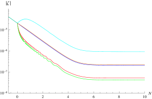
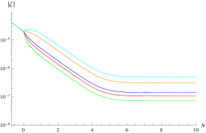
Figure 7: The numerically computed |ζk|subscript𝜁𝑘|\zeta_{k}| is plotted as a function of the number of e𝑒e-folds N𝑁N after the time of the feature. The plots on the left are for λ=3.9×10¹⁹𝜆3.9superscript1019\lambda=3.9\times 10^{-19} and n=2/3𝑛23n=2/3 (blue), n=3𝑛3n=3 (red), and n=4𝑛4n=4 (green) and for λ=7×10²⁰𝜆7superscript1020\lambda=-7\times 10^{-20} and n=3𝑛3n=3 (orange) and n=4𝑛4n=4 (cyan). The plots on the right are for n=3𝑛3n=3 and λ=6.0×10¹⁹𝜆6.0superscript1019\lambda=6.0\times 10^{-19} (blue), λ=1.2×10¹⁸𝜆1.2superscript1018\lambda=1.2\times 10^{-18} (red), λ=2.4×10¹⁸𝜆2.4superscript1018\lambda=2.4\times 10^{-18} (green), λ=4×10¹⁹𝜆4superscript1019\lambda=-4\times 10^{-19} (orange), and λ=7×10¹⁹𝜆7superscript1019\lambda=-7\times 10^{-19} (cyan). All plots are for short scale modes with k=100k0𝑘100subscript𝑘0k=100k_{0} which is sub-horizon when the feature occurs.

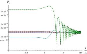
As it can be seen in fig. (7) small scales modes, which are sub-horizon at time τ0subscript𝜏0\tau_{0}, are affected by the feature. Modes that had left the horizon at that time are unaffected, since they were already frozen. In fig. (8) the power spectrum of primordial curvature perturbations Pζsubscript𝑃𝜁P_{\zeta} is plotted for different types of features.
Refer to caption
Refer to caption
Figure 8: The power spectrum of primordial curvature perturbations Pζsubscript𝑃𝜁P_{\zeta} is plotted for different types of features. The plots on the left are for λ=8×10²⁰𝜆8superscript1020\lambda=8\times 10^{-20} and n=2/3𝑛23n=2/3 (blue), n=3𝑛3n=3 (red), and n=4𝑛4n=4 (green) and for λ=5×10²⁰𝜆5superscript1020\lambda=-5\times 10^{-20} and n=3𝑛3n=3 (orange) and n=4𝑛4n=4 (cyan). For right plots n𝑛n is constant, n=3𝑛3n=3, and λ=1.0×10¹⁹𝜆1.0superscript1019\lambda=1.0\times 10^{-19} (blue), λ=5×10¹⁹𝜆5superscript1019\lambda=5\times 10^{-19} (red), λ=8×10¹⁹𝜆8superscript1019\lambda=8\times 10^{-19} (green), λ=8×10²⁰𝜆8superscript1020\lambda=-8\times 10^{-20} (orange), and λ=6×10²⁰𝜆6superscript1020\lambda=-6\times 10^{-20} (cyan). The dashed lines are the analytical approximations.
Refer to caption
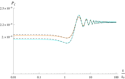
Figure 9: The power spectrum of primordial curvature perturbations Pζsubscript𝑃𝜁P_{\zeta} is plotted for n=3𝑛3n=3, λ=8×10²⁰𝜆8superscript1020\lambda=-8\times 10^{-20} (orange) and λ=6×10²⁰𝜆6superscript1020\lambda=-6\times 10^{-20} (cyan). The dashed lines are the analytical approximations. These models are able to account for the observed large scale suppression.

VII Analytical approximation for curvature perturbations

At the time of the feature there is a discontinuity in ϕ′′superscriptitalic-ϕ′′\phi^{\prime\prime} which implies that z′′superscript𝑧′′z^{\prime\prime} contains a Dirac delta function pp . We can evaluate the discontinuity in z′′/zsuperscript𝑧′′𝑧z^{\prime\prime}/z by integrating the Dirac delta function around the feature time

D0limδ0τ0δτ0+δz′′z𝑑τ=1ϕ0[ϕa0′′ϕb0′′]=nλa(τ0)2ϕ0n1ϕ0.subscript𝐷0subscript𝛿0superscriptsubscriptsubscript𝜏0𝛿subscript𝜏0𝛿superscript𝑧′′𝑧differential-d𝜏1superscriptsubscriptitalic-ϕ0delimited-[]subscriptsuperscriptitalic-ϕ′′𝑎0subscriptsuperscriptitalic-ϕ′′𝑏0𝑛𝜆𝑎superscriptsubscript𝜏02superscriptsubscriptitalic-ϕ0𝑛1superscriptsubscriptitalic-ϕ0D_{0}\equiv\lim_{\delta\to 0}\int_{\tau_{0}-\delta}^{\tau_{0}+\delta}\frac{z^{\prime\prime}}{z}d\tau=\frac{1}{\phi_{0}^{\prime}}\left[\phi^{\prime\prime}_{a0}-\phi^{\prime\prime}_{b0}\right]=-n\lambda a(\tau_{0})^{2}\frac{\phi_{0}^{n-1}}{\phi_{0}^{\prime}}. (36)

Before the feature we assume the Bunch-Davies vacuum Bunch:1978yq

v(τ,k)=eikτ2k(1ikτ).𝑣𝜏𝑘superscript𝑒i𝑘𝜏2𝑘1i𝑘𝜏v(\tau,k)=\frac{e^{-\mathrm{i}k\tau}}{\sqrt{2k}}\left(1-\frac{\mathrm{i}}{k\tau}\right). (37)

The curvature perturbations modes after the feature are approximated as a linear combination of the positive and negative frequency modes before the feature starobinsky ; Starobinsky:1998mj according to

ζ(τ,k)=1a(τ)2ϵ(τ)[α(k)v(τ,k)+β(k)v(τ,k)],𝜁𝜏𝑘1𝑎𝜏2italic-ϵ𝜏delimited-[]𝛼𝑘𝑣𝜏𝑘𝛽𝑘superscript𝑣𝜏𝑘\zeta(\tau,k)=\frac{1}{a(\tau)\sqrt{2\epsilon(\tau)}}\left[\alpha(k)v(\tau,k)+\beta(k)v^{*}(\tau,k)\right]\,, (38)

where

α(k)=1+iD0|v(τ0,k)|2 and β(k)=iD0v(τ0,k)2𝛼𝑘1isubscript𝐷0superscript𝑣subscript𝜏0𝑘2 and 𝛽𝑘isubscript𝐷0𝑣superscriptsubscript𝜏0𝑘2\alpha(k)=1+\mathrm{i}D_{0}|v(\tau_{0},k)|^{2}\>\mbox{ and }\>\beta(k)=-\mathrm{i}D_{0}v(\tau_{0},k)^{2} (39)

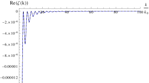
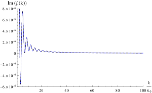
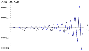
are the Bogoliubov coefficients, and τk=1/ksubscript𝜏𝑘1𝑘\tau_{k}=-1/k is the horizon crossing time for the mode k𝑘k. The coefficients α,β𝛼𝛽\alpha,\beta are determined by imposing the continuity of the modes and their derivative at the feature time pp . In figs. (10-11) we show the comparison between the numerical results for the mode function and the analytical approximation for small scales. The parameters used for the feature are n=4𝑛4n=4 and λ=3.9×10¹⁹𝜆3.9superscript1019\lambda=3.9\times 10^{-19}. In fig. (10) we show the real and imaginary part of the dependence of the mode functions on the scale and for a particular time, namely, after ten e𝑒e-folds after the feature. While in fig. (11) we show the evolution of the real and imaginary parts of the mode function at a particular scale 100k0100subscript𝑘0100k_{0}.

Refer to caption
Refer to caption
Figure 10: Numerically (blue) and analytically (black lines) computed small scale modes evaluated at 10e10𝑒10e-folds after the feature are plotted as functions of the scale. On the left it is plotted the real part, on the right the imaginary part. The parameters used for the feature are n=4𝑛4n=4 and λ=3.9×10¹⁹𝜆3.9superscript1019\lambda=3.9\times 10^{-19}.
Refer to caption
Refer to caption
Figure 11: Comparison of the evolution of the real (left) and imaginary (right) parts of the mode function for k=100k0𝑘100subscript𝑘0k=100k_{0}. The result of numerical calculations is plotted in blue, while the analytical approximation is plotted in black. The parameters used for the feature are n=4𝑛4n=4 and λ=3.9×10¹⁹𝜆3.9superscript1019\lambda=3.9\times 10^{-19}.

VIII Analytical approximation for the spectrum

The two-point function is

ζ(k1,t)ζ(k2,t)(2π)32π2k3Pζ(k)δ(3)(k1+k2),expectation𝜁subscript𝑘1𝑡𝜁subscript𝑘2𝑡superscript2𝜋32superscript𝜋2superscript𝑘3subscript𝑃𝜁𝑘superscript𝛿3subscript𝑘1subscript𝑘2\Braket{\zeta(\vec{k}_{1},t)\zeta(\vec{k}_{2},t)}\equiv(2\pi)^{3}\frac{2\pi^{2}}{k^{3}}P_{\zeta}(k)\delta^{(3)}(\vec{k}_{1}+\vec{k}_{2})\,, (40)

where the power spectrum of curvature perturbations is defined as

Pζ(k)k32π2|ζk(τe)|2,subscript𝑃𝜁𝑘superscript𝑘32superscript𝜋2superscriptsubscript𝜁𝑘subscript𝜏𝑒2P_{\zeta}(k)\equiv\frac{k^{3}}{2\pi^{2}}|\zeta_{k}(\tau_{e})|^{2}, (41)

where τesubscript𝜏𝑒\tau_{e} is the time at which inflation ends. After substituting in the above definition the analytical approximations obtained in the previous sections we get

Pζ(k)=H28π2ϵ(τe){1+D0k[(k02k21)sin(2kk0)2k0kcos(2kk0)]\displaystyle P_{\zeta}(k)=\frac{H^{2}}{8\pi^{2}\epsilon(\tau_{e})}\left\{1+\frac{D_{0}}{k}\left[\left(\frac{k_{0}^{2}}{k^{2}}-1\right)\sin\left(\frac{2k}{k_{0}}\right)-\frac{2k_{0}}{k}\cos\left(\frac{2k}{k_{0}}\right)\right]\right.
(42)
+D022k2[1+2k02k2+k04k4+(1k04k4)cos(2kk0)2k0k(1+k02k2)sin(2kk0)]}.\displaystyle\left.+\frac{D_{0}^{2}}{2k^{2}}\left[1+\frac{2k_{0}^{2}}{k^{2}}+\frac{k_{0}^{4}}{k^{4}}+\left(1-\frac{k_{0}^{4}}{k^{4}}\right)\cos\left(\frac{2k}{k_{0}}\right)-\frac{2k_{0}}{k}\left(1+\frac{k_{0}^{2}}{k^{2}}\right)\sin\left(\frac{2k}{k_{0}}\right)\right]\right\}\,.

This generalizes the result obtained in starobinsky for a potential with a discontinuous first derivative to the more general case considered in this paper, corresponding to eq. (36). In fig. (8) we compare the analytical expression for the power spectrum given by eq. (VIII) with the numerical results obtained by integrating numerically both the background and the perturbations equations. The analytical result is quite accurate and it improves the results obtained in aer because we use the analytical approximation for the perturbations modes also for modes which were superhorizon slightly before τ0subscript𝜏0\tau_{0}, improving substantially the agreement with numerical results. This is due to the well known fact that modes are not completely frozen at τk=1/ksubscript𝜏𝑘1𝑘\tau_{k}=-1/k, but keep evolving for few e-folds after, so that also scales slightly greater than k0subscript𝑘0k_{0} are mildly affected by the features.

It should be noted that the formula (VIII) we obtained is not depending on the slow-roll approximation, since it is derived directly from the definition of the power spectrum in eq. (41), and this explains why it is in such a good agreement with fully numerical calculations despite the temporary violation of slow-roll regime produced by the features. The ϵitalic-ϵ\epsilon in the denominator of eq. (VIII) comes in fact from the analytical solution for the perturbation modes, which is not based on any slow-roll expansion because it comes from za2ϵ𝑧𝑎2italic-ϵz\equiv a\sqrt{2\epsilon} in eqs. (33,35) which are valid at any order in slow-roll.

As can be seen in fig. (8) negative values of λ𝜆\lambda correspond to a suppression of the spectrum on large and intermediate scales, while positive values produce a suppression on small scales. While the analysis of observational data goes beyond the scope of this paper, we can see in fig. (8) that an appropriate choice of parameters gives spectra in good qualitative agreement with the features recently found when parameterizing the free primordial power spectrum with a piecewise cubic Hermite interpolating polynomial Gariazzo:2014dla .

IX Calculation of the bispectrum

The Fourier transform of the three-point correlation function pxxii ; pxxiv , also known as the bispectrum Bζsubscript𝐵𝜁B_{\zeta} is given by

ζ(k1,t)ζ(k2,t)ζ(k3,t)=(2π)3Bζ(k1,k2,k3)δ(3)(k1+k2,k3),expectation𝜁subscript𝑘1𝑡𝜁subscript𝑘2𝑡𝜁subscript𝑘3𝑡superscript2𝜋3subscript𝐵𝜁subscript𝑘1subscript𝑘2subscript𝑘3superscript𝛿3subscript𝑘1subscript𝑘2subscript𝑘3\Braket{\zeta(\vec{k}_{1},t)\zeta(\vec{k}_{2},t)\zeta(\vec{k}_{3},t)}=(2\pi)^{3}B_{\zeta}(k_{1},k_{2},k_{3})\delta^{(3)}(\vec{k}_{1}+\vec{k}_{2},\vec{k}_{3}), (43)

and it should vanish if the curvature perturbations are Gaussian xc ; a2 . Therefore, deviations from non Gaussianity can be determined by measuring the implications of a non vanishing Bζsubscript𝐵𝜁B_{\zeta} on the CMB radiation. Following the procedure in Ref. aer , after a field redefinition, the third order action can be written as

S3=𝑑td3x[a3ϵηζζ˙212aϵηζ2ζ].subscript𝑆3differential-d𝑡superscript𝑑3𝑥delimited-[]superscript𝑎3italic-ϵ𝜂𝜁superscript˙𝜁212𝑎italic-ϵ𝜂𝜁superscript2𝜁S_{3}=\int dtd^{3}x\left[-a^{3}\epsilon\eta\zeta\dot{\zeta}^{2}-\frac{1}{2}a\epsilon\eta\zeta\partial^{2}\zeta\right]. (44)

From this action the interaction Hamiltonian can be written in terms of conformal time as

Hint(τ)=d3xϵηa[ζζ+212ζ22ζ].\displaystyle H_{int}(\tau)=\int d^{3}x\,\epsilon\eta a\left[\zeta\zeta^{\prime}{}^{2}+\frac{1}{2}\zeta^{2}\partial^{2}\zeta\right]. (45)

The 3-point correlation function is given by m ; xc

Ω|ζ(τe,k1)ζ(τe,k2)ζ(τe,k3)|Ω=iτe0|[ζ(τe,k1)ζ(τe,k2)ζ(τe,k3),Hint]|0,quantum-operator-productΩ𝜁subscript𝜏𝑒subscript𝑘1𝜁subscript𝜏𝑒subscript𝑘2𝜁subscript𝜏𝑒subscript𝑘3Ωisuperscriptsubscriptsubscript𝜏𝑒quantum-operator-product0𝜁subscript𝜏𝑒subscript𝑘1𝜁subscript𝜏𝑒subscript𝑘2𝜁subscript𝜏𝑒subscript𝑘3subscript𝐻𝑖𝑛𝑡0\displaystyle\Braket{\Omega}{\zeta(\tau_{e},\vec{k}_{1})\zeta(\tau_{e},\vec{k}_{2})\zeta(\tau_{e},\vec{k}_{3})}{\Omega}=-\mathrm{i}\int_{-\infty}^{\tau_{e}}\Braket{0}{\left[\zeta(\tau_{e},\vec{k}_{1})\zeta(\tau_{e},\vec{k}_{2})\zeta(\tau_{e},\vec{k}_{3}),H_{int}\right]}{0}, (46)

and after substitution the expression for the bispectrum Bζsubscript𝐵𝜁B_{\zeta} inin ; xc is

Bζ(k1,k2,k3)=2[ζ(τe,k1)ζ(τe,k2)ζ(τe,k3)τ0τedτηϵa2(2ζ(τ,k1)ζ(τ,k2)ζ(τ,k3)\displaystyle B_{\zeta}(k_{1},k_{2},k_{3})=2\Im\Bigl{[}\zeta(\tau_{e},k_{1})\zeta(\tau_{e},k_{2})\zeta(\tau_{e},k_{3})\int^{\tau_{e}}_{\tau_{0}}d\tau\eta\epsilon a^{2}\biggl{(}2\zeta^{*}(\tau,k_{1})\zeta^{\prime}{}^{*}(\tau,k_{2})\zeta^{\prime}{}^{*}(\tau,k_{3}) (47)
k12ζ(τ,k1)ζ(τ,k2)ζ(τ,k3))+ two permutations of k1,k2, and k3],\displaystyle-k^{2}_{1}\zeta^{*}(\tau,k_{1})\zeta^{*}(\tau,k_{2})\zeta^{*}(\tau,k_{3})\biggr{)}+\mbox{ two permutations of }k_{1},k_{2},\mbox{ and }k_{3}\Bigr{]}\,,

where \Im is the imaginary part and we evaluate the integral from τ0subscript𝜏0\tau_{0} to τesubscript𝜏𝑒\tau_{e}, where τesubscript𝜏𝑒\tau_{e} is some time sufficiently after Hubble crossing horizon, when the modes are frozen a1 ; a2 ; a3 ; bingo ; numerical2013 .

It is common to study non-Gaussianity using the parameter fNLsubscript𝑓𝑁𝐿f_{NL} defined by

65fNL(k1,k2,k3)Bζ𝐏ζ(k1)𝐏ζ(k2)+𝐏ζ(k1)𝐏ζ(k3)+𝐏ζ(k2)𝐏ζ(k3),65subscript𝑓𝑁𝐿subscript𝑘1subscript𝑘2subscript𝑘3subscript𝐵𝜁subscript𝐏𝜁subscript𝑘1subscript𝐏𝜁subscript𝑘2subscript𝐏𝜁subscript𝑘1subscript𝐏𝜁subscript𝑘3subscript𝐏𝜁subscript𝑘2subscript𝐏𝜁subscript𝑘3\displaystyle\frac{6}{5}f_{NL}(k_{1},k_{2},k_{3})\equiv\frac{B_{\zeta}}{\mathbf{P}_{\zeta}(k_{1})\mathbf{P}_{\zeta}(k_{2})+\mathbf{P}_{\zeta}(k_{1})\mathbf{P}_{\zeta}(k_{3})+\mathbf{P}_{\zeta}(k_{2})\mathbf{P}_{\zeta}(k_{3})}\,, (48)

where

𝐏ζ2π2k3Pζ,subscript𝐏𝜁2superscript𝜋2superscript𝑘3subscript𝑃𝜁\mathbf{P}_{\zeta}\equiv\frac{2\pi^{2}}{k^{3}}P_{\zeta}\,, (49)

Replacing 𝐏ζsubscript𝐏𝜁\mathbf{P}_{\zeta} in eq.(48) we obtain fNLsubscript𝑓𝑁𝐿f_{NL} in terms of our dimensionless definition of the spectrum Pζ(k)subscript𝑃𝜁𝑘P_{\zeta}(k)

fNL(k1,k2,k3)=103(k1k2k3)3(2π)4BζPζ(k1)Pζ(k2)k33+Pζ(k1)Pζ(k3)k23+Pζ(k2)Pζ(k3)k13.subscript𝑓𝑁𝐿subscript𝑘1subscript𝑘2subscript𝑘3103superscriptsubscript𝑘1subscript𝑘2subscript𝑘33superscript2𝜋4subscript𝐵𝜁subscript𝑃𝜁subscript𝑘1subscript𝑃𝜁subscript𝑘2subscriptsuperscript𝑘33subscript𝑃𝜁subscript𝑘1subscript𝑃𝜁subscript𝑘3subscriptsuperscript𝑘32subscript𝑃𝜁subscript𝑘2subscript𝑃𝜁subscript𝑘3subscriptsuperscript𝑘31\displaystyle f_{NL}(k_{1},k_{2},k_{3})=\frac{10}{3}\frac{(k_{1}k_{2}k_{3})^{3}}{(2\pi)^{4}}\frac{B_{\zeta}}{P_{\zeta}(k_{1})P_{\zeta}(k_{2})k^{3}_{3}+P_{\zeta}(k_{1})P_{\zeta}(k_{3})k^{3}_{2}+P_{\zeta}(k_{2})P_{\zeta}(k_{3})k^{3}_{1}}\,. (50)

In this paper we will study non-Gaussianity using a different quantity defined as

FNL(k1,k2,k3;k)103(2π)4(k1k2k3)3k13+k23+k33Bζ(k1,k2,k3)Pζ2(k),subscript𝐹𝑁𝐿subscript𝑘1subscript𝑘2subscript𝑘3subscript𝑘103superscript2𝜋4superscriptsubscript𝑘1subscript𝑘2subscript𝑘33superscriptsubscript𝑘13superscriptsubscript𝑘23superscriptsubscript𝑘33subscript𝐵𝜁subscript𝑘1subscript𝑘2subscript𝑘3superscriptsubscript𝑃𝜁2subscript𝑘F_{NL}(k_{1},k_{2},k_{3};k_{*})\equiv\frac{10}{3(2\pi)^{4}}\frac{(k_{1}k_{2}k_{3})^{3}}{k_{1}^{3}+k_{2}^{3}+k_{3}^{3}}\frac{B_{\zeta}(k_{1},k_{2},k_{3})}{P_{\zeta}^{2}(k_{*})}\,, (51)

where ksubscript𝑘k_{*} is a pivot scale at which the power spectrum is evaluated which corresponds approximately to the scale of normalization of the spectrum, i.e. Pζ(k)2.2×10⁹subscript𝑃𝜁subscript𝑘2.2superscript109P_{\zeta}(k_{*})\approx 2.2\times 10^{-9}. Our definition of FNLsubscript𝐹𝑁𝐿F_{NL} reduces to fNLsubscript𝑓𝑁𝐿f_{NL} in the equilateral limit if the spectrum is approximately scale invariant, but in general fNLsubscript𝑓𝑁𝐿f_{NL} and FNLsubscript𝐹𝑁𝐿F_{NL} are different, and for example in the squeezed limit they are not the same. For this reason they cannot be compared directly but FNLsubscript𝐹𝑁𝐿F_{NL} still provides useful information about the non-Gaussian behavior of Bζsubscript𝐵𝜁B_{\zeta}.

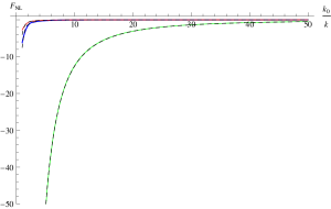
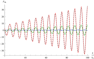
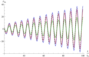
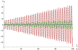
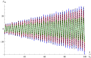
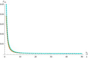
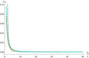
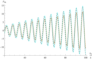
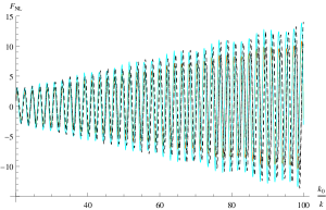
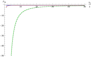
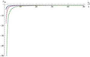
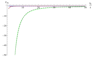
In figs. (12-13) the large scale squeezed and equilateral limit of the bispectrum are plotted for different values of the parameters n𝑛n and λ𝜆\lambda. The small scale squeezed and equilateral limits are shown in figs. (14) and (15), respectively. As shown in figs. (14-15) the bispectrum has an oscillatory behavior with an amplitude inversely proportional to the scale.
Refer to caption
Refer to caption
Figure 12: The squeezed limit of the numerically computed bispectrum FNL(k0/500,k,k)subscript𝐹𝑁𝐿subscript𝑘0500𝑘𝑘F_{NL}(k_{0}/500,k,k) in plotted for a large scale k0/500subscript𝑘0500k_{0}/500. On the left we keep λ𝜆\lambda constant, λ=3.9×10¹⁹𝜆3.9superscript1019\lambda=3.9\times 10^{-19}, while n=2/3𝑛23n=2/3 (blue), n=3𝑛3n=3 (red), and n=4𝑛4n=4 (green). On the right we keep n𝑛n constant, n=3𝑛3n=3, while λ=6.0×10¹⁹𝜆6.0superscript1019\lambda=6.0\times 10^{-19} (blue), λ=1.2×10¹⁸𝜆1.2superscript1018\lambda=1.2\times 10^{-18} (red), and λ=2.4×10¹⁸𝜆2.4superscript1018\lambda=2.4\times 10^{-18} (green). The dashed black lines correspond to the analytical approximation.
Refer to caption
Refer to caption
Figure 13: The equilateral limit of the numerically computed bispectrum FNL(k,k,k)subscript𝐹𝑁𝐿𝑘𝑘𝑘F_{NL}(k,k,k) in plotted for large scales. On the left we keep λ𝜆\lambda constant, λ=3.9×10¹⁹𝜆3.9superscript1019\lambda=3.9\times 10^{-19}, while n=2/3𝑛23n=2/3 (blue), n=3𝑛3n=3 (red), and n=4𝑛4n=4 (green). On the right we keep n𝑛n constant, n=3𝑛3n=3, while λ=6.0×10¹⁹𝜆6.0superscript1019\lambda=6.0\times 10^{-19} (blue), λ=1.2×10¹⁸𝜆1.2superscript1018\lambda=1.2\times 10^{-18} (red), and λ=2.4×10¹⁸𝜆2.4superscript1018\lambda=2.4\times 10^{-18} (green). The dashed black lines correspond to the analytical approximation.
Refer to caption
Refer to caption
Figure 14: The squeezed limit of the numerically computed bispectrum FNL(k,1000k0,1000k0)subscript𝐹𝑁𝐿𝑘1000subscript𝑘01000subscript𝑘0F_{NL}(k,1000k_{0},1000k_{0}) is plotted for a small scale 1000k01000subscript𝑘01000k_{0}. On the left λ𝜆\lambda is constant, λ=3.9×10¹⁹𝜆3.9superscript1019\lambda=3.9\times 10^{-19}, while n=2/3𝑛23n=2/3 (blue), n=3𝑛3n=3 (red), and n=4𝑛4n=4 (green). On the right n𝑛n is constant, n=3𝑛3n=3, while λ=6.0×10¹⁹𝜆6.0superscript1019\lambda=6.0\times 10^{-19} (blue), λ=1.2×10¹⁸𝜆1.2superscript1018\lambda=1.2\times 10^{-18} (red), and λ=2.4×10¹⁸𝜆2.4superscript1018\lambda=2.4\times 10^{-18} (green). The dashed black lines correspond to the analytical approximation.
Refer to caption
Refer to caption
Figure 15: The equilateral limit of the numerically computed bispectrum FNL(k,k,k)subscript𝐹𝑁𝐿𝑘𝑘𝑘F_{NL}(k,k,k) is plotted for small scales. On the left λ𝜆\lambda is constant, λ=3.9×10¹⁹𝜆3.9superscript1019\lambda=3.9\times 10^{-19}, while n=2/3𝑛23n=2/3 (blue), n=3𝑛3n=3 (red), and n=4𝑛4n=4 (green). On the right n𝑛n is constant, n=3𝑛3n=3, while λ=6.0×10¹⁹𝜆6.0superscript1019\lambda=6.0\times 10^{-19} (blue), λ=1.2×10¹⁸𝜆1.2superscript1018\lambda=1.2\times 10^{-18} (red), and λ=2.4×10¹⁸𝜆2.4superscript1018\lambda=2.4\times 10^{-18} (green). The dashed black lines correspond to the analytical approximation.

X Analytical approximation for the bispectrum

In order to obtain an analytical approximation for the bispectrum we use eq. (38) for curvature perturbations and eq. (25) for slow-roll parameters. This implies that also the different approximations are used in different cases as explained in more details in the following sections. All the results presented in this section should be considered taking into account the existence of a cut-off scales beyond which the Heaviside approximation of a smooth transition is not valid as discussed in more details in aer ; pp . We provide analytical expressions for the bispectrum for different types of features, i.e., different values of n𝑛n and λ𝜆\lambda, in the squeezed and equilateral limit for both large and small scales. The analytical results are shown in dashed black lines in figs. (12-15) where it can be seen that the approximations for the bispectrum are in good agreement with the numerical results.

X.1 Large scales

In the large scale limit when ki<k0,i=1,2,3formulae-sequencesubscript𝑘𝑖subscript𝑘0𝑖123k_{i}<k_{0},\,i=1,2,3, the curvature perturbations modes are frozen in the time interval of interest, since there is no time evolution for τ>τ0>τki𝜏subscript𝜏0subscript𝜏subscript𝑘𝑖\tau>\tau_{0}>\tau_{k_{i}}. Thus in eq. (47) all the modes functions can be evaluated at τ0subscript𝜏0\tau_{0} and pulled out of the integrals while the terms ζ(τ,ki)\zeta^{\prime}{}^{*}(\tau,k_{i}) can be set to zero. Following this approximation we get

FNL<(k1,k2,k3)20(i=13ki3)3(2π)4Pζ2(k)i=13ki2i=13ki3[i=13ζ(τe,ki)ζ(τ0,ki)]τ0τe𝑑τηϵa2superscriptsubscript𝐹𝑁𝐿subscript𝑘1subscript𝑘2subscript𝑘320superscriptsubscriptproduct𝑖13superscriptsubscript𝑘𝑖33superscript2𝜋4superscriptsubscript𝑃𝜁2subscript𝑘superscriptsubscript𝑖13superscriptsubscript𝑘𝑖2superscriptsubscript𝑖13superscriptsubscript𝑘𝑖3superscriptsubscriptproduct𝑖13𝜁subscript𝜏𝑒subscript𝑘𝑖superscript𝜁subscript𝜏0subscript𝑘𝑖subscriptsuperscriptsubscript𝜏𝑒subscript𝜏0differential-d𝜏𝜂italic-ϵsuperscript𝑎2\displaystyle F_{NL}^{<}(k_{1},k_{2},k_{3})\approx\frac{-20(\prod_{i=1}^{3}k_{i}^{3})}{3(2\pi)^{4}P_{\zeta}^{2}(k_{*})}\frac{\sum_{i=1}^{3}k_{i}^{2}}{\sum_{i=1}^{3}k_{i}^{3}}\Im\left[\prod_{i=1}^{3}\zeta(\tau_{e},k_{i})\zeta^{*}(\tau_{0},k_{i})\right]\int^{\tau_{e}}_{\tau_{0}}d\tau\eta\epsilon a^{2} (52)
20(i=13ki3)3(2π)4Pζ2(k)i=13ki2i=13ki3ϕa+2(λ+)3a(τe)H[i=13ζ(τe,ki)ζ(τ0,ki)],absent20superscriptsubscriptproduct𝑖13superscriptsubscript𝑘𝑖33superscript2𝜋4superscriptsubscript𝑃𝜁2subscript𝑘superscriptsubscript𝑖13superscriptsubscript𝑘𝑖2superscriptsubscript𝑖13superscriptsubscript𝑘𝑖3superscriptsubscriptitalic-ϕ𝑎2superscriptsuperscript𝜆3𝑎subscript𝜏𝑒𝐻superscriptsubscriptproduct𝑖13𝜁subscript𝜏𝑒subscript𝑘𝑖superscript𝜁subscript𝜏0subscript𝑘𝑖\displaystyle\approx\frac{-20(\prod_{i=1}^{3}k_{i}^{3})}{3(2\pi)^{4}P_{\zeta}^{2}(k_{*})}\frac{\sum_{i=1}^{3}k_{i}^{2}}{\sum_{i=1}^{3}k_{i}^{3}}\frac{\phi_{a}^{+2}(\lambda^{+})^{3}a(\tau_{e})}{H}\Im\left[\prod_{i=1}^{3}\zeta(\tau_{e},k_{i})\zeta^{*}(\tau_{0},k_{i})\right]\,,

where we have used the approximations for the slow-roll parameters in eq. (25) in the integration. Now we use the analytical approximations for the perturbation to obtain at large scales

FNL<(k1,k2,k3)56H5(2π)4Pζ2(k)ϕa+2a(τe)(λ+)3(ϕb+)6i=13ki2i=13ki3[i=13(τekii)(kiτ0+i)ei(k1+k2+k3)τ0].superscriptsubscript𝐹𝑁𝐿subscript𝑘1subscript𝑘2subscript𝑘356superscript𝐻5superscript2𝜋4superscriptsubscript𝑃𝜁2subscript𝑘superscriptsubscriptitalic-ϕ𝑎2𝑎subscript𝜏𝑒superscriptsuperscript𝜆3superscriptsuperscriptsubscriptitalic-ϕ𝑏6superscriptsubscript𝑖13superscriptsubscript𝑘𝑖2superscriptsubscript𝑖13superscriptsubscript𝑘𝑖3superscriptsubscriptproduct𝑖13subscript𝜏𝑒subscript𝑘𝑖isubscript𝑘𝑖subscript𝜏0isuperscript𝑒isubscript𝑘1subscript𝑘2subscript𝑘3subscript𝜏0\displaystyle F_{NL}^{<}(k_{1},k_{2},k_{3})\approx-\frac{5}{6}\frac{H^{5}}{(2\pi)^{4}P_{\zeta}^{2}(k_{*})}\frac{\phi_{a}^{+2}a(\tau_{e})}{(\lambda^{+})^{3}(\phi_{b}^{+})^{6}}\frac{\sum_{i=1}^{3}k_{i}^{2}}{\sum_{i=1}^{3}k_{i}^{3}}\Im\left[\prod_{i=1}^{3}(\tau_{e}k_{i}-\mathrm{i})(k_{i}\tau_{0}+\mathrm{i})e^{\mathrm{i}(k_{1}+k_{2}+k_{3})\tau_{0}}\right]\,. (53)

In the squeezed limit with k1k2=k3kmuch-less-thansubscript𝑘1subscript𝑘2subscript𝑘3𝑘k_{1}\ll k_{2}=k_{3}\equiv k and k<k0𝑘subscript𝑘0k<k_{0} this expression reduces to the following analytical formula

FNL<SL(k1,k)56H5(2π)4Pζ2(k)ϕa+2a(τe)(λ+)3(ϕb+)61k[2k+k1k0cos(2k+k1k0)\displaystyle F_{NL}^{<SL}(k_{1},k)\approx-\frac{5}{6}\frac{H^{5}}{(2\pi)^{4}P_{\zeta}^{2}(k_{*})}\frac{\phi_{a}^{+2}a(\tau_{e})}{(\lambda^{+})^{3}(\phi_{b}^{+})^{6}}\frac{1}{k}\Biggl{[}\frac{2k+k_{1}}{k_{0}}\cos{\left(\frac{2k+k_{1}}{k_{0}}\right)} (54)
+(kk02k1+kk01)sin(2k+k1k0)].\displaystyle+\left(\frac{k}{k_{0}}\frac{2k_{1}+k}{k_{0}}-1\right)\sin{\left(\frac{2k+k_{1}}{k_{0}}\right)}\Biggr{]}\,.

As shown in fig. (12) the analytical approximation is in good agreement with the numerical results. Here and in any other approximation for the FNLsubscript𝐹𝑁𝐿F_{NL} as defined in eq. (51) we use eq. (VIII) for the spectrum Pζsubscript𝑃𝜁P_{\zeta}.

In the large scale equilateral limit, when k1=k2=k3kk0subscript𝑘1subscript𝑘2subscript𝑘3𝑘much-less-thansubscript𝑘0k_{1}=k_{2}=k_{3}\equiv k\ll k_{0} eq. (53) becomes

FNL<EL(k)56H5(2π)4Pζ2(k)ϕa+2a(τe)(λ+)3(ϕb+)61k[3kk0cos(3kk0)+(3k2k021)sin(3kk0)].superscriptsubscript𝐹𝑁𝐿absent𝐸𝐿𝑘56superscript𝐻5superscript2𝜋4superscriptsubscript𝑃𝜁2subscript𝑘superscriptsubscriptitalic-ϕ𝑎2𝑎subscript𝜏𝑒superscriptsuperscript𝜆3superscriptsuperscriptsubscriptitalic-ϕ𝑏61𝑘delimited-[]3𝑘subscript𝑘03𝑘subscript𝑘03superscript𝑘2superscriptsubscript𝑘0213𝑘subscript𝑘0\displaystyle F_{NL}^{<EL}(k)\approx-\frac{5}{6}\frac{H^{5}}{(2\pi)^{4}P_{\zeta}^{2}(k_{*})}\frac{\phi_{a}^{+2}a(\tau_{e})}{(\lambda^{+})^{3}(\phi_{b}^{+})^{6}}\frac{1}{k}\left[\frac{3k}{k_{0}}\cos{\left(\frac{3k}{k_{0}}\right)}+\left(\frac{3k^{2}}{k_{0}^{2}}-1\right)\sin{\left(\frac{3k}{k_{0}}\right)}\right]\,. (55)

Numerical result and eq. (55) are in good agreement as shown in fig. (13). In figs. (12-13) we have evaluated both the numerical and analytical expressions at a time τesubscript𝜏𝑒\tau_{e} corresponding approximately to 10e10𝑒10e-folds after the feature a1 ; a2 ; bingo ; numerical2013 . As can be seen in figs. (12-13) the large scale bispectrum in the squeezed and equilateral limits have a very similar form and are linearly suppressed.

X.2 Small scales

In the small scale limit, when ki>k0subscript𝑘𝑖subscript𝑘0k_{i}>k_{0}, it is convenient to re-write the expression for FNLsubscript𝐹𝑁𝐿F_{NL} as

FNL>(k1,k2,k3)203(2π)4(k1k2k3)3k13+k23+k331Pζ2(k)[ζ(τe,k1)ζ(τe,k2)ζ(τe,k3)(2I1(k1,k2,k3)\displaystyle F_{NL}^{>}(k_{1},k_{2},k_{3})\approx\frac{20}{3(2\pi)^{4}}\frac{(k_{1}k_{2}k_{3})^{3}}{k_{1}^{3}+k_{2}^{3}+k_{3}^{3}}\frac{1}{P_{\zeta}^{2}(k_{*})}\Im\biggl{[}\zeta(\tau_{e},k_{1})\zeta(\tau_{e},k_{2})\zeta(\tau_{e},k_{3})\biggl{(}2I_{1}(k_{1},k_{2},k_{3}) (56)
k12I2(k1,k2,k3))+ two permutations of k1,k2, and k3],\displaystyle-k_{1}^{2}I_{2}(k_{1},k_{2},k_{3})\biggr{)}+\mbox{ two permutations of }k_{1},k_{2},\mbox{ and }k_{3}\biggr{]}\,,

where

I1(k1,k2,k3)τ0τedτη(τ)ϵ(τ)a(τ)2ζ(τ,k1)ζ(τ,k2)ζ(τ,k3)\displaystyle I_{1}(k_{1},k_{2},k_{3})\equiv\int^{\tau_{e}}_{\tau_{0}}d\tau\,\eta(\tau)\epsilon(\tau)a(\tau)^{2}\zeta^{*}(\tau,k_{1})\zeta^{\prime}{}^{*}(\tau,k_{2})\zeta^{\prime}{}^{*}(\tau,k_{3}) (57)
τ0τedτ[λ+(λ)2ϕa+ϕaa(τ)2+λ+(λ)3(ϕa)2a(τ)2+2λ]ζ(τ,k1)ζ(τ,k2)ζ(τ,k3),\displaystyle\approx\int^{\tau_{e}}_{\tau_{0}}d\tau\Bigl{[}\lambda^{+}(\lambda^{-})^{2}\phi_{a}^{+}\phi_{a}^{-}a(\tau)^{2+\lambda^{-}}+(\lambda^{-})^{3}(\phi_{a}^{-})^{2}a(\tau)^{2+2\lambda^{-}}\Bigr{]}\zeta^{*}(\tau,k_{1})\zeta^{\prime}{}^{*}(\tau,k_{2})\zeta^{\prime}{}^{*}(\tau,k_{3})\,,
I2(k1,k2,k3)τ0τe𝑑τη(τ)ϵ(τ)a(τ)2ζ(τ,k1)ζ(τ,k2)ζ(τ,k3)subscript𝐼2subscript𝑘1subscript𝑘2subscript𝑘3subscriptsuperscriptsubscript𝜏𝑒subscript𝜏0differential-d𝜏𝜂𝜏italic-ϵ𝜏𝑎superscript𝜏2superscript𝜁𝜏subscript𝑘1superscript𝜁𝜏subscript𝑘2superscript𝜁𝜏subscript𝑘3\displaystyle I_{2}(k_{1},k_{2},k_{3})\equiv\int^{\tau_{e}}_{\tau_{0}}d\tau\,\eta(\tau)\epsilon(\tau)a(\tau)^{2}\zeta^{*}(\tau,k_{1})\zeta^{*}(\tau,k_{2})\zeta^{*}(\tau,k_{3}) (58)
=τ0τe𝑑τ[λ+(λ)2ϕa+ϕaa(τ)2+λ+(λ)3(ϕa)2a(τ)2+2λ]ζ(τ,k1)ζ(τ,k2)ζ(τ,k3).absentsubscriptsuperscriptsubscript𝜏𝑒subscript𝜏0differential-d𝜏delimited-[]superscript𝜆superscriptsuperscript𝜆2superscriptsubscriptitalic-ϕ𝑎superscriptsubscriptitalic-ϕ𝑎𝑎superscript𝜏2superscript𝜆superscriptsuperscript𝜆3superscriptsuperscriptsubscriptitalic-ϕ𝑎2𝑎superscript𝜏22superscript𝜆superscript𝜁𝜏subscript𝑘1superscript𝜁𝜏subscript𝑘2superscript𝜁𝜏subscript𝑘3\displaystyle=\int^{\tau_{e}}_{\tau_{0}}d\tau\Bigl{[}\lambda^{+}(\lambda^{-})^{2}\phi_{a}^{+}\phi_{a}^{-}a(\tau)^{2+\lambda^{-}}+(\lambda^{-})^{3}(\phi_{a}^{-})^{2}a(\tau)^{2+2\lambda^{-}}\Bigr{]}\zeta^{*}(\tau,k_{1})\zeta^{*}(\tau,k_{2})\zeta^{*}(\tau,k_{3})\,.

In the above expressions we have used eq. (25) to derive an approximation for ηϵa2𝜂italic-ϵsuperscript𝑎2\eta\epsilon a^{2} as

ηϵa2=[(λ+)2ϕa+aλ++(λ)2ϕaaλ][λ+ϕa+aλ++λϕaaλ]a2𝜂italic-ϵsuperscript𝑎2delimited-[]superscriptsuperscript𝜆2superscriptsubscriptitalic-ϕ𝑎superscript𝑎superscript𝜆superscriptsuperscript𝜆2superscriptsubscriptitalic-ϕ𝑎superscript𝑎superscript𝜆delimited-[]superscript𝜆superscriptsubscriptitalic-ϕ𝑎superscript𝑎superscript𝜆superscript𝜆superscriptsubscriptitalic-ϕ𝑎superscript𝑎superscript𝜆superscript𝑎2\displaystyle\eta\epsilon a^{2}=\left[(\lambda^{+})^{2}\phi_{a}^{+}a^{\lambda^{+}}+(\lambda^{-})^{2}\phi_{a}^{-}a^{\lambda^{-}}\right]\left[\lambda^{+}\phi_{a}^{+}a^{\lambda^{+}}+\lambda^{-}\phi_{a}^{-}a^{\lambda^{-}}\right]a^{2} (59)
=[(λ+)3(ϕa+)2a2λ++(λ++λ)λ+λϕa+ϕaaλ++λ+(λ)3(ϕa)2a2λ]a2absentdelimited-[]superscriptsuperscript𝜆3superscriptsuperscriptsubscriptitalic-ϕ𝑎2superscript𝑎2superscript𝜆superscript𝜆superscript𝜆superscript𝜆superscript𝜆superscriptsubscriptitalic-ϕ𝑎superscriptsubscriptitalic-ϕ𝑎superscript𝑎superscript𝜆superscript𝜆superscriptsuperscript𝜆3superscriptsuperscriptsubscriptitalic-ϕ𝑎2superscript𝑎2superscript𝜆superscript𝑎2\displaystyle=\left[(\lambda^{+})^{3}(\phi_{a}^{+})^{2}a^{2\lambda^{+}}+(\lambda^{+}+\lambda^{-})\lambda^{+}\lambda^{-}\phi_{a}^{+}\phi_{a}^{-}a^{\lambda^{+}+\lambda^{-}}+(\lambda^{-})^{3}(\phi_{a}^{-})^{2}a^{2\lambda^{-}}\right]a^{2}
λ+(λ)2ϕa+ϕaa2+λ+(λ)3(ϕa)2a2+2λ.absentsuperscript𝜆superscriptsuperscript𝜆2superscriptsubscriptitalic-ϕ𝑎superscriptsubscriptitalic-ϕ𝑎superscript𝑎2superscript𝜆superscriptsuperscript𝜆3superscriptsuperscriptsubscriptitalic-ϕ𝑎2superscript𝑎22superscript𝜆\displaystyle\approx\lambda^{+}(\lambda^{-})^{2}\phi_{a}^{+}\phi_{a}^{-}a^{2+\lambda^{-}}+(\lambda^{-})^{3}(\phi_{a}^{-})^{2}a^{2+2\lambda^{-}}\,.

All the integrals we need to compute have a similar form, so it is useful to re-write eqs. (57) and (58) as

Ii(k1,k2,k3)[λ+(λ)2ϕa+ϕa𝒜i(τ,k1,k2,k3,q1)+(λ)3(ϕa)2𝒜i(τ,k1,k2,k3,q2)]|τ0τesubscript𝐼𝑖subscript𝑘1subscript𝑘2subscript𝑘3evaluated-atdelimited-[]superscript𝜆superscriptsuperscript𝜆2superscriptsubscriptitalic-ϕ𝑎superscriptsubscriptitalic-ϕ𝑎subscript𝒜𝑖𝜏subscript𝑘1subscript𝑘2subscript𝑘3subscript𝑞1superscriptsuperscript𝜆3superscriptsuperscriptsubscriptitalic-ϕ𝑎2subscript𝒜𝑖𝜏subscript𝑘1subscript𝑘2subscript𝑘3subscript𝑞2subscript𝜏0subscript𝜏𝑒\displaystyle I_{i}(k_{1},k_{2},k_{3})\equiv\biggl{[}\lambda^{+}(\lambda^{-})^{2}\phi_{a}^{+}\phi_{a}^{-}\mathcal{A}_{i}(\tau,k_{1},k_{2},k_{3},q_{1})+(\lambda^{-})^{3}(\phi_{a}^{-})^{2}\mathcal{A}_{i}(\tau,k_{1},k_{2},k_{3},q_{2})\biggr{]}\Bigg{|}^{\tau_{e}}_{\tau_{0}} (60)
λ+(λ)2ϕa+ϕa𝒜i(τ0,k1,k2,k3,q1)+(λ)3(ϕa)2𝒜i(τ0,k1,k2,k3,q2),absentsuperscript𝜆superscriptsuperscript𝜆2superscriptsubscriptitalic-ϕ𝑎superscriptsubscriptitalic-ϕ𝑎subscript𝒜𝑖subscript𝜏0subscript𝑘1subscript𝑘2subscript𝑘3subscript𝑞1superscriptsuperscript𝜆3superscriptsuperscriptsubscriptitalic-ϕ𝑎2subscript𝒜𝑖subscript𝜏0subscript𝑘1subscript𝑘2subscript𝑘3subscript𝑞2\displaystyle\approx\lambda^{+}(\lambda^{-})^{2}\phi_{a}^{+}\phi_{a}^{-}\mathcal{A}_{i}(\tau_{0},k_{1},k_{2},k_{3},q_{1})+(\lambda^{-})^{3}(\phi_{a}^{-})^{2}\mathcal{A}_{i}(\tau_{0},k_{1},k_{2},k_{3},q_{2})\,,

where we have defined

𝒜1(τ,k1,k2,k3,q)subscript𝒜1𝜏subscript𝑘1subscript𝑘2subscript𝑘3𝑞\displaystyle\mathcal{A}_{1}(\tau,k_{1},k_{2},k_{3},q) \displaystyle\equiv dτa(τ)qζ(τ,k1)ζ(τ,k2)ζ(τ,k3),\displaystyle\int d\tau\,a(\tau)^{q}\zeta^{*}(\tau,k_{1})\zeta^{\prime}{}^{*}(\tau,k_{2})\zeta^{\prime}{}^{*}(\tau,k_{3}), (61)
𝒜2(τ,k1,k2,k3,q)subscript𝒜2𝜏subscript𝑘1subscript𝑘2subscript𝑘3𝑞\displaystyle\mathcal{A}_{2}(\tau,k_{1},k_{2},k_{3},q) \displaystyle\equiv 𝑑τa(τ)qζ(τ,k1)ζ(τ,k2)ζ(τ,k3),differential-d𝜏𝑎superscript𝜏𝑞superscript𝜁𝜏subscript𝑘1superscript𝜁𝜏subscript𝑘2superscript𝜁𝜏subscript𝑘3\displaystyle\int d\tau\,a(\tau)^{q}\zeta^{*}(\tau,k_{1})\zeta^{*}(\tau,k_{2})\zeta^{*}(\tau,k_{3})\,, (62)
q1=2+λsubscript𝑞12superscript𝜆\displaystyle q_{1}=2+\lambda^{-} , q2=2+2λ.subscript𝑞222superscript𝜆\displaystyle q_{2}=2+2\lambda^{-}\,. (63)

The above integrals can be computed analytically in terms of ΓΓ\Gamma functions and are given in details in Appendix A.

It is now possible to obtain a fully analytical template in the squeeze limit, when k2=k3subscript𝑘2subscript𝑘3k_{2}=k_{3}, and k2k1>k0much-greater-thansubscript𝑘2subscript𝑘1subscript𝑘0k_{2}\gg k_{1}>k_{0}

FNL>(k1,k2)203(2π)4(k1k2)3Pζ2(k)[ζ(τe,k1)ζ(τe,k2)2(I1(k1,k2,k2)\displaystyle F_{NL}^{>}(k_{1},k_{2})\approx\frac{20}{3(2\pi)^{4}}\frac{(k_{1}k_{2})^{3}}{P_{\zeta}^{2}(k_{*})}\Im\biggl{[}\zeta(\tau_{e},k_{1})\zeta(\tau_{e},k_{2})^{2}\biggl{(}I_{1}(k_{1},k_{2},k_{2}) (64)
+2I1(k2,k1,k2)k2I2(k1,k2,k2))].\displaystyle+2I_{1}(k_{2},k_{1},k_{2})-k^{2}I_{2}(k_{1},k_{2},k_{2})\biggr{)}\biggr{]}\,.

In the equilateral limit, when kk1=k2=k3𝑘subscript𝑘1subscript𝑘2subscript𝑘3k\equiv k_{1}=k_{2}=k_{3} and k>k0𝑘subscript𝑘0k>k_{0}, instead we have

FNL>(k1)203(2π)4k6Pζ2(k)[ζ(τe,k)3(3I1(k)k2I2(k))].superscriptsubscript𝐹𝑁𝐿subscript𝑘1203superscript2𝜋4superscript𝑘6superscriptsubscript𝑃𝜁2subscript𝑘𝜁superscriptsubscript𝜏𝑒𝑘33subscript𝐼1𝑘superscript𝑘2subscript𝐼2𝑘\displaystyle F_{NL}^{>}(k_{1})\approx\frac{20}{3(2\pi)^{4}}\frac{k^{6}}{P_{\zeta}^{2}(k_{*})}\Im\biggl{[}\zeta(\tau_{e},k)^{3}\Bigl{(}3I_{1}(k)-k^{2}I_{2}(k)\Bigr{)}\biggr{]}\,. (65)

Numerical results and the analytical templates are in good agreement both in the squeezed and equilateral limits as shown in figs. (14-15). In the squeezed and equilateral small scale limits the bispectrum has an oscillatory behavior whose phase and amplitude depend on the value of the parameters n𝑛n and λ𝜆\lambda as it can be seen in figs. (14-15). The amplitude is inversely proportional to the scale as show in figs. (14-15). As previously observed, all the results derived can be trusted only up to cut-off scales beyond which the Heaviside approximation is not valid as discussed in more details in aer ; pp . The same applies to other similar models previously studied such as the well known Starobinsky model starobinsky .

Refer to caption
Refer to caption
Refer to caption
Refer to caption
Figure 16: From left to right and top to bottom and with n=3𝑛3n=3, λ=8×10²⁰𝜆8superscript1020\lambda=-8\times 10^{-20} (orange) and λ=6×10²⁰𝜆6superscript1020\lambda=-6\times 10^{-20} (cyan). The squeezed limit for large scales FNL(k0/500,k,k)subscript𝐹𝑁𝐿subscript𝑘0500𝑘𝑘F_{NL}(k_{0}/500,k,k). The equilateral limit for large scales FNL(k,k,k)subscript𝐹𝑁𝐿𝑘𝑘𝑘F_{NL}(k,k,k). The squeezed limit for small scales FNL(k,1000k0,1000k0)subscript𝐹𝑁𝐿𝑘1000subscript𝑘01000subscript𝑘0F_{NL}(k,1000k_{0},1000k_{0}). The equilateral limit for small scales FNL(k,k,k)subscript𝐹𝑁𝐿𝑘𝑘𝑘F_{NL}(k,k,k). The dashed lines are the analytical approximations. This choice of parameters is the same used in fig.(9), for models able to account for the observed large scale suppression.

X.3 Behavior of the small scales bispectrum

As seen in figs. (14-15) both the equilateral and the squeezed limit small scale bispectrum do not behave in the same way as the spectrum and the slow parameters respect to the variation of n𝑛n. To clarify this we can write the bispectrum Bζsubscript𝐵𝜁B_{\zeta} in eq. (47) as

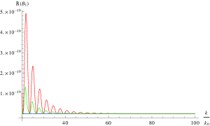
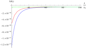
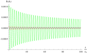
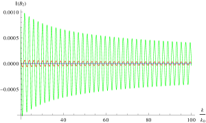
Bζ(B1B2)=(B1)(B2)+(B1)(B2),proportional-tosubscript𝐵𝜁subscript𝐵1subscript𝐵2subscript𝐵1subscript𝐵2subscript𝐵1subscript𝐵2\displaystyle B_{\zeta}\propto\Im(B_{1}B_{2})=\Re(B_{1})\Im(B_{2})+\Im(B_{1})\Re(B_{2})\,, (66)

where

B1subscript𝐵1\displaystyle B_{1} =\displaystyle= ζ(τe,k1)ζ(τe,k2)ζ(τe,k3),𝜁subscript𝜏𝑒subscript𝑘1𝜁subscript𝜏𝑒subscript𝑘2𝜁subscript𝜏𝑒subscript𝑘3\displaystyle\zeta(\tau_{e},k_{1})\zeta(\tau_{e},k_{2})\zeta(\tau_{e},k_{3})\,, (67)
B2subscript𝐵2\displaystyle B_{2} =\displaystyle= 2I1(k1,k2,k3)k12I2(k1,k2,k3)+ two permutations of k1,k2, and k3.2subscript𝐼1subscript𝑘1subscript𝑘2subscript𝑘3superscriptsubscript𝑘12subscript𝐼2subscript𝑘1subscript𝑘2subscript𝑘3 two permutations of subscript𝑘1subscript𝑘2 and subscript𝑘3\displaystyle 2I_{1}(k_{1},k_{2},k_{3})-k_{1}^{2}I_{2}(k_{1},k_{2},k_{3})+\mbox{ two permutations of }k_{1},k_{2},\mbox{ and }k_{3}\,. (68)

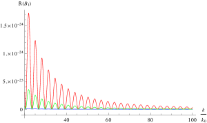
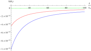
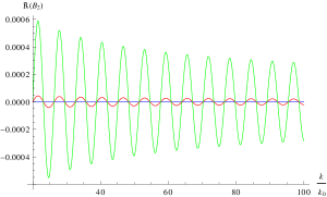
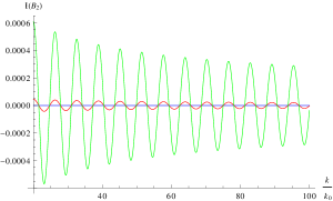
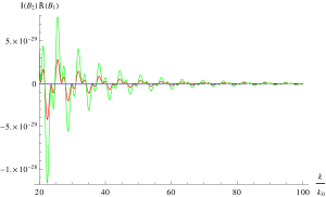
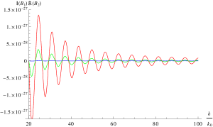
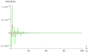
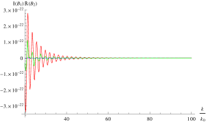
First of all we can see from fig. (17) and fig. (20) that the dominant contribution to the bispectrum comes from the term (B1)(B2)subscript𝐵1subscript𝐵2\Im(B_{1})\Re(B_{2}), which is in fact behaving in the same way as the bispectrum respect to the variaton of n𝑛n. Both the terms (B2)subscript𝐵2\Re(B_{2}) and (B1)subscript𝐵1\Im(B_{1}) are behaving like the spectrum, i.e., are larger for larger values of n𝑛n, but since (B1)subscript𝐵1\Im(B_{1}) is negative, their product (B1)(B2)subscript𝐵1subscript𝐵2\Im(B_{1})\Re(B_{2}), and consequently the bispectrum which is dominated by it, is behaving in the opposite way, i.e. is decreasing when n𝑛n in increasing. The effect is not noticeable in the case of n=2/3𝑛23n=2/3, because in this case (B2)subscript𝐵2\Re(B_{2}) is very closed to zero, while it is clear for n=3𝑛3n=3 and n=4𝑛4n=4.

Refer to caption
Refer to caption
Figure 17: The real part of B1subscript𝐵1B_{1} is plotted on the left, and the imaginary part on the right, for the small scales squeezed limit. The parameter λ𝜆\lambda is constant, λ=3.9×10¹⁹𝜆3.9superscript1019\lambda=3.9\times 10^{-19}, while n=2/3𝑛23n=2/3 (blue), n=3𝑛3n=3 (red), and n=4𝑛4n=4 (green).
Refer to caption
Refer to caption
Figure 18: The real part of B2subscript𝐵2B_{2} is plotted on the left, and the imaginary part on the right, for the small scales squeezed limit. The parameter λ𝜆\lambda is constant, λ=3.9×10¹⁹𝜆3.9superscript1019\lambda=3.9\times 10^{-19}, while n=2/3𝑛23n=2/3 (blue), n=3𝑛3n=3 (red), and n=4𝑛4n=4 (green).
Refer to caption
Refer to caption
Figure 19: The products (B1)(B2)subscript𝐵1subscript𝐵2\Re(B_{1})\Im(B_{2}) and (B1)(B2)subscript𝐵1subscript𝐵2\Im(B_{1})\Re(B_{2}) are plotted for the small scales squeezed limit. The parameter λ𝜆\lambda is constant, λ=3.9×10¹⁹𝜆3.9superscript1019\lambda=3.9\times 10^{-19}, while n=2/3𝑛23n=2/3 (blue), n=3𝑛3n=3 (red), and n=4𝑛4n=4 (green).
Refer to caption
Refer to caption
Figure 20: The real part of B1subscript𝐵1B_{1} is plotted on the left, and the imaginary part on the right, for the small scales equilateral limit. The parameter λ𝜆\lambda is constant, λ=3.9×10¹⁹𝜆3.9superscript1019\lambda=3.9\times 10^{-19}, while n=2/3𝑛23n=2/3 (blue), n=3𝑛3n=3 (red), and n=4𝑛4n=4 (green).
Refer to caption
Refer to caption
Figure 21: The real part of B2subscript𝐵2B_{2} is plotted on the left, and the imaginary part on the right, for the small scales equilateral limit. The parameter λ𝜆\lambda is constant, λ=3.9×10¹⁹𝜆3.9superscript1019\lambda=3.9\times 10^{-19}, while n=2/3𝑛23n=2/3 (blue), n=3𝑛3n=3 (red), and n=4𝑛4n=4 (green).
Refer to caption
Refer to caption
Figure 22: The products (B1)(B2)subscript𝐵1subscript𝐵2\Re(B_{1})\Im(B_{2}) and (B1)(B2)subscript𝐵1subscript𝐵2\Im(B_{1})\Re(B_{2}) are plotted for the small scales squeezed limit. The parameter λ𝜆\lambda is constant, λ=3.9×10¹⁹𝜆3.9superscript1019\lambda=3.9\times 10^{-19}, while n=2/3𝑛23n=2/3 (blue), n=3𝑛3n=3 (red), and n=4𝑛4n=4 (green).

XI Conclusions

We have studied the effects of a general type of features produced by discontinuities of the derivatives of the potential. We found that each different type of feature has distinctive effects on the spectrum and bispectrum of curvature perturbations which depend both on the order n𝑛n and on the amplitude λ𝜆\lambda of discontinuity. The spectrum of primordial curvature perturbations shows oscillations around the scale k0subscript𝑘0k_{0} which leaves the horizon at the time τ0subscript𝜏0\tau_{0} when the feature occurs, with amplitude and phase determined by the parameters n𝑛n and λ𝜆\lambda.

Both in the squeezed and equilateral small scale limit the bispectrum has an oscillatory behavior whose phase depends on the parameters determining the discontinuity, and whose amplitude is inversely proportional to the scale. The large scale bispectrum in the squeezed and equilateral limits have a very similar form and are linearly suppressed.
The analytical approximation for the spectrum is in good agreement with the numerical results, and improves substantially the accuracy for large scales respect to previous studies. The analytical approximations for the bispectrum are in good agreement with numerical calculations at large scales in both the squeeze and equilateral limit. At small scales we found an analytical template which is in very good agreement with the numerical calculations both in the squeezed and equilateral limit, and is able to account for both the oscillations and the amplitude of the bispectrum.

The type of feature we have studied generalize previous models such as the Starobinsky model or the mass step aer , providing a general framework to classify and model phenomenologically non Gaussian features in CMB observations or in large scale structure survey data. In the future it would be interesting to find the parameters which better fit different non Gaussian features in observational data and to investigate what more fundamental physical mechanism, such as phase transitions for example, could actually produce these features.

Acknowledgements.
AER work was supported by the Dedicacion exclusiva and Sostenibilidad programs at UDEA, the UDEA CODI projects IN10219CE and 2015-4044. This work was supported by the European Union (European Social Fund, ESF) and Greek national funds under the “ARISTEIA II” Action.

Appendix A

In this appendix we obtain analytical approximations for the integrals which are necessary for the calculation of small scale limit bispectrum

𝒜1(τ,k1,k2,k3,q)subscript𝒜1𝜏subscript𝑘1subscript𝑘2subscript𝑘3𝑞\displaystyle\mathcal{A}_{1}(\tau,k_{1},k_{2},k_{3},q) \displaystyle\equiv dτa(τ)qζ(τ,k1)ζ(τ,k2)ζ(τ,k3),\displaystyle\int d\tau\,a(\tau)^{q}\zeta^{*}(\tau,k_{1})\zeta^{\prime}{}^{*}(\tau,k_{2})\zeta^{\prime}{}^{*}(\tau,k_{3})\,, (69)
𝒜2(τ,k1,k2,k3,q)subscript𝒜2𝜏subscript𝑘1subscript𝑘2subscript𝑘3𝑞\displaystyle\mathcal{A}_{2}(\tau,k_{1},k_{2},k_{3},q) \displaystyle\equiv 𝑑τa(τ)qζ(τ,k1)ζ(τ,k2)ζ(τ,k3).differential-d𝜏𝑎superscript𝜏𝑞superscript𝜁𝜏subscript𝑘1superscript𝜁𝜏subscript𝑘2superscript𝜁𝜏subscript𝑘3\displaystyle\int d\tau\,a(\tau)^{q}\zeta^{*}(\tau,k_{1})\zeta^{*}(\tau,k_{2})\zeta^{*}(\tau,k_{3})\,. (70)

In order to simplify the calculation we fix ϵ(τ)=ϵ(τ0)italic-ϵ𝜏italic-ϵsubscript𝜏0\epsilon(\tau)=\epsilon(\tau_{0}) only in the analytical approximation for perturbations modes in eq. (39), while we keep ϵ(τ),η(τ)italic-ϵ𝜏𝜂𝜏\epsilon(\tau),\eta(\tau) as functions of conformal time when they appear explicitly in the integrand.

After some rather cumbersome calculation the final result can be written in this general form

𝒜i(τ,k1,k2,k3,q)=(1)i(k2k3)2(2i)H03q(4ϵ0k1k2k3)3/2×\displaystyle\mathcal{A}_{i}(\tau,k_{1},k_{2},k_{3},q)=\frac{(-1)^{i}(k_{2}k_{3})^{2(2-i)}H_{0}^{3-q}}{\left(4\epsilon_{0}k_{1}k_{2}k_{3}\right)^{3/2}}\times (71)
{αk1[\displaystyle\Biggl{\{}\alpha^{*}_{k_{1}}\biggl{[} αk2(i(τ,k1,k2,k3,q)αk3i(τ,k1,k2,k3,q)βk3)subscriptsuperscript𝛼subscript𝑘2subscript𝑖𝜏subscript𝑘1subscript𝑘2subscript𝑘3𝑞subscriptsuperscript𝛼subscript𝑘3subscript𝑖𝜏subscript𝑘1subscript𝑘2subscript𝑘3𝑞subscriptsuperscript𝛽subscript𝑘3\displaystyle\alpha^{*}_{k_{2}}\Bigl{(}\mathcal{B}_{i}(\tau,k_{1},k_{2},k_{3},q)\alpha^{*}_{k_{3}}-\mathcal{B}_{i}(\tau,k_{1},k_{2},-k_{3},q)\beta^{*}_{k_{3}}\Bigr{)}
+\displaystyle+ βk2(i(τ,k1,k2,k3,q)αk3+i(τ,k1,k2,k3,q)βk3)]\displaystyle\beta^{*}_{k_{2}}\Bigl{(}-\mathcal{B}_{i}(\tau,k_{1},-k_{2},k_{3},q)\alpha^{*}_{k_{3}}+\mathcal{B}_{i}(\tau,k_{1},-k_{2},-k_{3},q)\beta^{*}_{k_{3}}\Bigr{)}\biggr{]}
+βk1[\displaystyle+\beta^{*}_{k_{1}}\biggl{[} βk2(i(τ,k1,k2,k3,q)βk3i(τ,k1,k2,k3,q)αk3)subscriptsuperscript𝛽subscript𝑘2subscriptsuperscript𝑖𝜏subscript𝑘1subscript𝑘2subscript𝑘3𝑞subscriptsuperscript𝛽subscript𝑘3subscriptsuperscript𝑖𝜏subscript𝑘1subscript𝑘2subscript𝑘3𝑞subscriptsuperscript𝛼subscript𝑘3\displaystyle\beta^{*}_{k_{2}}\Bigl{(}\mathcal{B}^{*}_{i}(\tau,k_{1},k_{2},k_{3},q)\beta^{*}_{k_{3}}-\mathcal{B}^{*}_{i}(\tau,k_{1},k_{2},-k_{3},q)\alpha^{*}_{k_{3}}\Bigr{)}
+\displaystyle+ αk2(i(τ,k1,k2,k3,q)βk3+i(τ,k1,k2,k3,q)αk3)]},\displaystyle\alpha^{*}_{k_{2}}\Bigl{(}-\mathcal{B}^{*}_{i}(\tau,k_{1},-k_{2},k_{3},q)\beta^{*}_{k_{3}}+\mathcal{B}^{*}_{i}(\tau,k_{1},-k_{2},-k_{3},q)\alpha^{*}_{k_{3}}\Bigr{)}\biggr{]}\Biggr{\}},

where

1=(ikT)q4(kTΓ(3q,iτkT)+k1Γ(4q,iτkT)),subscript1superscriptisubscript𝑘𝑇𝑞4subscript𝑘𝑇Γ3𝑞i𝜏subscript𝑘𝑇subscript𝑘1Γ4𝑞i𝜏subscript𝑘𝑇\displaystyle\mathcal{B}_{1}=(\mathrm{i}k_{T})^{q-4}\Bigl{(}k_{T}\Gamma(3-q,-\mathrm{i}\tau k_{T})+k_{1}\Gamma(4-q,-\mathrm{i}\tau k_{T})\Bigr{)}\,, (72)
2=(ikT)q4[kT3(Γ(1q,iτkT)+Γ(2q,iτkT))\displaystyle\mathcal{B}_{2}=(\mathrm{i}k_{T})^{q-4}\Bigl{[}k_{T}^{3}\Bigl{(}\Gamma(1-q,-\mathrm{i}\tau k_{T})+\Gamma(2-q,-\mathrm{i}\tau k_{T})\Bigr{)}
+kTij3kikjΓ(3q,iτkT)+k1Γ(4q,iτkT)],\displaystyle+k_{T}\sum_{i\neq j}^{3}k_{i}k_{j}\Gamma(3-q,-\mathrm{i}\tau k_{T})+k_{1}\Gamma(4-q,-\mathrm{i}\tau k_{T})\Bigr{]}\,, (73)
kT=k1+k2+k3,subscript𝑘𝑇subscript𝑘1subscript𝑘2subscript𝑘3\displaystyle k_{T}=k_{1}+k_{2}+k_{3}\,,

and the ΓΓ\Gamma denotes the incomplete gamma functions defined by

Γ(r,x)=xtr1et𝑑t.Γ𝑟𝑥superscriptsubscript𝑥superscript𝑡𝑟1superscript𝑒𝑡differential-d𝑡\displaystyle\Gamma(r,x)=\int_{x}^{\infty}t^{r-1}e^{-t}dt\,. (74)

References

  • (1) E. Komatsu et al., (2009), arXiv:0902.4759.
  • (2) WMAP, G. Hinshaw et al., Astrophys.J.Suppl. 208, 19 (2013), arXiv:1212.5226.
  • (3) Planck Collaboration, P. Ade et al., (2013), arXiv:1303.5076.
  • (4) K. N. Abazajian et al., ArXiv e-prints (2013), arXiv:1309.5381.
  • (5) C. Reichardt et al., Astrophys.J. 755, 70 (2012), arXiv:1111.0932.
  • (6) J. L. Sievers et al., (2013), arXiv:1301.0824.
  • (7) WMAP, C. Bennett et al., Astrophys.J.Suppl. 208, 20 (2013), arXiv:1212.5225.
  • (8) Planck Collaboration, P. Ade et al., (2013), arXiv:1303.5082.
  • (9) X. Chen, Adv.Astron. 2010, 638979 (2010), arXiv:1002.1416.
  • (10) A. A. Starobinsky, Phys.Lett. B91, 99 (1980).
  • (11) Planck Collaboration, P. Ade et al., (2013), arXiv:1303.5084.
  • (12) J. Martin, L. Sriramkumar, and D. K. Hazra, ArXiv e-prints (2014), arXiv:1404.6093.
  • (13) S. Dorn, E. Ramirez, K. E. Kunze, S. Hofmann, and T. A. Ensslin, JCAP 1406, 048 (2014), arXiv:1403.5067.
  • (14) D. K. Hazra, L. Sriramkumar, and J. Martin, JCAP5, 26 (2013), arXiv:1201.0926.
  • (15) V. Sreenath, R. Tibrewala, and L. Sriramkumar, JCAP12, 37 (2013), arXiv:1309.7169.
  • (16) A. A. Starobinsky, JETP Lett. 55, 489 (1992).
  • (17) J. Hamann, L. Covi, A. Melchiorri, and A. Slosar, Phys.Rev. D76, 023503 (2007), arXiv:astro-ph/0701380.
  • (18) D. K. Hazra, M. Aich, R. K. Jain, L. Sriramkumar, and T. Souradeep, JCAP 1010, 008 (2010), arXiv:1005.2175.
  • (19) A. A. Starobinsky, Grav.Cosmol. 4, 88 (1998), arXiv:astro-ph/9811360.
  • (20) M. Joy, V. Sahni, and A. A. Starobinsky, Phys.Rev. D77, 023514 (2008), arXiv:0711.1585.
  • (21) M. Joy, A. Shafieloo, V. Sahni, and A. A. Starobinsky, JCAP 0906, 028 (2009), arXiv:0807.3334.
  • (22) M. J. Mortonson, C. Dvorkin, H. V. Peiris, and W. Hu, Phys.Rev. D79, 103519 (2009), arXiv:0903.4920.
  • (23) F. Arroja, A. E. Romano, and M. Sasaki, Phys.Rev. D84, 123503 (2011), arXiv:1106.5384.
  • (24) A. E. Romano and M. Sasaki, Phys.Rev. D78, 103522 (2008), arXiv:0809.5142.
  • (25) J. A. Adams, G. G. Ross, and S. Sarkar, Nucl.Phys. B503, 405 (1997), arXiv:hep-ph/9704286.
  • (26) S. Gariazzo, C. Giunti, and M. Laveder, JCAP 1504, 023 (2015), arXiv:1412.7405.
  • (27) D. Langlois, Lect.Notes Phys. 800, 1 (2010), arXiv:1001.5259.
  • (28) A. R. Liddle and D. Lyth, (2000).
  • (29) D. K. Hazra, A. Shafieloo, G. F. Smoot, and A. A. Starobinsky, Phys.Rev.Lett. 113, 071301 (2014), arXiv:1404.0360.
  • (30) R. Bousso, D. Harlow, and L. Senatore, Phys. Rev. D91, 083527 (2015), arXiv:1309.4060.
  • (31) J. M. Maldacena, JHEP 0305, 013 (2003), arXiv:astro-ph/0210603.
  • (32) H. Collins, (2011), arXiv:1101.1308.
  • (33) T. Bunch and P. Davies, Proc.Roy.Soc.Lond. A360, 117 (1978).
  • (34) X. Chen, R. Easther, and E. A. Lim, JCAP 0706, 023 (2007), arXiv:astro-ph/0611645.
  • (35) S. Weinberg, Phys.Rev. D72, 043514 (2005), arXiv:hep-th/0506236.
  • (36) P. Adshead, C. Dvorkin, W. Hu, and E. A. Lim, Phys.Rev. D85, 023531 (2012), arXiv:1110.3050.
  • (37) X. Chen, R. Easther, and E. A. Lim, JCAP 0804, 010 (2008), arXiv:0801.3295.