Active Clinical Trials for Personalized Medicine

Abstract

Individualized treatment rules (ITRs) tailor treatments according to individual patient characteristics. They can significantly improve patient care and are thus becoming increasingly popular. The data collected during randomized clinical trials are often used to estimate the optimal ITRs. However, these trials are generally expensive to run, and, moreover, they are not designed to efficiently estimate ITRs. In this paper, we propose a cost-effective estimation method from an active learning perspective. In particular, our method recruits only the “most informative” patients (in terms of learning the optimal ITRs) from an ongoing clinical trial. Simulation studies and real-data examples show that our active clinical trial method significantly improves on competing methods. We derive risk bounds and show that they support these observed empirical advantages.

Key words: Active Learning, Clinical Trial, Individualized Treatment Rule, Personalized Medicine, Risk Bound.

1 Introduction

It is widely recognized that different patients respond differently to the same treatment. Recent advances in personalized medicine have the potential to improve treatment decisions in clinical practice by tailoring the clinical interventions to the patient characteristics. These characteristics include demographics, medical histories, and genetic or genomic information (Hamburg and Collins, 2010). It is anticipated that these new developments in personalized medicine may salvage some failed medications, which is especially important given the low overall success rate recently observed in clinical trials (DiMasi et al., 2010).

The success of personalized medicine is contingent on the correct identification of the best treatments for each individual. One research direction is subgroup analysis, where the patients are grouped based on the estimated individual-level treatment differences (Cai et al., 2011; Foster et al., 2011). Alternatively, vigorous research has focused on finding optimal treatment regimens, which yield the greatest benefit overall for the whole population. Some methods involve fitting a regression model for the response, and recommending the treatment achieving the best prediction (Qian and Murphy, 2011). Instead, Zhao et al. (2012) explore the optimal individualized therapies from a classification perspective (see also Zhang et al. (2012)). All these methods are implemented using data from randomized clinical trials (RCTs). However, traditional RCTs are primarily designed to confirm the efficacy of new treatments; they do not generate comprehensive personalized therapy rules in an efficient manner. Consequently, post-mining data from RCTs is not ideal for finding optimal treatment strategies (Cui et al., 2002; Lagakos, 2006). RCTs generally require a large sample size to demonstrate the efficacy of a candidate treatment, and they can be expensive to run because of the need to treat and monitor a large number of subjects. In addition, RCTs waste trial resources on subjects who experience treatment effects that are relatively large. Therefore, it would be desirable to design cost-effective clinical trials for personalized medicine. Such trials would highlight individual differences in responses and take advantage of continuing advances revealed in the trial (Singer, 2005).

We propose an active learning framework for conducting clinical trials, called active clinical trials. In these trials, patients are judiciously recruited so that the optimal ITRs can be learned with fewer patients being randomized; this is a cost-effective method. Unlike traditional RCTs, we will exclude the patients for whom the benefit from one of the treatments is clearly observed, thus concentrating on those for whom the difference is less pronounced. Specifically, within the classification framework (Zhao et al., 2012), we first construct “confidence intervals” for the optimal decision boundary using the data accumulated so far based on either a frequentist or Bayesian approach. We then selectively enroll the patients whose optimal treatments are hard to determine, i.e., their benefit differences from the different treatments are “small,” based on the above confidence intervals. Those patients are viewed as the most informative for the purpose of learning the optimal ITRs, and thus they are recruited for randomizations at the next stage. As will be seen in the empirical and theoretical analysis, the real-time selection of the right patients indeed improves the chance of discovering optimal ITRs with a drastically reduced sample size and cost.

Our work is related to the topic of budgeted learning (Madani et al., 2004; Raghavan et al., 2006; Deng et al., 2007) in computer science. These work aim to find the most accurate classifier subject to a fixed budget. The main difference is that the responses for the subjects are assumed to be known, and the covariate information is required. Our work in the clinical trial setting sequentially applies treatments to selected subjects and then observes their responses. Another related topic in computer science is the “multi-armed bandit problem” (Robbins, 1952), where resources are allocated among multiple arms given a fixed budget. One tries to maximize the cumulative rewards over all allocations. This perspective is also taken in response-adaptive trials (Rosenberger and Lachin, 1993; Hu and Rosenberger, 2006), which allocate more patients to the better treatment based on the available patient responses. Thus, such trials can be viewed as exploitative, since most of them adopt myopic strategies by exploiting the current best arm. Our method is more exploratory, exploring patients close to the decision boundary to learn better individualized treatment rules for future practice. Some adaptive enrichment designs (Wang et al., 2009; Simon and Simon, 2013) are similar in that they allow the eligibility criteria to be updated during the trial. However, our primary goal is to construct informative and favorable ITRs rather than to confirm the efficacy of one treatment over another. Our method is also different from adaptive randomization procedures, which primarily aim to place more subjects onto the treatment arm that is more promising (Rosenberger et al., 2012). Deng et al. (2011b) proposed a minimax bandit model for clinical trials that carefully distributes the trial resources, with the same objective as our method. However, they specify subpopulations in advance, and the optimal treatments are learned for each subpopulation. The resulting ITRs may not be ideal if the subpopulations are not formed correctly.

In Section 2, we introduce a general methodology for conducting active clinical trials, along with methods for constructing optimal ITRs using the accumulated data. In Section 3, we discuss the theoretical properties of our approach by providing a finite sample upper bound on the difference in the expected outcome under the estimated ITR and the optimal ITR. In Section 4, we conduct extensive simulation studies to examine the empirical performance and also compare the results with those of Deng et al. (2011b). Two real data examples are presented in Section 5, and Section 7 provides a discussion. The technical details are presented in the Appendix and the Supplementary Materials.

2 Methodology

2.1 Optimal Individual Treatment Rule

In this section, we discuss a probabilistic framework for studying the optimal ITRs that is similar to that of Qian and Murphy (2011) and Zhao et al. (2012). Let $({X},A,R)$ be a random triple with a joint distribution $P$. Here, ${X}\in\mathbb{R}^{p}$ denotes the patient’s baseline covariates with marginal distribution $\Pi$, $A$ is a binary treatment assignment taking values in $\{-1,1\}$, and $R$ stands for the treatment outcome (a larger value of $R$ corresponds to a better outcome). An ITR $D(\cdot)$ is defined as a function from the covariate space $\mathbb{R}^{p}$ into the treatment space $\{-1,1\}$.

We use the value function, denoted as $V(D)$, to measure the quality of $D$, which is a marginal mean outcome representing the overall population mean were all patients to receive treatment according to $D$. Our goal is to identify the optimal ITR that yields the maximum $V(D)$. For any ITR $D$, let $P^{D}$ be the distribution of $({X},A,R)$ when $A=D({X})$, and let $\mathbb{E}^{D}$ be the corresponding expectation. The value function $V(D)=\mathbb{E}^{D}(R)$. Qian and Murphy (2011) show that $V(D)$ can be expressed as

$$V(D)=\mathbb{E}\left[\frac{RI(A=D({X}))}{\pi(A;{X})}\right],$$ (2.1)

where $\mathbb{E}$ denotes the expectation w.r.t. the joint distribution $P$, $I(\cdot)$ is an indicator function, and $\pi(a;{X})$ is the conditional probability $P(A=a|{X})$ for $a\in\{-1,1\}$. For simplicity, we assume a pure randomization scheme with equal probability for different assignments, i.e., $\pi(a;{X})=1/2$, throughout the paper.

Let $D^{*}$ denote the optimal treatment rule that maximizes $V({D})$. By rewriting $V(D)$ as $V(D)=\mathbb{E}\Big{(}\mathbb{E}[RI(D(X)=1)|A=1,X]+\mathbb{E}[RI(D(X)=-1)|A=-1,X]\Big{)}$, we obtain

$$D^{*}({x})=\mbox{sign}\{f^{*}(x)\},$$ (2.2)

where $f^{*}(x):=\mathbb{E}[R|A=1,{X}={x}]-\mathbb{E}[R|A=-1,{X}={x}]$ is called the contrast function. The optimal decision boundary is just the level set $\{{x}\in\mathbb{R}^{p}:f^{*}({x})=0\}$. As can be seen, the overall benefit will be maximized if the patients satisfying $f^{*}(x)\geq 0$ receive the alternative treatment (treatment 1), and the others receive standard care (treatment -1). Hence, the decision is tailored according to the patient’s characteristics represented by $X$.

To estimate the optimal ITR $D^{*}$ from the data $\{X^{(i)},A^{(i)},R^{(i)}\}_{i=1}^{n}$, usually collected from a clinical trial, one can fit a parametric or nonparametric regression model for $\mathbb{E}[R|A=a,{X}=x]$ (equivalently, $f^{\ast}(x)$), and then estimate the optimal ITR by plugging the fitted model into (2.2). Alternatively, we can replace the problem of maximizing (2.1) by minimizing a weighted classification error $\mathbb{E}\left[{RI(A\neq{D}({X}))}/{\pi(A;{X})}\right]$. In this case, existing classification techniques, e.g., support vector machines, can be adapted to estimate $D^{*}({x})$; see Zhao et al. (2012) for more details. All of the above methods take the whole (randomized) clinical trial data as an input, and thus they have no influence on the data collection process. They belong to the class of passive learning methods, also called batch learning. In clinical trials, the patient recruiting process is usually long, and the treatment and monitoring process can be extremely expensive. With a limited budget and a fixed sample size, we should wisely allocate the resources, i.e., decide who to recruit, in order to learn the optimal ITRs at a lower cost. This motivates us to propose active clinical trials that can identify the optimal ITRs with a significantly reduced cost.

2.2 Active Clinical Trials

The active learning (AL) approach in the classification literature is shown to produce accurate classifiers with a significantly reduced number of label requests; see Balcan et al. (2008), Dasgupta et al. (2007), Castro and Nowak (2008), Koltchinskii (2010), Hanneke (2011), and Minsker (2012). Recall that the estimation of ITRs can be thought of as a classification problem. For example, a patient with a small outcome given the assigned treatment is potentially misclassified. We use AL techniques to select the “most informative” patients based on a given pool of prognostic variables, and then we randomize only the patients with these “informative” characteristics. The intuition behind this patient-selection process is simple: if we have confidence that certain patients will benefit from a particular treatment, we should not recruit them into the study since they are not likely to contribute to the estimation of ITRs. However, it is hard to determine the optimal treatment, i.e., the sign of $f^{*}(x)$, for the patients whose baseline variables are “close” to the optimal decision boundary. As will be seen from the empirical and theoretical analysis, patients with such features are more “informative” in the sense that their outcomes after randomization provide more insight into the optimal ITRs (to be applied to future patients). Moreover, since patients will not be randomized if we have confidence in the treatment they should receive, they are less likely to be exposed to ineffective medications.

We assume that there is no delay in observing the outcome. For $S\subset\mbox{supp}(\Pi)$ and a function $f:\mathbb{R}^{p}\mapsto\mathbb{R}$, let $f|_{S}:S\mapsto\mathbb{R}$ be the restriction of $f$ onto $S$, and define $\|f\|_{\infty,S}=\left\|f|_{S}\right\|_{\infty}:=\sup\limits_{x\in S}|f(x)|$. Given $\delta>0$, set

$$\mathcal{F}_{\infty,S}(f,\delta):=\{g:S\mapsto\mathbb{R}:\ \|g-f\|_{\infty,S}\leq\delta\}$$

as a $\delta$-band around $f$ on $S$. A precise description is given in Algorithm 1. Here, we introduce the important notion of an active set (Minsker, 2012), which underlies the majority of active learning algorithms. At step $k$ of our Algorithm 1, the active set $AS_{k}$ is defined to be the set of baseline variables for which the best treatment is not yet known. The active set is characterized by the confidence interval, i.e., $x$ belongs to the active set if and only if the confidence interval for $f^{\ast}(x)$ contains both positive and negative elements; Figures 2 and 2 below illustrate this. The approximation of $AS_{k}$ using a regular set ${\rm act}_{k}$ is discussed in Appendix A.1.

input : Sample size limit $N$; confidence $\alpha$

output : $\widehat{D}:=\mbox{sign}(\widehat{f})$

1 $k=0$, ${\rm act}_{0}:=\mbox{supp}(\Pi)$;

Set the initial $N_{0}:=2\lfloor\sqrt{N}\rfloor$, and $LB:=N-N_{0}$;

for $i=1$ to $N_{0}$ do

       Recruit $X^{(i,0)}$ from $\Pi$;

       Randomize $X^{(i,0)}$ to treatment $A^{(i,0)}=1$ or $-1$ with equal probability;

       Observe $R^{(i,0)}$;

      

end for

2Construct the estimator $\widehat{f}_{0}(x)$ of $f^{*}$ from $S_{0}=\left\{\left(X^{(i,0)},A^{(i,0)},R^{(i,0)}\right)\right\}_{i=1}^{N_{0}}$;

while $LB>0$ do

      3 $\widehat{\mathcal{F}}_{k}:=\left\{f\ :\ f|_{{{\rm act}}_{k}}\in\mathcal{F}_{\infty,{\rm act}_{k}}(\widehat{f}_{k};\frac{3}{2}\delta_{k}),\ \ f|_{\mbox{supp}(\Pi)\setminus{\rm act}_{k}}\equiv\widehat{f}_{k-1}|_{\mbox{supp}(\Pi)\setminus{\rm act}_{k}}\right\}$ /* $\delta_{k}$: confidence band size */;

      4 $k:=k+1$;

       $AS_{k}:=\left\{x\in\mbox{supp}(\Pi):\ \exists f_{1},f_{2}\in\widehat{\mathcal{F}}_{k-1},\mbox{sign}(f_{1}(x))\neq\mbox{sign}(f_{2}(x))\right\}$ /* active set */;

       Approximate $AS_{k}$ with a regular set ${\rm act}_{k}$;

      5 if ${\rm act}_{k}\cap\mbox{supp}(\Pi)=\emptyset$ then

            break

       end if

      else

             $N_{k}=2N_{k-1}$;

             for $i=1$ to $\lfloor N_{k}\cdot\Pi({\rm act}_{k})\rfloor$ do

                   Recruit $X^{(i,k)}$ from the active set $\widehat{\Pi}_{k}:=\Pi_{{\rm act}_{k}}(dx)$;

                   Randomize $X^{(i,k)}$ to treatment $A^{(i,k)}=1$ or $-1$ with equal probability;

                   Observe $R^{(i,k)}$, $S_{k}:=\left\{\left(X^{(i,k)},A^{(i,k)},R^{(i,k)}\right),\ i\leq\lfloor N_{k}\cdot\Pi({\rm act}_{k})\rfloor\right\}$;

                  

             end for

            Construct the estimator $\widehat{f}_{k}(\cdot)$ of $f^{*}$ based on $S_{k}$;

             $LB:=LB-\lfloor N_{k}\cdot\Pi({\rm act}_{k})\rfloor$;

             $\widehat{f}:=\widehat{f}_{k}$ /* keeping track of the most recent estimator */;

            

       end if

      

end while

Algorithm 1 Active Clinical Trials for Personalized Medicine

Figure 1: Confidence band for the contrast function.

Figure 2: $X^{(1)}$ belongs to the active set; $X^{(2)}$ does not.

In practice, it is not necessary to evaluate the active sets explicitly at each step. Instead, at step $k$, we repeat the following two steps until we reach the number of patients that can be randomized:

1. Recruit a group of new patients with baseline variables ${X}^{(i,k)},i=1,\ldots,N_{k}$.

2. Let $\widehat{f}_{i,k}(X^{(i,k)})$ be the estimator of $f^{\ast}(X^{(i,k)})$ based on $S_{k}$ and $I_{i,k}=[\widehat{f}_{k}(X^{(i,k)})-\delta(X^{(i,k)}),\widehat{f}_{k}(X^{(i,k)})+\delta(X^{(i,k)})]$ be the confidence interval, where $S_{k}$ is defined in Algorithm 1 and represents the available sample in the $k^{th}$ step.

   1. If $0\notin I_{i,k}$: drop the patient from the study.

   2. If $0\in I_{i,k}$: randomize the patient, record the outcome $R$, and add $(X^{(i,k)},A^{(i,k)},R^{(i,k)})$ to the current sample.

The above procedure gives a data set containing “the most informative” observations for predicting the optimal treatment. For every new patient, this data set will be used to predict the treatment rule based on that individual’s baseline variables. At each iteration, we must specify an estimator of the contrast function and the corresponding confidence interval. In the next section, we will propose two construction methods based on kernel estimation and Gaussian process regression, respectively. We remark that the empirical performance of our method is essentially controlled by the confidence level that we set. This level also determines the rejection ratio, e.g., $N=100$ out of 140 total iterations in simulation Scenario 1 of Section 4.

2.3 Confidence Interval Construction

2.3.1 Kernel Smoothing Approach

Let $K$ be a smooth kernel function (with bandwidth $h_{n}$) satisfying Assumption (A2) in Section 3. Define $K_{h_{n}}({x}_{0}-{X}):=K(({x}_{0}-{X})/h_{n})/h_{n}^{p}$. Let $\eta_{j}(x):=\mathbb{E}[R|A=j,X=x],j=\pm 1,$ be the conditional expectation of $R$ given $A$ and $X$. Given $n$ observations from $P$, we propose the estimators $\widehat{\eta}_{j}(\cdot;h_{n})$ for $j=\pm 1$, and the plug-in estimator $\widehat{f}(\cdot;h_{n})$ of the contrast function $f^{\ast}(\cdot)$. At any fixed point ${x}_{0}$,

$$\widehat{\eta}_{j}(x_{0};h_{n})=\frac{\sum\limits_{i=1}^{n}K_{h_{n}}({x}_{0}-{X}^{(i)})I(A^{(i)}=j)R^{(i)}}{\sum\limits_{i=1}^{n}K_{h_{n}}({x}_{0}-{X}^{(i)})I(A^{(i)}=j)},\ j=\pm 1,$$ (2.3)

$$\widehat{f}({x}_{0};h_{n})=\widehat{\eta}_{1}(x_{0};h_{n})-\widehat{\eta}_{-1}(x_{0};h_{n}).$$

Here, $h_{n}=h_{n}({x}_{0})$ is an adaptive bandwidth parameter varying with ${x}_{0}$. We need to choose a proper $h_{n}({x}_{0})$, which controls the local amount of data near ${x}_{0}$, to optimally balance the estimation bias and variance; see Appendix A.2.2 for the technical details.

Assuming that both $\eta_{1}$ and $\eta_{-1}$ are Lipschitz continuous with Lipschitz constants bounded by $L$, we define

$$h_{n,j}(x_{0})=\inf\left\{h>0:\ L^{2}h^{2}\geq\frac{C_{1}(K,P)}{\sum\limits_{i=1}^{n}I\left\{\|x_{0}-X^{(i)}\|_{2}\leq h\right\}I\{A^{(i)}=j\}}\right\},\ j=\pm 1,$$

where $C_{1}(K,P)$ is a constant depending on the kernel $K$ and distribution $P$, and $\|\cdot\|_{2}$ is the usual Euclidean norm. Set

$$h_{n}(x_{0}):=\max\left(h_{n,1}(x_{0}),h_{n,-1}(x_{0})\right).$$ (2.4)

This choice mimics the usual “bias-variance tradeoff”: indeed, the bias of $\widehat{\eta}_{j}(x_{0};h)$ is bounded by the order of $Lh$, while $\Big{(}\sum\limits_{i=1}^{n}I\left\{\|x_{0}-X^{(i)}\|_{2}\leq h\right\}I\{A^{(i)}=j\}\Big{)}^{-1}$ plays the role of the variance parameter. Based on the above choice of $h_{n}({x}_{0})$, i.e., (2.4), we define the radius of the confidence interval to be

$$\delta({x}_{0}):=t\cdot Lh_{n}({x}_{0}),$$

where $t$ controls the coverage probability. The display above depends on the unknown constants $C_{1}(K,P)$ that must be chosen before running the algorithm. Given a certain confidence level, we recommend selecting the “confidence parameter” $t$ by reverting the coverage probability error that decays exponentially fast with $t$; see Corollary A.1.

Remark 1. We are aware that the proposed kernel methods are unfortunately affected by the “curse of dimensionality.” However, our theoretical analysis reveals that the empirical performance of our kernel estimate essentially depends on the “intrinsic dimension” $d$ of the support of the marginal distribution $\Pi$ (see Assumption (A3) in Section 3), which might be much lower than the ambient dimension $p$. The concept of the intrinsic dimension originated in geometry and was later introduced to statistics, e.g., Allard et al. (2012). It characterizes a low-dimensional representation embedded in a high-dimensional space. For example, when the data are linear, we may use principal component analysis to identify the subspace that contains the data. The number of important components is the intrinsic dimension $d$, which can be significantly smaller than the total number of covariates $p$. In practice, we follow the local singular value decomposition method, suggested in Little et al. (2009), to determine the intrinsic dimension.

2.3.2 Gaussian Process Regression Approach

The new method presented in this section is particularly well suited for applications since it is completely data-driven and does not require us to specify any unknown parameters in advance; its performance is demonstrated in Section 4. However, the price is that we must assume that the conditional distribution of the outcome $R$ given $(A,X)$ is Gaussian. In other words, if an individual with baseline variables $X$ receives treatment $A=j$, we assume that the outcome satisfies $R=\eta_{j}({X})+\varepsilon$ for $j=\pm 1$, where $\varepsilon\sim N(0,\sigma^{2})$. In this situation, we take a Bayesian approach by imposing a Gaussian process prior (defined by the mean $m(\cdot)$ and covariance $k(\cdot,\cdot)$) on functions $\eta_{1}(\cdot)$ and $\eta_{-1}(\cdot)$; see Chapter 2 of Rasmussen and Williams (2006). For simplicity, the mean function $m(\cdot)$ is set to be identically zero throughout this paper.

As before, the confidence interval of the contrast function builds upon those of $\eta_{1}(\cdot)$ and $\eta_{-1}(\cdot)$. Hence, we start from the inference procedure for $\eta_{1}(\cdot)$. Let $\{(X^{(i)},R^{(i)})\}_{i=1}^{n_{1}}$ be the observations corresponding to the individuals who received treatment $1$. The covariance function of the Gaussian process prior is set as a slight variant of the squared exponential kernel: given $x=(x_{1},\ldots,x_{p})$ and $x^{\prime}=(x^{\prime}_{1},\ldots,x^{\prime}_{p})\in\mathbb{R}^{p}$,

$$k_{\gamma}(x,x^{\prime})=\gamma_{0}\exp\left(-\sum_{l=1}^{p}\frac{(x_{l}-x^{\prime}_{l})^{2}}{2\gamma_{l}^{2}}\right)$$

for some positive $\gamma_{0},\ldots,\gamma_{p}$. Let $K_{\gamma}$ be a $p\times p$ matrix with entries $(K_{\gamma})_{l_{1},l_{2}}=k_{\gamma}(X_{l_{1}},X_{l_{2}})$, $l_{1},l_{2}=1,\ldots,p$. Under the Gaussian error assumption, the marginal distribution of the vector $\textbf{R}=(R^{(1)},\ldots,R^{(n_{1})})^{T}$ given $\textbf{X}=(X^{(1)},\ldots,X^{(n_{1})})$ is a multivariate Gaussian with mean $0$ and covariance matrix $K_{\textbf{R}}:=K_{\gamma}+\sigma^{2}I_{p},$ where $I_{p}$ is a $p\times p$ identity matrix. The “optimal” value $\Gamma_{\ast}:=(\gamma_{0}^{\ast},\ldots,\gamma_{p}^{\ast},\sigma_{\ast}^{2})$ of the parameter $\Gamma=(\gamma_{0},\ldots,\gamma_{p},\sigma^{2})$ is then “learned” from the data by finding a local maximum of the marginal log-likelihood

$$\log p(\textbf{R}|\textbf{X},\Gamma):=-\frac{1}{2}\textbf{R}^{T}K_{\textbf{R}}^{-1}\textbf{R}-\frac{1}{2}\log\det K_{\textbf{R}}-\frac{n_{1}}{2}\log 2\pi$$

with respect to $(\gamma_{0},\ldots,\gamma_{p},\sigma^{2})$; see Section 5.4.1 in Rasmussen and Williams (2006) for more details. Therefore, the Gaussian process regression is a global method that can automatically select the bandwidth by maximizing the data likelihood. This is in contrast with the previous kernel method where the bandwidth is selected locally; see Equation (2.4) above.

We next construct the confidence interval based on the posterior distribution of $\eta_{1}(\cdot)$ with the optimal $\Gamma_{\ast}$. Given a new observation with the baseline variable $x_{0}$, the value of $\eta_{1}(x_{0})$ is estimated by the posterior mean, denoted $\widehat{\eta}_{1}(x_{0})$, i.e.,

$$\widehat{\eta}_{1}(x_{0}):=k_{\Gamma_{\ast}}(x_{0},\textbf{X})\,K_{\textbf{R}}^{-1}\textbf{R},$$

where $k_{\Gamma_{\ast}}(x,x^{\prime}):=\gamma_{0}^{\ast}\exp(-\sum\limits_{l=1}^{p}{(x_{l}-x^{\prime}_{l})^{2}}/{2(\gamma^{\ast}_{l})^{2}})$ for $x,x^{\prime}\in\mathbb{R}^{p}$, and

$$k_{\Gamma_{\ast}}(x_{0},\textbf{X})=(k_{\Gamma_{\ast}}(x_{0},X^{(1)}),\ldots,k_{\Gamma_{\ast}}(x_{0},X^{(n_{1})})).$$

The variance of the posterior distribution is given by

$$\widehat{\sigma}_{1}^{2}(x_{0}):=k_{\Gamma_{\ast}}(x_{0},x_{0})-k_{\Gamma_{\ast}}(x_{0},\textbf{X})\,K_{\textbf{R}}^{-1}\,k_{\Gamma_{\ast}}(x_{0},\textbf{X})^{T}.$$

The square root of the posterior variance naturally controls the length of the confidence interval for $\eta_{1}(x_{0})$. For example, setting $\delta_{1}(x_{0}):=3\widehat{\sigma_{1}}(x_{0})$ gives the confidence interval for $\eta_{1}(x_{0})$ of posterior probability $>99\%$ (note that this may not correspond to the frequentist coverage).

Define $\widehat{\eta}_{-1}(x_{0})$ and the associated $\delta_{-1}(x_{0})$ analogously. We thus obtain a confidence interval with the center $\widehat{f}(x_{0}):=\widehat{\eta}_{1}(x_{0})-\widehat{\eta}_{-1}(x_{0})$ and the radius $\delta(x_{0}):=\delta_{1}(x_{0})+\delta_{-1}(x_{0})$. The numerical implementation of this Bayesian inference procedure can easily be performed with the gpml Matlab toolbox (Rasmussen and Nickisch, 2010).

3 Theoretical Analysis

In this section, we focus our theoretical analysis on the kernel smoothing approach. The frequentist property of the credible set for the nonparametric Bayesian method has not been well developed. Hence, a theoretical analysis of the Gaussian process regression method is beyond the scope of this paper.

For simplicity, we suppose that the marginal distribution $\Pi$ of the baseline variable vector $X$ is known. Note that Algorithm 1 does not need to know or estimate $\Pi$ explicitly, and this assumption is only for the theoretical analysis. In addition, we assume the following conditions on the kernel $K:\mathbb{R}^{p}\mapsto\mathbb{R}$ and the distribution $\Pi$:

(A0)

Both $\eta_{1}(x):=\mathbb{E}[R|A=1,{X}=x]$ and $\eta_{-1}(x):=\mathbb{E}[R|A=-1,{X}=x]$ are Lipschitz continuous on $\mathbb{R}^{p}$ with Lipschitz constants bounded by $L$.

(A1)

The random variable $|R|$ is bounded by $0<M<\infty$ a.s.

(A2)

$K(x)$ is a nonnegative, compactly supported, Lipschitz-continuous function with a Lipschitz constant $L_{K}$. Moreover, $K(x)\geq\ell_{K}I\{\|x\|_{2}\leq 1\}$ for some $\ell_{K}>0$.

(A3)

The “intrinsic dimension” of $\mbox{supp}(\Pi)$ is equal to $d$ for some integer $d\leq p$, and $\Pi$ is equivalent to the uniform distribution over its support; see Appendix A.1 for a more precise statement.

(A4)

Margin condition: there exist $K_{2}=K_{2}(\Pi),\gamma=\gamma(\Pi)>0$ such that for all $t>0$

$$\Pi\left(x:\ |f^{*}(x)|\leq t\right)\leq K_{2}t^{\gamma}.$$

Assumption (A3) says that over a “nice” set, $\Pi$ is close to the uniform distribution; see condition (A.1) in the Appendix. The intrinsic dimension $d$ is crucial here: in many applications, $p$ is large but $d$ is small (see Remark 1). Note that the rate in our main result, Theorem 3.1, depends on $d$ but not on $p$. Assumption (A4) is an analogue of the well-known margin condition (Tsybakov, 2004), which is commonly used to characterize the complexity of a binary classification problem. Larger values of $\gamma$ mean that the two treatment effects are less likely to be similar, yet in nontrivial examples, $\gamma\in[0,d]$. In particular, as indicated in Proposition 3.4 in Audibert and Tsybakov (2007), for a smooth contrast function $f^{*}(x)$, $\gamma\in[0,d]$ unless $f^{*}(x)$ does not cross $0$ at any point in the interior of supp($\Pi$), i.e., all the patients benefit from one treatment. Note that our analysis does not require $\gamma$ to be known in advance.

We are now ready to present the (finite-sample) performance guarantee for our method.

Theorem 3.1.

Let $h_{k}=[\{\log(N/\alpha)+d\log(N_{k})\}/{N_{k}}]^{1/(d+2)},k=0,\ldots,L$, where $L$ is the total number of iterations in Algorithm 1. Set the associated $\delta_{k}=4Ch_{k}$, where $C$ is a constant specified in Lemma A.1. With probability greater than $1-\alpha$, the estimator $\widehat{D}$ of $D^{\ast}$ returned by Algorithm 1 satisfies

$$\left|V(\widehat{D})-V(D^{\ast})\right|\leq\widetilde{C}N^{-\frac{1+\gamma}{2+d-\gamma}}\left(\log(N/\alpha)\right)^{\theta},$$

where $N$ is the number of randomized subjects, $\theta=\frac{(4+2d-\gamma)(1+\gamma)}{(2+d)(2+d-\gamma)}$, and $\widetilde{C}$ is a constant that depends on the kernel $K$ and distribution $\Pi$.

It is worth noting that when $\gamma$ is large (say, close to $d$), the rate of Theorem 3.1 is “almost” dimension-free. We also remark that the rate of Theorem 3.1 can not be uniformly improved by any active learning technique, as shown in Minsker (2012). Qian and Murphy (2011) used a parametric modeling approach, i.e., they fitted an $L_{1}$-penalized regression model to estimate the optimal ITRs, and they obtained a rate of $(\log N/N)^{(1+\gamma)/(2+\gamma)}$ with an appropriate choice of tuning parameter. However, their model could be misspecified in practice. In contrast, our method is nonparametric with possibly minimal model assumptions.

4 Simulation Studies

In this section, we assess the empirical performance of the active clinical trial method. Let $X=(X_{1},X_{2},\ldots,X_{p})$, where $X_{1},\ldots,X_{p}$ are independent of each other. The distribution of $X$ varies according to different scenarios detailed below. The treatment $A$ is generated from $\{-1,1\}$ with equal probability. The response $R$ is generated from $N(Q_{0}(X,A),1)$, where

$$Q_{0}(X,A)=m_{0}(X)+T_{0}(X,A).$$

Here, $T_{0}(X,A)$ is the interaction between the treatment and the baseline variables. In what follows, $U[a,b]$ stands for the uniform distribution on the interval $[a,b]\subset\mathbb{R}$. Consider four scenarios for $T_{0}(X,A)$:

1. $X_{l}\sim U[-1,1],l=1,2,m_{0}(X)=1+2X_{1}+X_{2},T_{0}(X,A)=0.5(1-X_{1}-X_{2})A.$

2. $X_{l}\sim U[-1,1],l=1,2,m_{0}(X)=1+2X_{1}+X_{2},T_{0}(X,A)=1/2+(1-X_{1}^{2}-X_{2}^{2})(X_{1}^{2}+X_{2}^{2}-1)A.$

3. $p=3,m_{0}(X)=1+2X_{1}+X_{2}-X_{3},T_{0}(X,A)=1.5(X_{1}X_{2}(1+X_{3}))A$, where $X_{1},X_{2},X_{3}$ are on the sphere generated as follows. Let $\widetilde{X}_{1},\ldots,\widetilde{X}_{3}\sim U[-1,1]$, and

   $$X_{l}=\frac{\widetilde{X}_{l}}{\sqrt{\sum_{l=1}^{3}\widetilde{X}_{l}^{2}}}I\Big{(}\sum_{l=1}^{3}\widetilde{X}_{l}^{2}\leq 1\Big{)},l=1,2,3.$$

4. $p=8,m_{0}(X)=1+2X_{1}+X_{2}-X_{3},T_{0}(X)=0.2(\sum_{l\text{ is even}}X_{l}-\sum_{l\text{ is odd}}X_{l})A$, where $X_{1},\ldots,X_{8}$ have uniform distribution $U[-1,1]$.

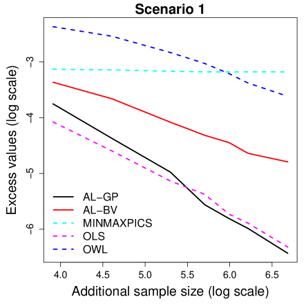
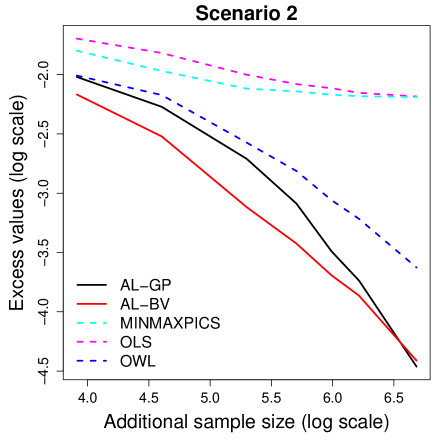
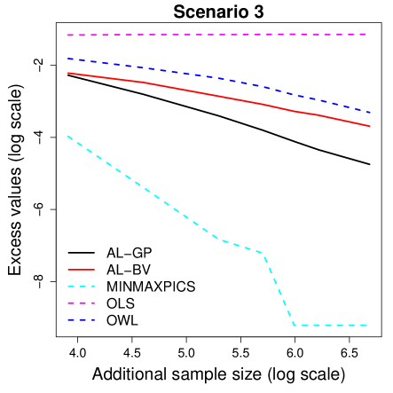
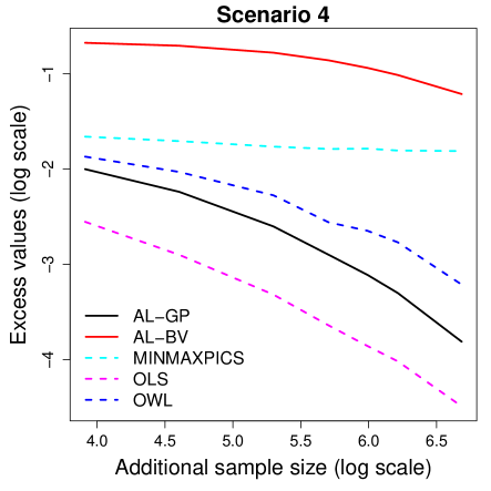
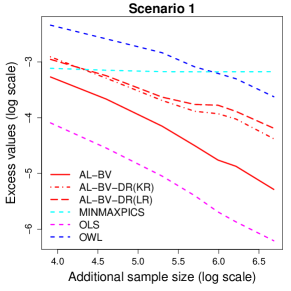
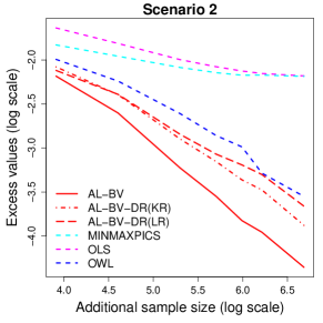
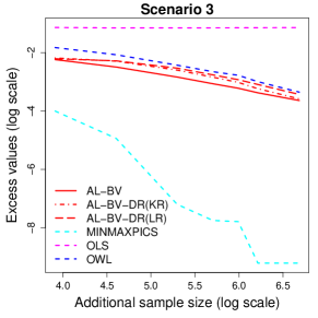
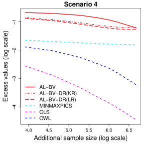
It can be seen that the optimal ITR for Scenario 1 is linear, i.e., ${D}^{*}(X)=\mbox{sign}(1-X_{1}-X_{2})$. The optimal ITR for Scenario 2 is nonlinear, with $D^{*}(X)=I(0.3\leq X_{1}^{2}+X_{2}^{2}\leq 1.7)$. Scenario 3 represents the case where the data are supported on the manifold, i.e., a two-dimensional sphere in $\mathbb{R}^{3}$. The treatment effect in Scenario 3 is highly nonlinear with $D^{*}(X)=\mbox{sign}(X_{1}X_{2}(1+X_{3}))$. Scenario 4 has a relatively high dimensional covariate, i.e., 8, with a linear treatment effect.

We apply the active clinical trial outlined in Algorithm 1. We implemented both the kernel method in Section 2.3.1, denoted AL-BV, and the Gaussian process regression method in Section 2.3.2, denoted AL-GP. We used the gpml Matlab toolbox (Rasmussen and Nickisch, 2010) in the latter method. The active clinical trial proceeds by selectively recruiting subjects whose differential treatment effects are smaller than a threshold, i.e., Steps 3–4 of Algorithm 1. This iterative procedure screens out a certain number of subjects, whose optimal treatments can be determined with high confidence, and retains the remaining $N$ subjects for estimating the optimal ITR. The active learning algorithm proposed in Deng et al. (2011a) serves as a comparison. The designed trial therein focuses on simple ITRs that utilize a small number of subpopulation categories to personalize the treatment. In particular, they assume the subpopulations are known a priori. Throughout the clinical trial, they sequentially select the (subpopulation, treatment) pair so as to minimize the maximal error of selecting a suboptimal treatment. For all the scenarios, we form four subgroups by dichotomizing $X_{1}$ and $X_{2}$ at 0. We use MINMAXPICS, the algorithm name in their paper, to denote this method.

In addition, we compare with two passive learning approaches: the outcome weighted learning (OWL) method (Zhao et al., 2012) and the ordinary least square (OLS) method. Both methods recruit subjects upon arrival in the clinical trial and estimate the optimal ITR using the collected data after the trial ends. $N$ subjects are randomly selected for both methods. In the OWL method, using the available data, we minimize the target function ${\mathbb{P}_{n}}\left[{R\phi(Af({X}))}/{\pi(A;{X})}\right]+\lambda_{n}\|f\|_{2}^{2},$ where $\phi(t)=\max(1-t,0)$ is the hinge loss, ${\mathbb{P}_{n}}$ is the empirical measure, and $\lambda_{n}$ is a tuning parameter controlling the amount of penalization. We consider a nonlinear functional space for the ITRs, and a Gaussian kernel is used in the implementation. The optimal ITR is estimated via $\widehat{D}({x})=\mbox{sign}(\widehat{f}(X))$, where $\widehat{f}(x)$ are the minimizers of the above objective function. In the OLS method, we first regress $R$ on $({X},A,{X}A)$, and then estimate the optimal ITR by finding the treatment that yields a larger predicted outcome for each individual.

The initial sample size $N_{0}$ is fixed at $50$, while the additional sample size $N-N_{0}$ is $50,100,200,300,400,500$, or $800$. To evaluate the empirical performance, we generated a testing dataset of sample size $10000$, mimicking a large pool of future subjects. The estimated ITRs $\widehat{D}(X)$ using the different methods are validated on this large testing set. Since the main effect is invariant across different ITRs, we can calculate the average excess value $AEV(D^{*},\widehat{D})$ as

$$AEV(D^{*},\widehat{D})=\frac{1}{n}\sum_{i=1}^{n}[T_{0}(X^{(i)},D^{*})-T_{0}(X^{(i)},\widehat{D})],\,\,n=10000$$

where the empirical average is taken over the validation set. This quantity directly reflects the expected clinical benefits for future subjects treated according to $\widehat{D}(X)$, with a smaller value indicating a better treatment decision. We repeat the process $1000$ times and average the resulting values over all the runs. In Figure 6, we plot $\log\{AEV(D^{*},\widehat{D})\}$ against $\log(N-N_{0})$, where $\widehat{D}$ was obtained using each method. The log-scale is used to give a better display of the polynomial convergence rates in the different methods.

In all the scenarios, our active clinical trials perform uniformly better than OWL. In Scenario 1, the treatment effect is linear, which indicates that OLS is the best possible method. However, AL-GP has comparable performance, especially when the sample size is large. The performance of AL-BV also improves with $N$. When the treatment effect is nonlinear, as in Scenarios 2 and 3, the strength of active learning is clearly demonstrated. Both methods initially perform better for small sample sizes and then converge much faster as the sample size grows. In contrast, the values of the estimated ITRs from the other two methods do not converge (Scenario 3) or do not converge to the optimal value (Scenario 2). In Scenario 4, the number of covariates is increased to eight. This places severe difficulties on the kernel estimation because of the curse of dimensionality. However, with the linear treatment effect, the AL-GP results are satisfactory compared with those of OLS. The MINIMAXPICS algorithm performs the best in Scenario 3, where the subpopulations are correctly defined in advance. When the prespecification of the subpopulations is incorrect, each subpopulation contains both patients who benefit from treatment 1 and patients who benefit from treatment -1. In this case, the constructed ITRs are not ideal, even with large sample sizes. In general, we believe that active learning methods provide robust results for various treatment mechanisms, which are usually unknown in practice. We presented some additional simulation results in the supplementary materials, where we investigated scenarios with biomarkers of normal distribution, and conducted several sensitivity analyses.

Figure 3: Excess values (log scale). Initial size was set to 50.

5 Real Data Analysis

5.1 Nefazodone–CBASP Clinical Trial

We apply the proposed active learning methods to analyze the data from the Nefazodone–CBASP clinical trial (Keller et al., 2000). The randomized trial was conducted to compare the efficacy of three treatments for nonpsychotic chronic major depressive disorder (MDD), namely Nefazodone, cognitive behavioral-analysis system of psychotherapy (CBASP), or a combination of Nefazodone and CBASP. CBASP requires twice-weekly on-site visits to the clinic, and thus imposes a significant burden on patients compared with Nefazodone alone. Hence, we compare Nefazodone with the combination treatment, and investigate whether CBASP is necessary for all patients. We perform a complete case analysis. The score on the 24-item Hamilton rating scale for depression (HRSD) was the primary outcome, with higher scores indicating more severe depression. Data from 441 patients were available, with 218 patients randomized to Nefazodone and 223 to the combined treatment group. We consider three covariates for tailoring the treatment: the baseline HRSD scores, the alcohol dependence, and the HAMA somatic anxiety scores. The latter two covariates were selected by Gunter et al. (2007) as important variables for optimal treatment decision making.

All the patients are used for the OLS and OWL analysis. To mimic an active clinical trial, we first randomly select 50 patients as the initial dataset. We then sequentially examine the remaining patients, and drop those who do not satisfy the selection criteria. The recruitment stops once an additional 300 patients are enrolled, or all the patients have been examined. The eligible patients are included in the dataset, assuming that they have been randomized in an active clinical trial. The treatments they are randomized to in this hypothetical active clinical trial are the actual treatments they received in the completed trial. In particular, 289 and 350 patients were used to construct the optimal ITRs using AL-BV and AL-GP respectively. The estimated ITRs from the different methods were applied to the whole data set to calculate the average HRSD scores due to the ITRs, with smaller values being preferable. Here, the “average HRSD scores due to the ITRs” are defined to be ${{\mathbb{P}_{n}}[\{\widetilde{R}I(A=D(X)\}/\pi(A)]}/{{\mathbb{P}_{n}}[\{I(A=D(X)\}/\pi(A)]},$ where $\widetilde{R}$ denotes the HRSD scores and $\pi(A)$ is the probability of being assigned treatment $A$. AL-BV recommends combination therapy for 299 patients, giving an average HRSD score of 8.86. AL-GP recommends this therapy for 386 patients, giving an average HRSD score of 9.72. OLS and OWL recommend this therapy for all the patients, yielding a higher score of 10.89. Hence, the treatment rules produced by the active clinical trials not only lead to a higher overall benefit, but also reduce the time and monetary commitments for the patients.

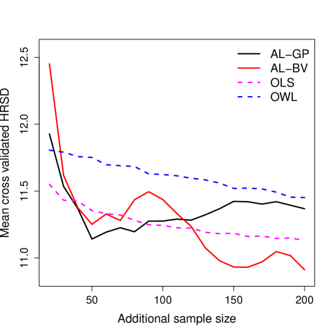
We then used a five-fold cross-validation analysis to avoid potential overfitting. The data set was partitioned into five subsets. Four of the five subsets were used as training data to construct the optimal ITR, and the remaining subset was used as the validation set to evaluate the estimated rule. In the training subset, we applied both active learning and passive learning methods, i.e., OLS and OWL, to construct the optimal ITRs. The initial sample size was set to 50 for the active learning methods. The number of additional recruited patients was $20,30,\ldots,200$; these were adaptively selected from the rest of the training samples. For the passive learning methods, we randomly chose $70,80,\ldots,250$ patients from the training data and conducted the estimation. The process was repeated 200 times, and we recorded the average cross-validated values for each sample size. The results are presented in Figure 4. The active learning methods initially lead to higher HRSD scores, but they catch up and continue to improve as the sample size grows. In particular, we can see that the HRSD scores from our methods decrease faster than those of the other methods do. After the additional sample size reaches 120, with the total sample size at 170, the ITR identified by AL-BV yields the lowest score, and this value can be further improved with larger sample sizes.

Figure 4: Mean cross-validated HRSD scores (the lower the better) against additional sample sizes. The initial sample size was set to 50.

5.2 Twelve-step Intervention on Stimulant Drug Use

These data come from a randomized clinical trial that aims to evaluate the effectiveness of 8-week group intervention plus individual 12-step facilitative intervention for reducing stimulant drug use (Donovan et al., 2013). Individuals with stimulant-use disorders were randomly assigned to treatment as usual (TAU) or to TAU integrated with Stimulant Abuser Groups to Engage in 12-step (STAGE-12) intervention.

The primary outcome of interest is the number of days of self-reported stimulant drug use over the three- to six-month post-randomization period, where a smaller value is preferable. We use seven baseline variables to evaluate the patients and to construct the optimal ITR: age, average number of days per month of self-reported stimulant drug use in the three months prior to randomization, baseline alcohol use, drug use, employment status, medical status, and psychiatric status composite scores on the addiction severity index (ASI), where the ASI composite score, ranging from 0 (no endorsement of any problems) to 1 (maximal endorsement of all problems), is usually taken as an indication of problem severity; it is perceived to guide the treatment decision (McGahan et al., 1986).

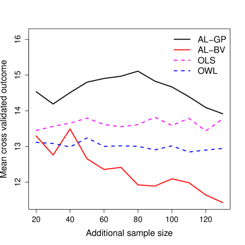
After removing the missing data, we have 305 participants in total. We evaluated the different methods on the whole data set, with the initial sample size set to 50 and the additional sample size set to 200. AL-BV and AL-GP assigned 123 and 90 patients to the STAGE-12 group, with expected outcomes of 11.3 and 12 respectively. OLS and OWL gave overall averages of 11.8 and 12.7 days. We also calculated the cross-validated number of days of drug use over the three- to six-month post-randomization period. Since the outcome was count data, with considerable zero-inflation, overdispersion, and a nonlinear trend, we anticipated that the active learning method using a bias-variance tradeoff for the estimation would lead to the best results. Indeed, as shown in Figure 5, AL-BV outperforms the other methods with a fast overall decreasing trend. While the Gaussian assumption is severely violated in this example, AL-GP still improves with sample size. We note that OLS and OWL do not improve noticeably as the sample size grows.

Figure 5: Mean cross-validated outcomes (number of days of self-reported stimulant drug use over the three- to six-month post-randomization period, the lower the better) against additional sample sizes. The initial sample size was set to 50.

6 Sample Size Consideration

In order to design a future study, it is important to plan ahead a sample size, which is sufficient to guarantee that we will obtain an ITR very close to the optimal one using the proposed active clinical trial. Here, we provide a data-driven method that gives a preliminary assessment of the required sample size. Further work is warranted to derive the sample size formula for such an exploratory trial. Let $V_{0}$ be an average patient outcome based on the standard care. Our goal is to determine a minimal sample size $N^{*}$ such that: (1) the power to reject the hypothesis $V({D}^{*})=V_{0}$ is at least $1-\beta$ when $V({D}^{*})\geq(1+\rho)V_{0}$; and (2) $Pr(|V(\hat{D}_{N^{*}})-V({D}^{*})|\leq\epsilon)\geq 1-\alpha$ (Laber et al., 2015), where $\epsilon$, $\alpha$, and $\rho$ are prespecified constants and $\hat{D}_{N}$ is the resulting estimator based on $N$ samples from the active clinical trial. Since we have constructed a non-asymptotic error bound for $|V(\hat{D}_{N})-V({D}^{*})|$ in terms of the sample size $N$ in Theorem 3.1, we suggest to obtain $N^{*}$ by inverting the above error bound such that $Pr(|V(\hat{D}_{N^{*}})-V({D}^{*})|\leq\min(\rho V_{0},\epsilon))\geq 1-\alpha.$ By doing so, we are able to provide finite sample evidence that the optimal individualized treatment rule yields a larger average benefit than the standard care, and, moreover, the average benefit of the estimated rule is approximately optimal. The constant $\gamma\in[0,d]$ will be determined based on prior knowledge, or can be set to a range of values to examine the resulting sample sizes. The unknown constant $\widetilde{C}$ can be determined via simulations. Given $d,\gamma,\theta$ and $\widetilde{C}$, the required sample size $N^{*}$, such that with probability greater than $1-\alpha$, $|V(\hat{D}_{N^{*}})-V({D}^{*})|\leq\min(\rho V_{0},\epsilon)$, can be found by setting $\widetilde{C}N^{*-\frac{1+\gamma}{2+d-\gamma}}\left(\log(N^{*}/\alpha)\right)^{\theta}=\min(\rho V_{0},\epsilon)$. The required sample sizes vary by the allocated initial sample size $N_{0}$. Therefore, our sample size calculation is conditional on a specified $N_{0}$. We will illustrate the proposed strategy by designing a future study to explore the optimal ITRs for patients with MDD. The Nefazodone-CBASP clinical trial is used as the basis for planning.

Consider two treatment options, Nefazodone only versus the combined treatment. The average HRSD score in the combined treatment group is 10.96. It is desirable to develop an ITR that can at least reduce the expected HRSD score that would be achieved by 15% with probability greater than 80%, i.e., $\rho V_{0}\approx 1.7$ and $\alpha=0.2$. We will use three tailoring variables with $d=3$.. To determine $\tilde{C}$, we adopt a bootstrap method. We will bootstrap the data, a total of 441 patients, 10000 times. An active clinical trial, with 50 initial and 100 additional patients, will be implemented with each bootstrapped sample to estimate the optimal ITR. The average HRSD score under each estimated ITR will be recorded. We denote these scores as $\hat{V}_{1}^{B},\ldots,\hat{V}_{10000}^{B}$. Let $k^{*}=\mbox{argmin}_{k=1,\ldots,10000}\hat{V}_{k}^{B}$. $\hat{V}_{k^{*}}^{B}$ will be used as an estimate of $V({D}^{*})$. Denote the 80 percentile of $|\hat{V}_{k}^{B}-\hat{V}_{k^{*}}^{B}|,k\neq k^{*},k=1,\ldots,10000$ as $\widehat{Diff}$. $\widetilde{C}$ can be obtained using $\tilde{C}=N^{\frac{1+\gamma}{2+d-\gamma}}\left(\log(N/\alpha)\right)^{-\theta}\times\widehat{Diff}$, where $N=150$ and $\alpha=0.2$. We will assess different $\gamma$’s with $\gamma=0.5,1,1.5,2,2.5$ and 3, which lead to different $\theta$’s and different estimates of $\widetilde{C}$. Using the outlined strategy, we suggest to plan the sample size for the future study according to Table 1.

$\epsilon$	$\gamma=0.5$	$\gamma=1$	$\gamma=1.5$	$\gamma=2$	$\gamma=2.5$
1.7	165	160	155	155	150
1.6	215	190	175	165	160
1.5	280	225	200	180	170

Table 1: Planned sample size for different combinations of $(\gamma,\epsilon)$.

7 Discussion

In this paper, we propose an active clinical trial with the goal of constructing favorable ITRs at a minimal cost. This new paradigm is distinct from the standard clinical trial framework that is designed for treatment evaluation. Along with the new designs, we also present new analysis and inference tools that are often practically useful and theoretically efficient. Two methods are presented to construct the confidence interval in the algorithm. The kernel smoothing method is better in the situation where a few important tailoring variables are known a priori. However, due to the curse of dimensionality, it cannot handle a covariate space of moderate to high dimension. The Gaussian process regression approach performs better in this situation. However, the kernel smoothing method does not assume a specific underlying distribution of the outcomes, whereas the Gaussian process regression approach requires the outcome to follow a Gaussian distribution, which may not be appropriate for discrete outcomes. Since the goal of the proposed trial is to explore the optimal treatment rules, it is a learning stage. The results should be further validated in a confirmatory trial.

In practice, we may also want to include individuals who would be known to benefit from the treatment. Instead of dropping certain patients whose confidence interval for the contrast function does not contain 0, we can enroll all patients with different priority (quantified by probability). Specifically, we can prioritize those patients, whose confidence interval of the contrast function contains 0, by assigning larger probabilities, while enrolling patients, whose confidence interval for the contrast function does not contain 0, with lower probabilities. Under this more flexible framework, individuals who benefit from the treatment are also included in the trial such that the marginal treatment effects can be investigated. In addition, when there is a small difference between two medications, treatment choice will likely depend on other considerations such as cost, side effects and etc. Our framework can take into account those factors that can be quantified. By allowing a ratio of the cost per treatment relative to the cost of a worse disease outcome, say $\delta$, which reflects the patients’ tolerance of treatment burden relative to tolerance of the disease burden (Vickers et al., 2007; Huang and Laber, 2014), we maximize $V(D)-\delta P(A=1)$. The optimal rule is instead given by $D^{*}(x)=\mbox{sign}\{f^{*}(x)-\delta\}$. In this case, the active clinical trial will enroll patients from whom the value of $f^{*}(x)$ is close to $\delta$, since these patients are close to the decision boundary and thus most informative.

We next discuss two directions for future research. First, our method can easily be extended to incorporate multi-category treatments, where patients are recruited based on the minimum differential treatment effect of all the pairwise comparisons. For continuous treatments, one possibility is to discretize the continuous treatment into different percentiles and then apply the extended method for multi-category treatments. Second, in this paper, we assume that the outcomes of the previous patients have been observed before we enroll the next patient. In fact, the proposed active clinical trials can be conducted with delayed responses, provided the required estimates (for the contrast function) can be updated as data become available, i.e., some responses can be collected during the study period. We can also update the estimates after groups of responses instead of individual responses. There have been some recent developments on handling the problem of delayed outcomes in phase I–II trials, for example, by treating them as missing values and applying imputation strategies (Jin et al., 2014). We would like to explore such options in the future. There are two other interesting extensions that we are pursuing: (i) a more general contrast function that can accommodate a high-dimensional or discrete covariate; (ii) a dynamic treatment regime for a sequence of treatment rules (Murphy, 2003; Robins, 2004).

Appendix A Technical Proofs

A.1 Intrinsic dimension of $\mbox{supp}(\Pi)$

We explain the meaning of “intrinsic dimension” introduced in Assumption (A3) here. We say that $\mbox{supp}(\Pi)$ possesses a tree decomposition $\mathcal{T}=\left\{T_{i,j},\ i\geq 1,\ j=1\ldots J(i)\right\}$ if

1. $T_{1,1}=\mbox{supp}(\Pi)$, and $\{T_{i,j}\}_{j=1}^{J(i)}$ forms a disjoint partition of $\mbox{supp}(\Pi)$ for all $i\geq 1$.

2. Nested partition: $\forall i\geq 2,j=1,\ldots,J(i)$, there exists a unique $1\leq k\leq J(i-1)$ such that $T_{i,j}\subset T_{i-1,k}$;

3. Bounded diameter: for all $i\geq 1,1\leq\ j\leq J(i)$,

   $${\rm diam}(T_{i,j}):=\sup_{x,y\in T_{i,j}}\|x-y\|_{2}\leq K_{1}2^{-i}$$

   for some $K_{1}=K_{1}(\Pi)$.

4. Regularity: for any $i\geq 1,1\leq j\leq J(i)$ and $0<r\leq 2^{-i}$ the following holds: there exists a $1\leq d\leq p$ ($d$ is the intrinsic dimension) such that for all $x\in T_{i,j}$,

   $$c_{1}r^{d}\leq\Pi(B(x,r)\cap T_{i,j})\leq c_{2}r^{d}$$ (A.1)

   for some $0<c_{1}(\Pi)\leq c_{2}(\Pi)<\infty$ which are independent of $i,j$. Here, $B(x,r)$ is the Euclidean ball of radius $r$ centered at $x$.

A simple example that gives a good intuition to the tree decomposition is the uniform distribution over the unit cube in $\mathbb{R}^{p}$. In this case, the tree decomposition is given by partitioning the unit cube into dyadic cubes and $d=p$. If $\mbox{supp}(\Pi)$ is contained in a proper subspace $W$ of $\mathbb{R}^{p}$, then $d\leq\dim(W)$.

Let $\mathcal{B}_{i}$ be the sigma-algebra generated by the collection of sets $\{T_{i,j},\ j=1,\ldots,J(i)\}$ (a partition of $\mbox{supp}(\Pi)$ on the level $i$). A regular approximation of ${\rm AS}_{k}$ in Algorithm 1 is given by ${\rm act}_{k}:=\bigcap\left\{A:\ A\in\mathcal{B}_{m_{k-1}},\ A\supset{\rm AS}_{k}\right\}$.

A.2 Properties of Kernel Estimate

A.2.1 Preliminaries

For a measurable set $S\subset\mbox{supp}(\Pi)$, define $\Pi_{S}(dx):=\Pi(dx|x\in S)$ as the conditional distribution on $S$, and set

$$\mathbb{Q}_{h}(x|S):=\int\limits_{\mathbb{R}^{p}}K_{h}\left({x-y}\right)d\Pi_{S}(y).$$

Since $\Pi$ is assumed to be known, we can directly compute $Q_{h}(x|S)$ now. Accordingly, we modify the original kernel estimate for $\eta_{j}$, i.e., (2.3), as follows: let $\{(X^{(i)},A^{(i)},R^{(i)}),\ i=1\ldots N\}$ be an i.i.d. sample from the conditional joint distribution of $(X,A,R)$ given that $X\in S$, and set

$$\widehat{\eta}_{j}(x;h,S)=\frac{1}{N}\sum\limits_{i=1}^{N}\frac{R^{(i)}I\{A^{(i)}=j\}K_{h}\left(x-X^{(i)}\right)}{Q_{h}(x|S)P(A^{(i)}=j)},\ j=\pm 1,$$ (A.2)

$$\widehat{f}(x;h,S)=\widehat{\eta}_{1}(x;h,S)-\widehat{\eta}_{-1}(x;h,S).$$

We will discuss properties of these estimators in below.

Let $h>0$, $S\in\mathcal{B}_{j}$ and $h\leq 2^{-j}$, and define

$$\mathbb{Q}_{h,m}(x|S):=\int\limits_{\mathbb{R}^{p}}\|x-y\|_{2}^{m}K_{h}\left({x-y}\right)d\Pi_{S}(y)$$ (A.3)

We next study the upper and lower bounds of $\mathbb{Q}_{h,m}(x|S)$ based on Assumptions (A1)-(A4). Since $K$ is bounded and compactly supported, there exists $R=R_{K}>0$ such that $K(x)\leq\|K\|_{\infty}I\{x\in B(0,R_{K})\}$. Let $F>0$ be a large enough constant, namely, $F^{d}\geq 2c_{2}/c_{1}$. Recall that $c_{1},c_{2}$ are defined in (A.1). Note that Assumption (A2) implies the following:

$$\mathbb{Q}_{h,m}(x|S) \geq\ell_{K}\int\limits_{B(x,h)\cap S}\|x-y\|_{2}^{m}d\Pi_{S}(y)$$

$$\geq\ell_{K}\left(h/F\right)^{m}\left(\int\limits_{B(x,h)\cap S}d\Pi_{S}(y)-\int\limits_{B(x,h/F)\cap S}d\Pi_{S}(y)\right)$$

$$\geq\ell_{K}\left(h/F\right)^{m}\frac{\left(c_{1}h^{d}-c_{2}(h/F)^{d}\right)}{\Pi(S)}\geq\frac{1}{2F^{m}}\ell_{K}c_{1}\frac{h^{d+m}}{\Pi(S)}:=c_{3}\frac{h^{d+m}}{\Pi(S)},$$ (A.4)

and

$$\mathbb{Q}_{h,m}(x|S)\leq \|K\|_{\infty}\int\limits_{B(x,R_{K}h)\cap A}\|x-y\|_{2}^{m}d\Pi_{S}(y)\leq\|K\|_{\infty}R_{K}^{m+d}c_{2}\frac{h^{d+m}}{\Pi(S)}:=c_{4}\frac{h^{d+m}}{\Pi(S)}.$$ (A.5)

In what follows, we will set $Q_{h}(x|S):=Q_{h,0}(x)$ for brevity.

A.2.2 Some bounds for the kernel estimators

In this subsection, we derive basic concentration inequalities for the kernel estimators of $\eta_{j}(x)=\mathbb{E}[R|A=j,X=x]$, $j=\pm 1$ restricted to $S$, i.e., $\widehat{\eta}_{j}(x;h,S)$ defined in (A.2). The proof of the results can be found in supplementary materials.

Lemma A.1.

For all $t>0$ satisfying $t+d^{2}\log(1/h)\leq nh^{d}$, with probability $\geq 1-2e^{-t}$,

$$\sup\limits_{x\in\mbox{supp}(\Pi)\cap S}|\widehat{\eta}_{j}(x;h)-\eta_{j}(x)|\leq C\left(h+\sqrt{\frac{\Pi(S)(t+d^{2}\log(1/h))}{nh^{d}}}\right),$$

where $C=C(M,c_{1},c_{2},L,L_{K},\|K\|_{\infty},\ell_{K},R_{K})$ is a constant.

The following Corollary is immediate:

Corollary A.1.

Set $h_{n}:=\left\{\Pi(S)(t+d\log(n/\Pi(S)))/n\right\}^{1/(d+2)}$. Then, under assumptions of Lemma A.1, with probability $\geq 1-4e^{-t}$,

$$\sup\limits_{x\in\mbox{supp}(\Pi)\cap S}|\widehat{f}(x;h_{n})-f^{\ast}(x)|\leq 4Ch_{n},$$

where constant $C$ is the same as in Lemma A.1.

A.3 Proof of Theorem 3.1

A.3.1 Comparison inequality

Our Lemma A.2 below illustrates the connection between the risk $V(\widehat{D})-V(D^{\ast})$ of a treatment rule $\widehat{D}(x)=\mbox{sign}(\widehat{f}(x))$ and the sup-norm $\|\widehat{f}-f^{\ast}\|_{\infty,\mbox{supp}(\Pi)}$.

Lemma A.2.

Under the margin assumption (A4),

$$V(\widehat{D})-V(D^{\ast})\leq C(\gamma)\|(\widehat{f}-f^{\ast})\mathcal{I}\left\{\mbox{sign}(\widehat{f})\neq\mbox{sign}(f^{\ast})\right\}\|_{\infty,\mbox{supp}(\Pi)}^{1+\gamma}.$$

Proof.

It is easy to see that $V(\widehat{D})-V(D^{\ast})=2\mathbb{E}\left(|f^{\ast}(X)|I\{\widehat{D}(X)\neq D^{\ast}(X)\}\right)$. The rest of the argument repeats Lemma 5.1 in Audibert and Tsybakov (2007). ∎

A.3.2 Main proof

Our main goal is to control the size of the set ${\rm act}_{k}$ defined by Algorithm 1. In turn, these bounds depend on the size of the confidence bands for $f^{\ast}(x)$ (denoted by $\delta_{k}$). Suppose $L\leq N$ is the number of iterations performed by the algorithm before termination.

Let $N_{k}^{{\rm act}}:=\lfloor N_{k}\cdot\Pi({\rm act}_{k})\rfloor$ be the number of labels requested on the $k$-th iteration of the algorithm. We first claim that the following bounds hold uniformly for all $1\leq k\leq L$ with probability at least $1-\alpha$:

$$\|f^{\ast}-\widehat{f}_{k}\|_{\infty,{\rm act}_{k}}\leq C_{1}\left(\frac{\log(N/\alpha)+d\log(N_{k})}{N_{k}}\right)^{1/(d+2)},$$

$$\Pi({\rm act}_{k})\leq C_{2}\left(\frac{\log(N/\alpha)+d\log(N_{k-1})}{N_{k-1}}\right)^{\gamma/(d+2)},$$ (A.6)

where $C_{j}=C_{j}(M,c_{1},c_{2},L,L_{K},\|K\|_{\infty},\ell_{K},R_{K},\gamma),\ j=1,2$. This claim will be proved later.

Let $\mathcal{E}$ be the event of probability $\geq 1-\alpha$ on which both inequalities of (A.3.2) hold, and assume that it occurs. Second inequality of (A.3.2) implies, together with the fact that $N_{k}=2N_{k-1}$ by definition, that the number of randomized subjects on each step $1\leq k\leq L$ satisfies

$$N_{k}^{{\rm act}}=\lfloor N_{k}\Pi({\rm act}_{k})\rfloor\leq 2N_{k-1}^{\frac{2+d-\gamma}{2+d}}\left(\log(N/\alpha)+d\log(N_{k-1})\right)^{\gamma/(d+2)}$$

with probability $\geq 1-\alpha$. If $N$ is the maximum number of randomized subjects the algorithm is allowed to request, then

$$N\leq \sum\limits_{k=0}^{L}N_{k}^{{\rm act}}\leq 2\left(\log(N/\alpha)+d\log(N_{L})\right)^{\gamma/(d+2)}\sum_{k=0}^{L}N_{k}^{\frac{2+d-\gamma}{2+d}}\leq$$

$$C_{3}(\gamma,d)\left(\log(N/\alpha)+d\log(N_{L})\right)^{\gamma/(d+2)}N_{L}^{\frac{2+d-\gamma}{2+d}},$$

and one easily deduces that on the last iteration $L$ we have

$$N_{L}\geq c(\gamma,\Pi,d)\left(\frac{N}{\log(N/\alpha)}\right)^{\frac{2+d}{2+d-\gamma}}.$$ (A.7)

Recall that $N_{L}$ is defined in Algorithm 1.

To obtain the risk bound of the theorem from (A.7), we apply Lemma A.2:

$$V(\widehat{D})-V(D^{\ast})\leq C(\gamma)\left\|(\widehat{f}_{L}-f^{\ast})\cdot I\left\{\mbox{sign}(\widehat{f}_{L})\neq D^{\ast}\right\}\right\|_{\infty,\mbox{supp}(\Pi)}^{1+\gamma}.$$ (A.8)

Since $\left\{\mbox{sign}(\widehat{f}_{L})\neq D^{\ast}\right\}\subseteq{\rm act}_{L}$ whenever bounds (A.3.2) hold, it remains to estimate $\|\widehat{f}_{L}-f^{\ast}\|_{\infty,{\rm act}_{L}}$. Recalling the first inequality of (A.3.2) once again (for $k=L$), we get

$$\|(\widehat{f}_{L}-f^{\ast})\|_{\infty,{\rm act}_{L}}\leq C_{1}\left(\frac{\log(N/\alpha)+d\log(N_{L})}{N_{L}}\right)^{1/(d+2)}\leq\widetilde{C}N^{-\frac{1}{2+d-\gamma}}\left(\log(N/\alpha)\right)^{q},$$

where $q=\frac{4+2d-\gamma}{(2+d)(2+d-\gamma)}$, which together with (A.8) yields the final result.

It remains to show both inequalities of (A.3.2). We start with the bound on $\|\widehat{f}_{k}-f^{\ast}\|_{\infty,{\rm act}_{k}}$. First, note that by construction, for every $k\geq 1$ the samples $(X^{(i,k)},A^{(i,k)},R^{(i,k)}),\ i=1\ldots\lfloor N_{k}\Pi({\rm act}_{k})\rfloor$ are conditionally independent given the data $\bigcup_{i=1}^{k-1}S_{i}$ collected on steps $1,\ldots,k-1$, with conditional distribution of $X^{(i,k)}$ being $\Pi_{{\rm act}_{k}}$. Thus we can apply Corollary A.1 conditionally on $\bigcup_{i=1}^{k-1}S_{i}$ with $t=\log\frac{4N}{\alpha}$ to get that with probability $\geq 1-\alpha/N$,

$$\|\widehat{f}_{k}-f^{\ast}\|_{\infty,{\rm act}_{k}}\leq 4C\left(\frac{\log\frac{\alpha}{4N}+d\log(\lfloor N_{k}\Pi({\rm act}_{k})\rfloor/\Pi({\rm act}_{k}))}{\lfloor N_{k}\Pi({\rm act}_{k})\rfloor/\Pi({\rm act}_{k})}\right)^{1/(d+2)}\leq 8Ch_{k}.$$

It remains to integrate the bound with respect to the distribution of $\bigcup_{i=1}^{k-1}S_{i}$:

$$P\left(\|\widehat{f}_{k}-f^{\ast}\|_{\infty,{\rm act}_{k}}\geq 8Ch_{k}\right)=\mathbb{E}P\left(\|\widehat{f}_{k}-f^{\ast}\|_{\infty,{\rm act}_{k}}\geq 8Ch_{k}\,\big{|}\,\bigcup_{i=1}^{k-1}S_{i}\right)\leq\frac{\alpha}{N}.$$

The union bound over all $1\leq k\leq L\leq N$ gives the result.

Finally, we will prove the second inequality of (A.3.2), the bound for the size of the active sets ${\rm act}_{k}$. This is the place where assumption (A3) on the tree decomposition and margin assumption (A4) play the key role. To obtain the bound, we will compare two estimators of $f^{\ast}$: the first is the kernel estimator $\widehat{f}_{k}$ constructed by the Algorithm 1 on step $k$, and the second is the piecewise-constant estimator $\bar{f}_{k}$ with similar approximation properties to $\widehat{f}_{k}$. Namely, $\bar{f}_{k}$ is the $L_{2}(\Pi)$ - projection of $f^{\ast}$ on the linear space of piecewise-constant functions of the form $g(x)=\sum\limits_{j=1}^{J(m_{k})}\alpha_{j}I\{T_{m_{k},j}\}(x),\ \alpha_{j}\in\mathbb{R}$. Recall that $T_{i,j}$ is defined in the tree decomposition of Section A.1. As a result, we will be able to relate the “active sets” associated to these estimators, taking advantage of the fact that the active set associated to $\bar{f}_{k}$ is always a union of the sets from a collection $\{T_{m_{k},j},\ j=1\ldots J(m_{k})\}$.

Let $\mathcal{E}_{1}$ be the event of probability $\geq 1-\alpha$ on which $\|\widehat{f}_{k}-f^{\ast}\|_{\infty,{\rm act}_{k}}\leq\delta_{k}$ for any $k\geq 0$, where $\delta_{k}=4Ch_{k}$. Assume that $\mathcal{E}_{1}$ occurs.

The following inclusions hold (for the definition of $AS_{k+1}$, see Algorithm 1):

$$\left\{x:|f^{\ast}(x)|<\delta_{k}/2\right\}\subseteq AS_{k+1}\subseteq\left\{x:|f^{\ast}(x)|<5\delta_{k}/2\right\}.$$ (A.9)

Indeed,

$$|f^{\ast}(x)|<\delta_{k}/2\implies|\widehat{f}_{k}(x)|<\delta_{k}/2+|f^{\ast}(x)-\widehat{f}_{k}(x)|<\frac{3}{2}\delta_{k}\implies x\in AS_{k+1}$$

and

$$x\in AS_{k+1}\implies|\widehat{f}_{k}(x)|<\frac{3}{2}\delta_{k}\implies|f^{\ast}(x)|<\frac{5}{2}\delta_{k}.$$

For all $x\in T_{m_{k},j}$, set $\bar{f}_{k}(x):=\frac{1}{\Pi(T_{m_{k},j})}\int\limits_{T_{m_{k},j}}f^{\ast}(y)d\Pi(y)$, and note that

$$|f^{\ast}(x)-\bar{f}_{k}(x)|\leq \frac{1}{\Pi(T_{m_{k},j})}\int\limits_{T_{m_{k},j}}|f^{\ast}(y)-f^{\ast}(x)|d\Pi(y)\leq\frac{2L}{\Pi(T_{m_{k},j})}\int\limits_{T_{m_{k},j}}|x-y|d\Pi(y)\leq$$

$$2L\,{\rm diam}(T_{m_{k},j})\leq 2LK_{1}2^{-m_{k}}\leq 4LK_{1}h_{k},$$

where the last two inequalities follow from part 3 of assumption (A3) given in Appendix A.1, and from the definition of $m_{k}$. Define $\tau_{k}:=\max\left(5\delta_{k},4LK_{1}h_{k}\right)\leq C_{5}\delta_{k}$, $\bar{\mathcal{F}}_{k+1}:=\{f:\ |f(x)-\bar{f}_{k}(x)|\leq(3/2)\tau_{k},\ \forall x\in{\rm act}_{k}\}$ to be the band of size $(3/2)\tau_{k}$ around $\bar{f}_{k}$, and

$$\bar{A}_{k+1}:=\left\{x\in{\rm act}_{k}:\ \exists f_{1},f_{2}\in\bar{\mathcal{F}}_{k+1},\mbox{sign}(f_{1}(x))\neq\mbox{sign}(f_{2}(x))\right\}.$$

By a reasoning similar to above, we have the inclusions

$$\left\{x:|f^{\ast}(x)|<\tau_{k}/2\right\}\subseteq\bar{A}_{k+1}\subseteq\left\{x:|f^{\ast}(x)|<5\tau_{k}/2\right\}.$$ (A.10)

Moreover, by the definition of $\tau_{k}$, we have the inequality $5\delta_{k}/2\leq\tau_{k}/2$. Hence (A.9,A.10) imply that $AS_{k+1}\subseteq\bar{A}_{k+1}$. It remains to note that

1. $\bar{A}_{k+1}$ is the union of the sets from a collection $\{T_{m_{k},j},\ j=1\ldots J(m_{k})\}$, hence $\bar{A}_{k+1}\supseteq{\rm act}_{k+1}$;

2. By (A.10) and assumption (A4),

   $$\Pi({\rm act}_{k+1})\leq\Pi(\bar{A}_{k+1})\leq\Pi(\left\{x:|f^{\ast}(x)|<5\tau_{k}/2\right\})\leq K_{2}(5\tau_{k}/2)^{\gamma}\leq C_{6}\delta_{k}^{\gamma},$$

   hence proving the claim.

Supplementary Materials for “Active Clinical Trials for Personalized Medicine”

S.1 Additional simulation results

S.1.1 Simulation setups with normal biomarkers

In this section, we first present two additional examples where biomarkers have normal distributions (Scenarios 5 and 6). Particularly, $X_{1}$ and $X_{2}$ are generated according to $N(0,1)$. Treatments $A_{1}$, $A_{2}$ are randomly generated from $\{-1,1\}$ with equal probability 0.5. Outcomes $R$ are generated as follows.

1. $R\sim N(1+2X_{1}+0.5(X_{1}^{2}-0.25)A,1);$

2. $R\sim N(1+2X_{1}^{2}+X_{2}+2(\log(|X_{2}|)+\sqrt{|X_{1}|}-1)A,1).$

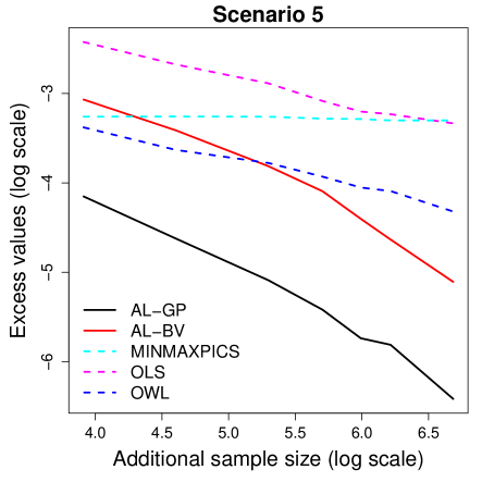
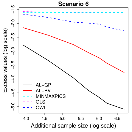
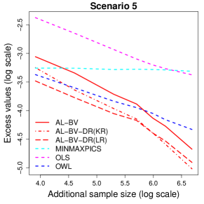
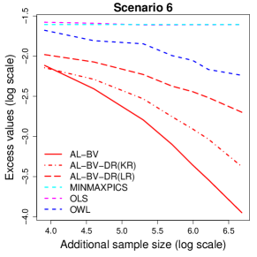
The results are presented in Figure 6. The outcome models are fairly complex in both scenarios. Hence the results from OLS are unsatisfactory. We prespecify 4 subgroups, with $X_{1}$ and $X_{2}$ dichotomized at 0, to implement the approach proposed in Deng et al. (2011a). Since these pre-specified subgroups are incorrect to inform the optimal treatment rule, the ITRs estimated by their approach are not consistent for the optimal. Both active learning methods show competitive performances in both scenarios. Kernel approach performs slightly worse than the Gaussian process regression. This phenomenon is anticipated since the bounded support assumption required in theoretical guarantee is violated.

Figure 6: Excess values (log scale). Initial size was set at 50.

S.1.2 Sensitivity analysis

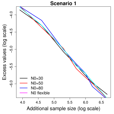
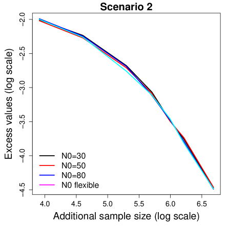
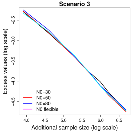
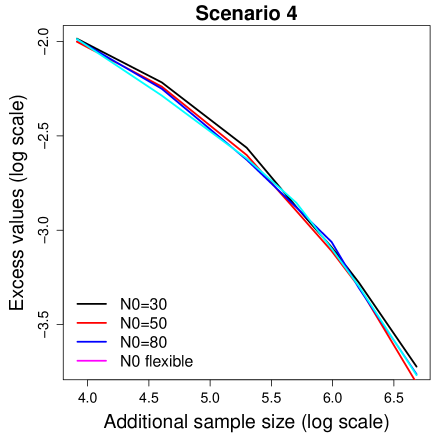
In this section, we conduct a thorough sensitivity analysis to investigate whether the performances of the proposed methods depend on the choices of initial sample size $N_{0}$. Basically, any number that is “significantly smaller” than the total allocated budget should lead to the same theoretical asymptotic behavior. Indeed, we vary $N_{0}$ from 30, 50 to 80 and find that the results are insensitive to the choice. We present the sensitivity analyses for Gaussian process regression method in Figure 7. The results for kernel approach are similar (data not shown).

We also investigate how the confidence level $\delta(x_{0})$ in the step of Algorithm 1 affects the performance of the algorithm. The confidence level $\delta(x_{0})$ is controlled by the parameter $t$, where $\delta(x_{0})=tLh_{n}(x_{0})$. We vary $t$ over the set $\{0.3,0.5,0.8,1\}$, and implicitly assume $L=1$. The results presented in Figure 8 clearly show that algorithm performances are robust to the choice of the confidence parameter.

Figure 7: Excess values (log scale) with different initial sizes in Gaussian process regression method. ‘N0 flexible’ means $N_{0}=2\lfloor\sqrt{n}\rfloor$.

Figure 8: Excess values (log scale) with different confidence parameters in kernel method. Initial size was set at 50.

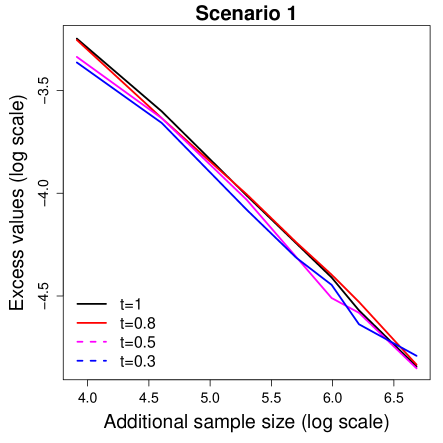
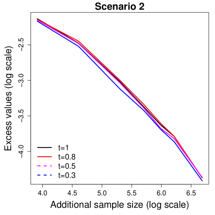
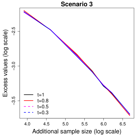
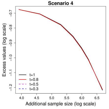
S.1.3 Doubly-robust estimator

The individualized treatment rule can also be constructed via a doubly robust augmented inverse probability weighted estimator. Here we examine the performance of such an estimator, which is used for estimation and participant inclusion in the active clinical trial. A doubly robust representation for the value function $V(D)$ is

$$V^{AIPWE,m}(D)\triangleq E\left[\frac{RI\left\{A=D(X)\right\}}{{\pi}^{m}(A;X)}-\frac{I\left\{A=D(X)\right\}-{\pi}^{m}\{D(X);X\}}{{\pi}^{m}\{D(X);X\}}{Q}^{m}\{X,D(X)\}\right],$$

where $\pi^{m}(a;x)$ denotes a working model for $P(A=a|X=x)$ and $Q^{m}(x,a)$ denotes a working model for $E(R|X=x,A=a)$. It can be shown that $V^{AIPWE,m}(D)=V(D)$ when either $\pi^{m}(a;x)$ or $Q^{m}(x,a)$ is correctly specified (Zhang et al., 2012). Denote

$$W_{a}^{m}=I(A=a)\frac{R-Q^{m}(X,a)}{\pi^{m}(a;X)}+Q^{m}(X,a).$$

The optimal treatment rule maximizing $V^{AIPWE,m}(D)$ is

$$D^{*}(x)=\mbox{sign}\{E(W_{1}^{m}|X=x)-E(W_{-1}^{m}|X=x)\}.$$

Within the framework of active clinical trial, patients for whom the difference between $E(W_{a}^{m}|X=x),a=\pm 1$, is small are more likely to get enrolled, since they are closer to the decision boundary. In the implementation, $\pi^{m}(a;x)=1/2$ is known. We can plug in the estimated $E(R|X=x,A=a)$ to estimate $E(W_{a}^{m}|X=x)$. Subsequently, the estimated $E(W_{1}^{m}|X=x)-E(W_{-1}^{m}|X=x)$ can be used to select enrolled patients. We examine the performance of active clinical trial based on a doubly robust estimator, where $E(R|X=x,A=a)$ are estimated using either kernel regression method (‘AL-BV-DR (KR)’) or a simple linear regression with $(X,A,XA)$ as predictors (‘AL-BV-DR (LR)’). Results for Scenarios 1-6 are shown in Figure 9. These results are relatively insensitive to the choices of working models for $Q^{m}(x,a)$. However, the performances of the doubly robust estimators vary across different situations. This might be due to a larger variability from using the doubly robust estimators with more estimation required. It will be of interest to further investigate the properties of active clinical trial via doubly robust estimators.

Figure 9: Excess values (log scale), ’AL-BV’ denotes the approach using the kernel smoothing estimator. ’AL-BV-DR (KR)’ denotes the approach based on a doubly robust estimator using kernel regression for $Q^{m}(x,a)$ and ’AL-BV-DR (LR)’ denotes the approach based on a doubly robust estimator using linear regression for $Q^{m}(x,a)$.

S.2 Additional theoretical results

Proof of Lemma A.1

We prove Lemma A.1 here. Below is the usual “bias-variance” decomposition

$$\|\widehat{\eta}_{j}(x;h)-\eta_{j}(x)\|_{\infty}\leq\|\widehat{\eta}_{j}(x;h)-\mathbb{E}\widehat{\eta}_{j}(x;h)\|_{\infty}+\|\eta_{j}(x)-\mathbb{E}\widehat{\eta}_{j}(x;h)\|_{\infty}.$$

We start with a bound on the bias term. Note that for any $x\in S\cap\mbox{supp}(\Pi)$, $\mathbb{E}\widehat{\eta}_{j}(x;h)=\frac{1}{Q_{h}(x|S)}\int K\left(\frac{x-y}{h}\right)\eta_{j}(y)d\Pi_{S}(y)$, hence

$$\left|\widehat{\eta}_{j}(x;h)-\mathbb{E}\widehat{\eta}_{j}(x;h)\right|=\left|\frac{1}{Q_{h}(x|S)}\int(\eta(x)-\eta(y))K\left(\frac{x-y}{h}\right)d\Pi(y)\right|\leq$$

$$\frac{L}{Q_{h}(x|S)}\int\|x-y\|_{2}K\left(\frac{x-y}{h}\right)d\Pi_{S}(y)=L\frac{Q_{h,1}(x|S)}{Q_{h}(x|S)}\leq L\frac{c_{4}}{c_{3}}h,$$ (A.11)

where $c_{3},c_{4}$ are defined in Section A.3.1. Recall that $Q_{h,1}(x|S)$ is defined in (A.3) with

$$\mathbb{Q}_{h,1}(x|S):=\int\limits_{\mathbb{R}^{p}}\|x-y\|_{2}K_{h}\left({x-y}\right)d\Pi_{S}(y).$$

Next, we will bound the stochastic term. Given $\varepsilon>0$, let $\{x^{(k)}\}_{k=1}^{N(\varepsilon)}$ be the minimal $\varepsilon$-net on $S\cap\mbox{supp}(\Pi)$, so that for any $y\in S\cap\mbox{supp}(\Pi)$ there exists $1\leq k(y)\leq N(\varepsilon)$ such that $\|y-x^{(k(y))}\|_{2}\leq\varepsilon$. Set $\varepsilon:=h^{d+1}$. Then

$$\sup\limits_{y\in S\cap\mbox{supp}(\Pi)}|\widehat{\eta}_{j}(y;h)-\eta_{j}(y)|=$$ (A.12)

$$\sup_{y\in S\cap\mbox{supp}(\Pi)}|\widehat{\eta}_{j}(y;h)-\widehat{\eta}_{j}(x^{(k(y))};h)+\widehat{\eta}_{j}(x^{(k(y))};h)-\eta_{j}(x^{(k(y))})+\eta_{j}(x^{(k(y))})-\eta_{j}(y)|\leq$$

$$\max_{1\leq i\leq N(\varepsilon)}|\widehat{\eta}_{j}(x^{(i)};h)-\eta_{j}(x^{(i)})|+\sup_{\|x-y\|_{2}\leq\varepsilon}|\eta_{j}(x)-\eta_{j}(y)|+\sup_{\|x-y\|_{2}\leq\varepsilon}|\widehat{\eta}_{j}(x;h)-\widehat{\eta}_{j}(y;h)|.$$

Lipschitz condition on $\eta_{j}$ implies that

$$\sup_{\|x-y\|_{2}\leq h^{d+1}}|\eta_{j}(x)-\eta_{j}(y)|\leq Lh^{d+1}$$

and, since $|R|\leq M$ almost surely and $K$ has Lipschitz constant $L_{K}$,

$$\sup_{\|x-y\|_{2}\leq h^{d+1}}|\widehat{\eta}_{j}(x;h)-\widehat{\eta}_{j}(y;h)|\leq\frac{ML_{K}\Pi(S)}{c_{3}h^{d}}\varepsilon=\frac{ML_{K}\Pi(S)}{c_{3}}h.$$

Fix $1\leq i\leq N(\varepsilon)$. We will apply the Bernstein’s inequality (e.g., Lemma 2.2.9 in van der Vaart and Wellner (1996)) to estimate $|\widehat{\eta}_{j}(x_{i};h)-\mathbb{E}\widehat{\eta}_{j}(x_{i};h)|$. Our assumptions imply that for all $1\leq i\leq N$,

$$\left|R^{(i)}I\{A^{(i)}=j\}\frac{K_{h}\left(x-X^{(i)}\right)}{Q_{h}(x|S)P(A^{(i)}=j)}\right|\leq\frac{2M\|K\|_{\infty}\Pi(S)}{c_{3}h^{d}}$$

almost surely, hence

$$\left|R^{(i)}I\{A^{(i)}=j\}\frac{K_{h}\left({x-X^{(i)}}\right)}{Q_{h}(x|S)P(A^{(i)}=j)}-\mathbb{E}R^{(i)}I\{A^{(i)}=j\}\frac{K_{h}\left({x-X^{(i)}}\right)}{Q_{h}(x|S)P(A^{(i)}=j)}\right|\leq\frac{4M\|K\|_{\infty}\Pi(S)}{c_{3}h^{d}}$$

almost surely for all $x\in S\cap\mbox{supp}(\Pi)$. Moreover, (A.4) implies that

$${\rm Var}\left(\widehat{\eta}_{j}(x;h)\right)\leq\frac{2M^{2}\|K\|_{\infty}}{n}\int\frac{K\left(\frac{x-y}{h}\right)}{Q^{2}_{h}(x|S)}d\Pi_{S}(y)\leq\frac{2M^{2}\|K\|_{\infty}\Pi(S)}{c_{3}nh^{d}}.$$

Bernstein’s inequality implies that for all $t>0$,

$$|\widehat{\eta}_{j}(x^{(i)};h)-\mathbb{E}\widehat{\eta}_{j}(x^{(i)};h)|\leq 2\max\left(M\sqrt{\frac{2\|K\|_{\infty}\Pi(S)t}{c_{3}nh^{d}}},4\frac{M\|K\|_{\infty}t}{c_{3}nh^{d}}\right)$$

with probability $\geq 1-2e^{-t}$. Combined with the union over all $1\leq i\leq N(\varepsilon)$ and noting that $N(\varepsilon)\leq\frac{C\Pi(S)}{\varepsilon^{d}}$, we get that

$$\max_{1\leq i\leq N(\varepsilon)} |\widehat{\eta}_{j}(x^{(i)};h)-\mathbb{E}\widehat{\eta}_{j}(x^{(i)};h)|\leq$$

$$C\max\left(M\sqrt{\frac{2\|K\|_{\infty}\Pi(S)(t+d^{2}\log(1/h))}{c_{3}nh^{d}}},2\sqrt{2}\frac{M\|K\|_{\infty}\Pi(S)(t+d^{2}\log(1/h))}{c_{3}nh^{d}}\right)$$

with probability $\geq 1-2e^{-t}$. Combined with (S.2 Additional theoretical results) and (A.12), this implies the result.

References

- Allard et al. (2012) Allard, W. K., Chen, G., and Maggioni, M. “Multi-scale geometric methods for data sets II: Geometric multi-resolution analysis.” Applied and Computational Harmonic Analysis, 32(3):435–462 (2012).
- Audibert and Tsybakov (2007) Audibert, J.-Y. and Tsybakov, A. B. “Fast learning rates for plug-in classifiers.” The Annals of statistics, 35(2):608–633 (2007).
- Balcan et al. (2008) Balcan, M.-F., Hanneke, S., and Wortman, J. “The True Sample Complexity of Active Learning.” In Proceedings of the Conference on Learning Theory, 45–56 (2008).
- Cai et al. (2011) Cai, T., Tian, L., Wong, P. H., and Wei, L. “Analysis of randomized comparative clinical trial data for personalized treatment selections.” Biostatistics, 12(2):270–282 (2011).
- Castro and Nowak (2008) Castro, R. M. and Nowak, R. D. “Minimax bounds for active learning.” Information Theory, IEEE Transactions on, 54(5):2339–2353 (2008).
- Cui et al. (2002) Cui, L., James Hung, H., Wang, S. J., and Tsong, Y. “Issues related to subgroup analysis in clinical trials.” Journal of biopharmaceutical statistics, 12(3):347–358 (2002).
- Dasgupta et al. (2007) Dasgupta, S., Monteleoni, C., and Hsu, D. J. “A general agnostic active learning algorithm.” In Advances in neural information processing systems, 353–360 (2007).
- Deng et al. (2007) Deng, K., Bourke, C., Scott, S., Sunderman, J., and Zheng, Y. “Bandit-Based Algorithms for Budgeted Learning.” In Proceedings of the 2007 Seventh IEEE International Conference on Data Mining, 463–468. IEEE Computer Society (2007).
- Deng et al. (2011a) Deng, K., Pineau, J., and Murphy, S. “Active learning for developing personalized treatment.” In Proceedings of the Twenty-seventh Conference on Uncertainty in Artificial Intelligence, 161–168 (2011a).
- Deng et al. (2011b) —. “Active learning for personalizing treatment.” In 2011 IEEE Symposium on Adaptive Dynamic Programming And Reinforcement Learning (ADPRL), 32–39. IEEE (2011b).
- DiMasi et al. (2010) DiMasi, J. A., Feldman, L., Seckler, A., and Wilson, A. “Trends in risks associated with new drug development: success rates for investigational drugs.” Clinical Pharmacology & Therapeutics, 87(3):272–277 (2010).
- Donovan et al. (2013) Donovan, D. M., Daley, D. C., Brigham, G. S., Hodgkins, C. C., Perl, H. I., Garrett, S. B., Doyle, S. R., Floyd, A. S., Knox, P. C., Botero, C., et al. “Stimulant abuser groups to engage in 12-Step: A multisite trial in the National Institute on Drug Abuse Clinical Trials Network.” Journal of Substance Abuse Treatment, 44(1):103–114 (2013).
- Foster et al. (2011) Foster, J. C., Taylor, J. M., and Ruberg, S. J. “Subgroup identification from randomized clinical trial data.” Statistics in medicine, 30(24):2867–2880 (2011).
- Gunter et al. (2007) Gunter, L., Zhu, J., and Murphy, S. “Variable selection for optimal decision making.” In Artificial Intelligence in Medicine, 149–154. Springer (2007).
- Hamburg and Collins (2010) Hamburg, M. and Collins, F. “The path to personalized medicine.” N Engl J Med., 363(4):301–304 (2010).
- Hanneke (2011) Hanneke, S. “Rates of convergence in active learning.” The Annals of Statistics, 39(1):333–361 (2011).
- Hu and Rosenberger (2006) Hu, F. and Rosenberger, W. F. The theory of response-adaptive randomization in clinical trials. New York: Wiley (2006).
- Huang and Laber (2014) Huang, Y. and Laber, E. “Personalized Evaluation of Biomarker Value: A Cost-Benefit Perspective.” Statistics in Biosciences, 1–23 (2014).
- Jin et al. (2014) Jin, I. H., Liu, S., Thall, P. F., and Yuan, Y. “Using Data Augmentation to Facilitate Conduct of Phase I-II Clinical Trials with Delayed Outcomes.” Journal of the American Statistical Association (2014). In press.
- Keller et al. (2000) Keller, M. B., Mccullough, J. P., Klein, D. N., Arnow, B., Dunner, D. L., Gelenberg, A. J., Markowitz, J. C., Nemeroff, C. B., Russell, J. M., Thase, M. E., Trivedi, M. H., and Zajecka, J. “A Comparison of Nefazodone, The Cognitive Behavioral-Analysis System of Psychotherapy, and Their Combination for the Treatment of Chronic Depression.” The New England Journal of Medicine, 342(20):1462–70 (2000).
- Koltchinskii (2010) Koltchinskii, V. “Rademacher complexities and bounding the excess risk in active learning.” The Journal of Machine Learning Research, 11:2457–2485 (2010).
- Laber et al. (2015) Laber, E., Zhao, Y.-Q., Regh, T., Davidian, M., Tsiatis, A., Stanford, J. B., Zeng, D., Song, R., and Kosorok, M. R. “Sizing a phase II trial to find a nearly optimal personalized treatment strategy.” (2015). Submitted.
- Lagakos (2006) Lagakos, S. W. “The challenge of subgroup analyses-reporting without distorting.” New England Journal of Medicine, 354(16):1667–1669 (2006).
- Little et al. (2009) Little, A. V., Jung, Y.-M., and Maggioni, M. “Multiscale Estimation of Intrinsic Dimensionality of Data Sets.” In AAAI Fall Symposium: Manifold Learning and Its Applications, 26–33 (2009).
- Madani et al. (2004) Madani, O., Lizotte, D. J., and Greiner, R. “The budgeted multi-armed bandit problem.” In Shawe-Taylor, J. and Singer, Y. (eds.), Learning Theory, 643–645. Springer (2004).
- McGahan et al. (1986) McGahan, P., Griffith, J., Parente, R., and McLellan, A. “Addiction severity index composite scores manual.” Philadelphia, PA: Treatment Research Institute (1986).
- Minsker (2012) Minsker, S. “Plug-in Approach to Active Learning.” Journal of Machine Learning Research, 13:67–90 (2012).
- Murphy (2003) Murphy, S. A. “Optimal Dynamic Treatment Regimes.” Journal of the Royal Statistical Society, Series B, 65:331–366 (2003).
- Qian and Murphy (2011) Qian, M. and Murphy, S. A. “Performance Guarantees for Individualized Treatment Rules.” The Annals of Statistics, 39:1180–1210 (2011).
- Raghavan et al. (2006) Raghavan, H., Madani, O., and Jones, R. “Active learning with feedback on features and instances.” The Journal of Machine Learning Research, 7:1655–1686 (2006).
- Rasmussen and Nickisch (2010) Rasmussen, C. E. and Nickisch, H. “Gaussian processes for machine learning (GPML) toolbox.” J. Mach. Learn. Res., 11:3011–3015 (2010).
- Rasmussen and Williams (2006) Rasmussen, C. E. and Williams, C. K. I. Gaussian processes for machine learning. Adaptive Computation and Machine Learning. Cambridge, MA: MIT Press (2006).
- Robbins (1952) Robbins, H. “Some Aspects of the Sequential Design of Experiments.” Bulletin of the American Mathematical Society, 58:527–535 (1952).
- Robins (2004) Robins, J. M. “Optimal Structural Nested Models for Optimal Sequential Decisions.” In Proceedings of the Second Seattle Symposium on Biostatistics, 189–326. Springer (2004).
- Rosenberger and Lachin (1993) Rosenberger, W. F. and Lachin, J. M. “The use of response-adaptive designs in clinical trials.” Controlled clinical trials, 14(6):471–484 (1993).
- Rosenberger et al. (2012) Rosenberger, W. F., Sverdlov, O., and Hu, F. “Adaptive randomization for clinical trials.” Journal of biopharmaceutical statistics, 22(4):719–736 (2012).
- Simon and Simon (2013) Simon, N. and Simon, R. “Adaptive enrichment designs for clinical trials.” Biostatistics, 14(4):613–625 (2013).
- Singer (2005) Singer, E. “Personalized medicine prompts push to redesign clinical trials.” Nature Medicine, 11(5):462–462 (2005).
- Tsybakov (2004) Tsybakov, A. “Optimal aggregation of classifiers in statistical learning.” The Annals of Statistics, 32(1):135–166 (2004).
- van der Vaart and Wellner (1996) van der Vaart, A. and Wellner, J. Weak convergence and empirical processes: with applications to statistics. Springer (1996).
- Vickers et al. (2007) Vickers, A. J., Kattan, M. W., and Sargent, D. J. “Method for evaluating prediction models that apply the results of randomized trials to individual patients.” Trials, 8(1):14 (2007).
- Wang et al. (2009) Wang, S.-J., James Hung, H., and O’Neill, R. T. “Adaptive patient enrichment designs in therapeutic trials.” Biometrical Journal, 51(2):358–374 (2009).
- Zhang et al. (2012) Zhang, B., Tsiatis, A. A., Laber, E. B., and Davidian, M. “A Robust Method for Estimating Optimal Treatment Regimes.” Biometrics, 68:1010–1018 (2012).
- Zhao et al. (2012) Zhao, Y. Q., Zeng, D., Rush, A. J., and Kosorok, M. R. “Estimating Individualized Treatment Rules using Outcome Weighted Learning.” Journal of American Statistical Association, 107:1106–1118 (2012).