Iterative structure of finite loop integrals

Abstract

In this paper we develop further and refine the method of differential equations for computing Feynman integrals. In particular, we show that an additional iterative structure emerges for finite loop integrals. As a concrete non-trivial example we study planar master integrals of light-by-light scattering to three loops, and derive analytic results for all values of the Mandelstam variables $s$ and $t$ and the mass $m$. We start with a recent proposal for defining a basis of loop integrals having uniform transcendental weight properties and use this approach to compute all planar two-loop master integrals in dimensional regularization. We then show how this approach can be further simplified when computing finite loop integrals. This allows us to discuss precisely the subset of integrals that are relevant to the problem. We find that this leads to a block triangular structure of the differential equations, where the blocks correspond to integrals of different weight. We explain how this block triangular form is found in an algorithmic way. Another advantage of working in four dimensions is that integrals of different loop orders are interconnected and can be seamlessly discussed within the same formalism. We use this method to compute all finite master integrals needed up to three loops. Finally, we remark that all integrals have simple Mandelstam representations.

1 Introduction

In perturbative quantum field theory, beyond the leading order interesting quantities such as scattering amplitudes or correlation functions involve Feynman integrals. They are multivalued functions of the kinematical invariants and masses. One finds that one-loop integrals in four dimensions can be expressed in terms of logarithms and dilogarithms. At higher orders, generalizations to other special functions are typically required. Understanding the structure of loop integrals, in particular precisely which special functions are needed, and their analytic computation is an important problem.

In the literature on Feynman integrals one finds various generalizations of the logarithms and dilogarithms encountered at one loop order. Most of them fall into the rather general class of multiple polylogarithms Goncharov:1998kja ; arXiv:math/0606419 , also referred to as Goncharov polylogarithms or hyperlogarithms. As we will see, our method will naturally suggest to work with a slightly more general class of functions, Chen iterated integrals. They enjoy beautiful mathematical properties that we are going to benefit from.

A variety of different approaches for computing Feynman integrals can be found in the literature, and often there are interrelations between them. Here we wish to focus on the method of differential equations Kotikov:1990kg ; Remiddi:1997ny ; Gehrmann:1999as ; Argeri:2007up , which has provided many results in the past, in particular for virtual corrections to scattering processes. Recently, a proposal has appeared to render this technique more systematic. The suggestion is that a standard form for the differential equations can be obtained, by choosing a particularly convenient basis Henn:2013pwa . The choice of the latter is guided by the properties of the functions expected to appear in the answer, and in particular their transcendental weight properties.

Following the approach of Henn:2013pwa we write a system of first-order differential equations for the required integrals, and bring the latter into a simple form by choosing a convenient basis. Denoting the set of basis integrals by $\vec{f}$, we seek to express their differential as

$$d\,\vec{f}(s,t,m^{2};\epsilon)=\epsilon\,[d\,\tilde{A}(s,t,m^{2})]\,\vec{f}(s,t,m^{2};\epsilon)\,,$$ (1)

where the differential acts on the kinematical variables $s,t,m^{2}$. The special feature of eq. (1) is that its dependence on $\epsilon$ is simple, namely the matrix $\tilde{A}$ is independent of $\epsilon$. Moreover, it contains only logarithms of combinations of the kinematical variables, in agreement with the expected singularities of Feynman integrals. More precisely,

$$\tilde{A}=\sum_{k}a_{k}\,d\log(\alpha_{k})\,,$$ (2)

where $a_{k}$ are certain constant matrices, and the $\alpha_{k}$ are algebraic functions of $s,t,m^{2}$. They are called letters, and the set set of letters appearing in $\tilde{A}$ specifies the alphabet required for the integrals $\vec{f}$. Once the form (1) is reached, one can immediately write down a solution to eq. (1) in terms of Chen iterated integrals Chen1997 , to all orders in the $\epsilon$ expansion. Depending on the properties of the alphabet $\{\alpha_{k}\}$, one may choose a representation in terms of more familiar functions.

The method was successfully applied to many integrals, including Henn:2013tua ; Henn:2013woa ; Henn:2013nsa ; Henn:2014lfa . Although the conjecture in Henn:2013pwa is still unproven, that the special form (1) can always be achieved, this was verified in all cases.

A convenient feature of (1) is that the equations give all orders in the $\epsilon$ expansion. This feature will not, however, be so desirable for us here, for several reasons. First of all, since all the integrals we will consider are already convergent in $D=4$, the $\epsilon$ expansion represents unneeded information. Possibly the differential equation would become even simpler if it did not need to carry this information. Second, for particular applications, one may have a symmetry enhancement at $D=4$. In particular, the integrals we will be interested in enjoy (dual) conformal symmetry, in the sense of ref. Alday:2009zm , which is broken away from $D=4$. A similar situation occurs for example for correlation functions in conformal field theories. Clearly, it is desirable to set up the computation in a way which preserves the symmetries. Third, in integer dimensions integrals with different loop orders can be related to each other Drummond:2006rz ; Drummond:2010cz ; Dixon:2011ng , and this allows us to discuss them in a seamless way.

We will thus develop a simplified version of the approach of Henn:2013pwa , applicable directly in $D=4$ dimensions. In a first step, we will assume that, by using suitable integral identities that are valid among (convergent) integrals defined in strictly $D=4$, a basis of “master integrals” has been identified such that the derivatives of all integrals with respect to external parameters can be expressed within the basis. We will then seek a change a basis where the differential takes the special form

$$d\,\vec{g}(s,t,m^{2})=(dA)\,\vec{g}(s,t,m^{2})\,,$$ (3)

where the matrix $A$ will be required to be block triangular. By this we mean that there should exist a grading (“weight”) such that the derivative of a weight $n$ integral is expressed in terms of only weight $(n-1)$ integrals. In particular, all diagonal elements of $A$ vanish. The weight will turn out to correspond the so-called transcendental weight, although at this stage we are merely discussing the matrix structure of $A$.

Just as in the $D$-dimensional case, one can immediately read off from eq. (3), and more precisely from the entries of the matrix $A$, what class of functions the answer will be expressed in. It defines the integration kernels that can appear in the iterated integrals that the solution is expressed in. Moreover, the block triangular structure of $A$ implies that the integrals can be organized according to their (transcendental) weight, and can be computed in an iterative way, as will be explained in detail in section 3.

In this paper we will compute families of one, two, and three-loop three-scale integrals defined in $D=4$ and giving the complete light-by-light scattering in planar $\mathcal{N}=4$ super Yang-Mills chpaper2 . Anticipating other applications, we will also compute the one and two loop families at general value of $\epsilon$. This set of integrals contains a number of two-scale integrals that appear in massive form factor calculations. They were computed previously (in a different basis) to some order in $\epsilon$ in ref. Anastasiou:2006hc . We confirm these results. Moreover, the formulation we give can be trivially expanded to any order in $\epsilon$, where the result is given by a homogeneous expression in terms of harmonic polylogarithms.

This paper is organized as follows. In section 2, we give definitions of the loop integrals that appear in the paper. Then, in section 3, we briefly review the differential equations method for loop integrals, and discuss simplifications in the four-dimensional limit. We use the one-loop integrals as a pedagogical example. In section 4, we explain how to systematically set up the differential equations directly in four dimensions, and present an algorithm for putting the latter into a canonical block-triangular form. We give the differential equations at two and three loops and discuss the iterative structure of the analytic solution. In section 5, we discuss the analytic properties of the functions to three loops and show that they satisfy a Mandelstam representation. We discuss checks of our results in section 6. We conclude in section 7. There are three appendices. In appendix A we apply the differential equation method to the set of two-loop master integrals in $D=4-2\epsilon$ dimensions and compute them using the method of ref. Henn:2013pwa . Additional material on our method for writing down identities and differential equations for four-dimensional loop integrals can be found in appendix B. Appendix C contains expressions for the one- and two-loop box integrals in terms of multiple polylogarithms. Appendix D contains the differential equations up to three loops. We supply several ancillary electronic files together with the arXiv submission of this paper.

2 Definitions and kinematical preliminaries

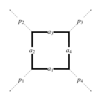
(a) (a)

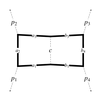
(b) (b)

Figure 1: Families of massive one- and two-loop integrals for light-by-light scattering. Possible irreducible numerator factors at two loops are not shown.

Let us introduce the integral families that we are going to discuss in this paper. As was already mentioned, the motivation for these particular integrals is that they can be used to study light-by-light scattering in planar $\mathcal{N}=4$ super Yang-Mills chpaper2 .

We define the inverse propagators

$$D_{1}(k)= -k^{2}+m^{2},\quad D_{3}(k)= -(k+p_{1}+p_{2})^{2}+m^{2},$$

$$D_{2}(k)= -(k+p_{1})^{2}+m^{2},\quad D_{4}(k)= -(k-p_{4})^{2}+m^{2}.$$ (4)

Note that we changed the convention for the metric w.r.t. Alday:2009zm to the mostly minus metric ($+-\ldots-$). The integrals we discuss include the one-loop family

$$G_{{a_{1},\ldots a_{4}}}= \int\frac{d^{D}k_{1}}{i\pi^{D/2}}\frac{1}{D_{1}(k_{1})^{a_{1}}D_{2}(k_{1})^{a_{2}}D_{3}(k_{1})^{a_{3}}D_{4}(k_{1})^{a_{4}}}\,,$$ (5)

where the $a_{i}$ can take any integer values. At two loops we discuss the family

$$G_{{a_{1},\ldots,a_{4}},{b_{1},\ldots,b_{4}},{c}}= \int\frac{d^{D}k_{1}d^{D}k_{2}}{(i\pi^{D/2})^{2}}\frac{D_{4}(k_{1})^{-a_{4}}}{D_{1}(k_{1})^{a_{1}}D_{2}(k_{1})^{a_{2}}D_{3}(k_{1})^{a_{3}}}$$

$$\times\,\frac{D_{2}(k_{2})^{-b_{2}}}{D_{1}(k_{2})^{b_{1}}D_{3}(k_{2})^{b_{3}}D_{4}(k_{2})^{b_{4}}}\frac{1}{[-(k_{1}-k_{2})^{2}]^{c}}\,,$$ (6)

where $a_{4}\leq 0,b_{2}\leq 0$ represent possible numerator factors. See Fig. 1(a) and Fig. 1(b) for the one- and two-loop cases, respectively. Finally, defining

$$G_{{a_{1},\ldots,a_{4}},{b_{1},\ldots,b_{4}},{c_{1},\ldots,c_{4}},{d,e,f}}= \int\frac{d^{D}k_{1}d^{D}k_{2}d^{D}k_{3}}{(i\pi^{D/2})^{3}}\frac{D_{1}(k_{1})^{-a_{1}}D_{4}(k_{1})^{-a_{4}}}{D_{2}(k_{1})^{a_{2}}D_{3}(k_{1})^{a_{3}}}\frac{D_{1}(k_{3})^{-c_{1}}D_{2}(k_{3})^{-c_{2}}}{D_{3}(k_{3})^{c_{3}}D_{4}(k_{3})^{c_{4}}}$$

$$\times\,\frac{D_{3}(k_{2})^{-b_{3}}}{D_{1}(k_{2})^{b_{1}}D_{2}(k_{2})^{b_{2}}D_{4}(k_{2})^{b_{4}}}\frac{1}{[-(k_{1}-k_{2})^{2}]^{d}[-(k_{2}-k_{3})^{2}]^{e}[-(k_{1}-k_{3})^{2}]^{f}}\,,$$ (7)

the two three-loop families we discuss are the following. For the first family, $a_{4}\leq 0,b_{2}\leq 0,b_{4}\leq 0,c_{2}\leq 0,f\leq 0$ represent possible numerator factors, and the second family is defined in the same way, but instead with $a_{1}\leq 0,a_{4}\leq 0,b_{3}\leq 0,c_{1}\leq 0,c_{2}\leq 0$. They are represented in Fig. 2(a) and Fig. 2(b), respectively.

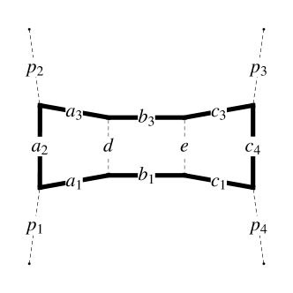
(a) (a)

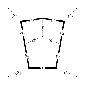
(b) (b)

Figure 2: Families of massive three-loop integrals for light-by-light scattering. Possible irreducible numerator factors are not shown.

Each $G$ is a function of the dimension $D$, the Mandelstam variables $s=(p_{1}+p_{2})^{2}$ and $t=(p_{2}+p_{3})^{2}$, and the internal mass $m$. The on-shell conditions for the external legs read $p_{i}^{2}=0$ for $i=1,2,3,4$.

A one-loop integral in the above family will be said to be dual conformal invariant, or DCI for short, if

$$a_{1}+a_{2}+a_{3}+a_{4}= 4\,.$$ (8)

The name is motivated by a natural generalization to a multiple mass case, where one can define dual conformal transformations under which the integral is covariant, see Alday:2009zm and the review Henn:2011xk . We use a similar definition at higher loops, equating to 4 the sum of indices associated with each loop variable. For example, a two-loop integral is DCI if $(a_{1}+a_{2}+a_{3}+a_{4}+c)=4$ and $(b_{1}+b_{2}+b_{3}+b_{4}+c)=4$.

In the following, we will define all integrals in the Euclidean region $s/m^{2}<0,t/m^{2}<0$, where all functions are real-valued. One then defines the functions elsewhere by analytic continuation, using the Feynman prescription. This implies giving the kinematical variables a small imaginary part, according to $m^{2}\rightarrow m^{2}-i0,s\rightarrow s+i0,t\rightarrow t+i0$.

Let us have a first look at these integrals, and take $I_{1}$ as an example. It is given analytically by (the form below is due to Davydychev:1993ut ),

$$I_{1}= \frac{2}{{\beta}_{uv}}\Big{\{}2\log^{2}\left(\frac{{\beta}_{uv}+{\beta}_{u}}{{\beta}_{uv}+{\beta}_{v}}\right)+\log\left(\frac{{\beta}_{uv}-{\beta}_{u}}{{\beta}_{uv}+{\beta}_{u}}\right)\log\left(\frac{{\beta}_{uv}-{\beta}_{v}}{{\beta}_{uv}+{\beta}_{v}}\right)-\frac{\pi^{2}}{2}$$

$$+\sum_{i=1,2}\Big{[}2\,{\rm Li}_{2}\left(\frac{\beta_{i}-1}{{\beta}_{uv}+\beta_{i}}\right)-2\,{\rm Li}_{2}\left(-\frac{{\beta}_{uv}-\beta_{i}}{\beta_{i}+1}\right)-\,\log^{2}\left(\frac{\beta_{i}+1}{{\beta}_{uv}+\beta_{i}}\right)\Big{]}\Big{\}}\,.$$ (9)

Here we introduced dimensionless variables

$$u=\frac{4m^{2}}{-s}\,,\qquad v=\frac{4m^{2}}{-t}\,,$$ (10)

and the following abbreviations,

$${\beta}_{u}=\sqrt{1+u}\,,\qquad{\beta}_{v}=\sqrt{1+v}\,,\qquad{\beta}_{uv}=\sqrt{1+u+v}\,.$$ (11)

The functions appearing in eq. (2) are examples of polylogarithms. For these and more general classes of integral functions that we will discuss one can define a “symbol” Goncharov:1998kja ; arXiv:math/0606419 ; Goncharov:2010jf . Roughly speaking, the symbol contains information about the integration kernels leading to those functions, while forgetting about boundary constants at each integration step. We note that the symbol of the above formula is very simple, and visibly more compact compared to eq. (2),

$${\mathcal{S}}\left[{\beta}_{uv}\,I_{1}\right]=2\left[\frac{{\beta}_{u}-1}{{\beta}_{u}+1}\otimes\frac{{\beta}_{uv}-{\beta}_{u}}{{\beta}_{uv}+{\beta}_{u}}+\frac{{\beta}_{v}-1}{{\beta}_{v}+1}\otimes\frac{{\beta}_{uv}-{\beta}_{v}}{{\beta}_{uv}+{\beta}_{v}}\right]\,.$$ (12)

This foreshadows a simple structure of the integral under the action of differential operators. In the next two sections, we will see how this structure arises in a systematic way. It will however not be necessary to restrict the analysis to the level of the symbol, rather the observations will apply to the functions directly. Indeed, we will be able to write compact formulas in terms of iterated integrals that make the simplicity manifest, while at the same time keeping track of the integration constants.

In particular, the complete information specifying the multi-loop integrals we will discuss will be contained in simple formulas similar to eq. (12). In the next two sections, we will first see how to reproduce this formula from differential equations, and then proceed to compute the required integrals at two and three loops.

3 Differential equation at one loop: $4$ versus $D$ dimensions

Computing loop integrals via differential equations is by now a fairly standard procedure Kotikov:1990kg ; Remiddi:1997ny ; Gehrmann:1999as ; Argeri:2007up , so we will only briefly outline the main steps. For a given class of integrals under consideration, defined by the propagator structure, one defines integral families for any possible powers of the propagators. E.g. at one loop, the family we consider is defined by eq. (5), see also Fig. 1(a), for any integer values of the parameters $a_{i}$. The integrals in a given family are in general not independent. They satisfy integration-by-parts (IBP) identities Chetyrkin:1981qh . The latter are linear in the integrals. In practice, this means that one can relate the calculation of any given integral to a finite number of master integrals. The algebraic manipulations needed are straightforward but cumbersome, so that one usually performs them using computer algebra codes. We have used FIRE Smirnov:2008iw ; Smirnov:2013dia , as well as an own implementation, to be described below. Other public computer codes include vonManteuffel:2012np ; Lee:2012cn . The independent integrals obtained in this way are usually referred to as master integrals. The basis choice is not unique. We have found Lee:2013hzt helpful to verify the number of master integrals needed in a given sector.

For a given set of master integrals, one sets up differential equations in the kinematical invariants. The derivative w.r.t. $m^{2}$ is straightforward to implement. The derivatives w.r.t. $s$ and $t$ can be written down via the chain rule, in terms of derivatives w.r.t. the external momenta, e.g.

$$\frac{\partial}{\partial s}=\frac{1}{2}\left[\frac{1}{s}p_{1}^{\mu}-\frac{2s+t}{s(s+t)}p_{2}^{\mu}+\frac{1}{s+t}p_{4}^{\mu}\right]\frac{\partial}{\partial p_{2}^{\mu}}\,.$$ (13)

When acting with the operator (13) on integrals such as (5), it is clear that the resulting terms will still be within the same family of integrals. Therefore, any derivative of a master integral can be expressed in terms of a linear combination of master integrals. This implies that the master integrals satisfy a linear system of first-order equations. Let us discuss this system in the one-loop case.

It is well known that the set of master integrals at one-loop, in the presence of internal masses, consists of the box, triangles, bubbles and tadpole topologies. Thanks to symmetries, for the present configuration this amounts to six master integrals. As we will see, the corresponding $6\times 6$ system of differential equations can be put in the form of eq. (1) by choosing the following basis of master integrals,

$$f_{1}= 2c\,m^{2}G_{{0,0,0,3}}$$ (14)

$$f_{2}= -\epsilon c\,\sqrt{s(s-4m^{2})}G_{{1,0,2,0}}$$

$$f_{3}= -\epsilon c\,\sqrt{t(t-4m^{2})}G_{{0,1,0,2}}$$

$$f_{4}= \epsilon^{2}c\,sG_{{1,1,1,0}}$$

$$f_{5}= \epsilon^{2}c\,tG_{{1,1,0,1}}$$

$$f_{6}= \frac{1}{2}\epsilon^{2}c\,\sqrt{st(st-4m^{2}(s+t))}G_{{1,1,1,1}}\,,$$

where $c=m^{2\epsilon}/\Gamma(1+\epsilon)$ is a convenient overall factor.

We start by setting up the system of first-order differential equations for the basis functions $f_{i}$. which takes the form, in our basis choice,

$$\partial_{s}\vec{f}=\epsilon\,\tilde{A}_{s}\vec{f}\qquad\partial_{t}\vec{f}=\epsilon\,\tilde{A}_{t}\vec{f}\,,\qquad\partial_{m^{2}}\vec{f}=\epsilon\,\tilde{A}_{m^{2}}\vec{f}\,.$$ (15)

The crucial simplification of our basis choice lies in the fact that the partial derivative matrices $\tilde{A}_{s},\tilde{A}_{t}$ and $\tilde{A}_{m^{2}}$ are independent of $\epsilon$. Moreover, as we will see presently, they can be expressed in terms of derivatives of logarithms only.

The $f_{i}$ are normalized to be dimensionless functions and therefore satisfy

$$(s\partial_{s}+t\partial_{t}+m^{2}\partial_{m^{2}})\vec{f}=0\,,$$ (16)

which is a useful consistency check. Other consistency checks are obtained from requiring that partial derivatives commute, which implies

$$[\tilde{A}_{i},\tilde{A}_{j}]=0\,,\qquad\partial_{i}\tilde{A}_{j}-\partial_{j}\tilde{A}_{i}=0\,,$$ (17)

where $i,j$ can be $s,t$, or $m^{2}$.

The structure of the differential equations, and hence that of the $f_{i}$, is greatly clarified by combining equations (15) by writing them in differential form

$$d\,\vec{f}=\epsilon\,(d\tilde{A})\,\vec{f}\,.$$ (18)

This is the form quoted in the introduction. Here $\tilde{A}$ was obtained by integrating the partial differential equations

$$\partial_{s}\tilde{A}=\tilde{A}_{s}\,,\qquad\partial_{t}\tilde{A}=\tilde{A}_{t}\,,\qquad\partial_{m^{2}}\tilde{A}=\tilde{A}_{m^{2}}\,.$$ (19)

This integration is very similar to the one that is needed to integrate $\vec{f}$ (at the first order in the $\epsilon$ expansion). Performing it at this stage allows us to completely elucidate the properties of the functions $\vec{f}$. In fact, we find that $\tilde{A}$ can be written in terms of logarithms only,

$$\tilde{A}= \left(\begin{array}[]{*{6}{c}}0&0&0&0&0&0\\ \cline{1-1}\cr\vrule\lx@intercol\hfil\log\left({\frac{{\beta}_{u}-1}{{\beta}_{u}+1}}\right)\hfil\lx@intercol\vrule\lx@intercol&\log{\frac{u}{1+u}}&0&0&0&0\\ \vrule\lx@intercol\hfil\log\left({\frac{{\beta}_{v}-1}{{\beta}_{v}+1}}\right)\hfil\lx@intercol\vrule\lx@intercol&0&\log{\frac{v}{1+v}}&0&0&0\\ \cline{1-1}\cr\cline{2-3}\cr 0&\vrule\lx@intercol\hfil-\log\left({\frac{{\beta}_{u}-1}{{\beta}_{u}+1}}\right)\hfil\lx@intercol&\lx@intercol\hfil 0\hfil\lx@intercol\vrule\lx@intercol&0&0&0\\ 0&\vrule\lx@intercol\hfil 0\hfil\lx@intercol&\lx@intercol\hfil-\log\left({\frac{{\beta}_{v}-1}{{\beta}_{v}+1}}\right)\hfil\lx@intercol\vrule\lx@intercol&0&0&0\\ 0&\vrule\lx@intercol\hfil\log\left({\frac{{\beta}_{uv}-{\beta}_{u}}{{\beta}_{uv}+{\beta}_{u}}}\right)\hfil\lx@intercol&\lx@intercol\hfil\log\left({\frac{{\beta}_{uv}-{\beta}_{v}}{{\beta}_{uv}+{\beta}_{v}}}\right)\hfil\lx@intercol\vrule\lx@intercol&\log\left({\frac{{\beta}_{uv}-1}{{\beta}_{uv}+1}}\right)&\log\left({\frac{{\beta}_{uv}-1}{{\beta}_{uv}+1}}\right)&\log\left({\frac{u+v}{1+u+v}}\right)\\ \cline{2-3}\cr\end{array}\right)\,.$$ (26)

We have ‘boxed’ the elements which survive in the $\epsilon\to 0$ limit, to be discussed presently.

To fully define the answer we need to specify a boundary condition. For the integrals under consideration a particularly natural boundary point is $m=\infty$, where

$$\vec{h}(\epsilon)\equiv\lim_{m\to\infty}\vec{f}(s,t,m^{2};\epsilon)=\delta_{i,1}\,.$$ (27)

Before commenting on the solution to the differential equations, let us first discuss a simplification for finite integrals.

We will be particularly interested in the $\epsilon\to 0$ limit. Since all the above integrals are both ultraviolet and infrared convergent (thanks to the internal masses, and thanks to the choice of representatives we made), it is natural to remove the powers of $\epsilon$ in eq. (14) in the limit. We thus let

$$(g_{1},g_{2},g_{3},\tilde{g}_{4},\tilde{g}_{5},g_{6})=\lim_{\epsilon\to 0}\,(f_{1},\frac{1}{\epsilon}f_{2},\frac{1}{\epsilon}f_{3},\frac{1}{\epsilon^{2}}f_{4},\frac{1}{\epsilon^{2}}f_{5},\frac{1}{\epsilon^{2}}f_{6}).$$ (28)

The powers of $\epsilon$ reflect the transcendental weights of the functions $g_{i}$. We have placed ‘tilde’ on $\tilde{g}_{4}$ and $\tilde{g}_{5}$ to distinguish them from two-loop integrals $g_{4}$ and $g_{5}$ which will be introduced in the next section. The integrals $g_{1},g_{2},g_{3}$ and $g_{6}$ will carry the same meaning throughout this paper.

The differential equation for the $g_{i}$ takes the similar canonical form (3), with the $A$-matrix obtained from $\tilde{A}$ in eq. (26) by retaining only the boxed elements.

Two observations will be important for us.

• The integrals $g_{i}$ have uniform transcendental weights $(0,1,1,2,2,2)$, respectively. This follows immediately from the block-triangular structure of the $A$-matrix: the derivatives of $g_{6}$ are expressed in terms of $g_{2},g_{3}$ only, while the derivatives of the latter are expressed in terms of $g_{1}$ only. Another way of seeing this is to note that the functions $f_{i}$ have uniform weight zero, and the rescaling by powers of $\epsilon$, which can be assigned weight $-1$, leads to the weight of the $g_{i}$ given above.

• The box $g_{6}$ and triangles $\tilde{g}_{4},\tilde{g}_{5}$ are fully decoupled in $D=4$.

The block triangular structure of the matrix and its implication for the weight of the functions is visualized in a different way in Fig. 3. There one can also see the decoupling of the box and triangle integrals.

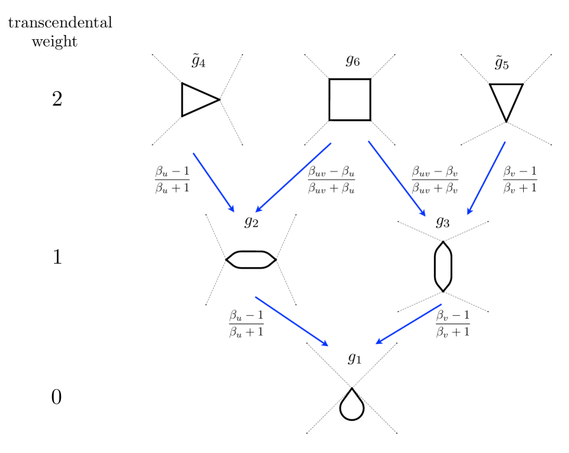
Figure 3: Hierarchy of one-loop functions. The integrals are classified according to their (transcendental) weight, shown in the leftmost column. Each arrow corresponds to one non-zero element of the derivative matrix $A$, cf. eq. (26). The fact that arrows only link integrals in adjacent rows is the statement that the matrix is block triangular. Solid and dashed lines denote massive and massless propagators, respectively.

The decoupling of the triangles implies that, if we are interested only in evaluating the box integral in $D=4$, we could consistently work with the truncated basis $g_{1},g_{2},g_{3}$ and $g_{6}$. Specifically, the system of differential equations in this case reduces to, cf. eq. (26),

$$d\left(\begin{array}[]{*{1}{c}}g_{1}\\ g_{2}\\ g_{3}\\ g_{6}\end{array}\right)= d\,\left(\begin{array}[]{*{4}{c}}0&0&0&0\\ \cline{1-1}\cr\vrule\lx@intercol\hfil\log\left({\frac{{\beta}_{u}-1}{{\beta}_{u}+1}}\right)\hfil\lx@intercol\vrule\lx@intercol&0&0&0\\ \vrule\lx@intercol\hfil\log\left({\frac{{\beta}_{v}-1}{{\beta}_{v}+1}}\right)\hfil\lx@intercol\vrule\lx@intercol&0&0&0\\ \cline{1-1}\cr\cline{2-3}\cr 0&\vrule\lx@intercol\hfil\log\left({\frac{{\beta}_{uv}-{\beta}_{u}}{{\beta}_{uv}+{\beta}_{u}}}\right)\hfil\lx@intercol&\lx@intercol\hfil\log\left({\frac{{\beta}_{uv}-{\beta}_{v}}{{\beta}_{uv}+{\beta}_{v}}}\right)\hfil\lx@intercol\vrule\lx@intercol&0\\ \cline{2-3}\cr\end{array}\right)\left(\begin{array}[]{*{1}{c}}g_{1}\\ g_{2}\\ g_{3}\\ g_{6}\end{array}\right)\,,$$ (41)

in agreement with the general form of eq. (3). Such truncations will be exploited extensively in the next section.

Let us now discuss the general solution in $D=4-2\epsilon$ dimensions, and then come back to the simplifications as $\epsilon\to 0$. With the differential equations in the form (18) we can immediately write down the analytic answer in terms of Chen iterated integrals Chen1997 . We have

$$\vec{f}(s,t,m^{2};\epsilon)={\mathbb{P}}e^{\epsilon\int_{{\gamma}}d\,\tilde{A}}\,\vec{h}(\epsilon)\,.$$ (42)

Here the integration contour ${\gamma}$ is a path in the space of kinematical variables, which begins at a base point, in our case $m\to\infty$, where we have the simple boundary condition (27).

Let us be more specific about the notation, following closely the recent lecture notes iterated1 ; iterated2 on iterated integrals. We denote by $\mathcal{M}$ the space of kinematical variables, here $(u,v)\in\mathbb{R}^{2}$, and let $\omega_{i}$ be some differential one-forms (corresponding to entries of $d\,\tilde{A}$ or $d\,A$). Moreover, define the pull-back of the differential forms to the unit interval $[0,1]$ via

$$\gamma^{*}(\omega_{i})=f_{i}(t)dt\,.$$ (43)

Then, an ordinary line integral is given by

$$\int_{\gamma}\omega_{1}=\int_{[0,1]}\gamma^{\star}(\omega_{1})=\int_{0}^{1}f_{1}(t_{1})t_{1}\,.$$ (44)

Then, the iterated integral of $\omega_{1},\ldots\omega_{n}$ along $\gamma$ is defined by

$$\int_{\gamma}\omega_{1}\ldots\omega_{n}=\int_{0\leq t_{1}\leq\ldots\leq t_{n}\leq 1}f_{1}(t_{1})dt_{1}\ldots f_{n}(t_{n})dt_{n}\,.$$ (45)

Iterated integrals have many nice properties, see iterated1 ; iterated2 . Moreover, the iterated integrals appearing in eq. (42) are homotopy invariant (on $\mathcal{M}$ with the set of singularities removed). This property makes them very flexible, and we will see later that how to rewrite them in terms of more familiar functions, if desired. We will also discuss expansions in limits and their numerical evaluation.

Expanding eq. (42) to second order in $\epsilon$ and noting that the box integral $I_{1}$ in eq. (2) is simply $\frac{1}{\epsilon^{2}}\frac{2}{{\beta}_{uv}}f_{6}$, it is trivial to reproduce its symbol given in eq. (12) starting from the $\tilde{A}$-matrix. With a little bit more work, it is also possible to verify that $I_{1}$ indeed obeys the claimed differential equation and boundary condition.

More generally, one may expand the solution to any desired order in $\epsilon$. With the normalization of the master integrals of eq. (14), the term multiplying $\epsilon^{k}$ will be a $\mathbb{Q}$-linear combination of $k$-fold iterated integrals, i.e. integrals of weight $k$. Such functions are sometimes called pure functions.

Let us now discuss the simplifications that occur for the four-dimensional basis (41). The solution can be again be written as in eq. (42), with the difference that $\epsilon$ is removed, and that only a finite number of terms have to be kept in the exponential.

The block diagonal form of $d\,A$ implies the particularly simple iterative structure of the integrals that we already alluded to earlier when discussing the symbol. The iterative solution starts with the weight zero function $1$, represented by the tadpole integral $g_{1}$. To obtain the weight one integrals, we simply have to follow the arrows shown in Fig. 3 back up (starting from the tadpole). To each arrow corresponds an element of the $d\,A$-matrix, and the contribution is given by the integral over the latter. For example,

$$g_{2}=\int_{{\gamma}}d\,\log\frac{{\beta}_{u}-1}{{\beta}_{u}+1}\,.$$ (46)

As was explained before, the integration is along a contour $\gamma$ in $(u,v)$ space, starting at the boundary point $u,v\to\infty$ corresponding to $m^{2}\to\infty$. Of course the above integral just evaluates to $\log\frac{{\beta}_{u}-1}{{\beta}_{u}+1}$, but this notion will be important when generalizing to higher weight functions. Next, the formulas for the weight two functions are obtained by summing over all paths from the tadpole to the integral under consideration. The contribution of each path is an iterated integral over the differential forms corresponding to each arrow. In this way, one arrives at

$$g_{6}=\int_{{\gamma}}d\,\log\frac{{\beta}_{u}-1}{{\beta}_{u}+1}\,d\log\frac{{\beta}_{uv}-{\beta}_{u}}{{\beta}_{uv}+{\beta}_{u}}+\int_{{\gamma}}d\,\log\frac{{\beta}_{v}-1}{{\beta}_{v}+1}\,d\,\log\frac{{\beta}_{uv}-{\beta}_{v}}{{\beta}_{uv}+{\beta}_{v}}\,.$$ (47)

Note that only the sum of the two iterated integrals in eq. (47) is homotopy invariant, not the individual terms. We can compare this to eq. (12), keeping in mind that $g_{6}=\lim_{\epsilon\to 0}\frac{\beta_{uv}}{2}I_{1}$. As was already mentioned, the difference is that, unlike the symbol, eq. (47) completely determines the answer.

We see that the solution is specified by the set of differential forms $\omega_{i}$ allowed to appear in the iterated integrals. This alphabet can be read off directly from the $d\,\tilde{A}$ or $d\,A$ matrices. Of course, for multivalued functions depending on many kinematical variables, one can expect this alphabet, which is related to possible singularities of the functions, to be relatively complicated. As we will see, one can often choose specific contours $\gamma$ that express the Chen iterated integrals in terms of more common multiple polylogarithms Goncharov:1998kja ; arXiv:math/0606419 , at the cost of giving up the homotopy invariance and the compactness of the expressions. An example is given in appendix C. The general formulas are also very useful for discussing analytic continuation and for studying simplifying limits, where again one often finds expressions in terms of multiple polylogarithms. Many examples can be found in chpaper2 . Discontinuities of the functions are also very transparent, see section 5.

In this section we have explained how to obtain a simplified version of the differential equations in the $\epsilon\to 0$ limit, starting from the $D=4-2\epsilon$ dimensional case. We saw that this implied that we could work with a smaller set of integrals which satisfy block-triangular systems of differential equations. In the next section, we will explain how to arrive at such results working directly in four dimensions.

4 Differential equation in $D=4$: two and three loops

In $D=4$ a natural subset of integrals to consider are the dual conformal ones, cf. eq (8). As we will see shortly, the derivatives of dual conformal integrals with respect to kinematic variables are themselves dual conformal. Therefore, one expects to be able to find a closed set of differential equations among dual conformal integrals. This has several advantages over the $D$-dimensional approach.

By restricting to a subset of integrals closed under differential equations, the number of integrals we need to consider in total decreases. This, and the possibility of setting $D=4$ from the start results in much faster computer implementations of the algebra needed to derive the differential equations. This allowed us to extend the analysis to the three-loop level.

In this section we describe the method. The first step, to generate tables of integration-by-part identities among dual conformal integrals, is discussed in subsection 4.1. An interesting feature of working in $D=4$ dimensions is that the identities sometimes contain contact terms, allowing different loop orders to be seamlessly merged. Once some basis of dual conformal master integrals has been found, our next step was to find a change of basis that puts the differential equation into the canonical block triangular form. It turns out that in $D=4$ this problem is much simpler compared to the $\epsilon\neq 0$ case, and can be solved systematically. We detail the procedure in subsection 4.2. We conclude this section with the main result for the two- and three-loop integrals.

4.1 Integration by part identities among dual conformal integrals

It is natural to expect that among all integration-by-parts identities, there exists a non-empty subset of identities, which hold exactly in $D=4$, and which relate only dual conformal integrals to one another. Identifying this subset starting from a list of $D$-dimensional reduction identities among non-conformal integrals might seem like a daunting task. It turns out that this admits a rather elegant solution in terms of the embedding formalism.

The embedding formalism is ideally suited to this problem, because writing a non-conformal expression in this formalism requires a deliberate effort. The main idea is to write propagators as linear functions of a $(D{+}2)$-vector $Y_{i}\simeq(k_{i}^{\mu},-k_{i}^{2},1)$, where the $Y_{i}$’s obey certain equivalence relations. The formalism is described in appendix B. As an example, the one-loop integral of eq. (5) is rewritten in the form

$$G_{{a_{1},\ldots,a_{4}}}=\int_{Y_{1}}\frac{(Y_{1}I)^{\sum_{i}a_{i}-D}}{(Y_{1}X_{1})^{a_{1}}(Y_{1}X_{2})^{a_{2}}(Y_{1}X_{3})^{a_{3}}(Y_{1}X_{4})^{a_{4}}}\,.$$

The numerator is necessary to ensure that the integrand has uniform homogeneity degree $D$ under rescaling of $Y_{1}$. The important feature here is that dual conformal integrals are precisely those for which the “point at infinity” $I$ is absent. By simply never introducing this point, one automatically stays within the class of conformal integrals.

Since the $(D{+}2)$-vectors $Y_{i}$ are a trivial change of variable away from the original loop momenta $k_{i}$, it is straightforward to carry through all the usual operations (generation of integration by parts identities, derivatives with respect to external variables, etc.) in terms of these variables. The upshot is that we automatically generate identities which involve only dual conformal integrals.

In order not to distract from the main course of this paper, these technical matters are discussed extensively in appendix B. Here we record only the most salient features in which $D=4$ differs from $D\neq 4$:

• Integration-by-part identities in $D=4$ sometimes contain contact terms, which appear through the identity (136)

  $$\frac{\partial}{\partial k_{1}^{\mu}}\frac{(k_{1}-k_{2})^{\mu}}{(k_{1}-k_{2})^{4}}=2\pi^{2}i\delta^{4}(k_{1}-k_{2})\,.$$

  This identity effectively relates integrals with different loop orders, since the $\delta$-function removes one integration variable.

• When working without a regulator it is important to restrict attention to convergent integrals, which converge in all integration regions. To this aim we imposed a simple set of sufficient conditions on the set of integrals we have considered, also listed in appendix B.

• Derivatives of dual conformal integrals with respect to kinematic variables are themselves dual conformal, see e.g. eq. (141).

By generating identities among dual-conformal integrals in $D=4$ and following standard integral reduction algorithms, we have reduced all integrals which appearing in derivatives to a minimal basis. Before we describe this basis, it is convenient to perform a certain basis change.

4.2 Algorithm for obtaining the differential in canonical form

Perhaps the most striking feature of working in $D=4$ is that the $A$ matrix, in a suitable basis, is expected to admit a block-triangular form. This reflects the existence of master integrals which have uniform transcendental weights. Assuming that such a basis exists, a constructive algorithm can find it!

The method is actually rather straightforward: first we put the system into triangular form, by finding the proper normalization of (suitable combinations of) the master integrals. This already introduces a first approximation to the notion of weight. Then we recursively shift integrals by lower weight ones, until all differentials can be written in “d-$\log$” form; the matrix will then automatically be block-triangular.

We explain the three steps of our method, illustrating them with simple examples.

Step 1. Obtaining a triangular form.

We decompose the integrals into two sets: correctly “normalised” and “remaining” ones. We assume that the constant integral ($g_{1}$) is part of the basis; by definition it is correctly normalised. We then successively normalise the remaining integrals as follows.

First we find the smallest subset of remaining integrals, whose derivatives involve only themselves and normalised ones. As a trivial example, in the two-loop case after we had normalised the integrals $g_{1},g_{2},g_{3},g_{4}$ (see below for their definitions), the smallest subset consisted of just one element:

$$\frac{d}{ds}G_{{0,1,2,0},{2,0,1,0},{1}}= -2\frac{s-3m^{2}}{s(s-4m^{2})}G_{{0,1,2,0},{2,0,1,0},{1}}\,\,({\rm mod}\,g_{1},g_{2},g_{3},g_{4}).$$ (48)

We integrate this equation, working modulo already normalised integrals:

$$\frac{d}{ds}\left(sm^{2}\sqrt{s(s-4m^{2})}G_{{0,1,2,0},{2,0,1,0},{1}}\right)= 0\,\,({\rm mod}\,g_{1},g_{2},g_{3},g_{4}).$$ (49)

Since the right-hand side involves only other, already normalised integrals, we declare the parenthesis to be correctly normalised and we add it to the list. We then repeat the same procedure for the remaining integrals.

Sometimes the smallest closed set of remaining integrals contains more than one element. This happened to us at three loops; for example at some point we had the “entangled” pair of integrals

$$\quad\vec{h}= \big{(}G_{{0,1,2,0},{2,0,0,0},{2,0,1,0},{1,1,0}},G_{{0,2,1,0},{2,0,0,0},{2,0,1,0},{1,1,0}}\big{)}$$

with the differential equation

$$\frac{d}{ds}\vec{h}= \vec{h}M\,\,({\rm mod\,normalised}),\qquad M=\frac{m^{4}}{s}\left(\begin{array}[]{c@{\,\,\,\,}c}\frac{2}{4m^{2}-s}&-2\\ \frac{10}{4m^{2}-s}&-4\end{array}\right).$$ (52)

The right-hand side can be removed by considering the ansatz $I=\vec{h}.(c_{1},c_{2})$ and solving the differential equation $\frac{d}{ds}(c_{1},c_{2})=-M(c_{1},c_{2})$. The solution gives that

$$\frac{d}{ds}\left(\begin{array}[]{l}s^{2}\left[(4m^{2}-s)(2m^{2}-s)h_{1}+(10m^{4}-10m^{2}s+s^{2})h_{2}\right]\\ s\sqrt{s(s-4m^{2})}\left[(2m^{4}-4m^{2}s+s^{2})h_{1}+(2m^{4}-6m^{2}s+2s^{2})h_{2}\right]\end{array}\right)= 0\quad({\rm mod\,normalised}).$$ (55)

These two combinations can now be added to the list of normalised integrals, and the procedure repeated for the next subset. It is noteworthy that even at three loops we never had to integrate anything more complicated than a $2\times 2$ matrix.

This procedure successfully puts the differential equation into strict triangular form, which is already a tremendous simplification. We stress the critical role of $D=4$ for this to be possible (see for example appendix A for a discussion of the $D\neq 4$ case). The integrals do not, yet, however, have uniform transcendental weight.

Step 2. Obtaining a block-triangular form.

We start from the triangular form of the differential equation and again split the integrals into two sets, “UT” (for uniform transcendental degree, or weight) and “remaining” ones. The UT integrals are assigned definite weights. At the beginning only the constant integral $g_{1}$ is UT, and its weight is defined to be 0.

We pick one of the remaining integrals whose derivatives involve only integrals in the UT set. Such integrals always exist, since the system is already strictly triangular. We must figure out the weight of that integral. To do this we integrate the coefficients of the maximal weight UT integrals on the right-hand-side of the differential equation and ask whether they contain transcendental parts or not. If they do, the weight of the integral will be one more than the weight on the right-hand side. If they do not, we remove the highest weight on the right-hand-side by a judicious redefinition, and repeat.

Let us illustrate this with a simple example. After $g_{1},g_{2},g_{3},g_{4}$ were put in UT form, we had the equation

$$\frac{d}{ds}\left(sm^{2}\sqrt{s(s-4m^{2})}G_{{0,1,2,0},{2,0,1,0},{1}}\right)= \frac{-4m^{4}g_{4}+2m^{2}sg_{1}}{s\sqrt{s(s-4m^{2})}}+\frac{8m^{4}g_{2}}{s(s-4m^{2})}.$$ (56)

The presence of $g_{4}$ on the right-hand side, which has weight 2, would suggest that the parenthesis has weight 3. However, when we integrate the coefficient of $g_{4}$, we find that it contains no logarithm:

$$\int ds\frac{-4m^{4}}{s\sqrt{s(s-4m^{2})}}=2m^{2}\sqrt{(s-4m^{2})/s}+c_{1},$$ (57)

where $c_{1}$ is an ($s$-independent) integration constant. This shows that $g_{4}$ can be removed by a simple redefinition of the integral. After we do this, we are led to integrate the coefficient of $g_{2}$, which is now the highest weight integral on the right-hand side (it has weight 1). This time we find that its primitive contains a logarithm: this cannot be removed by a simple redefinition. Including an integration constant for $g_{2}$, and setting $c_{1}=0$ since there is no use for it anymore (the integral under consideration turned out to have the same weight as $g_{4}$), we now have

$$\frac{d}{ds} \left[sm^{2}\sqrt{s(s-4m^{2})}G_{{0,1,2,0},{2,0,1,0},{1}}-2m^{2}\sqrt{(s-4m^{2})/s}\,g_{4}+c_{2}g_{2}\right]$$ (58)

$$=2g_{2}\left[\frac{d}{ds}\log(s-4m^{2})\right]+(4+2c_{2})g_{1}\left[\frac{d}{ds}\log\big{(}\sqrt{-s}+\sqrt{4m^{2}-s}\big{)}\right]\,.$$

Finally we set $c_{2}=-2$ to remove the last term, which would have the wrong weight. The parenthesis is now a UT integral of weight 2, one more than the weight of $g_{2}$. We add it to the list and repeat the procedure for the next integral.

The general procedure is as follows. Once we have identified the weight of the integral, we have two tasks: i) we must remove non-logarithmic terms in the highest-weight part of the derivatives ii) we must remove all terms involving lower-weight integrals (such as $g_{1}$ in the example). Both of these tasks are carried out order by order in decreasing weight. Non-logarithmic terms at high weights are removed by shifting the definition of the integral (like we did for $g_{4}$ above), while at lower weights it is also necessary to adjust integration constants from the previous weight. We believe that this procedure will always successfully find a UT basis if it exists.

Step 3. Optimizing the solution.

The UT master integrals generated by the above procedure can be quite lengthy and far from optimal. This is especially so for the highest weight UT integrals, which can end up expressed as combinations of all the other integrals in the original basis.

The good news is that once some UT basis has been found, it is very easy to find other, more compact, ones.

Returning to the example in eq. (58), it is natural to consider other candidate master integrals for the same topology:

$$G_{{0,1,2,0},{2,0,1,0},{1}}\,,\quad G_{{0,2,1,0},{2,0,1,0},{1}}\,,\quad G_{{0,1,2,0},{1,0,2,0},{1}}\quad\mbox{and}\quad G_{{0,2,1,0},{1,0,2,0},{1}}\,.$$

By construction, each of these may be reduced to linear combinations of UT master integrals. One can then search, among these integrals, for combinations which reduce directly to the parenthesis in eq. (58). That way we found the rather compact combination recorded as $g_{5}$ in eq. (59) below.

Contrary to the previous steps, there is of course no systematic procedure for finding “the nicest possible” representative. In most cases, we could find satisfactory combinations by trying a rather obvious set of candidates.

4.3 Result at two and three loops: UT basis and differential equation

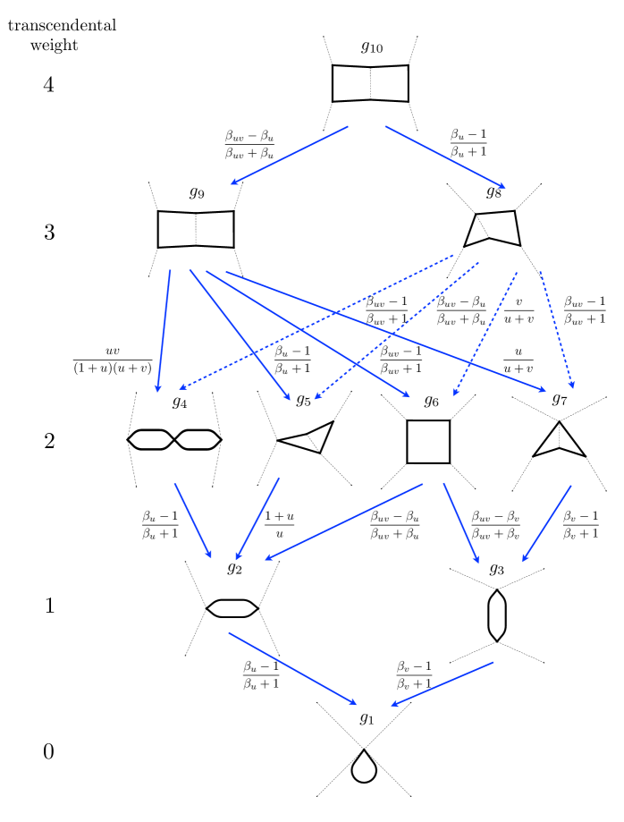
Figure 4: Hierarchy of master integrals up to two loops. The integrals are classified according to their (transcendental) weight, shown in the leftmost column. Each arrow corresponds to one non-zero element of the derivative matrix $A$, cf. eq. (72). The fact that arrows only link integrals in adjacent rows is the statement that the matrix is block triangular. The result for an integral can immediately be written down by summing over all paths leading up from the tadpole integral $g_{1}=1$. Each path gives a contribution to an iterated integral, with the integration kernels being specified by the ‘letters’ written next to the corresponding arrows. Solid and dashed lines denote massive and massless propagators, respectively. Note that the pictures are intended to give an idea of how the integrals look like, but omit details such as e.g. numerator factors.

The complete basis of four-dimensional DCI integrals for the family (2) is given as follows. First we have the four one-loop integrals

$$g_{1}= 6m^{4}G_{{4,0,0,0}}$$ (59)

$$g_{2}= -\frac{1}{2}\sqrt{s(s-4m^{2})}\left[(2m^{2}-s)G_{{2,0,2,0}}+4m^{2}G_{{1,0,3,0}}\right]$$

$$g_{3}= -\frac{1}{2}\sqrt{t(t-4m^{2})}\left[(2m^{2}-t)G_{{0,2,0,2}}+4m^{2}G_{{0,1,0,3}}\right]$$

$$g_{6}= \frac{1}{2}\sqrt{st(st-4m^{2}(s+t))}G_{{1,1,1,1}}\,.$$

These integrals are equal to the corresponding ones defined in eq. (14), but the present form makes the dual conformal symmetry manifest. In addition we have the two-loop integrals

$$g_{4}= \frac{1}{2}(g_{2})^{2}$$ (60)

$$g_{5}= \frac{1}{2}sm^{2}\sqrt{s(s-4m^{2})}\left[G_{{0,1,2,0},{2,0,1,0},{1}}+G_{{0,2,1,0},{2,0,1,0},{1}}\right]$$

$$g_{7}= -tm^{4}\left[G_{{0,1,2,0},{0,0,2,1},{1}}+2G_{{0,2,1,0},{0,0,1,2},{1}}+3G_{{0,1,2,0},{0,0,1,2},{1}}\right]$$

$$g_{8}= -\frac{1}{2}m^{2}\sqrt{st(st-4m^{2}(s+t))}\left[G_{{0,1,2,0},{1,0,1,1},{1}}+G_{{0,2,1,0},{1,0,1,1},{1}}\right]$$

$$g_{9}= -\frac{1}{4}sm^{2}\left[sG_{{1,1,1,0},{1,-1,1,2},{1}}+2tG_{{1,1,1,0},{0,0,1,2},{1}}\right]$$

$$g_{10}= \frac{1}{8}\sqrt{s(s-4m^{2})}\sqrt{st(st-4m^{2}(s+t))}G_{{1,1,1,0},{1,0,1,1},{1}}\,.$$

All integrals are convergent. It is easy to see that they obey the boundary condition

$$\lim_{m\to\infty}g_{i}=\delta_{i,1}.$$ (61)

They obey the differential equation in the canonical form (3), with the $A$-matrix

$$A= \left(\begin{array}[]{cccccccccc}0&0&0&0&0&0&0&0&0&0\\ \cline{1-1}\cr\vrule\lx@intercol\hfil{\frac{{\beta}_{u}-1}{{\beta}_{u}+1}}\hfil\lx@intercol\vrule\lx@intercol&0&0&0&0&0&0&0&0&0\\ \vrule\lx@intercol\hfil{\frac{{\beta}_{v}-1}{{\beta}_{v}+1}}\hfil\lx@intercol\vrule\lx@intercol&0&0&0&0&0&0&0&0&0\\ \cline{1-3}\cr 0&\vrule\lx@intercol\hfil{{\frac{{\beta}_{u}-1}{{\beta}_{u}+1}}}\hfil\lx@intercol&\lx@intercol\hfil{0}\hfil\lx@intercol\vrule\lx@intercol&0&0&0&0&0&0&0\\ 0&\vrule\lx@intercol\hfil{{\frac{1+u}{u}}}\hfil\lx@intercol&\lx@intercol\hfil{0}\hfil\lx@intercol\vrule\lx@intercol&0&0&0&0&0&0&0\\ 0&\vrule\lx@intercol\hfil{{\frac{{\beta}_{uv}-{\beta}_{u}}{{\beta}_{uv}+{\beta}_{u}}}}\hfil\lx@intercol&\lx@intercol\hfil{{\frac{{\beta}_{uv}-{\beta}_{v}}{{\beta}_{uv}+{\beta}_{v}}}}\hfil\lx@intercol\vrule\lx@intercol&0&0&0&0&0&0&0\\ 0&\vrule\lx@intercol\hfil{0}\hfil\lx@intercol&\lx@intercol\hfil{{\frac{{\beta}_{v}-1}{{\beta}_{v}+1}}}\hfil\lx@intercol\vrule\lx@intercol&0&0&0&0&0&0&0\\ \cline{2-7}\cr 0&0&0&\vrule\lx@intercol\hfil{{\frac{{\beta}_{uv}-1}{{\beta}_{uv}+1}}}\hfil\lx@intercol&{\frac{{\beta}_{uv}-{\beta}_{u}}{{\beta}_{uv}+{\beta}_{u}}}&{\frac{v}{u+v}}&\lx@intercol\hfil{{\frac{{\beta}_{uv}-1}{{\beta}_{uv}+1}}}\hfil\lx@intercol\vrule\lx@intercol&0&0&0\\ 0&0&0&\vrule\lx@intercol\hfil{{\frac{uv}{(1+u)(u+v)}}}\hfil\lx@intercol&{\frac{{\beta}_{u}-1}{{\beta}_{u}+1}}&{\frac{{\beta}_{uv}-1}{{\beta}_{uv}+1}}&\lx@intercol\hfil{{\frac{u}{u+v}}}\hfil\lx@intercol\vrule\lx@intercol&0&0&0\\ \cline{4-9}\cr 0&0&0&0&0&0&0&\vrule\lx@intercol\hfil{{\frac{{\beta}_{u}-1}{{\beta}_{u}+1}}}\hfil\lx@intercol&\lx@intercol\hfil{{\frac{{\beta}_{uv}-{\beta}_{u}}{{\beta}_{uv}+{\beta}_{u}}}}\hfil\lx@intercol\vrule\lx@intercol&0\\ \cline{8-9}\cr\end{array}\right)\,.$$ (72)

We have abbreviated each nonzero entry of the matrix by omitting the logarithm; for example $A_{2,1}\equiv\log{\frac{{\beta}_{u}-1}{{\beta}_{u}+1}}$.

The differential equation (3), with the $A$-matrix (72) and boundary condition (61), completely determines the integral. The block-triangular nature of the matrix, highlighted by its presentation, reflects the uniform transcendental weights of the integrals. The weights can be read off from the matrix structure: $g_{1}$; $g_{2,3}$; $g_{4,5,6,7}$; $g_{8,9}$ and $g_{10}$ have uniform weights 0,1,2,3 and 4.

As in the preceding section, the differential equation admits a natural graphical representation, see Fig. 4. The solution to the differential equation can be read off directly from this figure, as was explained in section 3.

4.4 Numerical evaluation

We would like to stress that, for practical purposes, Fig. 4 contains all relevant information about the double box integral.

Consider, for example, its numerical evaluation. As discussed in the end of section 3, each path between $g_{10}$ and $g_{1}$ translates to an iterated integral:

$$g_{10}(u,v)= \int_{0}^{1}\partial_{t_{4}}\log\frac{{\beta}_{u}(t_{4})-1}{{\beta}_{u}(t_{4})+1}\,\,\partial_{t_{3}}\log\frac{{\beta}_{uv}(t_{3})-1}{{\beta}_{uv}(t_{3})+1}\,\,\partial_{t_{2}}\log\frac{{\beta}_{v}(t_{2})-1}{{\beta}_{v}(t_{2})+1}\,\,\partial_{t_{1}}\log\frac{{\beta}_{v}(t_{1})-1}{{\beta}_{v}(t_{1})+1}$$

$$+\mbox{9 other terms.}$$ (73)

The integration variables are ordered: $1{>}t_{4}{>}t_{3}{>}t_{2}{>}t_{1}{>}0$. The shown term corresponds to the rightmost path in Fig. 4. In the end $g_{10}$ is independent of the choice of path going to $(u,v)$ starting from infinity, but one simple choice is $(u(t),v(t))=(u/t,v/t)$, $t\in[0,1]$. There are in total 10 paths in the figure, and the sum of the 10 associated terms represents $g_{10}$ exactly. Alternatively, the 10 terms can be generated by solving formally the differential equation $dg_{i}=(dA)_{ij}g_{j}$, with the $A$-matrix given in eq. (72) and boundary condition $\lim_{u,v\to\infty}g_{i}=\delta_{i1}$.

Although it can be evaluated numerically, the four-fold integral (73) is obviously not optimal. Many integrals can be done analytically. For example, the $t_{1}$ and $t_{4}$ integrations obviously only produce logarithms, so at most two integrations really need to be done numerically. In fact, since analytic expressions for the weight 2 functions $g_{4,5,6,7}$ are easy to obtain, the $t_{2}$ integration can be also done analytically. In this way Fig. 4 immediately produces a one-fold integral representation for the double box:

$$g_{10}(u,v)= \int_{0}^{1}dt\,\log\frac{({\beta}_{uv}-{\beta}_{u})({\beta}_{uv}(t)+{\beta}_{u}(t))}{({\beta}_{uv}+{\beta}_{u})({\beta}_{uv}(t)-{\beta}_{u}(t))}\left[g_{4}(u)\frac{d}{dt}\log\left(\frac{uv}{(1+u)(u+v)}\right)\right.$$

$$\hskip 14.22636pt\left.+g_{5}(u)\frac{d}{dt}\log\left(\frac{{\beta}_{u}-1}{{\beta}_{u}+1}\right)+g_{6}(u,v)\frac{d}{dt}\log\left(\frac{{\beta}_{uv}-1}{{\beta}_{uv}+1}\right)+g_{7}(v)\frac{d}{dt}\log\left(\frac{u}{u+v}\right)\right]$$

$$\!\!\!\!\!+\int_{0}^{1}dt\,\log\frac{({\beta}_{u}-1)({\beta}_{u}(t)+1)}{({\beta}_{u}+1)({\beta}_{u}(t)-1)}\left[g_{4}(u)\frac{d}{dt}\log\left(\frac{{\beta}_{uv}-1}{{\beta}_{uv}+1}\right)\right.$$

$$\hskip 14.22636pt\left.+g_{5}(u)\frac{d}{dt}\log\left(\frac{{\beta}_{uv}-{\beta}_{u}}{{\beta}_{uv}+{\beta}_{u}}\right)+g_{6}(u,v)\frac{d}{dt}\log\left(\frac{v}{u+v}\right)+g_{7}(v)\frac{d}{dt}\log\left(\frac{{\beta}_{uv}-1}{{\beta}_{uv}+1}\right)\right]\,,$$ (74)

where everything in the square brackets is evaluated at $(u(t),v(t))$. In addition to $g_{6}=\frac{{\beta}_{uv}}{2}I_{1}$ which was given previously in eq. (2), the functions are ($x\equiv\frac{{\beta}_{u}-1}{{\beta}_{u}+1}$):

$$g_{4}(u)=\frac{1}{2}(\log x)^{2}\,,\qquad\quad g_{5}(u)=2{\rm Li}_{2}(-x)+2\log x\log(1+x)-\frac{1}{2}(\log x)^{2}+\zeta_{2}\,,$$ (75)

and $g_{7}=g_{4}(v)$. We found the representation (74) to be very well suited for numerical evaluation, with the number of digits of accuracy increasing linearly with computing time (when implemented in Mathematica).

It is also possible to convert Fig. 4 automatically into expressions involving Goncharov polylogarithms. This exploits a judicious parametrization of the kinematic variables, as discussed in appendix C. These can then be evaluated numerically, using, for example Bauer:2000cp ; Vollinga:2004sn . In practice, we found the representation (74) to be both more direct to implement, easier to analytically continue and generally faster.

Before closing this section, we wish to emphasize that Fig. 4 is also a useful starting point for expanding the integrals in various kinematical limits. Often, the alphabet simplifies in these cases, and a representation in terms of simpler standard functions can be given. For example, let us consider the Regge limit, $s\rightarrow\infty$, $t$ fixed. Choosing the parametrization $-t/m^{2}=x/(1-x)^{2}$ for convenience, after a little algebra one sees that the alphabet required for all functions including the three-loop ones simplifies to

$$\{x\,,1+x\,,1-x\}\,.$$ (76)

This implies that the Regge expansion of all integrals, to any order in $1/s$, can be given in terms of powers of $s$ and $\log s$, multiplied by harmonic polylogarithms Remiddi:1999ew of argument $x$. Such expansions, as well as their physical interpretation, will be discussed in greater detail in ref. chpaper2 .

4.5 Result at three loops

A remarkable feature of the preceding computation is the surprisingly small amount of CPU power and memory usage that it required, as well as the fact that all manipulations are essentially algorithmic and with little need for trial-and-error. Furthermore the final form of the differential equation is pleasingly compact. These findings encouraged us to go to three loops. Indeed, the algorithms described above carried seamlessly through the three-loop integrals of the considered family, if only that more CPU power was required, as detailed in appendix B.

For the two families in Fig. 2 combined (and including all one- and two- loop sub-topologies), our final result for the UT basis contains 48 master integrals, 38 of them being relevant to the computation of the three-loop light-by-light amplitude chpaper2 (i.e. the remaining 10 integrals decouple from the problem). In particular, the triple ladder integral, and the ‘tennis court’ integral with a single numerator are part of our basis,

$$g_{37}= -\frac{1}{16}(4m^{2}-s)s\sqrt{st(-4sm^{2}-4tm^{2}+st)}\,G_{{1,1,1,0},{1,0,1,0},{1,0,1,1},{1,1,0}}\,,$$ (77)

$$g_{38}= -\frac{1}{8}\sqrt{-(4m^{2}-t)t}\sqrt{st(-4sm^{2}-4tm^{2}+st)}G_{{0,1,1,0},{1,1,-1,1},{0,0,1,1},{1,1,1}}\,.$$ (78)

The system of differential equation, which takes a hierarchical form as found previously at one- and two- loops, is given for the 38 first integrals in appendix D. The full system, including the definitions of all the integrals in the basis, is attached as an ancillary file with the arXiv submission of this article. As before, this results contains all the information needed for efficient numerical evaluation of the integrals, the study of their limits, analytic continuation, etc. Here we simply note that the alphabet at three loops is not the same as at two loops. In addition to the entries in eq. (72) and their $u\leftrightarrow v$ symmetric values, the $A$-matrix, and hence the alphabet, contains the new entries

$$dA\supset\left\{d\log\left(u^{2}-4v\right)\,,d\log\left(v^{2}-4u\right)\,,d\log\left(\frac{2-2\beta_{uv}+u}{2+2\beta_{uv}+u}\right)\,,d\log\left(\frac{2-2\beta_{uv}+v}{2+2\beta_{uv}+v}\right)\right\}$$ (79)

These new letters reveal the existence of a new scale in the problem, $s\sim t^{2}/m^{2}$, where the three-loop amplitude exhibits nontrivial features. While the physical significance of this scale remains to be clarified, this suggests that other scales (and other letters) will continue to appear at each loop oder.

5 Analyticity properties and Mandelstam representation

The differential equation can be most readily integrated in the Euclidean region $u,v>0$, but this is not the only region of physical interest. To carry out their analytic continuation to other regions, it is important to know where the singularities lie.

A useful way to encode the analytic properties of an amplitude is through dispersive-type representations. The one-loop box integral (2) is known to admit the following remarkable integral representation Mandelstam:1959bc ; Davydychev:1993ut

$$M^{(1)}(u,v)= -2\int_{\Delta(\xi,\eta)}\frac{d\xi d\eta}{(\xi+u)(\eta+v)\sqrt{1-\xi-\eta}}\,.$$ (80)

The integration region is the triangle $\Delta(\xi,\eta)=\{\xi,\eta:\xi\geq 0,\eta\geq 0,\xi+\eta\leq 1\}$. This representation makes the analyticity properties of the integral in the complex $u$ and $v$ planes completely manifest, because all the singularities originate from the denominator. The integral is therefore analytic for $(u,v)\in(\mathbb{C}\backslash[-1,0])^{2}$. Furthermore the discontinuity with respect to $u$ enjoys analytic properties with respect to $v$.

Representations of this type are known as Mandelstam representations, following an early proposal by Mandelstam Mandelstam:1958xc . To our knowledge, the existence of the Mandelstam representation has never been conclusively proved nor disproved, not even to all orders in perturbation theory. There is a known perturbative obstruction at one-loop, namely the presence of so-called anomalous thresholds. These are singular branch points that are unrelated to the physical thresholds $s,t=4m^{2}$ and which occur when the internal and external masses in a problem violate certain inequalities. In the equal mass case this obstruction is absent, in agreement indeed with the existence of the formula (80). Mandelstam proposed that if such a representation exists at one-loop for a given process, it should continue to exist at all loop orders for this process. We can test this hypothesis using the obtained differential equation.

We checked the analyticity properties of the integrals as follows. Starting from the point $u,v=\infty$, we integrate the differential equation along $u$ with $v=\infty$. We find a single branch cut along $u\in[-1,0]$, as expected (in this interval $s>4m^{2}$) and we evaluate the discontinuity across it. (In fact the $u$ dependence at $v=\infty$ can be expressed analytically in terms of harmonic polylogarithms, similarly to the Regge limit as discussed around eq. (76), so at this stage everything is analytic.) We then integrate the discontinuity along the $v$ direction, keeping $u$ fixed. Although the differential equation has in principle many loci of singularity, we find (numerically) for all integrals in our three-loop basis only two branch points, located at $v=0$ and $v=-1-u$, indicating that the other singularities are spurious. This implies that all integrals, in our two- and three-loop families, possess the analyticity properties implied by the Mandelstam representation.

We should note that, for these statements to be true, it is important to consider integrals with rational coefficients, e.g. we have to divide the $g_{i}$’s in eq. (59) by the square roots which appear in their normalization. Computing the discontinuity of the discontinuity, for $v\in[-1-u,0]$, constructively produces the integrand of the Mandelstam representation. Up to two loops we obtained closed-form analytic formulae:

$$g_{6}(u,v)= {\beta}_{uv}\int_{\Delta(\xi,\eta)}\frac{d\xi d\eta}{(\xi+u)(\eta+v)\sqrt{1-\xi-\eta}}$$ (81)

$$g_{8}(u,v)= {\beta}_{uv}\int_{\Delta(\xi,\eta)}\frac{d\xi d\eta}{(\xi+u)(\eta+v)\sqrt{1-\xi-\eta}}\log\left(\frac{\eta}{\xi+\eta}\right)$$

$$g_{9}(u,v)= \int_{\Delta(\xi,\eta)}\frac{d\xi d\eta}{(\xi+u)(\eta+v)}\log\left(\frac{1-\sqrt{1-\xi-\eta}}{1+\sqrt{1-\xi-\eta}}\right)$$

$$+\int_{0}^{1}\frac{d\xi}{\xi+u}\left(4{\rm Li}_{2}(\xi)+2\log\xi\log(1-\xi)-\frac{\pi^{2}}{6}\right)$$

$$g_{10}(u,v)= {\beta}_{u}{\beta}_{uv}\int_{\Delta(\xi,\eta)}\frac{d\xi d\eta\,h_{10}(-\xi,-\eta)}{(\xi+u)(\eta+v)\sqrt{1-\xi}\sqrt{1-\xi-\eta}}$$

where

$$h_{10}(u,v)= {\rm Li}_{2}\left(\frac{{\beta}_{uv}+{\beta}_{u}}{{\beta}_{uv}+1}\right)+{\rm Li}_{2}\left(\frac{{\beta}_{uv}-{\beta}_{u}}{{\beta}_{uv}-1}\right)-{\rm Li}_{2}\left(\frac{{\beta}_{uv}+{\beta}_{u}}{{\beta}_{uv}-1}\right)-{\rm Li}_{2}\left(\frac{{\beta}_{uv}-{\beta}_{u}}{{\beta}_{uv}+1}\right)$$

$$+\log\left(\frac{1+{\beta}_{u}}{1-{\beta}_{u}}\right)\log\left(\frac{u+v}{v}\right)-\frac{\pi^{2}}{2}.$$

All of these integrals are manifestly analytic in the cut complex plane $(u,v)\in(\mathbb{C}\backslash[-1,0])^{2}$. The square roots ${\beta}_{u},{\beta}_{uv}$ factored out in front of the integrals are precisely those which appear in the corresponding normalization factors in eq. (59), as just mentioned.

The remaining integrals in our two-loop basis depend on only one variable at a time and admit the more familiar single-variable dispersion relations:

$$g_{2}(u)= -{\beta}_{u}\int_{0}^{1}\frac{d\xi}{(\xi+u)\sqrt{1-\xi}}$$ (82)

$$g_{4}(u)= \int_{0}^{1}\frac{d\xi}{(\xi+u)}\log\left(\frac{1+\sqrt{1-\xi})}{1-\sqrt{1-\xi}}\right)$$

$$g_{5}(u)= {\beta}_{u}\int_{0}^{1}\frac{d\xi}{(\xi+u)\sqrt{1-\xi}}\log\left(\frac{\xi}{4(1-\xi)}\right)\,.$$

Also $g_{1}=1$, $g_{3}=g_{2}(v)$ and $g_{7}=g_{4}(v)$.

The analyticity properties which we have verified for the three-loop integrals imply that they also admit Mandelstam representations, but we did not study these explicitly.

These dispersion relations can be written in a more familiar form using the change of variable $u=4m^{2}/(-s)$, $\xi=4m^{2}/s^{\prime}$:

$$\int_{0}^{1}\frac{d\xi}{\xi+u+i0}F(\xi)=\int_{4m^{2}}^{\infty}\frac{s\,ds^{\prime}}{s^{\prime}(s-s^{\prime}-i0)}F\left(\frac{4m^{2}}{s^{\prime}}\right)\,.$$ (83)

Here we have included Feynman’s $i0$ prescription, implicit in all preceding equations, but required to make sense of the integral when $s>4m^{2}$ or $t>4m^{2}$. We recognize the right-hand-side as a once-subtracted dispersion relation. The subtraction constants happen to vanish for all integrals in eqs. (82), because the left-hand-sides vanish at $s=0$. Similar comments apply to the Mandelstam representations (81), where the one subtraction for $g_{9}$ is due to its nonvanishing value at $t=0$.

We mention that at an early stage of this work, we actually successfully guessed an analytic expression for the two-loop integral $g_{10}$, by simply assuming that it admitted a Mandelstam representation! The reason is that its integrand (i.e. the function $h_{10}$ above) has only transcendental weight 2, so by assuming that all entries of its symbol are taken from the finite alphabet $(u,v,{\beta}_{u},{\beta}_{v},{\beta}_{u}+1,{\beta}_{v}+1,{\beta}_{uv}+1,{\beta}_{u}+{\beta}_{uv},{\beta}_{v}+{\beta}_{uv})$ as suggested by the one-loop computation, one arrives at a relatively compact ansatz. We could then fix all coefficients using reality considerations, symmetries, Regge limits, and numerical evaluation at one point. However, we must warn the reader that such a procedure is far from systematic. At three loops our ansatz would most likely have missed the new entries of the symbol shown in eq. (79), and would thus have led us to a wrong answer, if any. The differential equation approach in contrast is completely systematic and reliable.

6 Checks

We have performed a number of checks on our calculations. First of all, there are many internal consistency checks for the differential equations, for example the integrability conditions (17) for the matrices appearing in different partial derivatives.

Moreover, as discussed in appendix A, the integrals we computed contain simpler two-scale form-factor type integrals that were previously computed Anastasiou:2006hc . We have performed tests against the results given in that reference. Our results also include (a subset of) two-loop integrals occurring in top quark pair production cross sections Czakon:2008ii . They can be obtained from our formulas by taking an $s$- or $t$-channel discontinuity and going to certain forward limits. In particular, in this way we checked that the singularity structure of the integrals shown in Fig. 4(b)-(d) of the above reference can be understood by taking forward limits of the alphabet we found here in the general kinematical case. Moreover, we have done a detailed check for the cut double box integral shown in Fig. 4(b) of that reference, which corresponds to ${\rm Disc}_{v}\left[g_{10}\right](u,-u)$, up to a normalization factor. Perhaps the easiest check can be done using the Mandelstam representation discussed in section 5, cf. eq. (81), which gives

$${\rm Disc}_{v}\left[g_{10}\right](u,-u)={\beta}_{u}\int_{0}^{1-u}d\xi\frac{\,h_{10}(-\xi,-u)}{(\xi+u)(\eta+v)\sqrt{1-\xi}\sqrt{1-\xi-u}}\,.$$ (84)

In this way, we numerically verified the result of Czakon:2008ii for that integral. It is also possible to give an analytic answer for this (and other) integrals, starting from the Chen iterated integral representation. In eq. (142) we give a convenient parametrization of $u$ and $v$ for rewriting those integrals in terms of multiple polylogarithms. Here it will suffice to remark that by specializing to the $v=-u$ case gives $u=4z(1-z^{2})/(1+z^{2})^{2}$, in which case the alphabet relevant for ${\rm Disc}_{v}\left[g_{10}\right](u,-u)$ reduces to $z,1\pm z,1+z^{2}$, i.e. a particularly simple case. Our results can also be used to derive similar formulas for other integrals in the same limit $v\mapsto-u$, including the three-loop ones, albeit using a larger alphabet.

Very strong tests were also provided by expansions of the integrals in various physical limits that will be discussed in detail in ref. chpaper2 . For example, we have successfully reproduced the known Regge limit of the three-loop ladder and tennis court integrals $g_{37}$ and $g_{38}$. Because of the iterative structure of the solution, this also tests to some extent the whole system of differential equations.

Finally we have performed numerical tests. The iterative structure of the differential equation allows for a simple numerical evaluation, as detailed in section 4.4. In the three-loop case, by working out analytic expressions for all weight 3 $g_{i}$ functions in terms of ${\rm Li}_{3}$ functions, and for the $t_{5},t_{6}$ integrals in terms of dilogarithms, we actually succeeded in obtaining a one-fold integral representation similar to eq. (74), which also converge rather fast. We then performed numerical comparisons against values obtained from FIESTA Smirnov:2008py ; Smirnov:2013eza . While it is difficult to estimate the expected error of multidimensional integration routines, based on gradually increasing the number of sampling points and observing stable results, we arrived at the following values and error estimates

$$g^{\rm FIESTA}_{10}(4,4)= \phantom{-}0.0528808\pm 0.0001\,,$$ (85)

$$g^{\rm FIESTA}_{37}(2,4)= \phantom{-}0.0764993\pm 0.0001\,,$$ (86)

$$g^{\rm FIESTA}_{38}(2,4)= -0.195813\pm 0.001\,.$$ (87)

Indeed, they perfectly agree to that precision with the results obtained from our analytic answer,

$$g_{10}(4,4)= \phantom{-}0.0530386297835364296406023741052\ldots$$ (88)

$$g_{37}(2,4)= \phantom{-}0.0764922717271986970254859257468\ldots$$ (89)

$$g_{38}(2,4)= -0.195801160078160255184758547581\ldots$$ (90)

We have also performed successful checks at other kinematical points, and for other integrals.

7 Conclusions

We have shown in this paper how to implement the differential equations method Kotikov:1990kg ; Remiddi:1997ny ; Gehrmann:1999as ; Argeri:2007up for a closed subset of finite (and dual conformal) integrals. The restriction to $D=4$ turns out to be a significant simplification of the method of ref. Henn:2013pwa , which was originally developed for arbitrary $D$ dimensions.

We expect that our approach can also be applied for other classes of convergent four-dimensional integrals, such as for example position space correlation functions. For instance, in ${\cal N}=4$ super Yang-Mills, expressions for the integrands of four-point correlation functions are known to relatively high loop order Eden:2012tu , and our method could be used to shed light on their functional dependence and to evaluate them analytically. Currently, the planar integrals up to three loops are known Drummond:2013nda . Another set of finite and dual conformal functions that this method could be applied to are ratio and remainder functions in ${\cal N}=4$ super Yang-Mills Drummond:2008vq .. Using a suitable four-dimensional regulator, such as for example differential renormalization Freedman:1991tk ; Gracia-Bondia:2014zwa , it seems reasonable to anticipate applicability of the method to correlation functions in an arbitrary quantum field theory.

It is important to stress that this approach to calculating integrals is systematic. We find it extremely satisfying that the algorithm developed in section 4 for the two-loop problem worked without any modification at three loops. However we do not have a proof that the algorithm will always succeed, and it will be interesting to try it on other problems, and also maybe generalize it to the $D$-dimensional case.

Our final result for the double box in $D=4$ reveals a simple iterative structure, summarized in Fig. 4. In fact the figure contains all needed information about the integral! For example, it can be evaluated numerically almost directly, as explained in section 4.4. It also provides an efficient starting point for expanding around various kinematic limits, as will be pursued in a companion paper chpaper2 . Finally, it can be automatically converted to a sum of standard special functions, for example Goncharov polylogarithms, as shown in appendix C. It is tempting to call Fig. 4 the answer for the double-box; it is the most concise and useful presentation which we can imagine on this day. The similar figure at three-loops is given in matrix form in appendix D.

It is tempting to expect such an iterative structure of the differential equation to be a general feature of Feynman integrals in integer dimensions. We expect this regardless of whether or not the integrals are expressible in terms of polylogarithm-type functions. For example, a similar iterative structure is also seen for integrals involving elliptic-type functions (see, for example, section 5 of Bloch:2013tra ).

We comment that the method automatically finds the ‘alphabet’ relevant to a problem. This is important since the alphabet may change from one loop order to the next. The three-loop octagon Wilson loops of ref. Caron-Huot:2013vda are a case in point; this paper provides another example, where the letters (79) would likely have been very difficult to guess. The alphabet specifies the class of two-variable functions describing the problem. Although the latter are rather complicated, we have demonstrated in this paper that they can be easily dealt with. In particular, we have shown how to evaluate them numerically, and discussed their analytic structure.

In addition to the expressions for all dual conformal invariant master integrals up to three loops, we have performed a complete calculation in dimensional regularization of the planar two-loop master integrals. The results, given in appendix A, can be used in future studies of light-by-light scattering at NLO, keeping the exact mass dependence. For previous studies in various mass regimes, see refs. Bern:2001dg ; Binoth:2002xg .

The integrals we computed may also be helpful for tackling problems on the 2013 Les Houches QCD wishlist, in particular when one wants to keep the exact dependence on quark masses. Indeed, the three-loop family we computed contain several integrals relevant for $gg\to H$ at NNNLO. Moreover, the process $gg\to gH$ at NNLO involves four-point functions similar to the ones computed here, albeit with one additional mass scale.

Appendix A Two-loop master integrals in $D$ dimensions from differential equations

Here we report on the computation of all master integrals of the integral family (2), see Fig. 1(b), in $D$ dimensions. Contrary to the main text, in this appendix we keep the full dependence on $\epsilon$. These integrals may be used in future applications for light-by-light scattering in QED or QCD, and we also hope that they provide a first useful step towards similar but more complicated integrals needed e.g. for $gg\to Hg$ at NNLO.

A.1 Choice of integral basis

We apply the method of differential equations as explained in the main text. Using the methods of ref. Henn:2013pwa , we arrived at the following convenient basis choice,

$$f_{1}= \,cG_{2,0,0,0,2,0,0,0,0}\,,$$ (91)

$$f_{2}= c\sqrt{s\left(s-4m^{2}\right)}G_{2,0,1,0,2,0,0,0,0}\,,$$ (92)

$$f_{3}= cs\left(4m^{2}-s\right)G_{2,0,1,0,2,0,1,0,0}\,,$$ (93)

$$f_{4}= -2c\epsilon sG_{2,0,0,0,1,0,1,1,0}\,,$$ (94)

$$f_{5}= c2\epsilon s\sqrt{s\left(s-4m^{2}\right)}G_{2,0,1,0,1,0,1,1,0}\,,$$ (95)

$$f_{6}= csG_{2,0,0,0,0,0,2,0,1}\,,$$ (96)

$$f_{7}= c\frac{1}{2}\sqrt{s\left(s-4m^{2}\right)}\left[2G_{2,0,0,0,0,0,1,0,2}+G_{2,0,0,0,0,0,2,0,1}\right]\,,$$ (97)

$$f_{8}= cm^{2}sG_{3,0,0,0,0,0,1,1,1}\,,$$ (98)

$$f_{9}= cm^{2}sG_{1,0,1,0,0,0,0,3,1}\,,$$ (99)

$$f_{10}= c(-2){\epsilon}sG_{1,0,1,0,0,0,0,2,1}\,,$$ (100)

$$f_{11}= c\sqrt{s\left(s-4m^{2}\right)}[m^{2}\left(G_{1,0,1,0,0,0,0,3,1}+G_{2,0,1,0,0,0,0,2,1}\right)-\frac{3}{2}{\epsilon}G_{1,0,1,0,0,0,0,2,1}]\,,$$ (101)

$$f_{12}= 4c{\epsilon}^{2}sG_{1,0,1,0,0,0,1,1,1}\,,$$ (102)

$$f_{13}= -4c{\epsilon}^{2}s\sqrt{s\left(s-4m^{2}\right)}G_{1,0,1,0,1,0,1,1,1}\,,$$ (103)

$$f_{14}= tcG_{0,2,0,0,0,0,0,2,1}\,,$$ (104)

$$f_{15}= c\frac{1}{2}\sqrt{t\left(t-4m^{2}\right)}\left[2G_{0,2,0,0,0,0,0,1,2}+G_{0,2,0,0,0,0,0,2,1}\right]\,,$$ (105)

$$f_{16}= cm^{2}tG_{1,1,0,0,0,0,0,3,1}\,,$$ (106)

$$f_{17}= 4c{\epsilon}^{2}tG_{1,1,0,0,1,0,0,1,1}\,,$$ (107)

$$f_{18}= -2c{\epsilon}\sqrt{s\left(m^{4}s-2m^{2}t(s+2t)+st^{2}\right)}G_{1,1,1,0,0,0,0,2,1}\,,$$ (108)

$$f_{19}= c\sqrt{st\left(st-4m^{2}(s+t)\right)}\left[m^{2}G_{1,1,1,0,0,0,0,3,1}-{\epsilon}G_{1,1,1,0,0,0,0,2,1}\right]\,,$$ (109)

$$f_{20}= -2c{\epsilon}s\left[G_{1,1,1,-1,0,0,0,2,1}-m^{2}G_{1,1,1,0,0,0,0,2,1}\right]\,,$$ (110)

$$f_{21}= 4c{\epsilon}^{2}(s+t)G_{0,1,1,0,1,0,0,1,1}\,,$$ (111)

$$f_{22}= -2c{\epsilon}\sqrt{st\left(st-4m^{2}(s+t)\right)}G_{0,1,1,0,1,0,0,1,2}\,,$$ (112)

$$f_{23}= -2c{\epsilon}m^{2}(s+t)\left[G_{0,1,2,0,1,0,0,1,1}+G_{0,2,1,0,1,0,0,1,1}\right]\,,$$ (113)

$$f_{24}= 4c{\epsilon}^{2}s^{2}G_{1,1,1,0,1,0,1,1,0}\,,$$ (114)

$$f_{25}= 4c{\epsilon}^{2}\left[sG_{1,1,0,0,1,-1,1,1,1}+tG_{0,1,1,0,1,0,0,1,1}\right]\,,$$ (115)

$$f_{26}= 4c{\epsilon}^{2}\sqrt{st\left(st-4m^{2}(s+t)\right)}G_{1,1,0,0,1,0,1,1,1}\,,$$ (116)

$$f_{27}= 4c{\epsilon}^{2}s\sqrt{t\left(s-4m^{2}\right)\left(st-4m^{2}(s+t)\right)}G_{1,1,1,0,1,0,1,1,1}\,,$$ (117)

$$f_{28}= -4c{\epsilon}^{2}\sqrt{s\left(s-4m^{2}\right)}\left[sG_{1,1,1,0,1,-1,1,1,1}+2tG_{1,1,0,0,1,0,1,1,1}\right]\,,$$ (118)

$$f_{29}= 4c\epsilon^{2}s\Big{[}-G_{1,0,1,0,1,0,1,0,1}+sG_{1,0,1,0,1,0,1,1,1}-2G_{1,1,0,0,1,-1,1,1,1}-2tG_{1,1,0,0,1,0,1,1,1}$$

$$\quad\quad+G_{1,1,1,-1,1,-1,1,1,1}-sG_{1,1,1,0,1,-1,1,1,1}+tG_{1,1,1,0,1,0,1,1,0}\Big{]}\,.$$ (119)

where the normalization factor $c$ is

$$c=1/\Gamma^{2}(1+\epsilon)\,e^{2\epsilon\gamma_{E}}\,\epsilon^{2}\,(m^{2})^{2\epsilon}\,.$$ (120)

The basis integrals are depicted (qualitatively) in Fig. 5. Integrals $f_{1}$ to $f_{13}$ are $s$-channel triangle integrals, while the subsequent four integrals are $t$-channel triangle integrals. These integrals were computed previously, to some order in $\epsilon$, in ref. Anastasiou:2006hc . The form of the basis we have chosen has the advantage that all basis elements have uniform weight and therefore are simpler compared to that reference. Some related integrals were also considered in ref. puhlfuerst .

We wish to comment that, contrary to the $D=4$ case, where we could employ the systematic algorithm presented in section 4, in the $D$-dimensional case finding the basis where 1 is satisfied required a fair amount of intuition, and trial and error. Also, the resulting $\tilde{A}$-matrix is no long block-triangular (nor even triangular).

(a) $f_{1}$

(b) $f_{14},f_{15}$

(c) $f_{6},f_{7}$

(d) $f_{2}$

(e) $f_{8}$

(f) $f_{4}$

(g) $f_{9},f_{10}$

(h) $f_{3}$

(i) $f_{16}$

(j) $f_{21},f_{22},f_{23}$

(k) $f_{12}$

(l) $f_{5}$

(m) $f_{17}$

(n) $f_{18},f_{19},f_{20}$

(o) $f_{13}$

(p) $f_{25},f_{26}$

(q) $f_{24}$

(r) $f_{27},f_{28},f_{29}$

Figure 5: Master integrals the integral family, organized by the number of propagators. Each integral stands for a set of integrals sharing the same propagators, with possible numerator factors not shown in the pictures.

A.2 Differential equations and analytic solution

With the above basis choice, we find the differential equations in the form of eq. (18), with $\tilde{A}$ being a $29\times 29$ matrix. It is given in electronic form as an ancillary file with the arXiv submission of this paper. As was discussed in the main text, the differential equations can be immediately solved, to any order in $\epsilon$, in terms of Chen iterated integrals, cf. eq. (42). The relevant boundary condition is

$$f_{i}(s=0,t=0;m^{2})=\delta_{i,1}\,.$$ (121)

The alphabet, i.e. the set of entries of the matrix appearing in the differential equations turns out to be given by

$$\{1+u+v\,,\frac{4-v+\beta}{4-v-\beta}\,,\frac{4+v+\beta}{4+v-\beta}\,,\frac{(4\beta_{u}+\beta)(4\beta_{u}+\beta_{u}v+\beta)}{(4\beta_{u}-\beta)(4\beta_{u}+\beta_{u}v-\beta)}\,,\frac{(4\beta_{uv}+\beta)(4\beta_{uv}-\beta_{uv}v+\beta)}{(4\beta_{uv}-\beta)(4\beta_{uv}-\beta_{uv}v-\beta)}\,,$$ (122)

with a new square root,

$$\beta=\sqrt{16+16u+8v+v^{2}}\,.$$ (123)

in addition to the letters present in (72). We see that the full $D$-dimensional solution has a more complicated structure than just the four-dimensional dual conformal integrals.

Remarkably, we find that the only new singularity introduced by (122) w.r.t. the four-dimensional case is $1+u+v=0$.

Appendix B Generation of IBP identities using the embedding formalism

Here we describe the generation of integration-by-parts identities among dual conformal integrals. We first briefly review the embedding formalism for arbitrary integrals in $D$-dimensions, following closely ref. SimmonsDuffin:2012uy , and then we set $D=4$ and restrict to conformal integrals.

B.1 Loop integrals in the embedding formalism

To each point $x^{\mu}$ in $D$-dimensional spacetime we assign a $(D{+}2)$-dimensional vector $X^{a}$ defined up to rescaling:

$$X^{a}=\left(\begin{array}[]{c}X^{\mu}\\ X^{-}\\ X^{+}\end{array}\right)\equiv\left(\begin{array}[]{c}x^{\mu}\\ -x^{2}\\ 1\end{array}\right)\,,\quad\mbox{with}\quad X^{a}\simeq\alpha X^{a}\quad(\alpha\neq 0)\,.$$ (124)

The projective identification naturally removes one degree of freedom from the $(D+2)$-vector $X$. The second degree of freedom is removed by the fact that the vector (124) is null with respect to the $(D+2)$-dimensional metric

$$(XY)\equiv 2X_{\mu}X^{\mu}+X^{+}Y^{-}+X^{-}Y^{+}\,.$$ (125)

Thus eq. (124) defines a one-to-one map between null projective $(D{+}2)$-vectors and points in (compactified) $D$-dimensional spacetime. Furthermore, the dot product of the representative (124) evaluates to $(XY)=-(x-y)^{2}$, effectively linearizing the propagators.

To handle massive propagators in momentum space, we relax the null condition and modify $X^{-}$ in eq. (124) such that $X^{2}=m^{2}$. As a concrete example, the inverse propagators defined in eq. (4) map to the following $(D{+}2)$-vectors:

$$X_{1}=\left(\begin{array}[]{c}0^{\mu}\\ m^{2}\\ 1\end{array}\right)\,,\qquad X_{2}=\left(\begin{array}[]{c}-p_{1}^{\mu}\\ m^{2}\\ 1\end{array}\right)\,,\qquad X_{3}=\left(\begin{array}[]{c}-(p_{1}+p_{2})^{\mu}\\ -s+m^{2}\\ 1\end{array}\right)\,,\qquad X_{4}=\left(\begin{array}[]{c}p_{4}^{\mu}\\ m^{2}\\ 1\end{array}\right)\,.$$ (126)

To make formulas invariant under choices of representative (124), it is useful to introduce an additional “infinity point”

$$I\equiv\left(\begin{array}[]{c}0^{\mu}\\ 1\\ 0\end{array}\right)\,.$$ (127)

Assigning the vector $Y_{1}\propto(k_{1}^{\mu},-k_{1}^{2},1)$ to the loop integration variable, in this notation we have

$$\frac{1}{D_{1}(k_{1})D_{2}(k_{1})D_{3}(k_{1})D_{4}(k_{1})}=\frac{(Y_{1}I)^{4}}{(Y_{1}X_{1})(Y_{1}X_{2})(Y_{1}X_{3})(Y_{1}X_{4})}\,.$$ (128)

All propagator factors are now linear in the integration variable $Y_{1}$.

The quadratic nature of the propagators has effectively been transferred to the integration measure: the $(D+2)$-vector $Y_{1}$ is to be integrated over the null cone $Y_{1}^{2}=0$, subject to the GL(1) “gauge symmetry” $Y_{1}\simeq\alpha Y_{1}$. A natural integration measure for this space is

$$\int_{Y_{1}}\equiv\int\frac{d^{D+2}Y_{1}\delta(\frac{1}{2}Y_{1}^{2})}{i\pi^{D/2}{\rm vol(GL(1))}}\,.$$ (129)

Here the notation $1/{\rm vol(GL(1))}$ means to insert appropriate gauge-fixing factors and Faddeev-Popov determinant, which should integrate to unity over each GL(1) gauge orbit. The notation is borrowed from ref. ArkaniHamed:2010gh .

A particularly simple gauge choice is $1/{\rm vol(GL(1))}\mapsto\delta((YI)-1)$; the Faddeev-Popov determinant is then unity. The general solution to the $\delta$-function constraint in this gauge takes the form (124), and in this gauge it is easy to see that the above measure is proportional to the usual one:

$$\int_{Y}\frac{1}{(YI)^{D}}=\int\frac{d^{D}k}{i\pi^{D/2}}$$ (130)

The left-hand-side is manifestly gauge-invariant (the GL(1) weight of the denominator cancels that of the measure in eq. (129)), so the identity does not depend on the gauge choice. For example we could gauge-fix using $1/{\rm vol(GL(1))}\mapsto\delta(((Y),I^{\prime})-1)$ for any $I^{\prime}$, and although the identity would be more difficult to see, it would still be true since it is clear that nothing can depend on $I^{\prime}$.

Combining the ingredients (128) and (130) we can write the integrals in our one-loop family as

$$G_{{a_{1},\ldots,a_{4}}}=\int_{Y_{1}}\frac{(Y_{1}I)^{2\epsilon+\sum_{i}a_{i}-4}}{(Y_{1}X_{1})^{a_{1}}(Y_{1}X_{2})^{a_{2}}(Y_{1}X_{3})^{a_{3}}(Y_{1}X_{4})^{a_{4}}}\,.$$ (131)

The special simplification in the conformal case $\epsilon=0$ and $\sum_{i}a_{i}=4$ is manifest: the dependence on $I$ drops out.

Generalization to higher loop planar integrals is straightforward: internal propagators become, for example, $1/(Y_{1}Y_{2})$. This will be sufficient for our purposes. It is unclear whether the formalism could be used for non-planar momentum space integrals, although we note that non-planar coordinate-space integrals would pose no problem.

B.2 Integration by parts identities: one-loop case

To derive integration-by-parts identities within the embedding formalism, we start from the usual fundamental identity Chetyrkin:1981qh ,

$$0=\int\frac{d^{D+2}Y}{{\rm vol(GL(1))}}\frac{\partial}{\partial Y^{a}}\delta(\frac{1}{2}Y^{2})V^{a}(Y)\,.$$ (132)

This expression makes sense (e.g. is invariant under the GL(1) gauge symmetry) provided that the vector is homogeneous: $V^{i}(Y)=\alpha^{D-1}V^{i}(\alpha Y)$. We stress that the derivative does not need to act on the gauge fixing factor “$1/{\rm vol(GL(1))}$” for this identity to be true.

To avoid taking derivatives of $\delta(\frac{1}{2}Y^{2})$, however, which would have no interpretations in terms of Feynman integrals, one must require orthogonality: $Y_{i}V^{i}(Y)=0$. This is trivially solved by $V^{a}\propto Y^{a}$, but, due to the homogeneity property, the right-hand-side of (132) can be seen to become zero trivially in this case, so one obtains no useful identity in this case. We conclude that $V^{a}(Y)$ is a homogeneous $(D{+}2)$-vector orthogonal to $Y^{a}$ and defined modulo $Y^{a}$. This effectively reduces its number of vector components to $D$, as expected. This agrees with other treatments of vector fields in the embedding formalism, see Weinberg:2010fx ; Costa:2011mg and references therein.

Let us now illustrate the rules with a simple example, involving a one-loop bubble:

$$0= \int_{Y}\frac{\partial}{\partial Y^{a}}Y_{b}\frac{X_{1}^{a}X_{3}^{b}-X_{1}^{b}X_{3}^{a}}{(YX_{1})(YX_{2})(YI)^{2-2\epsilon}}$$

$$= (4m^{2}-s)G_{{2,0,1,0}}+2(1-\epsilon)\big{(}G_{{1,0,1,0}}-G_{{2,0,0,0}}\big{)}-4m^{2}G_{{3,0,0,0}}\,.$$ (133)

The left-hand side is an allowed IBP vector because the replacement $\partial/\partial Y^{a}\mapsto Y_{a}$ yields zero, as required. This justifies our omission of the explicit $\delta(\frac{1}{2}Y^{2})$ factor, part of the definition of the measure (129). The right-hand side (in which we have used the symmetry $G_{{a_{1},a_{2},a_{3},a_{4}}}=G_{{a_{3},a_{2},a_{1},a_{4}}}$) can be easily verified to be indeed a valid integral identity.

To illustrate nontrivial identities among conformal integrals, we consider the triangle integrals:

$$0 =\int_{Y}\frac{\partial}{\partial Y^{i}}Y_{j}\frac{X_{1}^{i}X_{3}^{j}-X_{1}^{j}X_{3}^{j}}{(YX_{1})(YX_{2})(YX_{3})^{2}}=2m^{2}G_{{2,1,1,0}}+2m^{2}G_{{1,2,1,0}}+(2m^{2}-s)G_{{1,1,2,0}}+\ldots$$

$$0 =\int_{Y}\frac{\partial}{\partial Y^{i}}Y_{j}\frac{X_{2}^{i}X_{3}^{j}-X_{2}^{j}X_{3}^{j}}{(YX_{1})(YX_{2})(YX_{3})^{2}}=2m^{2}G_{{2,1,1,0}}+2m^{2}G_{{1,2,1,0}}+2m^{2}G_{{1,1,2,0}}+\ldots$$ (134)

where we have set $\epsilon=0$, and suppressed bubble and tadpole topologies from the right-hand-sides. One can see that combining these identities allows the triangles to be removed. Further reducing the bubbles, one obtains in this way the following reductions:

$$G_{{1,1,2,0}}=\frac{g_{2}-g_{1}}{s}=G_{{2,1,1,0}},\qquad G_{{1,2,1,0}}=\frac{(s-4m^{2})g_{2}+4m^{2}g_{1}}{2s}\,,$$ (135)

where the master integrals $g_{1}$ and $g_{2}$, defined in eq. (59), have at most two propagators. These identities, which hold only when $D=4$, explain the absence of conformal triangle integrals in the four-dimensional basis, cf. eq. (14).

B.3 Integration by parts identities: multi-loop case

The procedure we have just described generalizes trivially to the multi-loop case. However, new subtleties arise in the limit $D\to 4$.

The first subtlety is that we must carefully avoid divergent integrals. Ultraviolet convergence is already guaranteed for dual conformal integrals, to which we will restrict our attention when discussing $D=4$. Infrared divergences, however, could appear as a result of squaring the (massless!) internal propagators.

It is important to stress that, when working without a regulator, one should consider only integrals which are not only finite but convergent, e.g. separately finite in each integration region ArkaniHamed:2010gh ; Weinzierl:2014iaa .

As a simple sufficient condition for convergence, we have imposed the following constraints on the integrals in our basis:

• At two-loops, we require the internal propagator to occur with at most two powers, $1/(Y_{1}Y_{2})^{2}$. Squared internal propagators, when they appear, must multiply numerators which vanish when $Y_{1}=Y_{2}$.

• At three-loops, we impose the preceding conditions separately for each internal propagator. Convergence in the region $Y_{1}\to Y_{2}\to Y_{3}$ is then ensured by requiring that no more than one squared propagators appears.

These conditions define a restricted set of integrals, within which one can safely operate without regulator in $D=4$.

A second subtlety when $D=4$ is related to contact terms. These appear through the familiar identity

$$\frac{\partial}{\partial k_{1}^{\mu}}\frac{(k_{1}-k_{2})^{\mu}}{(k_{1}-k_{2})^{4}}=2\pi^{2}i\delta^{4}(k_{1}-k_{2})\,,$$ (136)

which holds when $D$ is exactly equal to four. As a simple way to derive the corresponding identity in the embedding formalism, we may the following result for logarithmically divergent divergent integrals:

$$\int_{Y_{1},Y_{2}}\frac{1}{(Y_{1}Y_{2})^{2}}F(Y_{1},Y_{2})=-\frac{1}{\epsilon}\int_{Y}F(Y,Y)+\mbox{finite}\,.$$ (137)

Imagine, now, that we have an IBP vector that contains a squared internal propagator (but with a numerator such that it generates only convergent conformal integrals when $D=4$). When we evaluate the IBP identity for $\epsilon\neq 0$, we get all the terms we get naively from $D=4$, plus some $\epsilon$-dependent terms. Actually the only $\epsilon$ dependence in the formalism comes from the derivative acting on $(Y,I)^{2\epsilon}$, producing

$$\int_{Y_{1},Y_{2}}\left(\frac{\partial}{\partial Y_{1}^{a}}(Y_{1}I)^{2\epsilon}\right)\frac{(Y_{2}I)^{2\epsilon}}{(Y_{1}Y_{2})^{2}}V^{(4)a}(Y_{1},Y_{2})=2\epsilon\int_{Y_{1},Y_{2}}\frac{(Y_{1}I)^{2\epsilon}(Y_{2}I)^{2\epsilon}}{(Y_{1}I)(Y_{1}Y_{2})^{2}}(I,V^{(4)}(Y_{1},Y_{2}))$$

$$=\left.-\frac{2\epsilon}{\epsilon}\int_{Y}\frac{(IV^{(4)}(Y,Y))}{(IY)}\right|_{D=4}+\mathcal{O}(\epsilon)\,.$$ (138)

We notice the $\epsilon/\epsilon$ cancelation, which means that this term survives the $\epsilon\to 0$ limit. This additional term can be interpreted as a contact term as in eq. (136):

$$\frac{\partial}{\partial Y_{1}^{a}}\frac{1}{(Y_{1}Y_{2})^{2}}V^{(4)a}(Y_{1},Y_{2})=-2\delta^{4}(Y_{1},Y_{2})\frac{(IV^{(4)}(Y,Y))}{(IY)}+\mbox{regular terms}\,,$$ (139)

where the $\delta$-function is normalized according to the measure (130): $\int_{Y}\delta^{4}(Y,Y^{\prime})F(Y)=F(Y^{\prime})$. The “regular terms” are all those obtained by the naive differentiation procedure in $D=4$.

The presence of the infinity point in this formula is surprising at first sight, but it has a simple interpretation. To see this, we can consider, as an alternative to dimensional regularization, regulating (132) by excising a small neighborhood of $Y_{1}=Y_{2}$. The contact term will then arise as a boundary term in the integration by part identity, coming from a small three-sphere surrounding $Y_{1}=Y_{2}$. One can verify that this boundary term is independent of the shape of the (small) boundary if and only if $V^{(4)a}(Y,Y)\propto Y^{a}$. This is precisely the condition for (139) to be independent of $I$! Only IBP vectors satisfying this condition have unambiguous meaning without a regulator.

This completes our description of the class of integration-by-part identities we have considered, which generates valid identities among dual conformal integrals defined in $D=4$. For the reader’s convenience, we recapitulate the full list of constraints:

• The identities are generated by vectors $\frac{\partial}{\partial Y_{k}^{a}}V_{k}^{a}$ as in eq. (132), where $V_{k}$ is orthogonal to $Y_{k}$ and homogeneous with respect to the loop variables.

• The vector $V_{k}$ does not contain any cubed internal propagator. If it contains a squared internal propagator $1/(Y_{1},Y_{2})^{2}$, its numerator becomes proportional to $Y_{1}^{a}$ when $Y_{1}=Y_{2}$. Furthermore the resulting identities should involve integrals which obey the convergence properties listed at the beginning of this subsection.

Generating identities satisfying these rules is now a simple linear algebra problem. In practice, we used a computer to generate all possible vectors subject to prescribed bounds on the various powers which can appear in the denominator (and hence in the numerator, by the DCI constraint). Within this set the constraints become a set of linear conditions, which can be solved by Gaussian elimination (using, for example, Mathematica’s NullSpace[] routine).

We stress that we have not tried to generate the most general possible IBP identities. The restricted class we considered turned out to be sufficient for reducing all two- and three- loop conformal integrals we considered to a minimal basis!

B.4 Derivatives with respect to external parameters

For our restriction to conformal integrals to make sense, it is important that we be able to express all derivative of conformal integrals, in terms of conformal integrals.

This property is actually rather trivial within the embedding formalism. Here we record the relevant formula. The first step is to write the required differential operators, see e.g. (13), in terms of the $X_{i}$ variables defined in eq. (126). The correct vectors are easily found if one notes that they should preserve the normalization and on-shell constraints $X_{i}^{2}=m^{2}$ and $(X_{i}X_{i{+}1})=0$, which are satisfied by these expressions. For example, we have

$$\frac{\partial}{\partial s}=2m^{2}\frac{\left(\frac{t}{2m^{2}}-\frac{t}{s}-2\right)X_{1}^{a}+X_{2}^{a}+\frac{t}{s}X_{3}^{a}+X_{4}^{a}}{st-4m^{2}(s+t)}\frac{\partial}{\partial X_{1}^{a}}\,.$$ (140)

The derivative of an integral is obtained immediately. For example, we have

$$\frac{{st-4m^{2}(s+t)}}{-2m^{2}a_{1}}\frac{\partial}{\partial s}G_{{a_{1},a_{2},a_{3},a_{4}}}=$$ (141)

$${\left(\frac{t}{2m^{2}}-\frac{t}{s}-2\right)G_{{a_{1},a_{2},a_{3},a_{4}}}+G_{{a_{1}{+}1,a_{2}{-}1,a_{3},a_{4}}}+\frac{t}{s}G_{{a_{1}{+}1,a_{2},a_{3}{-}1,a_{4}}}+G_{{a_{1}{+}1,a_{2},a_{3},a_{4}{-}1}}}\,.$$

It is apparent that conformal integrals are mapped to conformal integrals.

B.5 Simple implementation of an integral reduction scheme

Well known algorithms and public computer packages allow for the generation and management of integration-by-parts identities, see e.g. Smirnov:2008iw ; vonManteuffel:2012np ; Lee:2012cn ; Smirnov:2013dia . To deal with the tables of identities generated manually as just described, we employed a private implementation of the most basic ideas behind the public packages. We describe it here.

The task is to convert raw lists of (mostly useless) identities to useful reductions, which express “complicated” integrals in terms of “simpler” ones. The central tool in this task is Gaussian elimination, as also used in the Laporta algorithm Laporta:2001dd . Specifically, to add new identities to the system, we first reduce them using existing ones, and then rank the surviving integrals in terms of their “complexity”. Gaussian elimination is then used to express the most complicated remaining integrals in terms of simpler ones, as much as possible. In our implementation, we kept all identities: the total number of identities stored in memory at a given time equals the total number of linearly independent identities generated so far.

Of critical importance for the success of this strategy is the choice of “complexity” function. We obtained the best results when we tuned it such that the algorithm strived to reduce, in the following order of priority: the number of loops; the number of internal propagators; the powers of each internal propagator; the number of massive propagators; the powers of each propagator. (For conformal integrals, the order of the numerator is not an independent number.)

For indication, generating a sufficient set of reductions to compute all derivatives of the two-loop ladder and its sub-topologies, turned out to require approximately 500 identities and about 30 seconds of CPU time on a single laptop computer (endowed with a 2.6GHz processor and 8Go RAM). The three-loop ladder required approximately 2000 identities, of considerably longer complexity, but still only on the order of one hour CPU time. The “tennis court” topology, on the other hand, required over 20000 identities and several days of CPU time. We attribute the relative difficulty in this case to the rather conservative convergence conditions we imposed on our IBP vectors; hopefully this situation could be improved by relaxing these conditions, as discussed further in the conclusion section.

Appendix C One- and two-loop box integrals in terms of Goncharov polylogarithms

It turns out that, for the alphabet that occurs in $D=4$ at both two- and three- loops, one can perform a change of variables that linearizes it. That is, the three square roots $\sqrt{1+u}$, $\sqrt{1+v}$ and $\sqrt{1+u+v}$ are simultaneously removable. While we did not use this in the main text, we wish to mention it here for convenience of the reader. This allows for a straightforward expression of all $D=4$ integrals in terms of Goncharov polylogarithms. Specifically we are going to discuss the one- and two-loop box integrals at $\epsilon=0$, i.e. $g_{6}$ and $g_{10}$.

The change of variable is the following:

$$u=\frac{(1-w^{2})(1-z^{2})}{(w-z)^{2}}\,,\qquad v=\frac{4wz}{(w-z)^{2}}\,.$$ (142)

We take $w,z$ real and

$$0<w<z<1\,,$$ (143)

which corresponds to the Euclidean region $s/m^{2}<0,t/m^{2}<0$, where all functions are real-valued. In terms of those variables, the alphabet needed up to two loops, eq. (72), can be written as

$$\{z\,,1\pm z\,,w\,,1\pm w\,,w-z\,,1-wz\,,1+w-z+wz\,,1-w+z+wz\}\,.$$ (144)

(At three loops one finds additional polynomials in $z,w$.) We remark that for (143), all letters (144) are sign-definite, and the corresponding functions will therefore be manifestly real-valued in the Euclidean region.

Note that the above definition (142 is separately invariant under the transformations

$$w\leftrightarrow z\,,\qquad\{w,z\}\leftrightarrow\left\{\frac{1}{w},\frac{1}{z}\right\}\,,\qquad\{w,z\}\leftrightarrow\{-w,-z\}\,,$$ (145)

and therefore we expect $G$ of eq. (5), (2) to be invariant under these transformations. Note that the basis integrals involve normalization factors that transform covariantly under (145), which translates into corresponding symmetries of the basis integrals.

Note that all letters appearing in the alphabet (144) are multilinear in $w,z$. This property implies that we can always write the corresponding integral functions in terms of multiple polylogarithms, as we will see presently. The latter can be defined iteratively as follows,

$$G(a_{1},\ldots a_{n};z)=\int_{0}^{z}\frac{dt}{t-a_{1}}G(a_{2},\ldots,a_{n};t)\,,$$ (146)

with

$$G(a_{1};z)=\int_{0}^{z}\frac{dt}{t-a_{1}}\,,\qquad a_{1}\neq 0\,.$$ (147)

For $a_{1}=0$, we have $G(\vec{0}_{n};x)=1/n!\log^{n}(x)$. A subset of these functions for indices $0,\pm 1$ are called harmonic polylogarithms (HPL) Remiddi:1999ew , and will be denoted by $H(a_{1},\ldots a_{n};z)$.

There are many ways of doing this which lead to different integral representations. A straightforward possibility is to choose the integration contour $\mathcal{C}$ of eq. (42) to consist of two segments that are straight lines along the $w$ and the $z$ direction, respectively. In formulas, denoting base point and argument of the function by $(w_{i},z_{i})$ and $(w_{f},z_{f})$, respectively, we parametrize the two segments as follows,

$$\mathcal{C}_{1}: \quad w(\tau)=w_{i}(1-\tau)+w_{f}\tau\,,\quad z(\tau)=z_{i}\,,$$ (148)

$$\mathcal{C}_{2}: \quad w(\tau)=w_{f}\,,\quad z(\tau)=z_{i}(1-\tau)+z_{f}\tau\,.$$ (149)

It is then immediately obvious that each term in the $\epsilon$ expansion will be of the form

$$G(a_{1},\ldots a_{n};1)=\int_{0}^{1}\frac{dt_{1}}{t_{1}-a_{1}}\int_{0}^{t_{1}}\frac{dt_{2}}{t_{2}-a_{2}}\ldots\int_{0}^{t_{n-1}}\frac{dt_{n}}{t_{2}-a_{n}}\,.$$ (150)

These integrals fall exactly into the definition of Goncharov polylogarithms of argument $1$. It is easy to see that with the above definitions all $a_{i}<0$ for $0<w<z<1$, such that the integrals are manifestly real there.

Another possibility is to integrate the differential equations one variable at a time. This essentially corresponds to choosing a piecewise contour first along one axis, and then along the other. Integrating back the equations in terms of the multiple polylogarithms is trivial and is best implemented as a computer algorithm. By construction, this form of the answer will depend on Goncharov polylogarithms with argument $w$ and indices drawn from $\{0,\pm 1,1/z,(1-z)/(1+z),(1+z)/(1-z)\}$, and harmonic polylogartihms in $z$. This follows from eq. (144). The explicit formulas below will be given using this variant.

In the $w,z$ variables, the one-loop box integral $g_{6}$ takes the form (cf. eq. (2))

$$g_{6}= -G_{-1,0}(w)+G_{0,-1}(w)-G_{0,1}(w)+G_{1,0}(w)+H_{-1,0}(z)-H_{0,-1}(z)-H_{0,1}(z)$$

$$+H_{1,0}(z)-G_{0}(w)H_{-1}(z)+G_{-1}(w)H_{0}(z)-G_{1}(w)H_{0}(z)-G_{0}(w)H_{1}(z)\,.$$ (151)

This particular case only requires Goncharov polylogarithms with indices $0,\pm 1$, so they could be replaced by HPL. The boundary condition, vanishing of $g_{6}$ at $z=w$, can be immediately verified.

The two-loop box integral $g_{10}$ is given in a similar way,

$$g_{10}= G_{-1,0}H_{-1,-1}+G_{-1,\frac{z-1}{z+1}}H_{-1,-1}-G_{-1,-\frac{z+1}{z-1}}H_{-1,-1}+2G_{0,-1}H_{-1,-1}+G_{0,0}H_{-1,-1}$$

$$-2G_{0,\frac{1}{z}}H_{-1,-1}-G_{0,\frac{z-1}{z+1}}H_{-1,-1}-G_{0,-\frac{z+1}{z-1}}H_{-1,-1}-G_{1,0}H_{-1,-1}-G_{1,\frac{z-1}{z+1}}H_{-1,-1}$$

$$+G_{1,-\frac{z+1}{z-1}}H_{-1,-1}+G_{-1,0}H_{-1,0}-G_{-1,\frac{z-1}{z+1}}H_{-1,0}-G_{-1,-\frac{z+1}{z-1}}H_{-1,0}+G_{0,\frac{z-1}{z+1}}H_{-1,0}$$

$$-G_{0,-\frac{z+1}{z-1}}H_{-1,0}-G_{1,0}H_{-1,0}+G_{1,\frac{z-1}{z+1}}H_{-1,0}+G_{1,-\frac{z+1}{z-1}}H_{-1,0}+G_{-1,0}H_{-1,1}+G_{-1,\frac{z-1}{z+1}}H_{-1,1}$$

$$-G_{-1,-\frac{z+1}{z-1}}H_{-1,1}+2G_{0,-1}H_{-1,1}+G_{0,0}H_{-1,1}-2G_{0,\frac{1}{z}}H_{-1,1}-G_{0,\frac{z-1}{z+1}}H_{-1,1}-G_{0,-\frac{z+1}{z-1}}H_{-1,1}$$

$$-G_{1,0}H_{-1,1}-G_{1,\frac{z-1}{z+1}}H_{-1,1}+G_{1,-\frac{z+1}{z-1}}H_{-1,1}-G_{-1,0}H_{0,-1}+G_{-1,\frac{z-1}{z+1}}H_{0,-1}+G_{-1,-\frac{z+1}{z-1}}H_{0,-1}$$

$$-G_{0,\frac{z-1}{z+1}}H_{0,-1}+G_{0,-\frac{z+1}{z-1}}H_{0,-1}+G_{1,0}H_{0,-1}-G_{1,\frac{z-1}{z+1}}H_{0,-1}-G_{1,-\frac{z+1}{z-1}}H_{0,-1}+G_{-1,\frac{z-1}{z+1}}H_{0,0}$$

$$-G_{-1,-\frac{z+1}{z-1}}H_{0,0}+G_{0,-1}H_{0,0}+G_{0,1}H_{0,0}-G_{0,\frac{z-1}{z+1}}H_{0,0}-G_{0,-\frac{z+1}{z-1}}H_{0,0}-G_{1,\frac{z-1}{z+1}}H_{0,0}$$

$$+G_{1,-\frac{z+1}{z-1}}H_{0,0}-G_{-1,0}H_{0,1}+G_{-1,\frac{z-1}{z+1}}H_{0,1}+G_{-1,-\frac{z+1}{z-1}}H_{0,1}-G_{0,\frac{z-1}{z+1}}H_{0,1}+G_{0,-\frac{z+1}{z-1}}H_{0,1}$$

$$+G_{1,0}H_{0,1}-G_{1,\frac{z-1}{z+1}}H_{0,1}-G_{1,-\frac{z+1}{z-1}}H_{0,1}-G_{-1,0}H_{1,-1}+G_{-1,\frac{z-1}{z+1}}H_{1,-1}-G_{-1,-\frac{z+1}{z-1}}H_{1,-1}$$

$$+G_{0,0}H_{1,-1}+2G_{0,1}H_{1,-1}-2G_{0,\frac{1}{z}}H_{1,-1}-G_{0,\frac{z-1}{z+1}}H_{1,-1}-G_{0,-\frac{z+1}{z-1}}H_{1,-1}+G_{1,0}H_{1,-1}$$

$$-G_{1,\frac{z-1}{z+1}}H_{1,-1}+G_{1,-\frac{z+1}{z-1}}H_{1,-1}+G_{-1,0}H_{1,0}-G_{-1,\frac{z-1}{z+1}}H_{1,0}-G_{-1,-\frac{z+1}{z-1}}H_{1,0}+G_{0,\frac{z-1}{z+1}}H_{1,0}$$

$$-G_{0,-\frac{z+1}{z-1}}H_{1,0}-G_{1,0}H_{1,0}+G_{1,\frac{z-1}{z+1}}H_{1,0}+G_{1,-\frac{z+1}{z-1}}H_{1,0}-G_{-1,0}H_{1,1}+G_{-1,\frac{z-1}{z+1}}H_{1,1}$$

$$-G_{-1,-\frac{z+1}{z-1}}H_{1,1}+G_{0,0}H_{1,1}+2G_{0,1}H_{1,1}-2G_{0,\frac{1}{z}}H_{1,1}-G_{0,\frac{z-1}{z+1}}H_{1,1}-G_{0,-\frac{z+1}{z-1}}H_{1,1}$$

$$+G_{1,0}H_{1,1}-G_{1,\frac{z-1}{z+1}}H_{1,1}+G_{1,-\frac{z+1}{z-1}}H_{1,1}+H_{-1}G_{-1,0,-1}+H_{0}G_{-1,0,-1}+H_{1}G_{-1,0,-1}$$

$$-H_{-1}G_{-1,0,0}-H_{1}G_{-1,0,0}+H_{-1}G_{-1,0,1}-H_{0}G_{-1,0,1}+H_{1}G_{-1,0,1}-2H_{-1}G_{-1,0,\frac{1}{z}}$$

$$-2H_{1}G_{-1,0,\frac{1}{z}}-H_{-1}G_{-1,\frac{z-1}{z+1},-1}-H_{0}G_{-1,\frac{z-1}{z+1},-1}-H_{1}G_{-1,\frac{z-1}{z+1},-1}+H_{-1}G_{-1,\frac{z-1}{z+1},0}$$

$$-H_{0}G_{-1,\frac{z-1}{z+1},0}+H_{1}G_{-1,\frac{z-1}{z+1},0}+H_{-1}G_{-1,\frac{z-1}{z+1},1}+H_{0}G_{-1,\frac{z-1}{z+1},1}+H_{1}G_{-1,\frac{z-1}{z+1},1}$$

$$+H_{-1}G_{-1,-\frac{z+1}{z-1},-1}-H_{0}G_{-1,-\frac{z+1}{z-1},-1}+H_{1}G_{-1,-\frac{z+1}{z-1},-1}+H_{-1}G_{-1,-\frac{z+1}{z-1},0}+H_{0}G_{-1,-\frac{z+1}{z-1},0}$$

$$+H_{1}G_{-1,-\frac{z+1}{z-1},0}-H_{-1}G_{-1,-\frac{z+1}{z-1},1}+H_{0}G_{-1,-\frac{z+1}{z-1},1}-H_{1}G_{-1,-\frac{z+1}{z-1},1}-H_{0}G_{0,-1,0}$$

$$+2H_{-1}G_{0,-1,1}+2H_{1}G_{0,-1,1}-2H_{-1}G_{0,-1,\frac{1}{z}}-2H_{1}G_{0,-1,\frac{1}{z}}-H_{-1}G_{0,0,-1}-H_{1}G_{0,0,-1}$$

$$+H_{-1}G_{0,0,1}+H_{1}G_{0,0,1}-2H_{-1}G_{0,1,-1}-2H_{1}G_{0,1,-1}-H_{0}G_{0,1,0}+2H_{-1}G_{0,1,\frac{1}{z}}+2H_{1}G_{0,1,\frac{1}{z}}$$

$$+2H_{-1}G_{0,\frac{1}{z},-1}+2H_{1}G_{0,\frac{1}{z},-1}-2H_{-1}G_{0,\frac{1}{z},1}-2H_{1}G_{0,\frac{1}{z},1}+H_{-1}G_{0,\frac{z-1}{z+1},-1}+H_{0}G_{0,\frac{z-1}{z+1},-1}$$

$$+H_{1}G_{0,\frac{z-1}{z+1},-1}-H_{-1}G_{0,\frac{z-1}{z+1},0}+H_{0}G_{0,\frac{z-1}{z+1},0}-H_{1}G_{0,\frac{z-1}{z+1},0}-H_{-1}G_{0,\frac{z-1}{z+1},1}-H_{0}G_{0,\frac{z-1}{z+1},1}$$

$$-H_{1}G_{0,\frac{z-1}{z+1},1}+H_{-1}G_{0,-\frac{z+1}{z-1},-1}-H_{0}G_{0,-\frac{z+1}{z-1},-1}+H_{1}G_{0,-\frac{z+1}{z-1},-1}+H_{-1}G_{0,-\frac{z+1}{z-1},0}$$

$$+H_{0}G_{0,-\frac{z+1}{z-1},0}+H_{1}G_{0,-\frac{z+1}{z-1},0}-H_{-1}G_{0,-\frac{z+1}{z-1},1}+H_{0}G_{0,-\frac{z+1}{z-1},1}-H_{1}G_{0,-\frac{z+1}{z-1},1}-H_{-1}G_{1,0,-1}$$

$$-H_{0}G_{1,0,-1}-H_{1}G_{1,0,-1}+H_{-1}G_{1,0,0}+H_{1}G_{1,0,0}-H_{-1}G_{1,0,1}+H_{0}G_{1,0,1}-H_{1}G_{1,0,1}$$

$$+2H_{-1}G_{1,0,\frac{1}{z}}+2H_{1}G_{1,0,\frac{1}{z}}+H_{-1}G_{1,\frac{z-1}{z+1},-1}+H_{0}G_{1,\frac{z-1}{z+1},-1}+H_{1}G_{1,\frac{z-1}{z+1},-1}-H_{-1}G_{1,\frac{z-1}{z+1},0}$$

$$+H_{0}G_{1,\frac{z-1}{z+1},0}-H_{1}G_{1,\frac{z-1}{z+1},0}-H_{-1}G_{1,\frac{z-1}{z+1},1}-H_{0}G_{1,\frac{z-1}{z+1},1}-H_{1}G_{1,\frac{z-1}{z+1},1}-H_{-1}G_{1,-\frac{z+1}{z-1},-1}$$

$$+H_{0}G_{1,-\frac{z+1}{z-1},-1}-H_{1}G_{1,-\frac{z+1}{z-1},-1}-H_{-1}G_{1,-\frac{z+1}{z-1},0}-H_{0}G_{1,-\frac{z+1}{z-1},0}-H_{1}G_{1,-\frac{z+1}{z-1},0}$$

$$+H_{-1}G_{1,-\frac{z+1}{z-1},1}-H_{0}G_{1,-\frac{z+1}{z-1},1}+H_{1}G_{1,-\frac{z+1}{z-1},1}-G_{-1}H_{-1,-1,-1}-G_{0}H_{-1,-1,-1}$$

$$+G_{1}H_{-1,-1,-1}-G_{-1}H_{-1,-1,0}-G_{0}H_{-1,-1,0}+G_{1}H_{-1,-1,0}-G_{-1}H_{-1,-1,1}-G_{0}H_{-1,-1,1}$$

$$+G_{1}H_{-1,-1,1}+G_{-1}H_{-1,0,-1}+G_{0}H_{-1,0,-1}-G_{1}H_{-1,0,-1}-G_{-1}H_{-1,0,0}+G_{1}H_{-1,0,0}$$

$$+G_{-1}H_{-1,0,1}+G_{0}H_{-1,0,1}-G_{1}H_{-1,0,1}-G_{-1}H_{-1,1,-1}+G_{0}H_{-1,1,-1}+G_{1}H_{-1,1,-1}$$

$$-G_{-1}H_{-1,1,0}-G_{0}H_{-1,1,0}+G_{1}H_{-1,1,0}-G_{-1}H_{-1,1,1}+G_{0}H_{-1,1,1}+G_{1}H_{-1,1,1}$$

$$+G_{-1}H_{0,-1,-1}+G_{0}H_{0,-1,-1}-G_{1}H_{0,-1,-1}+G_{-1}H_{0,-1,0}-G_{1}H_{0,-1,0}+G_{-1}H_{0,-1,1}$$

$$+G_{0}H_{0,-1,1}-G_{1}H_{0,-1,1}-G_{-1}H_{0,0,-1}+G_{1}H_{0,0,-1}-G_{-1}H_{0,0,1}+G_{1}H_{0,0,1}-G_{-1}H_{0,1,-1}$$

$$+G_{0}H_{0,1,-1}+G_{1}H_{0,1,-1}+G_{-1}H_{0,1,0}-G_{1}H_{0,1,0}-G_{-1}H_{0,1,1}+G_{0}H_{0,1,1}+G_{1}H_{0,1,1}$$

$$-G_{-1}H_{1,-1,-1}-G_{0}H_{1,-1,-1}+G_{1}H_{1,-1,-1}+G_{-1}H_{1,-1,0}-G_{0}H_{1,-1,0}-G_{1}H_{1,-1,0}$$

$$-G_{-1}H_{1,-1,1}-G_{0}H_{1,-1,1}+G_{1}H_{1,-1,1}-G_{-1}H_{1,0,-1}+G_{0}H_{1,0,-1}+G_{1}H_{1,0,-1}-G_{-1}H_{1,0,0}$$

$$+G_{1}H_{1,0,0}-G_{-1}H_{1,0,1}+G_{0}H_{1,0,1}+G_{1}H_{1,0,1}-G_{-1}H_{1,1,-1}+G_{0}H_{1,1,-1}+G_{1}H_{1,1,-1}$$

$$+G_{-1}H_{1,1,0}-G_{0}H_{1,1,0}-G_{1}H_{1,1,0}-G_{-1}H_{1,1,1}+G_{0}H_{1,1,1}+G_{1}H_{1,1,1}-G_{-1,0,-1,-1}$$

$$-G_{-1,0,-1,0}+G_{-1,0,-1,1}+G_{-1,0,0,-1}-G_{-1,0,0,1}-G_{-1,0,1,-1}+G_{-1,0,1,0}+G_{-1,0,1,1}$$

$$+2G_{-1,0,\frac{1}{z},-1}-2G_{-1,0,\frac{1}{z},1}+G_{-1,\frac{z-1}{z+1},-1,-1}+G_{-1,\frac{z-1}{z+1},-1,0}-G_{-1,\frac{z-1}{z+1},-1,1}-G_{-1,\frac{z-1}{z+1},0,-1}$$

$$+G_{-1,\frac{z-1}{z+1},0,0}+G_{-1,\frac{z-1}{z+1},0,1}-G_{-1,\frac{z-1}{z+1},1,-1}-G_{-1,\frac{z-1}{z+1},1,0}+G_{-1,\frac{z-1}{z+1},1,1}-G_{-1,-\frac{z+1}{z-1},-1,-1}$$

$$+G_{-1,-\frac{z+1}{z-1},-1,0}+G_{-1,-\frac{z+1}{z-1},-1,1}-G_{-1,-\frac{z+1}{z-1},0,-1}-G_{-1,-\frac{z+1}{z-1},0,0}+G_{-1,-\frac{z+1}{z-1},0,1}$$

$$+G_{-1,-\frac{z+1}{z-1},1,-1}-G_{-1,-\frac{z+1}{z-1},1,0}-G_{-1,-\frac{z+1}{z-1},1,1}+G_{0,-1,0,0}-2G_{0,-1,1,-1}+2G_{0,-1,1,1}$$

$$+2G_{0,-1,\frac{1}{z},-1}-2G_{0,-1,\frac{1}{z},1}+G_{0,0,-1,-1}-G_{0,0,-1,1}-G_{0,0,1,-1}+G_{0,0,1,1}+2G_{0,1,-1,-1}$$

$$-2G_{0,1,-1,1}+G_{0,1,0,0}-2G_{0,1,\frac{1}{z},-1}+2G_{0,1,\frac{1}{z},1}-2G_{0,\frac{1}{z},-1,-1}+2G_{0,\frac{1}{z},-1,1}+2G_{0,\frac{1}{z},1,-1}$$

$$-2G_{0,\frac{1}{z},1,1}-G_{0,\frac{z-1}{z+1},-1,-1}-G_{0,\frac{z-1}{z+1},-1,0}+G_{0,\frac{z-1}{z+1},-1,1}+G_{0,\frac{z-1}{z+1},0,-1}-G_{0,\frac{z-1}{z+1},0,0}-G_{0,\frac{z-1}{z+1},0,1}$$

$$+G_{0,\frac{z-1}{z+1},1,-1}+G_{0,\frac{z-1}{z+1},1,0}-G_{0,\frac{z-1}{z+1},1,1}-G_{0,-\frac{z+1}{z-1},-1,-1}+G_{0,-\frac{z+1}{z-1},-1,0}+G_{0,-\frac{z+1}{z-1},-1,1}$$

$$-G_{0,-\frac{z+1}{z-1},0,-1}-G_{0,-\frac{z+1}{z-1},0,0}+G_{0,-\frac{z+1}{z-1},0,1}+G_{0,-\frac{z+1}{z-1},1,-1}-G_{0,-\frac{z+1}{z-1},1,0}-G_{0,-\frac{z+1}{z-1},1,1}$$

$$+G_{1,0,-1,-1}+G_{1,0,-1,0}-G_{1,0,-1,1}-G_{1,0,0,-1}+G_{1,0,0,1}+G_{1,0,1,-1}-G_{1,0,1,0}-G_{1,0,1,1}$$

$$-2G_{1,0,\frac{1}{z},-1}+2G_{1,0,\frac{1}{z},1}-G_{1,\frac{z-1}{z+1},-1,-1}-G_{1,\frac{z-1}{z+1},-1,0}+G_{1,\frac{z-1}{z+1},-1,1}+G_{1,\frac{z-1}{z+1},0,-1}-G_{1,\frac{z-1}{z+1},0,0}$$

$$-G_{1,\frac{z-1}{z+1},0,1}+G_{1,\frac{z-1}{z+1},1,-1}+G_{1,\frac{z-1}{z+1},1,0}-G_{1,\frac{z-1}{z+1},1,1}+G_{1,-\frac{z+1}{z-1},-1,-1}-G_{1,-\frac{z+1}{z-1},-1,0}$$

$$-G_{1,-\frac{z+1}{z-1},-1,1}+G_{1,-\frac{z+1}{z-1},0,-1}+G_{1,-\frac{z+1}{z-1},0,0}-G_{1,-\frac{z+1}{z-1},0,1}-G_{1,-\frac{z+1}{z-1},1,-1}+G_{1,-\frac{z+1}{z-1},1,0}$$

$$+G_{1,-\frac{z+1}{z-1},1,1}+H_{-1,-1,-1,-1}+H_{-1,-1,-1,0}+H_{-1,-1,-1,1}-H_{-1,-1,0,-1}+H_{-1,-1,0,0}$$

$$-H_{-1,-1,0,1}+H_{-1,-1,1,-1}+H_{-1,-1,1,0}+H_{-1,-1,1,1}-H_{-1,0,-1,-1}-H_{-1,0,-1,0}-H_{-1,0,-1,1}$$

$$+H_{-1,0,0,-1}+H_{-1,0,0,1}+H_{-1,0,1,-1}-H_{-1,0,1,0}+H_{-1,0,1,1}+H_{-1,1,-1,-1}-H_{-1,1,-1,0}$$

$$+H_{-1,1,-1,1}+H_{-1,1,0,-1}+H_{-1,1,0,0}+H_{-1,1,0,1}+H_{-1,1,1,-1}-H_{-1,1,1,0}+H_{-1,1,1,1}$$

$$-H_{0,-1,-1,-1}-H_{0,-1,-1,0}-H_{0,-1,-1,1}+H_{0,-1,0,-1}+H_{0,-1,0,1}+H_{0,-1,1,-1}-H_{0,-1,1,0}$$

$$+H_{0,-1,1,1}+H_{0,0,-1,-1}+H_{0,0,-1,1}+H_{0,0,1,-1}+H_{0,0,1,1}-H_{0,1,-1,-1}-H_{0,1,-1,0}-H_{0,1,-1,1}$$

$$+H_{0,1,0,-1}+H_{0,1,0,1}+H_{0,1,1,-1}-H_{0,1,1,0}+H_{0,1,1,1}+H_{1,-1,-1,-1}+H_{1,-1,-1,0}+H_{1,-1,-1,1}$$

$$-H_{1,-1,0,-1}+H_{1,-1,0,0}-H_{1,-1,0,1}+H_{1,-1,1,-1}+H_{1,-1,1,0}+H_{1,-1,1,1}-H_{1,0,-1,-1}$$

$$-H_{1,0,-1,0}-H_{1,0,-1,1}+H_{1,0,0,-1}+H_{1,0,0,1}+H_{1,0,1,-1}-H_{1,0,1,0}+H_{1,0,1,1}+H_{1,1,-1,-1}$$

$$-H_{1,1,-1,0}+H_{1,1,-1,1}+H_{1,1,0,-1}+H_{1,1,0,0}+H_{1,1,0,1}+H_{1,1,1,-1}-H_{1,1,1,0}+H_{1,1,1,1}\,.$$ (152)

Here the arguments of the functions are omitted. For Goncharov polylogarithms $G$ the argument is $w$, while for the harmonic polylogarithms $H$ it is $z$. We also included this formulas as an ancillary text file for convenience. The above expression has $412$ terms and can probably be written in a more compact way – the most compact way is probably the Chen integral representation, where it has only $10$ terms, as is evident from Fig. 4.

We have verified this formula numerally Bauer:2000cp ; Vollinga:2004sn for various random kinematical points in the Euclidean region against numerical results provided by FIESTA Smirnov:2008py ; Smirnov:2013eza , as well as by cross-checks against eq. (74) and the Mandelstam representation (81).

Before closing this section, we wish to mention that in the full $D$-dimensional case, where the new square root (123) appears, the question of finding a parametrization of the kinematic variables that removes square roots can be formulated as a diophantine problem.

Appendix D Differential equation at three loops

In this appendix we record the full form of the differential equation at three-loops, for the DCI integrals in four dimensions. Out of the 48 master integrals, we show results only for the 38 of them which are related to the integrals $g_{37},g_{38}$, defined in eqs. (77) and (78), which control the 3-loop light-by-light amplitude in $\mathcal{N}=4$. This set includes the 10 two-loop integrals $g_{1}\ldots g_{10}$ as well as 4 other related by $s\leftrightarrow t$ symmetry, plus 24 genuine 3-loop integrals which are defined in an ancillary that file also contains the $A$-matrix reproduced here.

Introducing the abbreviations,

$$\{a\}=d\log(a),\quad[a,b]\equiv d\log\left(\frac{a-b}{a+b}\right),\quad\kappa_{1}\equiv\frac{2{+}u-2{\beta}_{uv}}{2{+}u+2{\beta}_{uv}}\,,\quad\kappa_{2}\equiv\frac{2{+}v-2{\beta}_{uv}}{2{+}v+2{\beta}_{uv}}\,,$$ (153)

our result for the complete three-loop hierarchy can be written:

$$d\left(\begin{array}[]{c}g_{2}\\ g_{3}\end{array}\right) = \left(\begin{array}[]{c}[{\beta}_{u},1]\\ [{\beta}_{v},1]\end{array}\right)g_{1}$$ (158)

$$d\left(\begin{array}[]{c}g_{4}\\ g_{5}\\ g_{6}\\ g_{7}\\ g_{11}\end{array}\right) = \left(\begin{array}[]{cc}[{\beta}_{u},1]&0\\ \{{\frac{u+1}{u}}\}&0\\ [{\beta}_{uv},{\beta}_{v}]&[{\beta}_{uv},{\beta}_{u}]\\ 0&[{\beta}_{v},1]\\ 0&\{{\frac{v+1}{v}}\}\end{array}\right)\left(\begin{array}[]{c}g_{2}\\ g_{3}\end{array}\right)$$ (171)

$$d\left(\begin{array}[]{c}g_{8}\\ g_{9}\\ g_{12}\\ g_{13}\\ g_{15}\\ g_{16}\\ g_{17}\\ g_{18}\\ g_{19}\\ g_{20}\\ g_{21}\\ g_{22}\end{array}\right) = \left(\begin{array}[]{ccccc}[{\beta}_{uv},1]&[{\beta}_{uv},{\beta}_{v}]&\{{\frac{v}{u+v}}\}&[{\beta}_{uv},1]&0\\ \{{\frac{uv}{(u+1)(u+v)}}\}&[{\beta}_{u},1]&[{\beta}_{uv},1]&\{{\frac{u}{u+v}}\}&0\\ [{\beta}_{uv},1]&0&\{{\frac{u}{u+v}}\}&[{\beta}_{uv},1]&[{\beta}_{uv},{\beta}_{u}]\\ \{{\frac{v}{u+v}}\}&0&[{\beta}_{uv},1]&\{{\frac{uv}{(v+1)(u+v)}}\}&[{\beta}_{v},1]\\ [{\beta}_{u},1]&0&0&0&0\\ 2\{{\frac{u+1}{u}}\}&[{\beta}_{u},1]&0&0&0\\ \{{\frac{u+1}{u}}\}&[{\beta}_{u},1]&0&0&0\\ \{{u}\}&[{\beta}_{u},1]&0&0&0\\ 0&0&0&\{{v}\}&0\\ 0&0&0&[{\beta}_{v},1]&0\\ 0&0&0&\{{v}\}&[{\beta}_{v},1]\\ 0&4\{{\frac{u}{u+1}}\}&[{\beta}_{uv},{\beta}_{v}]&[{\beta}_{u},1]&0\end{array}\right)\left(\begin{array}[]{c}g_{4}\\ g_{5}\\ g_{6}\\ g_{7}\\ g_{11}\end{array}\right)$$ (201)

$$d\left(\begin{array}[]{c}g_{32}\\ g_{33}\\ g_{34}\\ g_{35}\\ g_{36}\end{array}\right) = \begin{array}[]{l}\left(\begin{array}[]{cccc}0&0&0&[{\beta}_{uv},{\beta}_{v}]\\ 3\{{u+1}\}-4\{{u}\}&0&0&0\\ 0&0&0&0\\ 0&-4[{\beta}_{v},1]&2[{\beta}_{uv},{\beta}_{u}]&0\\ 0&0&[{\beta}_{v},1]&0\end{array}\right.\\ \hskip 42.67912pt\left.\begin{array}[]{ccccccc}0&[{\beta}_{u},1]&0&0&0&0&0\\ [{\beta}_{u},1]&[{\beta}_{uv},{\beta}_{v}]&0&0&0&0&0\\ 0&0&0&-[{\beta}_{v},1]&0&[{\beta}_{uv},{\beta}_{u}]&0\\ 0&0&2\{{\frac{u+v}{u}}\}&2\{{\frac{u+v}{u}}\}-\{{v}\}&\{{v}\}&4[{\beta}_{uv},1]&2[{\beta}_{uv},1]\\ 0&0&-[{\beta}_{uv},1]&-[{\beta}_{uv},1]&0&2\{{\frac{u}{u+v}}\}&\{{\frac{v}{u+v}}\}\end{array}\right)\end{array}\left(\begin{array}[]{c}g_{10}\\ g_{14}\\ g_{23}\\ g_{24}\\ g_{25}\\ g_{26}\\ g_{27}\\ g_{28}\\ g_{29}\\ g_{30}\\ g_{31}\end{array}\right)$$ (230)

$$d\left(\begin{array}[]{c}g_{37}\\ g_{38}\end{array}\right) = \left(\begin{array}[]{ccccc}[{\beta}_{uv},{\beta}_{v}]&[{\beta}_{u},1]&0&0&0\\ 0&0&4\{{\frac{v+1}{v}}\}&[{\beta}_{v},1]&2[{\beta}_{uv},{\beta}_{u}]\end{array}\right)\left(\begin{array}[]{c}g_{32}\\ g_{33}\\ g_{34}\\ g_{35}\\ g_{36}\end{array}\right)$$ (240)

$$d\left(\begin{array}[]{c}g_{10}\\ g_{14}\\ g_{23}\\ g_{24}\\ g_{25}\\ g_{26}\\ g_{27}\\ g_{28}\\ g_{29}\\ g_{30}\\ g_{31}\end{array}\right) = \left(\begin{array}[]{ccccccc}[{\beta}_{u},1]&[{\beta}_{uv},{\beta}_{v}]&0&0&0&0&0\\ 0&0&[{\beta}_{v},1]&[{\beta}_{uv},{\beta}_{u}]&0&0&0\\ 0&2[{\beta}_{v},1]&0&-2[{\beta}_{v},1]&0&4[{\beta}_{v},1]&-6[{\beta}_{v},1]\\ \{{\frac{u^{2}}{u^{2}-4v}}\}&[{\beta}_{uv},1]+\{\kappa_{1}\}&0&0&3[{\beta}_{uv},{\beta}_{v}]&[{\beta}_{uv},1]&-[{\beta}_{uv},1]+\{\kappa_{1}\}\\ 4\{{\frac{uv}{u^{2}-4v}}\}&4\{\kappa_{1}\}+[{\beta}_{uv},1]&0&0&5[{\beta}_{uv},{\beta}_{v}]&[{\beta}_{uv},1]&4\{\kappa_{1}\}-[{\beta}_{uv},1]\\ 2\{\kappa_{1}\}&2\{{\frac{v}{u^{2}-4v}}\}+\{{\frac{uv}{u+v}}\}&0&0&5[{\beta}_{u},1]&\{{\frac{uv}{(u+1)(u+v)}}\}&2\{{\frac{u^{2}}{u^{2}-4v}}\}+\{{\frac{v(u+v)}{u(u+1)}}\}\\ \{{\frac{u(u+v)}{u^{2}-4v}}\}&[{\beta}_{uv},1]+\{\kappa_{1}\}&\{{\frac{v}{u+v}}\}&0&2[{\beta}_{uv},{\beta}_{v}]&2[{\beta}_{uv},1]&-3[{\beta}_{uv},1]+\{\kappa_{1}\}\\ \{{\frac{u}{u+v}}\}&\{\kappa_{2}\}&\{{\frac{v(u+v)}{v^{2}-4u}}\}&0&0&\frac{5}{2}\{\kappa_{2}\}-[{\beta}_{uv},1]&2[{\beta}_{uv},1]-4\{\kappa_{2}\}\\ \{{\frac{u^{2}-4v}{u(u+v)}}\}&2[{\beta}_{uv},1]-\{\kappa_{1}\}+\{\kappa_{2}\}&\{{\frac{v(u+v)}{v^{2}-4u}}\}&0&0&\frac{5}{2}\{\kappa_{2}\}+[{\beta}_{uv},1]&-4\{\kappa_{2}\}-\{\kappa_{1}\}\\ -[{\beta}_{uv},1]&\frac{1}{2}\{{\frac{v^{2}-4u}{v^{2}}}\}&-\frac{1}{2}\{\kappa_{2}\}+[{\beta}_{uv},1]&0&0&\{{\frac{v}{u+v}}\}+\frac{5}{4}\{{\frac{v^{2}-4u}{v^{2}}}\}&2\{{\frac{v(u+v)}{v^{2}-4u}}\}\\ 2[{\beta}_{uv},1]-\{\kappa_{1}\}&\{{\frac{u^{2}-4v}{u^{2}}}\}&-2[{\beta}_{uv},1]&0&-2[{\beta}_{u},1]&2\{{\frac{u+v}{u}}\}&\{{\frac{u^{2}\left(u^{2}-4v\right)}{(u+v)^{4}}}\}\end{array}\right.$$ (287)

$$\hskip 42.67912pt\left.\begin{array}[]{ccccc}0&0&0&0&0\\ 0&0&0&0&0\\ 0&-\frac{7}{2}[{\beta}_{v},1]&-2\{{v+1}\}+\frac{7}{2}\{{v}\}&2[{\beta}_{v},1]&0\\ -[{\beta}_{uv},1]&\frac{1}{2}\{\kappa_{1}\}-[{\beta}_{uv},1]&0&0&0\\ -[{\beta}_{uv},1]&2\{\kappa_{1}\}-[{\beta}_{uv},1]&0&0&-[{\beta}_{uv},{\beta}_{v}]\\ \{{\frac{(u+1)(u+v)}{uv}}\}&\{{\frac{u(u+v)}{u^{2}-4v}}\}&0&0&-[{\beta}_{u},1]\\ -[{\beta}_{uv},1]&-2[{\beta}_{uv},1]+\frac{1}{2}\{\kappa_{1}\}&[{\beta}_{uv},{\beta}_{u}]&[{\beta}_{uv},1]&0\\ \frac{1}{2}\{\kappa_{2}\}&-2\{\kappa_{2}\}+[{\beta}_{uv},1]&[{\beta}_{uv},{\beta}_{u}]&2\{\kappa_{2}\}-[{\beta}_{uv},1]&0\\ -2[{\beta}_{uv},1]+\frac{1}{2}\{\kappa_{2}\}&-2\{\kappa_{2}\}-\frac{1}{2}\{\kappa_{1}\}-[{\beta}_{uv},1]&4[{\beta}_{uv},{\beta}_{u}]&2\{\kappa_{2}\}-[{\beta}_{uv},1]&0\\ \frac{1}{4}\{{\frac{v^{2}-4u}{v^{2}}}\}&\{{\frac{v(u+v)}{v^{2}-4u}}\}&-[{\beta}_{v},1]&\{{\frac{v^{2}-4u}{v(u+v)}}\}&0\\ 0&\frac{1}{2}\{{\frac{u^{2}\left(u^{2}-4v\right)}{(u+v)^{4}}}\}&0&2\{{\frac{u+v}{u}}\}&0\end{array}\right)\left(\begin{array}[]{c}g_{8}\\ g_{9}\\ g_{12}\\ g_{13}\\ g_{15}\\ g_{16}\\ g_{17}\\ g_{18}\\ g_{19}\\ g_{20}\\ g_{21}\\ g_{22}\end{array}\right)$$

References

- (1) A. B. Goncharov, Multiple polylogarithms, cyclotomy and modular complexes, Math.Res.Lett. 5 (1998) 497–516, [arXiv:1105.2076].
- (2) F. Brown, Multiple zeta values and periods of moduli spaces , 0606419.
- (3) A. V. Kotikov, Differential equations method: New technique for massive Feynman diagrams calculation, Phys. Lett. B254 (1991) 158–164.
- (4) E. Remiddi, Differential equations for Feynman graph amplitudes, Nuovo Cim. A110 (1997) 1435–1452, [hep-th/9711188].
- (5) T. Gehrmann and E. Remiddi, Differential equations for two-loop four-point functions, Nucl. Phys. B580 (2000) 485–518, [hep-ph/9912329].
- (6) M. Argeri and P. Mastrolia, Feynman Diagrams and Differential Equations, Int.J.Mod.Phys. A22 (2007) 4375–4436, [arXiv:0707.4037].
- (7) J. M. Henn, Multiloop integrals in dimensional regularization made simple, Phys.Rev.Lett. 110 (2013) 251601, [arXiv:1304.1806].
- (8) K.-T. Chen, Iterated path integrals, Bull. Amer. Math. Soc. 83, Number 5 (1997) 831–879.
- (9) J. M. Henn, A. V. Smirnov, and V. A. Smirnov, Analytic results for planar three-loop four-point integrals from a Knizhnik-Zamolodchikov equation, JHEP 1307 (2013) 128, [arXiv:1306.2799].
- (10) J. M. Henn and V. A. Smirnov, Analytic results for two-loop master integrals for Bhabha scattering I, JHEP 1311 (2013) 041, [arXiv:1307.4083].
- (11) J. M. Henn, A. V. Smirnov, and V. A. Smirnov, Evaluating single-scale and/or non-planar diagrams by differential equations, JHEP 1403 (2014) 088, [arXiv:1312.2588].
- (12) J. M. Henn, K. Melnikov, and V. A. Smirnov, Two-loop planar master integrals for the production of off-shell vector bosons in hadron collisions, arXiv:1402.7078.
- (13) L. F. Alday, J. M. Henn, J. Plefka, and T. Schuster, Scattering into the fifth dimension of N=4 super Yang-Mills, JHEP 1001 (2010) 077, [arXiv:0908.0684].
- (14) J. Drummond, J. Henn, V. Smirnov, and E. Sokatchev, Magic identities for conformal four-point integrals, JHEP 0701 (2007) 064, [hep-th/0607160].
- (15) J. M. Drummond, J. M. Henn, and J. Trnka, New differential equations for on-shell loop integrals, JHEP 1104 (2011) 083, [arXiv:1010.3679].
- (16) L. J. Dixon, J. M. Drummond, and J. M. Henn, The one-loop six-dimensional hexagon integral and its relation to MHV amplitudes in N=4 SYM, JHEP 1106 (2011) 100, [arXiv:1104.2787].
- (17) S. Caron-Huot and J. M. Henn, A toy model for light-by-light scattering, to appear.
- (18) C. Anastasiou, S. Beerli, S. Bucherer, A. Daleo, and Z. Kunszt, Two-loop amplitudes and master integrals for the production of a Higgs boson via a massive quark and a scalar-quark loop, JHEP 0701 (2007) 082, [hep-ph/0611236].
- (19) J. M. Henn, Dual conformal symmetry at loop level: massive regularization, J.Phys. A44 (2011) 454011, [arXiv:1103.1016].
- (20) A. I. Davydychev, Standard and hypergeometric representations for loop diagrams and the photon-photon scattering, hep-ph/9307323.
- (21) A. B. Goncharov, M. Spradlin, C. Vergu, and A. Volovich, Classical Polylogarithms for Amplitudes and Wilson Loops, Phys.Rev.Lett. 105 (2010) 151605, [arXiv:1006.5703].
- (22) K. G. Chetyrkin and F. V. Tkachov, Integration by Parts: The Algorithm to Calculate beta Functions in 4 Loops, Nucl.Phys. B192 (1981) 159–204.
- (23) A. V. Smirnov, Algorithm FIRE – Feynman Integral REduction, JHEP 0810 (2008) 107, [arXiv:0807.3243].
- (24) A. V. Smirnov and V. A. Smirnov, FIRE4, LiteRed and accompanying tools to solve integration by parts relations, arXiv:1302.5885.
- (25) A. von Manteuffel and C. Studerus, Reduze 2 - Distributed Feynman Integral Reduction, arXiv:1201.4330.
- (26) R. Lee, Presenting LiteRed: a tool for the Loop InTEgrals REDuction, arXiv:1212.2685.
- (27) R. N. Lee and A. A. Pomeransky, Critical points and number of master integrals, JHEP 1311 (2013) 165, [arXiv:1308.6676].
- (28) F. Brown, Iterated integrals in quantum field theory, http://www.math.jussieu.fr/ brown.
- (29) J. Zhao, Multiple polylogarithms, http://www.maths.dur.ac.uk.
- (30) V. A. Smirnov, Four-dimensional integration by parts with differential renormalization as a method of evaluation of Feynman diagrams, Theor.Math.Phys. 108 (1997) 953–957, [hep-th/9605162].
- (31) G. Kravtsova and V. A. Smirnov, Evaluation of three-loop Feynman diagrams by four-dimensional integration by parts and differential renormalization, Theor.Math.Phys. 112 (1997) 885–891.
- (32) M. Argeri, S. Di Vita, P. Mastrolia, E. Mirabella, J. Schlenk, U. Schubert, and L. Tancredi, Magnus and Dyson Series for Master Integrals, JHEP 1403 (2014) 082, [arXiv:1401.2979].
- (33) C. W. Bauer, A. Frink, and R. Kreckel, Introduction to the GiNaC framework for symbolic computation within the C++ programming language, cs/0004015.
- (34) J. Vollinga and S. Weinzierl, Numerical evaluation of multiple polylogarithms, Comput.Phys.Commun. 167 (2005) 177, [hep-ph/0410259].
- (35) E. Remiddi and J. A. M. Vermaseren, Harmonic polylogarithms, Int. J. Mod. Phys. A15 (2000) 725–754, [hep-ph/9905237].
- (36) S. Mandelstam, Analytic properties of transition amplitudes in perturbation theory, Phys.Rev. 115 (1959) 1741–1751.
- (37) S. Mandelstam, Determination of the pion - nucleon scattering amplitude from dispersion relations and unitarity. General theory, Phys.Rev. 112 (1958) 1344–1360.
- (38) M. Czakon and A. Mitov, Inclusive Heavy Flavor Hadroproduction in NLO QCD: The Exact Analytic Result, Nucl.Phys. B824 (2010) 111–135, [arXiv:0811.4119].
- (39) A. V. Smirnov and M. N. Tentyukov, Feynman Integral Evaluation by a Sector decomposiTion Approach (FIESTA), Comput. Phys. Commun. 180 (2009) 735–746, [arXiv:0807.4129].
- (40) A. V. Smirnov, FIESTA 3: cluster-parallelizable multiloop numerical calculations in physical regions, arXiv:1312.3186.
- (41) B. Eden, P. Heslop, G. P. Korchemsky, and E. Sokatchev, Constructing the correlation function of four stress-tensor multiplets and the four-particle amplitude in N=4 SYM, Nucl.Phys. B862 (2012) 450–503, [arXiv:1201.5329].
- (42) J. Drummond, C. Duhr, B. Eden, P. Heslop, J. Pennington, and V. A. Smirnov, Leading singularities and off-shell conformal integrals, JHEP 1308 (2013) 133, [arXiv:1303.6909].
- (43) J. Drummond, J. Henn, G. Korchemsky, and E. Sokatchev, Dual superconformal symmetry of scattering amplitudes in N=4 super-Yang-Mills theory, Nucl.Phys. B828 (2010) 317–374, [arXiv:0807.1095].
- (44) S. Caron-Huot, Superconformal symmetry and two-loop amplitudes in planar N=4 super Yang-Mills, JHEP 1112 (2011) 066, [arXiv:1105.5606].
- (45) M. Bullimore and D. Skinner, Descent Equations for Superamplitudes, arXiv:1112.1056.
- (46) D. Z. Freedman, K. Johnson, and J. I. Latorre, Differential regularization and renormalization: A New method of calculation in quantum field theory, Nucl.Phys. B371 (1992) 353–414.
- (47) J. M. Gracia-Bond a, H. Guti rrez-Garro, and J. C. V rilly, Improved Epstein-Glaser renormalization in -space. III. Versus differential renormalization, arXiv:1403.1785.
- (48) S. Bloch and P. Vanhove, The elliptic dilogarithm for the sunset graph, arXiv:1309.5865.
- (49) S. Caron-Huot and S. He, Three-loop octagons and -gons in maximally supersymmetric Yang-Mills theory, JHEP 1308 (2013) 101, [arXiv:1305.2781].
- (50) Z. Bern, A. De Freitas, L. J. Dixon, A. Ghinculov, and H. Wong, QCD and QED corrections to light by light scattering, JHEP 0111 (2001) 031, [hep-ph/0109079].
- (51) T. Binoth, E. N. Glover, P. Marquard, and J. van der Bij, Two loop corrections to light by light scattering in supersymmetric QED, JHEP 0205 (2002) 060, [hep-ph/0202266].
- (52) G. Puhlfürst, The evaluation of master integrals via differential equations, M.Sc. thesis (2012) [http://qft.physik.hu-berlin.de/theses/master-theses/].
- (53) D. Simmons-Duffin, Projectors, Shadows, and Conformal Blocks, arXiv:1204.3894.
- (54) N. Arkani-Hamed, J. L. Bourjaily, F. Cachazo, and J. Trnka, Local Integrals for Planar Scattering Amplitudes, JHEP 1206 (2012) 125, [arXiv:1012.6032].
- (55) S. Weinberg, Six-dimensional Methods for Four-dimensional Conformal Field Theories, Phys.Rev. D82 (2010) 045031, [arXiv:1006.3480].
- (56) M. S. Costa, J. Penedones, D. Poland, and S. Rychkov, Spinning Conformal Correlators, JHEP 1111 (2011) 071, [arXiv:1107.3554].
- (57) S. Weinzierl, Tutorial on loop integrals which need regularisation but yield finite results, arXiv:1402.4407.
- (58) S. Laporta, High precision calculation of multiloop Feynman integrals by difference equations, Int.J.Mod.Phys. A15 (2000) 5087–5159, [hep-ph/0102033].