Long-term photometry of the eclipsing dwarf nova V893 Scorpii

Abstract

Context. The cataclysmic variable V893 Sco is an eclipsing dwarf nova which, apart from outbursts with comparatively low amplitudes, exhibits a particularly strong variability during quiescence on timescales of days to seconds.

Aims. The present study aims to update the outdated orbital ephemerides published previously, to investigate deviations from linear ephemerides, and to characterize non-random brightness variations in a range of timescales.

Methods. Light curves of V893 Sco were observed on 39 nights, spanning a total time base of about 14 years. They contain 114 eclipses which were used to significantly improve the precision of the orbital period and to study long-term variations of the time of revolution. Oscillations and similar brightness variations were studied with Fourier techniques in the individual light curves.

Results. The orbital period exhibits long-term variations with a cycle time of 10.2 years. They can be interpreted as a light travel time effect caused by the presence of a giant planet with approximately 9.5 Jupiter masses in a 4.5 AU orbit around V893 Sco. On some nights transient semi-periodic variations on timescales of several minutes can be seen which may be identified as quasi-periodic oscillations. However, it is difficult to distinguish whether they are caused by real physical mechanisms or if they are the effect of an accidental superposition of unrelated flickering flares. Simulations to investigate this question are presented.

1 Introduction

Cataclysmic variables (CVs) are well known to be short period interacting binary systems where a Roche-lobe filling star, the secondary, transfers matter via an accretion disk to a white dwarf primary. The structure of CVs can best be studied in systems where the secondary, which is faint and contributes in most cases only negligibly to the optical light, eclipses periodically the bright accretion disk and the white dwarf. In systems like these it is possible not only to derive the orbital period easily and accurately, but also to set more stringent limits on many fundamental system parameters. Moreover, eclipses frequently can be used as a tool to study structural details of the binary system and its components.

V893 Sco is a member of the dwarf nova subclass of CVs. It was identified as a variable star and classified by Satyvoldiev (Satyvoldiev (1972)) but got lost thereafter. Only much later, in 1998, Kato et al. (Kato (1998)) re-identified V893 Sco. Soon thereafter, Bruch et al. (2000; hereafter referred to as Paper I) published a photometric study, reporting the discovery of eclipses and deriving an orbital period of $1^{\rm h}\,49^{\rm m}\,23^{\rm s}$ which makes the system a member of short-period CVs located below the famous gap in the orbital period distribution of cataclysmic variables. Moreover, they found strong cycle-to-cycle variations concerning the mean magnitude, the strength of the orbital hump, the presence of an intermediate hump, and the amplitude and minimum depth of the eclipses. Time-resolved optical spectroscopic studies of V893 Sco were published by Matsumoto et al. (Matsumoto (2000)) and Mason et al. (Mason (2001)) and show that the system – in spite of exhibiting some peculiarities – is spectroscopically similar to many other CVs of the same kind. Thorstensen (Thorstensen (2003)) measured trigonometrically a distance of $153^{+68}_{-35}\,{\rm pc}$. Mukai et al. (Mukai (2009)) observed V893 Sco in x-rays with the Suzaku satellite and found partial eclipses. Warner et al. (Warner03 (2003)) report on the detection of quasi-periodic oscillations (QPOs) [which have also been seen by Bruch et al. (2000)] and dwarf nova oscillations (DNOs), and Pretorius et al. (Pretorius (2006)) claim to have observed an instant with DNO activity.

In continuation of the observations discussed in Paper I , V893 Sco was observed regularly over the past 14 years. In this study I present some of the results of this long-term effort. In Sect. 2, the reader is introduced to the observations. The photometric state during which they were taken and the characteristics of the long-term light curve are briefly discussed in Sect. 3. The partially eclipsed x-ray source in V893 Sco (Mukai et al., Mukai (2009)) is expected to be located in the immediate vicinity of the white dwarf (e.g. a boundary layer). Therefore, the suspicion of Bruch et al. (Paper I ), based on the strong variability of the amplitude and minimum depth of the eclipses, that the eclipsed body is the hot spot and that the centre of the accretion disk and the white dwarf remain uneclipsed, is not tenable. This is the topic of Sect. 4 which is dedicated to an analysis of the eclipse profile. Mukai et al. (Mukai (2009)) already noticed that the ephemerides derived in Paper I did not well predict the eclipse times at the epoch of their x-ray observations. Thus, an update is required. This is done in Sect. 5 using data collected over a vastly longer time base. The new ephemerides reveal cyclic period variations which are investigated in detail and interpreted in Sect. 6. The presence of a third body with the mass of a giant planet can explain the observations. The detection of QPOs and DNOs by Bruch at al. (Paper I ), Warner et al. (Warner03 (2003)) and Pretorius et al. (Pretorius (2006)) justifies a frequency analysis of the light curves which is performed in Sect. 7. Here, I also address the question of the reliability of peaks in power spectra in the presence of strong flickering activity. Finally, the results of this study are summarized in Sect. 8.

2 Observations

All observations presented in this paper were obtained at the 0.6-m Zeiss telescope of the Observatório do Pico dos Dias, operated by the Laboratório Nacional de Astrofísica, Brazil. A complete summary of the observations is given in Tab. 1. They include also the high-speed light curves discussed already in Paper I .

Table 1: Journal of observations.

Date	Julian	Start	End	Time	Number
	Date	(UT)	(UT)	Res.	of
	(2450000+)			(s)	Integr.
1999 May 09	1307	00:54	06:42	5	1463
1999 May 24/25	1323	23:35	07:43	3	8682
1999 Jun 11/12	1341	22:32	06:28	3	6435
1999 Jun 21/22	1351	22:39	06:12	3	5291
2000 Apr 25	1659	01:37	03:37	4	1812
2000 Apr 26	1660	01:45	03:44	5	1411
2000 Apr 27	1661	01:31	03:37	5	1496
2000 Apr 28	1662	01:20	03:25	5	1494
2000 May 06	1670	00:13	02:48	5	1845
2000 May 24	1688	00:03	08:17	5	5187
2000 May 24/25	1689	23:14	08:08	5	6335
2000 May 25/26	1690	22:34	06:54	5	4263
2000 May 27	1691	00:34	07:57	5	5283
2000 Jun 06/07	1702	21:50	07:18	5	6562
2000 Jun 07/08	1703	21:29	07:18	5	6833
2000 Jun 08/09	1704	21:35	07:18	5	6732
2000 Jun 09/10	1705	23:59	07:13	5	5053
2001 Mar 16	1984	05:00	07:37	5	1854
2001 Apr 06	2005	02:01	02:48	5	0314
2001 Jun 29/30	2090	23:12	05:42	5	4420
2002 May 15/16	2410	23:25	07:58	5	6120
2002 Jun 24/25	2450	23:17	05:43	5	3911
2003 May 09/10	2769	23:45	03:46	5	2852
2003 Jun 20/21	2811	21:48	06:24	5	5563
2004 Mar 17	3081	03:41	08:29	5	3443
2004 Jun 22/23	3179	23:19	06:10	5	4648
2004 Jul 13/14	3200	21:52	04:20	5	4534
2004 Jul 14/15	3201	22:44	01:31	5	1522
2005 May 07	3497	02:10	07:34	5	3260
2005 Jun 17/18	3539	22:12	06:35	5	5288
2006 Jun 20/21	3907	21:35	05:31	5	3461
2009 Jun 22/23	5005	22:26	06:20	5	4950
2009 Jun 23/24	5006	21:45	06:38	5	6067
2012 Jun 12	6090	02:35	05:51	6	1352
2012 Jun 13	6091	02:04	03:33	6	0820
2012 Jun 14/15	6093	23:47	01:15	6	0770
2012 Jun 15/16	6094	23:11	06:19	6	2691
2013 Jun 10/11	6454	23:28	05:08	5.5	2600
2013 Jun 13/14	6457	22:10	08:03	5.5	5689

Time-series imaging of the field around V893 Sco was performed to generate light curves with a total duration of up to almost 9 hours. Since the main purpose of the observations consisted in the determination of eclipse timings, the characterization of rapid oscillations and the properties of the flickering activity (this aspect is not pursued in the present paper) I aimed at a high time resolution. In order to maximize the count rates the observations were performed in white light, except for the night of 1999 June 11/12, when a CuSO₄ filter (transmitting basically the blue and ultraviolet light) as defined by Bessell (Bessell (1990)) was used.

Until 2009 a thin back-illuminated EEV-CCD was employed. Its frame transfer capabilities enabled observations with negligible dead time between exposures. After this detector had been decommissioned I used an Andor IXon camera. The small but not negligible read-out time of the detector was compensated by its superior efficiency.

The basic reductions of the data (de-biasing, flat-fielding) were performed using IRAF. Light curves prior to 2013 were constructed from the direct images using the IRAF script LCURVE (courtesy Marcos P. Diaz) which makes use of DAOPHOT/ APPHOT routines. An aperture size 2.2 times the FWHM of the stellar images was chosen. On an absolute scale it varied according to the seeing conditions (typically $2\arcsec-2\aas@@fstack{\prime\prime}5$). Four stars in the vicinity of V893 Sco were used as comparison stars. The further analysis of the data was done using the MIRA software system (Bruch Bruch93 (1993)). MIRA was also used to construct the 2013 light curves after a routine equivalent to LCURVE had been implemented.

3 Photometric state and characteristics of the long-term light curve

In order to assess the reliability of the relative magnitudes (the difference between the instrumental magnitude of the variable star and the principle comparison star $C_{1}$), the constancy of $C_{1}$ was checked, calculating the average difference between $C_{1}$ and other comparison stars for all observing nights. Expect for two nights when this difference deviated significantly from the mean for two different secondary comparison stars it remained constant within $\pm 0^{\raisebox{0.90417pt}{\scriptsize m}}_{\raisebox{1.80835pt}{\hskip 1.18999pt.}}$03. I can therefore be reasonable sure that $C_{1}$ is sufficiently stable to a level that any residual variability does not affect the results presented here.

The Second USNO CCD Astrograph Catalog (2UCAC) (Zacharias et al. Zacharias (2004)) quotes a magnitude of 12${}^{\raisebox{0.90417pt}{\scriptsize m}}_{\raisebox{1.80835pt}{\hskip 1.18999pt.}}$85 for $C_{1}$ = 2UCAC 19933473 in the bandpass 579–642 nm (in between V and R). While this number is not particularly accurate and may have an error of 0${}^{\raisebox{0.90417pt}{\scriptsize m}}_{\raisebox{1.80835pt}{\hskip 1.18999pt.}}$3, it can be used to calculate the approximate visual magnitude of V893 Sco during the epochs of observations.

The AAVSO long-term light curve of V893 Sco is shown in the upper panel of Fig. 1 (only positive observations are plotted). The system remains most of the time at a visual magnitude of $\sim$$14^{\raisebox{0.90417pt}{\scriptsize m}}$, with frequent excursions to $\sim$$12^{\raisebox{0.90417pt}{\scriptsize m}}_{\raisebox{1.80835pt}{\hskip 1.18999pt.}}0$ – $12^{\raisebox{0.90417pt}{\scriptsize m}}_{\raisebox{1.80835pt}{\hskip 1.18999pt.}}5$. Interpreting these excursions as dwarf nova type outbursts, their amplitudes are only of the order of 1${}^{\raisebox{0.90417pt}{\scriptsize m}}_{\raisebox{1.80835pt}{\hskip 1.18999pt.}}$5 – $2^{\raisebox{0.90417pt}{\scriptsize m}}$; significantly smaller than the outburst amplitudes of most dwarf novae. Occasionally, the quiescent magnitude of V893 Sco drops to $\sim$$15^{\raisebox{0.90417pt}{\scriptsize m}}$. The lower panel of Fig. 1 shows the mean approximate V magnitude of V893 Sco at the epochs of the current observations. The error bars do not represent observational errors but indicate the total (out-of-eclipse) range observed during a given night. Their size indicates that an appreciable part of the scatter in the AAVSO long-term visual light curve can be attributed to short term variations of the star. It is obvious from Fig. 1 that I observed V893 Sco almost exclusively during quiescence. Only on one night (2002 May 15/16) was the system on the decline from an outburst (covered by only two data points in the AAVSO light curve). On two other nights (2004 July 13/14 and 14/15; not resolved in the figure) V893 Sco was in a low state, about 1${}^{\raisebox{0.90417pt}{\scriptsize m}}$ – 1${}^{\raisebox{0.90417pt}{\scriptsize m}}_{\raisebox{1.80835pt}{\hskip 1.18999pt.}}$5 fainter than normal quiescence. This coincides with a faint state in the AAVSO light curve.

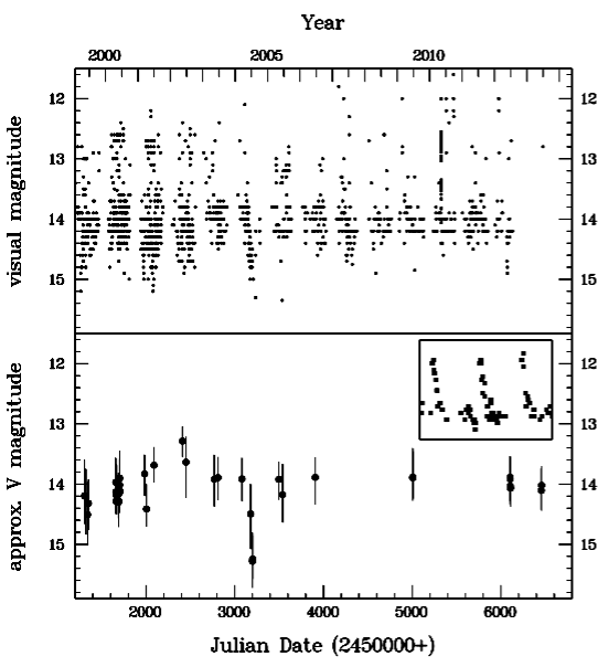
Figure 1: Top: Visual AAVSO long-term light curve of V893 Sco. Bottom: Average out-of-eclipse brightness of V893 Sco (transformed to approximate $V$-band magnitude) during each of the observing nights listed in Tab. 1. The error bars represent the total range of magnitudes observed on the respective nights (disregarding eclipses). The insert shows on an extended scale a 65-day window, centred on JD 2451700, of the AAVSO light curve with three distinct small outburst.

The AAVSO light curve also shows that the long-term behaviour of V893 Sco is different from that of most dwarf novae below the period gap. There are rather frequent low amplitude outbursts. The insert in the lower frame of Fig. 1 shows a 65-day time window around JD 2451700 which contains 3 distinct outbursts. The recurrence time during this particular section of the light curve is about 20 days. But while apart from the rather low amplitude the outburst behaviour is consistent to what is seen on other dwarf novae, the fact that during 13 years of close monitoring not a single superoutburst in this otherwise quite active system has been seen is surprising.

In order to assess the probability that superoutbursts have been missed by the AAVSO observers some simple simulations were performed. From the vast collection of superoutburst light curves of SU UMa stars published by Kato et al. (Kato09 (2009), Kato10 (2010), Kato12 (2012), Kato13 (2013)) it is seen that the plateau phase lasts at least 10 days in the overwhelming majority of cases. I conservatively assume that V893 Sco should be brighter than 12${}^{\raisebox{0.90417pt}{\scriptsize m}}_{\raisebox{1.80835pt}{\hskip 1.18999pt.}}$2 during that phase. Regarding the distribution of observing epochs in the AAVSO light curve (now also considering negative observations if the limiting magnitude is fainter than 12${}^{\raisebox{0.90417pt}{\scriptsize m}}_{\raisebox{1.80835pt}{\hskip 1.18999pt.}}$2), and if V893 Sco would have had a single superoutburst lasting 10 days starting some time during the period covered by the AAVSO observers, the simulations ($10^{6}$ trials) showed that the likelihood for the superoutburst to have been missed is $P_{\rm mis}(1)=0.26$ (in 22% of all cases due to seasonal gaps of $\approx$100 days in the light curve). This probability drops rapidly with increasing duration of the outburst. If $N$ superoutburst would have occurred, to first order the probability would be $P_{\rm mis}(N)=[P_{\rm mis}(1)]^{N}$. It would thus become very small if the recurrence time of superoutbursts would be of the order of 1 year (or less) as typically observed in SU UMa stars (unless the supercycle happens to be close to one year or multiples thereof and all the superoutbursts manage to hide in the seasonal gaps in the AAVSO light curve).

In any case, practically all dwarf novae with orbital periods below the 2-3 hour period gap are SU UMa stars, but V893 Sco, so far, cannot yet unambiguously be classified as such.

4 Eclipse profile

As already noticed in Paper I , the eclipses of V893 Sco are extremely variable. This refers equally to their depths, minimum level and shapes as can be gauged from Figs. 2 and 3 of that study. This behaviour made the authors believe the hot spot (together with part of the accretions disk) to be the eclipsed body, while the white dwarf remains uneclipsed. However, in Suzaku observations Mukai et al. (Mukai (2009)) found a partial x-ray eclipse which they attributed to a partial obscuration of the boundary layer between accretion disk and white dwarf by the secondary star. This implies that the optical eclipse should include at least a component due to the white dwarf being partially covered by the red dwarf.

The additional optical data presented here greatly increase the number of observed eclipses, enabling – in spite of the strong variability – to address the question of the eclipse shape in greater detail than was possible before. In order to overcome the difficulty caused by the strong variations of the eclipse depth the eclipses were first normalized. This is possible because in most light curves one can identify the start of eclipse ingress reasonably well even in the presence of strong flickering (see Fig. 3 of Paper I ). In all cases this was done by visual inspection. This introduces a certain degree of arbitrariness in particular when the exact phase of ingress is difficult to separate from flickering activity. However, while this increases the error margins, is does not affect the conclusions.

First, the light curves were phased according to the ephemerides derived in Sect. 5. They were then transformed from magnitudes into arbitrary intensities and normalized such that the eclipse bottom, determined as the minimum of a fitted forth order polynomial to the data points in the phase range from -0.01 to 0.01, has zero intensity, and unit intensity corresponds to the difference between the brightness at the start of ingress and eclipse bottom. All eclipses are thus brought onto the same scale. The solid line in the upper frame of Fig. 2 shows the average profile of 110 eclipses used in this exercise with a resolution of 0.001 in phase. The dotted lines delimit the uncertainty range as determined from the standard deviation of all data points within a given phase bin.

In many quiescent dwarf novae the ingress and egress phases of the eclipse profile consist of two components: Ingress starts with a steep brightness decline ascribed to the occultation of the white dwarf. It is followed by a slightly slower decline caused by the eclipse of the bright spot. When both, white dwarf and bright spot, are aligned along the line of sight from the observer to the border of the secondary star at the start of the eclipse, or if the transition is very smooth, the two components cannot be separated confidently. On the other hand, upon egress the separation is often much clearer. The white dwarf emerges from the eclipse first. Due to the different geometrical situation when looking along the opposite border of the red dwarf it takes longer for the bright spot to emerge from the eclipse. Thus, egress often occurs in two well separated steps. Classical examples of dwarf novae which exhibit this kind of eclipse profile are Z Cha (Wood et al., Wood86 (1986)), OY Car (Wood et al., Wood89 (1989)) and IP Peg (Bobinger et al., Bobinger (1999)).

The average eclipse profile of V893 Sco shows some similarity to this classical picture. The ingress cannot be separated into two distinct phases. It starts as phase $-0.019$ and may be interpreted as the simultaneous start of white dwarf and hot spot occultation. After a rounded minimum (indicating that the eclipse is not total) first a steep rise can be seen which is symmetrical to the latter part of the ingress. Apparently, this is due to the white dwarf emerging from partial eclipse. After recovering to about 2/3 of the intensity at the start of ingress, the egress levels off at phase $0.018$ (i.e. within the errors this phase and the phase of the start of ingress are symmetrical to mid-eclipse) and continues much more gradually until the eclipse ends approximately at phase $0.077$. This second part of the egress may then be taken as the hot spot egress. In contrast to what is seen in the examples quoted above there is no distinct step at the end. This may either be explained by the step being washed out in the average of many eclipses or that the hot spot has no well defined edge.

The error limits around the average eclipse profile, as shown in Fig. 2, are quite wide during the second part of the egress. This reflects a strong variability of V893 Sco after the white dwarf emerges from occultation: In many cases the egress of the hot spot is not evident in the individual light curves. To illustrate this, the lower frames of Fig. 2 show two eclipses, one with an obvious step during egress (left) and one with no trace of a hot spot eclipse (right). This can be explained by the strong ubiquitous flickering in V893 Sco which apparently outshines the hot spot easily. In the case of the cataclysmic variables Z Cha, HT Cas, V2051 Oph, IP Peg and UX UMa, Bruch (Bruch96 (1996), Bruch00 (2000)) has shown that the flickering arises mainly in the inner accretion disk, albeit with contributions from the hot spot in most of these systems. The strong variability of V893 Sco during the second part of eclipse egress, i.e. when the hot spot is still hidden behind the secondary star, shows that in this case the hot spot is not the (main) flickering light source.

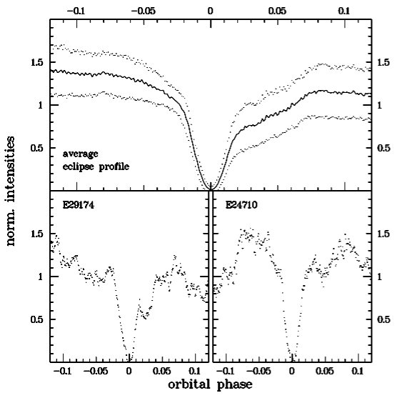
Figure 2: Top: Average normalized eclipse profile of V893 Sco (solid line) based on 110 individual eclipses. The dotted lines show the standard deviation of individual profiles with respect to the average. Bottom: Two individual eclipse profiles with (left) and without (right) a clear delay of the final egress.

This scenario can also explain the strong variability of the eclipse depth (see Fig. 2 of Paper I ). Since the eclipse of the white dwarf is only partial even at mid-eclipse about half of the inner accretion disk, where the flickering is expected to happen, remains visible. Since the short timescales of the Keplerian motion in the inner accretion disk ($\sim$$15^{\rm s}$ to complete an orbit at the surface of a typical $0.75M_{\sun}$ white dwarf; $\sim$$165^{\rm s}$ sec at a distance of 5 white dwarf radii) inhibits flickering close to the white dwarf to maintain a significant asymmetry in azimuth over the eclipse duration ($\sim$$4^{\rm m}$) the amount of eclipsed light and thus the eclipse amplitude should scale linearly with the out-of-eclipse brightness, and the factor of proportionality should be equal to the fraction of light occulted at mid eclipse.

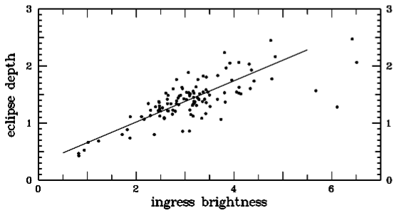
Figure 3: Eclipse depth as a function of the brightness of V893 Sco at the start of eclipse ingress, both in arbitrary intensity units. The solid line represents a linear fit to the data, disregarding the four deviating points at the right which refer to an outburst (see text).

Fig. 3 shows the dependence of the eclipse depth on the brightness at the start of eclipse ingress. Again, magnitudes have been transformed into arbitrary intensities which, however, in the present context must not be normalized. There is a clear correlation, in spite of a significant scatter which may be attributed partly to difficulties to exactly define the onset of the eclipses in the individual light curves and partly to uncertainties caused by a residual dependence of flickering on azimuth in the inner disk. The four deviating points at high ingress brightness all refer to eclipses observed on 2002, May 15/16, when V893 Sco was on the decline from an outburst (see Sec. 3). The disk structure should therefore be different during these eclipses and I disregard these points. A linear fit to the remaining data, shown as a solid line in the figure, has a slope of $0.36\pm 0.06$, suggesting that on the average about a third of the light of V893 Sco is occulted during mid-eclipse.

5 Ephemerides

Eclipse ephemerides for V893 Sco have first been derived in Paper I using a total time base of only 49 days. They have accumulated a significant error over time. Therefore this exercise is repeated here with higher precision, taking advantage of the much longer time base of 14 years.

The same method to define the eclipse timings was used here as employed in Paper I (the reader is referred to that paper for details) The eclipse epochs (including also the eclipses analysed in Paper I ) , expressed as Barycentric Julian Date in Barycentric Dynamical Time (BJD-TDB) are given in Table 2. I disregard here the data of 1999 June 21/22, because the eclipse times deviate strongly from the ephemerides derived below, suggesting that a timing error occurred during this night. Similarly, an error of the time stamps of a part of the 2013 June 10/11, observation inhibited the use of the third eclipse observed during that night.

Table 2: Eclipse Epochs.

	Eclipse	BJD-TBD		Eclipse	BJD-TBD		Eclipse	BJD-TBD
Date	Number	(2450000+)	Date	Number	(2450000+)	Date	Number	(2450000+)
1999 May 25	00000	1323.53330	2000 Jun 7	04992	1702.73250	2004 Jun 22	24433	3179.49968
	00001	1323.60957		05001	1703.41681	2004 Jun 23	24434	3179.57572
	00003	1323.76137		05002	1703.49254		24435	3179.65176
1999 Jun 11	00236	1341.46053	2000 Jun 8	05003	1703.56856		24436	3179.72767
1999 Jun 12	00237	1341.53637		05004	1703.64424	2004 Jul 13	24709	3200.46521
	00238	1341.61232		05005	1703.72061	2004 Jul 14	24710	3200.54117
	00240	1341.76433		05006	1703.79636		24711	3200.61721
2000 Apr 25	04424	1659.58695		05014	1704.40419		24722	3201.45257
2000 Apr 26	04437	1660.57400		05015	1704.48013	2004 Jul 15	24723	3201.52871
	04438	1660.65015	2000 Jun 9	05016	1704.55593	2005 May 7	28621	3497.62663
2000 Apr 27	04451	1661.63786		05017	1704.63210		28622	3497.70267
2000 Apr 28	04464	1662.62522		05018	1704.70801		28623	3497.77880
2000 May 6	04568	1670.52540		05019	1704.78413	2005 Jun 17	29172	3539.48133
	04569	1670.60127	2000 Jun 10	05029	1705.54367	2005 Jun 18	29174	3539.63342
2000 May 23	04792	1687.54082		05030	1705.61962		29175	3539.70938
	04794	1687.69242		05031	1705.69550	2006 Jun 20	34016	3907.43862
	04795	1687.76871		05032	1705.77137	2006 Jun 21	34017	3907.51460
	04796	1687.84446	2001 Mar 16	08705	1984.77784	2009 Jun 22	48471	5005.46165
2000 May 24	04805	1688.52834	2001 Apr 6	08979	2005.59115	2009 Jun 23	48472	5005.53778
	04806	1688.60412	2001 Jun 30	10097	2090.51631		48473	5005.61377
	04807	1688.68012		10098	2090.59219		48474	5005.68957
	04809	1688.83201		10099	2090.66788		48475	5005.76538
2000 May 25	04818	1689.51563	2002 May 16	14310	2410.54171		48484	5006.44943
	04819	1689.59161		14311	2410.61774	2009 Jun 24	48485	5006.52508
	04820	1689.66779		14312	2410.69363		48486	5006.60131
	04821	1689.74354		14313	2410.76953		48487	5006.67710
	04822	1689.81953	2002 Jun 24	14836	2450.49766		48488	5006.75309
2000 May 26	04831	1690.50306	2002 Jun 25	14837	2450.57328	2012 Jun 12	62757	6090.64690
	04832	1690.57923		14838	2450.64943	2012 Jun 13	62770	6091.63449
	04834	1690.73105		14839	2450.72537	2012 Jun 15	62795	6093.53328
2000 May 27	04845	1691.56675	2003 May 10	19036	2769.53553	2012 Jun 16	62808	6094.52083
	04846	1691.64260		19037	2769.61168		62811	6094.74881
	04847	1691.71863	2003 Jun 20	19588	2811.46646	2013 Jun 11	67547	6454.50234
	04848	1691.79459	2003 Jun 21	19589	2811.54245		67548	6454.57837
2000 Jun 6	04988	1702.42887		19590	2811.61860	2013 Jun 13	67586	6457.46487
2000 Jun 7	04989	1702.50459		19591	2811.69426	2013 Jun 14	67587	6457.54111
	04990	1702.58067	2004 Mar 17	23145	3081.66173		67589	6457.69266
	04991	1702.65665		23147	3081.81294		67590	6457.76880

It is not straight forward to assign error bars to the individual eclipse epochs. Requiring that the reduced $\chi^{2}_{\rm r}$ of the residuals between the observed and calculated minimum times, using the final ephemerides (see below), is equal to 1 (i.e. that the minimum times are adequately described by eq. 1) results in an error of 13.3 sec which is adopted a posteriori as the standard deviation of the data points.

A linear least-squares fit to the eclipse timings listed in Table 2 yields the $O-C$ diagram shown in the upper frame of Figure 4. It clearly shows that linear ephemerides cannot adequately describe the minimum times of V893 Sco. There is an obvious modulation of the $O-C$ values which can very well be fitted with a simple sine-curve. Therefore, a suitable description of the ephemerides takes the form

$$BJD(min)=T_{o}+P_{o}\times E+b\times E^{2}+A\,\sin\left[2\pi\left(\frac{E}{P_{1}}-\phi\right)\right]\,,$$ (1)

where $BJD$ is the Barycentric Julian Date expressed in Barycentric Dynamical Time and $E$ is the eclipse number. Here, I also include a term $b\times E^{2}$, allowing for a secular variation of the orbital period. $b$ is related to the time derivative of $P_{o}$ through ${\dot{P}_{o}}\equiv{\rm d}P_{o}/{\rm d}t=2b/P_{o}$.

Numerical values for the time $T_{o}$ of eclipse $E=0$, the mean orbital period $P_{o}$ and its derivative ${\rm d}P_{o}/{\rm d}t$, the period $P_{1}$ of the modulation of the orbit, the amplitude $A$ of the modulation and the phase $\phi$ are summarized in Table 3 (Model A) where the quantities in brackets represent the errors in the last digits. The $O-C$ diagram corresponding the these final ephemerides is shown in the lower frame of Figure 4. It is consistent with 0 and does not show any significant systematic trend over the 14 year time base. Some points close to BJD 2451700 are systematically below most of the other data. They all refer to an observing run in 2000 June. While I cannot exclude an error in the time stamps of these observations, there is also no clue for this to be the case. Therefore, there is no objective reason to exclude these data from the analysis.

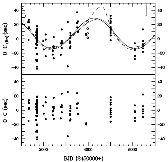
Figure 4: Top: Observed minus calculated eclipse epochs for V893 Sco, using the best fit linear ephemerides. The filled and open symbols represent eclipses of this paper and of Mukai et al. (2009), respectively. The solid line is the best fit sine curve to the filled symbols. The dotted and dashed curves represent solutions for an eccentric orbit of an assumed third body with eccentricity $e=0.3$ and $e=0.6$, respectively (see Sect. 6.2). An empirical estimate for the error bars of the individual points is shown in the upper right corner. Bottom: Observed minus calculated eclipse epochs using the final ephemerides described by Eq. 1.

Table 3: Ephemerides for V893 Sco.

		Model A	Model B
$T_{o}$	(BJD)	2451323.533413 (15)	2451323.533433 (15)
$P_{o}$	(days)	0.07596146514 (52)	0.07596146589 (53)
…	(hours)	1.823075163 (13)	1.823075181 (13)
${\rm d}P_{o}/{\rm d}t$		$6(3)\,10^{-13}$	–
$P_{1}$	(cycles)	48992 (1102)	48989 (1259)
…	(days)	3721 (84)	3721 (95)
$A$	(days)	0.000258 (27)	0.000258 (26)
…	(sec)	22.3 (2.3)	22.3 (2.3)
$\phi$		0.537 (11)	0.537 (50)

While the period is well determined this is not so for the period derivative. Nominally, V893 Sco exhibits a slight secular increase in the orbital period. While there may be mechanisms which lead to a period increase over the scale of the observational time base this is contrary to the expected secular period evolution of cataclysmic variables unless V893 Sco is a period bouncer. This, however, is rather unlikely since it does not exhibit any behaviour considered characteristic for CVs which have evolved beyond the period minimum (Zharikov et al., Zharikov (2013)) such as broad Balmer line absorption troughs (see spectra shown by Mason et al. Mason (2001)) or persistent orbital double humps in the light curve. Moreover, V893 Sco exhibits rather frequent (normal) dwarf nova outbursts, in contrast to the rare (WZ Sge type) superoutbursts expected for period bouncers. Therefore, considering the small numerical value of ${\rm d}P_{o}/{\rm d}t$ and the large relative error, $\dot{P_{o}}$ can at most be considered marginally significant and I will neglect it in the following.

Meeting a concern raised by the referee that the parameters $A$ and $b$ in eq. 1 are likely to be highly coupled I also calculated a solution with $b$ fixed to zero (Model B in Tab. 3). All other parameters change only insignificantly (much less than their errors) with respect to the values for Model A which were used for the subsequent calculations. But Model B would lead to identical results within the numerical accuracy of all quantities quoted below.

When recalculating the ephemerides I did not consider the eclipse timings measured by Mukai et al. (Mukai (2009)) because they determined eclipse ingress and egress times in a way such that the eclipse centre (calculated as the mean between ingress and egress) might be systematically offset from the eclipse centre as determined here. However, as a consistency check the results of their timings, after transforming the heliocentric Julian Dates quoted by them into barycentric Julian Dates, are included in the $O-C$ diagram of Fig. 4 (upper frame) as open symbols. It is seen that they fit in quite satisfactorily.

6 The cyclic period variations

Cyclic period variations derived from eclipse timings are not unusual in cataclysmic variables. On the contrary, they appear rather to be the rule. Borges et al. (Borges (2008)) compiled a list of 14 systems exhibiting this phenomenon which contains most of the brighter eclipsing CVs, well observed over a long time base. An updated version was published by Pilarčík et al. (Pilarcik (2012)), who also included some post-common envelope binaries (PCEBs) with similar period variations. HU Aqr (Qian et al. Qian11 (2011), Goździewskiet al. Gozdziewski (2012)) and RR Cae (Qian et al. Qian12 (2012)) may be added to this list.

Discarding apsidal motions as the origin of the period variations on the grounds that the orbital eccentricity of these strongly interacting binaries must be essentially zero, it was for a long time believed that they could be explained by magnetic cycles in the secondary stars of these systems via the so-called Applegate mechanism (Applegate Applegate92 (1992)). However, unless a significantly more energy efficient mechanism can be identified (see Lanza et al. Lanza (1998)) this explanation has been shown not to work in many individual cases (e.g. AC Cnc: Qian et al. Qian07 (2007); Z Cha: Dai et al. Dai09b (2009); TV Col: Dai et al. Dai10b (2010); UZ For: Potter et al. Potter (2011); DQ Her: Dai & Qian Dai09a (2009); NN Ser: Brinkworth et al. Brinkworth (2006); QS Vir: Parsons et al. Parsons (2010)) mainly because the energy required to drive the observed period change is more than the total energy output of the star.

Therefore, researchers started to focus on light travel time effects to explain the period variations. In this scenario the binary rotates around the centre of gravity with a third object. Depending on its distance from the centre of mass eclipses will be observed slightly early or late and thus the orbital period will appear to be variable with the period of this extra motion of the binary. Under this hypotheses the observed cyclic period changes can in many cases be explained by the presence of a giant planet or a brown dwarf orbiting around the binary (T Aur: Dai & Qian Dai10a (2010); RR Cae: Qian et al. Qian12 (2012); DQ Her: Dai & Qian Dai09a (2009); DP Leo: Qian et al. 2010a , Beuermann et al. Beuermann11 (2011); QS Vir: Qian et al. 2010b ; HS0705+6700: Beuermann et al. 2012a ).

Adopting this basic hypotheses the interpretation of the observations is relatively straightforward in the quoted cases. However there are other examples where the period variations are more complex and two planets (and, additionally, often a secular period decrease) are required to explain them within the light travel time scenario. The question of long-term stability of such planetary systems then arises, and it may not be easy (or even impossible) to find a configuration which is compatible with observations and at the same time ensures the survival of the planetary system on secular timescales. Examples are HU Aqr (Qian et al. Qian11 (2011), Horner et al. Horner11 (2011), Goździewski et al. Gozdziewski (2012) Wittenmyer et al. Wittenmyer (2012)), NN Ser (Qian et al. Qian09 (2009), Brinkworth et al. Brinkworth (2006), Beuermann et al. Beuermann10 (2010), Hessman et al. Hessman (2011), Marsh et al. Marsh (2014)) and HW Vir (Lee et al. Lee (2009), Beuermann et al. 2012b , Horner et al. Horner12 (2012)).

Another important requirement for the light travel time interpretation to be viable arises from evolutionary considerations. The orbit(s) must be such that the planet(s) not only can survive the common-envelope phase, but they must also have been stable in the previous phase when the stellar components had a much larger separation. A related question is the fraction of PCEBs which show evidence for the presence of planets as compared to the fraction of their progenitors with planetary systems. Zorotovic and Schreiber (Zorotovic (2013)) find that 90% of detached PCEBs with accurate eclipse time measurements show period variations that might indicate the presence of a third body. However, their main sequence progenitors are quite unlikely to be hosts of giant planets ($\leq 10\%$). These authors therefore conclude it to be more likely that the period variations in PCEBs are caused by second generation planets, formed from remnants of the common envelope which were not expelled from the binary system, or that they are due to some other cause altogether which so far has not yet been identified.

Finally, the question of the uniqueness of a given solution must be addressed. More than once a published solution was shown to be untenable or required a significant revision when more eclipse timings were added to the available data (e.g. DP Leo: Qian et al. 2010a vs. Beuermann et al. Beuermann11 (2011); NN Ser: Qian et al. Qian09 (2009) vs. Parsons et al. Parsons (2010) and Beuermann et al. Beuermann10 (2010); HW Vir: Lee et al. Lee (2009) vs. Beuermann et al. 2012b ). Independent analysis of the same data set, using different criteria, may also lead to discrepant results (e.g. HU Aqr: Qian et al. Qian11 (2011) vs. Goździewski et al. Gozdziewski (2012); HW Vir: Lee et al. Lee (2009) vs. Horner et al. Horner12 (2012)). Understandably this problem is more severe for systems with complex period variations which cannot be explained by the effect of a single planet.

In contrast to many of the cases quoted above the period variations of V893 Sco are comparatively simple and can well be approximated by a single sine curve. In spite of the mentioned caveats it is therefore close at hand to interpret them as a light travel time effect caused by a third body in the system; and I will do so in the following. However, first I will verify if the Applegate mechanism can safely be rejected.

6.1 The Applegate mechanism

As mentioned above it has been shown that the Applegate mechanism cannot explain the period variations observed in several CVs and pre-CVs because the secondary star does not generate enough energy to drive it. Here, I will briefly verify if this is also the case for V893 Sco.

In order to explain the full amplitude $2A$ of the observed $O-C$ variations over a time span of $P_{1}/2$ an average period derivative of $\delta P/P_{0}=1.44\times 10^{-7}$ is required. This implies in a total period change of $\Delta P=3.5\times 10^{-3}\,{\rm s}$.

For an approximate calculation of the total energy generated by the secondary star I assume that its radius $R_{2}$ and effective temperature $T_{2}$ are equal to the values derived from the semi-empirical CV donor star sequence of Knigge et al. (Knigge11 (2011)) at the orbital period of V893 Sco. This gives $R_{2}=0.174\,R_{\sun}$ and $T_{2}=3087$ K. The luminosity is then $L_{2}=4\pi R_{2}^{2}\sigma T_{2}^{4}=2.47\times 10^{-3}\,L_{\sun}$ where $\sigma$ is the Stefan-Boltzmann constant. Over the time required to change the orbital period by $\Delta P$ (i.e. half the period of the cyclic variation of the eclipse timings) this adds up to $1.5\times 10^{39}\,{\rm erg}$.

On the other hand, using eqs. 27 and 28 of Applegate (Applegate92 (1992)) the energy required to redistribute the angular momentum between the core and the shell of the star can be calculated. Being interested in the minimum of the necessary energy I neglect the angular velocity of differential rotation in Applegate’s eq. 28: $\Omega_{\rm dr}=\Omega_{\rm shell}-\Omega_{\rm core}=0$. Assuming component masses of $M_{2}=0.134\,M_{\sun}$ and $M_{1}=0.75\,M_{\sun}$ (see Sect. 6.2) for V893 Sco, the component separation follows from the orbital period and Kepler’s third law. Furthermore, a simple polytrope model with index $n=1.5$, appropriate for fully convective stars, is used to calculate the interior mass distribution and the moments of inertia of the core and the shell as a function of the assumed shell mass. The minimum energy is then found to be $1.8\times 10^{39}{\rm erg}$ at a shell mass of $0.035\,M_{\sun}$. Although not by a large factor, this is still more than the total energy generated by the star.

Since it cannot be assumed that the entire energy production is used to power the angular momentum distribution between layers of the star, Applegate’s mechanism can thus be excluded as an explanation for the cyclic period change observed in V893 Sco, unless an alternative energy source can be identified.

Following a suggestion of Raymundo Baptista (private communication) I make the ad hoc assumption that orbital energy of the secondary can be tapped to drive the Applegate mechanism (without trying to specify a physical mechanism for this to happen). Lowering the secondary star in the gravitational potential of the primary will release potential energy. Assuming Keplerian orbits, a part of this will be used up for the faster motion of the secondary on the lower orbit, but the rest will be available for other purposes. I therefore calculated the change $\Delta P$ in the orbital period required for this rest to be equal to the minimum energy necessary to drive the Applegate mechanism. Adopting the parameters of V893 Sco, $\Delta P=-8.2\,10^{-5}$ sec. Assuming that this energy must become available over the time it takes to complete half of a cycle of the period variations this translates into a time derivative of ${\rm d}P_{o}/{\rm d}t=-5.1\,10^{-13}$. This is of the order of the error of the formal time derivative quoted in Tab. 3. The cumulative effect on the $O-C$ diagram over the whole time base of the observations would be $\approx$1 sec, undetectable in view of the scatter of the data points in Fig. 4.

The picture drawn here is, of course, greatly simplified .It assumes that the entire available orbital energy is used to power the Applegate mechanism. If only a part of it goes into this channel $\Delta P$, as derived above, is a lower limit. On the other hand, apart from orbital energy other energy sources may be accessible. Finally, the necessary energy for the Applegate mechanism adopted here is the minimum value: If the shell mass is different from $0.035\,M_{\sun}$ or if $\Omega_{\rm dr}>0$ more energy is required. There are thus at least three unknown parameters which complicate the picture, not to speak of the total ignorance of a physical mechanism to explain how orbital energy can be tapped.

Therefore, in conclusion it can be stated that under favourable circumstances a secular period decrease smaller than can be detected with the available data is, in principle, able to provide the energy necessary to drive the Applegate mechanism. But, for the time being, this possibility is only speculative.

6.2 Basic parameters of the third body

Therefore, I will now interpret the cyclic variations in the $O-C$ diagram as being caused by the motion of a third body. Subsequently the indices ${\cal A}$ and ${\cal B}$ will be used for the white dwarf and the mass transferring red dwarf in V893 Sco, and ${\cal P}$ for the third body. The index “${\rm inn}$” refers to the inner binary, composed of components ${\cal A}$ and ${\cal B}$, while “${\rm out}$” refers to the outer orbit of ${\cal P}$ around ${\cal AB}$.

The shape of the $O-C$ curve does not suggest significant deviations from a pure sinusoidal signal, and the scatter of the data points does not warrant a fit of a more complicated function such as that needed to describe an eccentric orbit. Therefore, the motion of the third body around the inner V893 Sco binary is assumed to be circular. Let $c$ be the speed of light and $i_{\rm out}$ the inclination of the outer orbit to the line of sight. Then the amplitude $A$ of the eclipse timings modulation translates into a projected distance of component ${\cal AB}$ to the centre of gravity of $a_{\cal AB}\sin i_{\rm out}=A\times c=(6.7\pm 0.7)\times 10^{9}\,{\rm m}$. With the total mass of the inner binary system, $M_{\cal AB}$, the mass of the third body, $M_{\cal P}$, the modulation period $P_{1}$, and the gravitational constant $G$, the mass function can be written as

$$f(m)\equiv\frac{\left(M_{\cal P}\sin i_{\rm out}\right)^{3}}{\left(M_{\cal AB}+M_{\cal P}\right)^{2}} = \frac{4\pi^{2}}{G}\frac{\left(a_{\cal AB}\sin i_{\rm out}\right)^{3}}{P_{1}^{2}}$$ (2)

$$= \left(1.7\pm 0.5\right)\,10^{24}\,{\rm kg}\,.$$

In order to get a handle on the mass of the third body from this equation, information about the inclination of the outer orbit and the mass of the inner binary is required. For both quantities no direct measurements exist.

Based on the empirical relation between the mass of the donor stars in cataclysmic variables and the binary period (Warner, Warner95 (1995)), Matsumoto et al. (2000) estimate a mass of $M_{\cal B}=0.15\,M_{\sun}$ for V893 Sco. Together with the constrain on the orbital inclination $i_{\rm inn}\ga 70\degr$ imposed by the presence of eclipses in the light curve and the amplitude of the radial velocity curve of the $H\alpha$ emission line (assuming it to reflect the motion of the white dwarf) they estimate $M_{\cal A}\approx 0.5-0.6\,M_{\sun}$. Mason et al. (Mason (2001)) used the secondary star mass – period and mass – radius relations of Howell & Skidmore (Howell (2001)) to derive $M_{\cal B}=0.175\,M_{\sun}$ and $R_{\cal B}=0.196\,R_{\sun}$. They then iteratively used relations involving $M_{\cal A}$, $M_{\cal B}$, $R_{\cal A}$, $R_{\cal B}$, $i_{\rm inn}$, the accretion disk radius, and the bright spot radius and azimuth to get $M_{\cal A}=0.89\,M_{\sun}$. The secondary star mass of $M_{\cal B}=0.15\,M_{\sun}$ adopted by Mukai et al. (Mukai (2009)) is based on Patterson’s (Patterson (1984)) empirical mass-period relationship. They then assumed a mass ratio for the inner binary of $q_{\cal A,B}=0.25$ to obtain a white dwarf mass of $M_{\cal A}=0.58\,M_{\sun}$. A slightly lower value of $M_{\cal B}=0.134\,M_{\sun}$ for the secondary star mass follows from the semi-empirical CV donor star sequence of Knigge et al. (Knigge11 (2011)). Knigge (Knigge06 (2006)) considers $M_{\cal A}=0.75\,M_{\sun}$ as the mass of a white dwarf in a typical cataclysmic variable.

While the differences in the various $M_{\cal B}$-values are small and not critical in the present context, all quoted values of the primary star mass are based on uncertain assumptions. Here, I will adopt the mass $M_{\cal A}=0.75\,M_{\sun}$ of Knigge (Knigge06 (2006)), assigning a generous error bar of $0.25\,M_{\sun}$ to $M_{\cal A}$ which encompasses the range of masses quoted in the literature. Since in the following calculation only the sum $M_{\cal AB}=M_{\cal A}+M_{\cal B}$ enters this error is assumed also to account for the much smaller error of the secondary star mass. Thus, $M_{\cal AB}=(0.88\pm 0.25)\,M_{\sun}$.

A relation between the inclination of the outer orbit and the mass of the third body can then be constructed which is shown in Fig 5 where the mass is expressed in units of Jupiter masses. The dashed lines indicate the $1\sigma$ error limits.

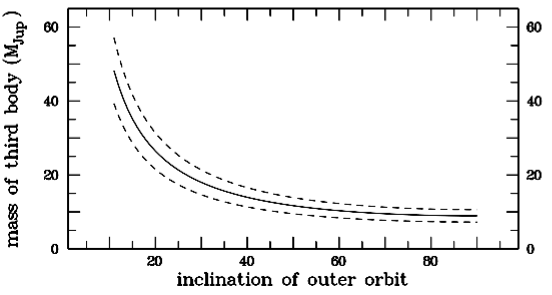
Figure 5: Mass of the third body as a function of the inclination of the outer orbit to the line of sight. The dashed curves indicate the $1\sigma$ error limits.

Knowing the orbital period of the third body and the component masses Kepler’s third law yields immediately its distance to the central binary: $a_{\rm out}={4.5\pm 0.4}\,{\rm AU}$. Due to the dependence of the mass of the third body on $i_{\rm out}$ there is a very slight increase with the inclination of the orbit. This is, however, wholly negligible within the errors which are strongly dominated by the uncertainty of the white dwarf mass.

If the original binary star which developed into a CV and the third body were formed via fragmentation of the same rotating interstellar cloud, or if the third body coalesced from a circum-binary disk (and if the orbital inclination did not suffer from a significant perturbation during the subsequent evolution) the angular momentum of the inner and outer orbits should be approximately aligned. Thus, $i_{\rm out}\approx i_{\rm inn}$. The presence of eclipses prove V893 Sco to have a high inclination. Mason et al. (Mason (2001)) estimate it to be $72\aas@@fstack{\circ}5$, while Mukai et al. (Mukai (2009)) derive a slightly higher value of $74\aas@@fstack{\circ}2$. Fig. 5 shows that in this region the relation between the mass of the third body and the inclination of the outer orbit is almost flat and $M_{\cal P}\approx 9.5\,M_{\rm Jup}$. Therefore, if the inner and outer orbits are in fact aligned, the third body has a mass which would classify it as a giant planet. I will therefore subsequently not distinguish between the terms “third body” and “planet”.

In the previous discussion the assumption of a circular orbit of the third body was justified with the scatter of the data points in the $O-C$ diagram. While the data thus do not suggest a finite orbital excentricity $e$, they also do not exclude values of $e>0$. Respective solutions were investigated, using the prescriptions of Irwin (Irwin (1952)). A formal fit of an eccentric orbit to the $O-C$ values shown in the upper frame of Fig. 4 was not conclusive because due to the scatter the data permit an infinity of formal solutions the goodness of which are statistically indistinguishably. For this reason fits were calculated, using the Simplex algorithm (Caceci & Cacheris Caceci (1984)), keeping the eccentricity fixed and permitting the other orbital parameters to be adjusted. As illustrative cases, the dotted and dashed curves in Fig. 4 show solutions for $e=0.3$ and $e=0.6$, respectively. They fit the data just as well as the sine curve does. Reminding the reader that the observational timing error of the eclipse epochs was determined such that $\chi^{2}_{\rm r}$ is unity in the case of a purely sinusoidal shape of the cyclic period variations (Sect. 5), $\chi^{2}_{\rm r}=0.99\,(1.01)$ for $e=0.3\,(0.6)$ is found. It is thus not possible to prefer one solution over the other on statistical grounds. Therefore, the orbital eccentricity of the third body is not constrained by the current data.

6.3 Evolutionary considerations

Let us now address the question whether the existence of a planet with the characteristics derived in the previous section is compatible with the evolution of the V893 Sco system from a wide binary to a cataclysmic variable. This implies that the planet would have existed before the common envelope (CE) phase. The subsequent considerations are not meant to substitute a rigorous in-depth study. The aim is just to get a general idea if serious problems become obvious or not.

As criterion for the planetary scenario to be viable from the evolutionary point of view it is assumed that the orbit of the planet is larger than the radius $R_{\rm CE}$ of the common envelope. $R_{\rm CE}$ is approximated by the radius $R_{\rm max}$ which a single star has when its core mass is equal to the mass of the white dwarf in V893 Sco. For 0.75 (0.5, 1.0) $M_{\sun}$, i.e. the nominal white dwarf mass adopted in the previous section, minus and plus the assumed uncertainty, the core mass – radius relation for giants as given by Joss et al. (Joss (1997)) yields $R_{\rm max}=2.8$  (0.9, 4.6) AU.

This radius cannot directly be compared to that of the orbit of the third body as derived in the previous section because the distance between the planet and the inner binary will have changed during the evolution of the system. In a first approximation only the mass loss of the primary star during the common envelope phase is regarded which leads to a widening of the planetary orbit. Therefore, the radius of the progenitor star must be compared to the original separation of the third body from the inner binary. To this end one needs to know the mass of the white dwarf progenitor. Several initial – final mass relations for white dwarfs have been published in the literature. For the nominal white dwarf mass of $M_{\cal A}=0.75\,M_{\sun}$ the relation of Zhao et al. (2012) yields a mass of $M_{\rm prog}=(4.1\pm 1.2)\,M_{\sun}$ for the progenitor star. This is equal to the upper limit of progenitor star masses for which their relation is valid. The lower limit of the validity range ($1.1M_{\sun}$) corresponds to a white dwarf mass of $(0.53\pm 0.05)\,M_{\sun}$, close to the lower limit adopted in the previous section. Similarly, eq. (1) of Salaris et al. (Salaris (2009)) gives $M_{\rm prog}=3.4\,M_{\sun}$, while their alternative eq. (2) leads to $M_{\rm prog}=3.1\,M_{\sun}$. For the lower white dwarf mass limit the relations of Salaris et al. (Salaris (2009)) have no solutions while for the upper limit in both cases $M_{\rm prog}=6.4\,M_{\sun}$. Finally, using eqs. (2) and (3) of Catalán et al. (Catalan (2008)) I find $M_{\rm prog}=3.2\pm 0.2\,M_{\sun}$ ($0.7\pm 0.2\,M_{\sun}$; $5.0\pm 0.3\,M_{\sun}$) for $M_{\cal A}=0.75\,M_{\sun}$ ($0.5\,M_{\sun}$; $1.0\,M_{\sun}$). To be specific and since I am only interested in an order of magnitude estimate, I adopt $M_{\rm prog}=3.5\,M_{\sun}$ with lower and upper limits of 1.0 and 5.5 $M_{\sun}$, respectively.

In order to calculate the radius $a_{\rm preCE}$ of the orbit of the third body before the CE phase it is assumed that its orbital angular momentum $m$ is the same before and after that phase (i.e, it remains outside the common envelope). Knowing the mass of the planet and its current orbital radius and period the angular momentum can be calculated which can then be used to derive the original period $P_{\rm preCE}$ as a function of $a_{\rm preCE}$. Kepler’s third law together with the component masses before the common envelope phase provided a second relation between $P_{\rm preCE}$ and $a_{\rm preCE}$. This enables to pin down the radius. It turns out that $a_{\rm preCE}\propto(m/M_{\cal P})^{2}$. Since $m$ is also proportional to $M_{\cal P}$ the dependence on the planetary mass cancels out and $a_{\rm preCE}$ does not depend on the mass and thus (via eq. 2) on the inclination of the outer orbit.

Assuming the mass of the secondary star not to change during the common envelope phase, $a_{\rm preCE}=1.1\pm 0.6\,{\rm AU}$ in the case of the nominal white dwarf mass ($0.75\,M_{\sun}$) and $a_{\rm preCE}=3.7\pm 2.0$ ($0.7\pm 0.4$) AU in the case of the lower (upper) limit, respectively. Here the errors do not include the (possibly major) contribution due to the error of $M_{\rm prog}$.

Table 4: Relationship between the white dwarf mass $M_{\rm WD}$ of V893 Sco, the mass $M_{\rm prog}$ of its progenitor, the maximum radius $R_{\rm max}$ of the progenitor and the radius $a_{\rm preCE}$ of the planet before the CE phase

$M_{\rm WD}\,(M_{\sun})$	0.5	0.75	1.0
$M_{\rm prog}\,(M_{\sun})$	1.1	3.5	5.5
$R_{\rm max}$ ($\approx R_{\rm CE}$)  (AU)	0.9	2.8	4.6
$a_{\rm preCE}\,({\rm AU})$	3.7	1.1	0.7

Summarizing, in Table 4 the mass of the white dwarf progenitor, the maximum radius that it would have as a single star (which is expected to be of the order of the radius of the CE) and the initial radius of the planetary orbit for the three adopted values of the white dwarf mass are listed, the current orbital radius of 4.5 AU of the planet having been used in the calculations. Comparing $a_{\rm preCE}$ with $R_{\rm max}$ shows that in the framework of the simple scenario explored here the third body orbit should have been larger than the radius of the white dwarf progenitor at the onset of the common envelope phase only if the primary of V893 Sco has a mass somewhat less than the average for CVs (but still within the range of primary masses found in cataclysmic variables). Thus, the presence or not of a conflict depends decisively on the white dwarf mass. A possible problem could be alleviated if the assumption of angular momentum conservation is not valid. The planet could have lost angular momentum due to friction if it revolved within the outer reaches of the CE or a dense wind from the inner binary. Depending on the balance of angular momentum loss and decrease in the total system mass this could have caused an smaller increase in the orbital radius than in a scenario without loss of angular momentum, or even a decrease.

A more rigorous investigation of the fate of planets considering the evolution of the parent star through the giant phase has recently been performed by Nordhaus & Spiegel (Nordhaus (2013)). Their scenario differs somewhat from the current one because they only regard planets around single stars, not binaries. However, since in the above simplified calculations the binary nature of the V893 Sco progenitor system did not enter explicitly a comparison should still be possible. In fact, the detailed study of Nordhaus & Spiegel (Nordhaus (2013)) does confirm the results obtained here. Their Fig. 3 shows that for a stellar mass equal to the minimum mass considered presently, a 10 $M_{\rm Jup}$ mass planet with an orbital radius $>$2.5 AU should escape engulfment by the parent star. For a $\sim$$1.5\,M_{\sun}$ star (equivalent to a white dwarf of $0.57\,M_{\sun}$ according to Catalán et al., Catalan (2008)) this limit is $\sim$3.5 AU.

Another question regards the stability of the planetary orbit before the common envelope phase in a situation where its radius is not necessarily large compared to the separation of the binary star components. This issue was investigated by Holman & Wiegert (Holman (1999)) for planets on circular orbits and coplanar with the binary orbit. In the most favourable situation of a binary with negligible orbital eccentricity and assuming a reduced mass ratio $\mu=M_{\cal B}/(M_{\rm prog}+M_{\cal B})=0.11$ (corresponding to the lower limit of the masses for V893 Sco) the planetary motion should be stable if the ratio between the semi-major axis of the planetary orbit is more then twice that of the binary orbit. As Tab. 4 shows this is indeed the case if the mass of the white dwarf in V893 Sco is on the low side.

I therefore conclude that these evolutionary considerations do not reveal insurmountable obstacles to the presently regarded interpretation of the observed cyclic period changes of V893 Sco if the white dwarf is not significantly more massive than $\approx 0.5-0.6\,M_{\sun}$ as estimated by Matsumoto et al.  (2000).

7 Frequency analysis

Warner (Warner04 (2004)) gives an overview over the rich phenomenology of oscillations in the brightness of many cataclysmic variables. These are generally divided into two classes termed dwarf nova oscillations (DNOs) and quasi-periodic oscillations (QPOs).

DNOs are normally (but not exclusively) observed in dwarf novae during outburst. They are of low (some millimagnitudes) and often strongly variable amplitude and usually have periods in the general range of a couple of seconds up to about a minute. They exhibit a wide range of coherence: Over the course of hours the periods can change by many seconds, but they also may remain stable on the millisecond level. Warner et al. (Warner03 (2003)) also introduce a second kind of DNOs which they term “longer period DNOs (lpDNOs)” with periods typically 4 times longer than normal DNOs.

Quasi-periodic oscillations have longer periods than DNOs; of the order of several hundred seconds. They are more elusive than DNOs because they are much less coherent. In general, they vanish after only a handful of periods [see Warner (Warner04 (2004)) for a description of their phenomenology and their relationship to DNOs]. This makes it difficult to distinguish them from the ubiquitous stochastic flickering activity in CVs. Therefore Warner suspects that “some reclassification [between flickering and QSOs] may be necessary; some of the flickering and flaring commented on in the CV literature has a QPO look about it”. On the other hand, the opposite may also be true. An accidental superposition of unrelated flickering events occurring on similar time and magnitude scales may well mimic QPOs. I will investigate the probability for this to happen in Sec. 7.1.1. Moreover, if individual flares in the flickering activity of CVs are not independent but physically connected, they may well assume the characteristics of QSOs. The borderline between flickering and QSOs then becomes blurred and the question may be raised if there is a conceptual difference between these two phenomena at all.

Bruch et al. (Paper I ) were the first to claim the detection of QPOs with a period of 342 sec in V893 Sco in the light curve of 1999 June 21/22. Warner et al. (Warner03 (2003)) find that the star “frequently has large amplitude QSOs”, but they give details of only one observation on 2000 June 1, when V893 Sco exhibited QSOs with a period of 375 sec concurrently with DNOs at 25.2 sec which appeared only during part of the observing run. Pretorius et al. (Pretorius (2006)) did not observe QSOs but report DNOs with a period of 41.76 sec during a 0.9 hour section of a light curve obtained on 2003 May 21.

In order to search for oscillations in the light curves of V893 Sco presented in this paper a frequency analysis at high, medium and low frequencies was performed. Here, low frequencies are understood to refer to variations on timescales $\tau\geq 15^{\raisebox{0.90417pt}{\scriptsize m}}$. This includes the orbital period and thus the range typical for positive or negative superhumps observed in many CVs. Positive superhumps are restricted to systems with superoutbursts – which are not observed in V893 Sco – and some novalike systems (permanent superhumpers). They are therefore not expected in the present case. On the other hand, negative superhumps are sometimes observed in different types of CVs (Wood & Burke, Wood07 (2007)), including dwarf novae. Medium frequencies are defined to encompass the range $15^{\raisebox{0.90417pt}{\scriptsize m}}\geq\tau\geq 2^{\raisebox{0.90417pt}{\scriptsize m}}$, where QPOs are expected to be observed if they are present, and high frequencies refer to $\tau\leq 2^{\raisebox{0.90417pt}{\scriptsize m}}$, the typical range for DNOs. In all cases the eclipses were masked before performing the analysis.

In view of the strong flickering variability which easily masks low amplitude oscillations the light curves were pre-whitened in the following way: For the high frequency analysis the light curves were binned in intervals of $2^{\raisebox{0.90417pt}{\scriptsize m}}$. A spline was then fitted to the resulting data points and subsequently subtracted from the original data. This procedure removes – if not completely – to a large degree variations on timescales above those defined by the data binning. For the medium frequency analysis the data were prepared in a similar manner, binning the light curves in intervals of $15^{\raisebox{0.90417pt}{\scriptsize m}}$. No pre-whitening was performed for the low frequency analysis. Power spectra of light curves were then calculated using the Lomb-Scargle algorithm (Lomb Lomb (1976), Scargle Scargle (1982), Horne & Baliunas Horne (1986)).

7.1 Medium frequencies and the interpretation of peaks in power spectra

I will start the discussion concentrating on medium frequencies because this is the range where the most interesting results are observed and where previous studies reported the detection of oscillations (Paper I , Warner et al. Warner03 (2003)). Apparently significant signals were also found in the power spectra of other light curves of the present study. However, before accepting them blindly as real it is appropriate to raise the question of whether a peak in a power spectrum may be regarded as caused by an oscillation in the stellar light due to a real physical phenomenon or whether it is merely due to an accidental superposition of independent random events.

As already hinted at above, it is not trivial to assess the significance of a peak in a power spectra of light curves of cataclysmic variables. The presence of strong flickering easily causes signals to be present at apparently stochastically distributed frequencies, reflecting merely the typical timescales on which strong flickering flares occur. It is therefore not obvious how to distinguish between QSOs and pure flickering (if these are really distinct phenomena).

In order to get a feeling for the probability that flickering could cause power spectrum signals that mimic apparently significant oscillations some numerical experiments are first performed. It will then be tried to estimate the probability that the highest peak in the power spectrum of each of the available light curves is significant or not.

7.1.1 Numerical experiments

For the numerical experiments three related, but slightly different procedures are pursued which will be referred to as models 1 – 3 subsequently. They consist of the frequency analysis of light curves, the individual points of which have been stochastically shuffled.

To generate the models the data points of a real light curve (after subtraction of variations on the timescale above 15 minutes as described above) were reshuffled in order to result in a new light curve which maintains the original data points, but in a random order. Repeating this procedure many times and comparing the power spectra of the randomized light curves with that of the original data should give an indication of the distribution of peaks caused by purely random flickering.

However, in reshuffling the original data points one has to consider that they are not independent but correlated on the flickering timescale. Using the light curve of 2000 June 7/8, as reference this timescale was found to be 75 seconds, as determined from the e-folding time of the autocorrelation function of the original light curve. Therefore sections of 75 seconds (15 data points) of the light curve were shuffled, creating 10 000 randomized versions of the same lengths. The corresponding power spectra were then calculated.

The difference between models 1, 2 and 3 is as follows: In creating model 1, the original light curve was cut into small segments of 75 seconds duration each. The shuffled light curves consist of randomly concatenated segments until the resulting data set has the same number of points as the original one, permitting to pick the same section more than once. Thus, an individual shuffled light curve may contain repeated sections, while other parts of the original curve are not used. Model 2 is the same as model 1, however, without permitting to pick the same section repeatedly. Therefore, all data points of the original light curve are used once and only once. For model 3, 75 second sections of the original light curve with arbitrary starting points were concatenated until the resulting curve has the same length as the original one.

The different models yielded results which were consistent with each other. Therefore, I only discuss the outcome of model 2, which is summarized in Tab. 5 and Fig. 6. The figure shows in panel (a) the power spectrum of the original data. It has a couple of peaks in the frequency range below 3 mHz, but none of these is outstanding and would thus suggest a periodic or quasi-periodic oscillation, with the exception of the peak close to 2.85 mHz. Most of the power spectra of the shuffled data are inconspicuous. However, in 2.2% of all cases the highest power spectrum peak of a randomize light curve was higher than the highest peak corresponding to the original data [$N({\rm max>max_{real}})$ in Tab. 5], in the most extreme case by 38% [$\Delta({\rm max})$]. This is shown in panel (b) of Fig. 6. Indeed, on the basis of that power spectrum an uncritical observer might claim the presence of several discrete periodicities in the stellar light!

Table 5: Frequency analysis of shuffled light curves.

reference light curve	BJD 2451702
$N({\rm max>max_{real}})$ (%)	2.2
$\Delta({\rm max})$ (%)	38
$N({\rm contrast>2.5})$ (%)	0.04
$N({\rm contrast>2.0})$ (%)	0.7
$N({\rm contrast>1.5})$ (%)	6.7

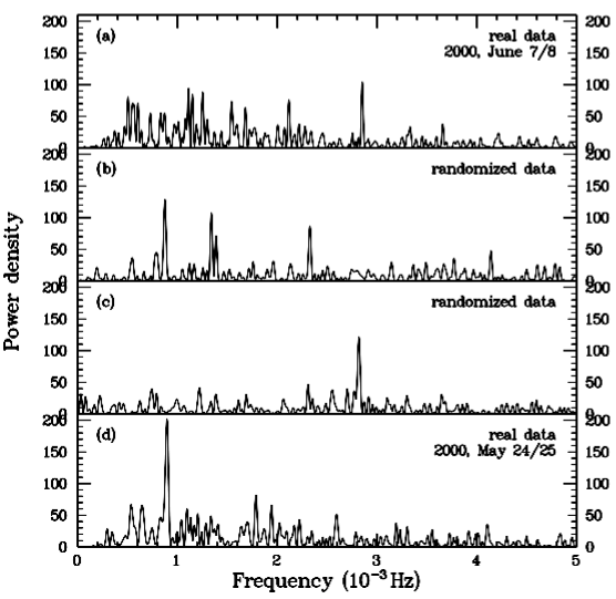
Figure 6: Panel (a): Power spectrum of the original light curve of 2000 June 7/9, after removal of the eclipses and variations on timescales longer than $\approx$$15^{\rm m}$. Panel (b): Power spectrum of the randomized light curve with the highest peak in 10 000 trials. Panel (c): Power spectrum of the randomized light curve with the largest contrast between the highest and the second highest peak. Panel (d): Power spectrum of the original light curve of 2000 May 24/25. See text for details.

Since the human eye is easily deceived by a high contrast between the dominating power spectrum peak and the secondary peaks, suggesting an outstanding peak to be due to a real signal, the ratio between the highest and the second highest peak in the power spectra of the randomized data sets was also investigated. In 0.02% (0.83%, 8.67%) of all cases the dominant peak reached more than 2.5 (2.0, 1.5) times the power of the second strongest peak. These numbers are also listed in Tab. 5. The power spectrum of a randomized data set with the highest contrast between the primary and secondary peaks is shown in panel (c) of Fig. 6, while panel (d) contains the power spectrum of the light curve of 2000 May 24/25 as an example of a high contrast in real data. The signal in the power spectrum of the randomized data set can easily be mistaken as real, shedding thus doubt on the reality of the signal observed in panel (d). Care must therefore be taken in the interpretation of signals as QPOs in the power spectra of flickering light curves. This particular case will be discussed together with similar ones in Sect. 7.1.3.

7.1.2 The significance of power spectrum peaks

For each of the observed light curves I will now try to quantify the significance of the peaks in their power spectra. More specifically, the following question will be addressed: What is the probability that the power density of a randomized light curve at any frequency within a given interval is higher than a certain limit. To this end the data points of the original light curves were shuffled in a similar way as in Sect. 7.1.1 (model 2) after determining the flickering timescale (and thus the length of individual data segments) separately for each light curve from the width of the central peak of its auto-correlation function.

For each light curve 1 000 randomized versions were created. From the ensemble of their power spectra, for each frequency $\nu$ the distribution $\chi_{D}(\nu)$ of the resulting power density values $D(\nu)$ at this frequency can be constructed. The probability $P_{\nu}^{-}(D_{0})$ to find a power density below a certain $D_{0}(\nu)$ at the frequency $\nu$, i.e. the probability for $D(\nu)<D_{0}(\nu)$ is

$$P_{\nu}^{-}(D_{0})=\frac{\int_{0}^{D_{0}}\chi_{D}(\nu)\,{\rm d}D}{\int_{0}^{\infty}\chi_{D}(\nu)\,{\rm d}D}\,.$$ (3)

Knowing thus the probability for the power density of a randomized light curve to be lower than a given limit at a given frequency, what is the probability $P^{-}(D_{0})$ that the power density is lower than that limit at any frequency within a given interval? Provided that the frequencies are independent from each other this probability is simply the product of the respective probabilities for each frequency,

$$P^{-}(D_{0})=\prod_{\nu_{1}}^{\nu_{n}}P_{\nu}^{-}(D_{0})\,,$$ (4)

where $\nu_{1}\ldots\nu_{n}$ are the individual frequencies.

The answer to the inverse question, i.e. what is the probability $P^{+}(D_{0})$ that the power density of a randomized light curve is higher than the limit $D_{0}$ at any frequency is then

$$P^{+}(D_{0})=1-P^{-}(D_{0})\,.$$ (5)

Thus, if $D_{0}$ is the power density at a given frequency in the power spectrum of the real light curve – say, the highest peak in the spectrum – a small value of $P^{+}(D_{0})$ is an indication of a true signal at that frequency.

The above reasoning only holds if the frequencies at which the power spectra are sampled are independent. In other words, the spectra must not be oversampled. In order to find the appropriate step width in frequency, avoiding oversampling but not degrading resolution, first a highly oversampled power spectrum was calculated for each light curve. The full width of the central peak in its auto-correlation function was taken to be its frequency resolution and was adopted as step width for the calculation of the power spectra of the randomized light curves used to determine $P^{+}(D_{0})$.

Fig. 7 shows the distribution of $P^{+}(D_{0})$ for all light curves. $D_{0}$ was chosen to be the power density of the highest peak in the power spectrum of the real data, calculated with the same step width in frequency as in the case of the randomized light curves.

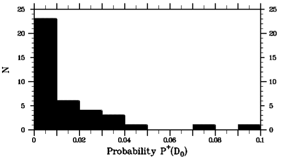
Figure 7: Distribution of the probability $P^{+}(D_{0})$ for the power density of randomized light curves to be higher than the highest values encountered in the power spectra of the real light curves for all nightly data sets.

The strong concentration of this distribution to small values of $P^{+}(D_{0})$ suggests the conclusion that the brightness variations in the light curves are not completely random. To investigate this further I consider subsequently in more detail some individual cases.

7.1.3 Individual cases

1999 June 21/22 (JD2451951):

This is the night during which Bruch et al. (Paper I ) claimed to have detected oscillations with a period of 342 sec. The light curve is shown in the upper panel of Fig. 8, while the second panel contains the pre-whitened light curve, i.e. the data after removal of the eclipses and variations on timescales above $15^{\rm m}$ as explained above. This is the light curve which was actually submitted to the power spectrum analysis. The third panel shows the power spectrum (normalized to the power density corresponding to the highest peak) with the peak at 2.92 mHz which was interpreted as being due to oscillations. In order to investigate if there is really a persistent signal at that frequency a stacked power spectrum was calculated in the following way: Sections of 1 hour duration and an overlap of 0.95 hours between successive sections were cut out of the light curve. For each of them a Lomb-Scargle periodogram was calculated and the individual power spectra were stacked on top of each other to result in the two-dimensional representation (frequency vs. time) shown in the lower panel of Fig. 8 where the grey scale varies according to power density. The frequency resolution is of the order of 0.4 mHz while in temporal direction only structures separated in time by more than 1 hour are independent.

The stacked spectra reveal that the multiple peaks in the power spectrum of the entire data set below $\approx$2 mHz can be explained by variations which persist only for a short time and occur at seemingly random frequencies. They may therefore readily be interpreted either as being due to short lived oscillations that rise rapidly and die off or become incoherent after only a few cycles, or by the accidental superposition of independent flares. The apparent oscillation at 2.92 mHz is also not caused by a persistent signal. There is only an appreciable signal at the beginning of the light curve (lower part of the stacked power spectrum). Two other events at similar frequencies appear later, separated by time spans with no signal at all. But they are not well aligned with the frequency observed in the third panel of Fig. 8. It is therefore not obvious to which degree they contribute to the peak. Even if they do it is not clear whether the repeated events occurring at similar frequencies point at some underlying physical reason or if this is just a coincidence, calling into question the interpretation given to the power spectrum in Paper I .

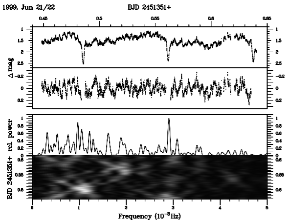
Figure 8: V893 Sco during the night of 1999 June 21/22. Top panel: Differential light curve (variable – comparison star $C_{1}$). Second panel: Same as top panel, but after removal of eclipses and variations on timescales $>$$15^{\rm m}$. Third panel: Lomb-Scargle periodogram of the light curve shown in the second panel. Lower panel: Stacked Lomb-Scargle periodograms of sliding sections of the light curve of panel two (see text for details).

2000 May 24/25 (JD2451689):

The results of the analysis of this night’s data are shown in Fig. 9 which is organized in the same way as Fig. 8. The power spectrum of the pre-whitened light curve shows a strong peak at 0.89 mHz ($P=1120^{\rm s}$). It is sufficiently outstanding to suggest that it is really due to a periodic event in the light curve. Indeed, the results obtained in Sect. 7.1.2 place this light curve among those for which $P^{+}(D_{0})=0$; i.e. in none of the power spectra of the 1 000 randomized light curves investigated in that section a peak was observed which was higher than the dominant peak corresponding to the real data.

The peak at 0.89 mHz corresponds to a period of 18${}^{\raisebox{0.90417pt}{\scriptsize m}}_{\raisebox{1.80835pt}{\hskip 1.18999pt.}}$7 which is above the nominal cut-off of $\sim$$15^{\raisebox{0.90417pt}{\scriptsize m}}$ used in the pre-whitening process. In order to investigate if it is an artefact of the data reduction the power spectrum of a light curve pre-whitened with a cut-off of $30^{\raisebox{0.90417pt}{\scriptsize m}}$ was calculated. It showed some additional features at very low frequencies, but the peak at 0.89 mHz remained unaffected, giving confidence in its reality.

The stacked power spectra show that the peak is not caused by a persistent oscillation but rather by variations which are present during about half of the duration of the observations. They not only vary in strength but also in frequency close to the frequency revealed by the power spectrum of the entire pre-whitened light curve. Although I am reluctant to exclude that the observed structure is due to a chance superposition of independent flares, variations due to a persistent but unstable physical cause appear to be more likely in this case than during the night of 1999 June 21/22, discussed above.

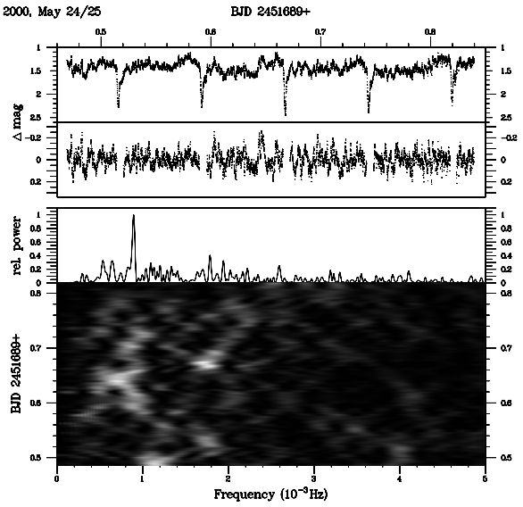
Figure 9: Same as Fig. 8, but for the night of 2000 May 24/25.

2004 July 13/14 (JD2453200):

Results for this night are shown in Fig. 10 (again, organized in the same way as Fig. 8). Similar to the night of 2000 May 24/25, the power spectrum of the pre-whitened data has a strongly dominant peak at 0.86 mHz ($P=1168^{\rm s}$) which suggests some kind of persistent oscillation in the light curve. Also in this case $P^{+}(D_{0})=0$ was found in Sect. 7.1.2. The peak corresponding to a period longer than the nominal pre-whitening cut-off, as in the previous example a power spectrum calculated after a pre-whitening with a cut-off of $30^{\raisebox{0.90417pt}{\scriptsize m}}$ showed that is is not an artefact of the data reductions. In contrast to the other examples discussed in more detail in this section, V893 Sco was observed during this night in a somewhat lower photometric state than normal quiescence, as mentioned in Sect. 3. Contrary to all other observations there is no indication of an orbital hump during this low state, suggesting that no light modulation due to a variable visibility (or the presence) of a bright spot occurs. Moreover, the overall variability of V893 Sco on timescales less than $15^{\rm m}$ is higher during this night as revealed by the increased amplitude of variations in the pre-whitened light curve.

The stacked power spectra show a signal which, while not perfectly stable in strength over time and in frequency, persist over most of the duration of the light curve. Of all the examples investigated so far I consider this the most convincing of a signal which cannot easily be explained by a chance superposition of independent flares. It is also noteworthy that the frequency of 0.86 mHz is close to the that observed on 2000 May 24/25 (0.89 mHz). Moreover, apart from a particularly strong event at $\approx 1$ mHz close to the end of the light curve (upper part of the stacked power spectrum) there appears to be a parallel sequence close to $\approx 1.35$ mHz at least during a part of the observations (which does not show up prominently in the power spectrum of the pre-whitened light curve). Without trying any interpretation I mention that the ratio of the two frequencies is close to 2/3.

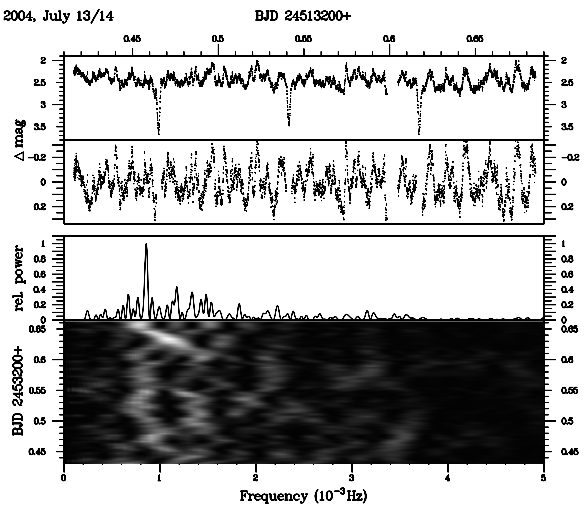
Figure 10: Same as Fig. 8, but for the night of 2004 July 13/14.

2000 June 6/7 (JD2451702):

Finally, the results of the night of 2000 June 6/7 (Fig. 11) are included as an example of a light curve which does not exhibit any indication of a persistent oscillation. The power spectrum of the pre-whitened data contain a multitude of unrelated peaks between 0.5 mHz and 2.5 mHz. But none of them is in any way outstanding or suggests a significant signal. While the distribution of structures in the stacked power spectra is not completely at random, in contrast to other nights it does not suggest the presence of anything which cannot be explained by stochastic variations in the light curve.

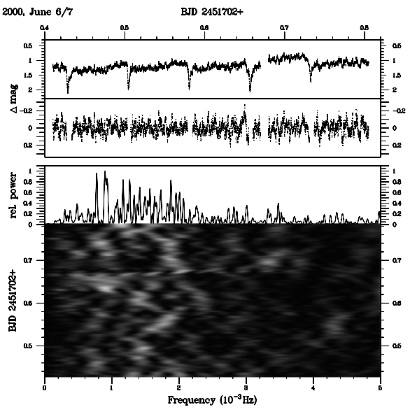
Figure 11: Same as Fig. 8, but for the night of 2000 June 6/7.

This

small sample of individual cases should be sufficient to characterize in a general way the occurrence of apparent or real oscillations in the light curves of V893 Sco. The power spectra of the pre-whitened light curves from the nights not discussed here all range between the extreme cases of apparently significant signals such as on the night of 2004 Jul 13/14, or apparently random signals as exemplified by the data of 2000 June 6/7. In the ensemble of data which permit to nurture the suspicion of a real signal no preference of a particular frequency other than the general and wide range of 0.5 - 3 mHz can be found.

7.2 High and low frequencies

At high frequencies (periods shorter that $2^{\rm m}$) the power spectra of the pre-whitened light curves did not suggest the presence of oscillations in any of the nightly data sets. In order to investigate if short lived periodicities hide in the data which do not reveal themselves in a analysis of the complete light curves, stacked power spectra, using sections of 900 sec duration with an overlap of 864 sec between successive sections were calculated. They also did not reveal any structures which cannot be explained by short lived random brightness fluctuations. Their amplitudes decrease with increasing frequency as is typical for flickering (Bruch Bruch92 (1992)). In particular, no signal which could convincingly be interpreted as being due to DNOs was found in the light curve of 2002 May 15/16, the only one which was observed during (the decline from) an outburst and thus at a phase when DNOs are most often seen in other dwarf novae (Would & Warner, Would (2002)).

Not surprisingly, variations in the low frequency range (periods $>$$15^{\rm m}$) are dominated by the orbital frequency. Analysing this range, no pre-whitening of the light curves was performed, but the eclipses were masked. The power spectra of all data sets of sufficient length have a strong peak close to $f_{\rm orb}=0.55$/hour, corresponding to the binary period, in most cases accompanied by a smaller peak at twice this value, i.e. the first overtone of the orbital frequency. Sometimes signals at lower frequencies also occur, caused by variations on timescales longer than the revolution period of V893 Sco. They do not represent real periodicities as is evident from the fact that their frequencies are not repeatable. A good example is shown in Fig. 12 where the upper frame contains the light curve of 2000 June 9/10, and the lower frame the low frequency part of the corresponding power spectrum. The peaks corresponding to the orbital frequency and its first harmonic are somewhat offset from their nominal values, marked by dashed vertical lines. This can easily be explained by the strong variability of the features (hot spot and possibly other structure in the accretion disk) causing these signals and by the small number of cycles covered by the light curve. The solid curve in the upper frame is a 4-term least squares sine fit (after masking the eclipses) to the data with periods fixed to values corresponding to the four dominating peaks in the power spectrum.

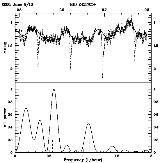
Figure 12: Top Differential light curve of V893 Sco of the night of 2000 June 9/10. Bottom: Low frequency part of the power spectrum of the light curve, after masking the eclipses. The orbital frequency and its first harmonic are marked by dashed vertical lines. The solid line in the upper frame is a 4 term sine fit (eclipses masked) with periods fixed to the values corresponding to the dominant peaks in the power spectrum.

On some occasions light curves were observed during several subsequent nights (or with a gap of only one night between them). The power spectra of the combined data sets should reveal periodic variations on timescales significantly longer than the orbital period if they exist. However, no consistent long-term fluctuations were found.

8 Conclusions

I have presented results of a long-term photometric study of the eclipsing dwarf nova V893 Sco, focussing on a new determination of the eclipse ephemerides and their interpretation, and on possible oscillations in the brightness of the system. The main conclusions can be summarized as follows:

1. Normal outbursts with a comparatively low amplitude are frequent but the absence of superoutbursts during 13 years of monitoring is unusual for a dwarf nova with a period below the gap in the orbital period distribution of cataclysmic variables. The likelihood for superoutbursts to hide in the observational gaps is found to be small, unless the supercycle is close to one year (or multiples thereof) and all superoutburst occur around conjunction of V893 Sco with the sun.

2. The eclipse profile is strongly variable in shape, amplitude and minimum magnitude. Large differences in the visibility of the bright spot in the profiles of individual eclipses show that it is outshone by the strong ubiquitous flickering. On average, about 36% of the total light of V893 Sco is occulted during mid-eclipse.

3. Updated orbital ephemerides are calculated from eclipse timings, leading to a significantly more precise value of the orbital period. Simple linear ephemerides cannot adequately describe the observations. While a quadratic term is not significant, the orbital period undergoes a cyclic variation which leads to a sinusoidal modulation of 22.3 sec in the $O-C$ diagram with a period of 10.2 years.

4. These cyclic variations can be interpreted as a light travel time effect if the presence of a giant planet with a mass of the order of 9.5 Jupiter masses at a distance of 4.5 AU from the binary system is postulated. It was shown that a planet with these characteristics can survive the common envelope phase which must have preceded the appearance of V893 Sco as a CV if the mass of the white dwarf in the system is on the low side of the distribution of white dwarf masses in cataclysmic variables ($\approx 0.5-0.6\,M_{\sun}$).

5. A search for oscillations in the light curves of V893 Sco was performed. At low frequencies, no persistent signal other than a modulation with the orbital period and its first harmonic was detected. At high frequencies a search of DNO-type oscillations met with no success. More interesting and also more difficult to interpret are oscillations at intermediate frequencies (timescale: $2^{\rm m}\leq\tau\leq 15^{\rm m}$). In some light curves transient oscillations at frequencies between 0.5 and 3 mHz are seen for part of the time which may be identified with QPOs. However, an accidental superposition of unrelated flickering flares may also lead to the observed signals. Simulations were performed in order to gain insight to which degree random fluctuation can mimic QPOs. To this end randomized version of real light curves were analysed. It was shown that in a non-negligible fraction of cases their power spectra contained signals which can be mistaken as being due to QPOs. The simple detection of an apparently significant signal in the power spectrum of a light curve containing strong flickering is therefore not sufficient to claim the presence of QPOs. Even so, it is shown to be unlikely that all apparent oscillations seen in the present ensemble of light curves can be explained by a chance superposition of unrelated events. Therefore at least some of them must have a physical origin. The question to which degree QPOs and flickering are really conceptually different is raised.

- (1) Applegate, J.H. 1992, ApJ, 385, 621
- (2) Bessell, M.S. 1990, PASP, 102, 1181
- (3) Beuermann, K., Breitenstein, P., Debski, et al. 2012a, A&A, 540, A8
- (4) Beuermann, K., Buhlmann, J., Diese, J., et al. 2011, A&A, 526, A53
- (5) Beuermann, K., Dreizler, S., Hessman, F.V., & Deller, J. 2012b, A&A, 543, A138
- (6) Beuermann, K., Hessman, F.V., Dreizler, S., et al. 2010, A&A, 521, L60
- (7) Bobinger, A., Barwig, H., Fiedler, H., et al. 1999, MNRAS, 348, 145
- (8) Borges, B.W., Baptista, R., Papadimitriou, C., & Giannakis, O. 2008, A&A, 480, 481
- (9) Brinkworth, C.S., Marsh, T.R., Dhillon, V.S., & Knigge, C. 2006, MNRAS, 365, 287
- (10) Bruch, A. 1992, A&A, 266, 237
- (11) Bruch, A. 1993, MIRA: A Reference Guide (Astron. Inst. Univ. Münster)
- (12) Bruch, A. 1996, A&A, 312, 97
- (13) Bruch, A. 2000, A&A, 359, 998
- (14) Bruch, A., Steiner, J.E., & Gneiding, C.D. 2000, PASP, 112, 237 (Paper I)
- (15) Caceci, M.S., & Cacheris, W.P. 1984, Byte, May 1984, 340
- (16) Catalán, S., Isern, J., García-Berro, E., & Ribas, I. 2008, MNRAS, 387, 1693
- (17) Dai, Z.B., & Qian, S.B. 2009, A&A, 503, 883
- (18) Dai, Z., Qian, S., & Fernández Lajús, E. 2009, ApJ, 703, 109
- (19) Dai, Z., & Qian, S. 2010, New A, 15 , 380
- (20) Dai, Z., Qian, S., Fernández Lajús, E., & Baume, G.L. 2010, Ap&SS, 330, 243
- (21) Eastman, J., Siverd, R., & Gaudi, B.S. 2010 PASP, 122, 935
- (22) Goździewski K., Nasiroglu I., Słowikowska A., et al. 2012, MNRAS, 425, 930
- (23) Hessman F.V., Beuermann K., Dreizler S., et al. 2011, AIP Conf. Proc., 1331, 281
- (24) Holman, M.J., & Wiegert, P.A. 1999, AJ, 117, 623
- (25) Horne, J.H., & Baliunas, S.L. 1986, ApJ, 302, 757
- (26) Horner, J., Marshall, J.P., Wittemyer, R.A., & Tinney, C.G. 2011, MNRAS, 416, L11
- (27) Horner, J., Hinse, T.C., Wittenmyer, R.A., Marshall, J.P., & Tinney, C.G. 2012, MNRAS, 427, 2812
- (28) Howell, S.B., & Skidmore, W. 2001, NewA Rev., 44,33
- (29) Irwin, J.B. 1952, ApJ, 116, 211
- (30) Joss, P.R., Rappaport, S., & Lewis, W. 1987, ApJ, 319, 180
- (31) Kato, T., Haseda, K., Takamizawa, K., Kazarovets, E.V., & Samus, N.N. 1998, Inf. Bull. Variable Stars, 4585, 1
- (32) Kato, T., Hambsch, F.-J., Uemura, M., et al. 2013, PASJ, 65, 23
- (33) Kato, T., Imada, A., Uemura, M., et al. 2009, PASJ, 61, S395
- (34) Kato, T., Maehara, H., Miller, I., et al. 2012, PASJ, 64, 21
- (35) Kato, T., Maehara, H., Uemura, M., et al. 2010, PASJ, 62, 1525
- (36) Knigge, C. 2006, MNRAS, 373, 484
- (37) Knigge, C., Baraffe, I., & Patterson, J. 2011, ApJS, 194, 28
- (38) Lanza, A.F., Rodonó, M., & Rosner, R. 1998, MNRAS, 296, 893
- (39) Lee J.W., Kim S.-L., Kim C.-H., et al. 2009, AJ, 137 3181
- (40) Lomb, N.R. 1976, Ap&SS, 39, 447
- (41) Mason, E., Skidmore, W., Howell, S.B., & Mennickent, R.E. 2001, ApJ, 563, 351
- (42) Matsumoto, K., Mennickent, R.E., & Kato, T. 2000, A&A, 363, 1029
- (43) Mukai, K., Zietsman, E., & Still, M. 2009 ApJ, 707, 652
- (44) Marsh T.R., Parsons S.G., Bours M.C.P., et al. 2014, MNRAS, 437, 475
- (45) Nordhaus, J., & Spiegel, D.S. 2013, MNRAS, 432, 500
- (46) Pilarčík, L., Wolf, M., Dubovský, P.A., Hornoch, K., & Kotková, L. 2012, A&A, 539, A139
- (47) Parsons, S.G., Marsh, T.R., Copperwheat, C.M., et al. 2010, MNRAS, 407, 2362
- (48) Patterson, J., 1984, ApJS, 54, 443
- (49) Potter, S.B., Romero-Colmenero, E., Ramsay, G., et al. 2011, MNRAS, 416, 2202
- (50) Pretorius, M.L., Warner, B., & Woudt, P.A. 2006, MNRAS, 368, 361
- (51) Qian S.-B., Dai Z.-B., He J.-J., et al. 2007, A&A, 466, 589
- (52) Qian S.-B., Dai Z.-B., Liao W.P., et al. 2009, ApJ, 706, L96
- (53) Qian, S.-B., Liao, W.-P., Zhu, L.-Y., & Dai, Z.-B. 2010a, ApJ, 708, L66
- (54) Qian, S.-B., Liao, W.-P., Zhu, L.-Y., et al. 2010b, MNRAS, 401, L34
- (55) Qian, S.-B., Liu, L., Liao, W.-P., et al. 2011, MNRAS, 414, L16
- (56) Qian, S.-B., Liu, L., Zhu, L.-Y., et al. 2012, MNRAS, 422, L24
- (57) Salaris, M., Serenelli, A., Weiss, A., & Miller Bertolami, M. 2009, ApJ, 692, 1013
- (58) Satyvoldiev, V. 1972, Astron. Tsirk., 711, 1
- (59) Scargle, J.D. 1982, ApJ, 263, 853
- (60) Thorstensen, J.R. 2003, AJ, 126, 3017
- (61) Warner, B., 1995, Cataclysmic Variable Stars. Cambridge University Press
- (62) Warner, B. 2004, PASP, 116, 115
- (63) Warner, B., Woudt, P.A. & Pretorius, M.L. 2003, MNRAS, 344, 1193
- (64) Wittenmyer, R.A., Horner, J., Marshall, P.J., Butters, O.W., & Tinney, C.G. 2012, MNRAS, 419, 3258
- (65) Wood, J.H., Horne, K., Berriman, G., & Wade, R.A. 1989, ApJ, 341, 974
- (66) Wood, J.H., Horne K., Berriman G., et al. 1986, MNRAS, 219, 629
- (67) Wood, M.A., & Burke C.J. 2007, ApJ, 661, 1042
- (68) Would, P.A., Warner, B. 2002, MNRAS, 333, 411
- (69) Zhao, J.K., Oswalt, T.D., Willson, L.A., Wang, Q., & Zhao, G. 2012, ApJ, 746, 144
- (70) Zharikov, S., Tovmassian, G., Aviles, A., et al. 2013, A&A, 549, A77
- (71) Zacharias, N., Urban, S.E., Zacharias, M.I., et al. 2004 AJ, 127, 3043
- (72) Zorotovic, M., & Schreiber, M.R. 2013, A&A, 549, A95