Efficiency at optimal work from finite reservoirs:
a probabilistic perspective

Abstract

We revisit the classic thermodynamic problem of maximum work extraction from two arbitrary sized hot and cold reservoirs, modelled as perfect gases. Assuming ignorance about the extent to which the process has advanced, which implies an ignorance about the final temperatures, we quantify the prior information about the process and assign a prior distribution to the unknown temperature(s). This requires that we also take into account the temperature values which are regarded to be unphysical in the standard theory, as they lead to a contradiction with the physical laws. Instead in our formulation, such values appear to be consistent with the given prior information and hence are included in the inference. We derive estimates of the efficiency at optimal work from the expected values of the final temperatures, and show that these values match with the exact expressions in the limit when any one of the reservoirs is very large compared to the other. For other relative sizes of the reservoirs, we suggest a weighting procedure over the estimates from two valid inference procedures, that generalizes the procedure suggested earlier in [J. Phys. A: Math. Theor. 46, 365002 (2013)]. Thus a mean estimate for efficiency is obtained which agrees with the optimal performance to a high accuracy.

1 Introduction

Maximum work extraction is a well-known problem in classical thermodynamics [1, 2, 3, 4, 5, 6]. It is known that an entropy preserving process yields the upper bound for work. In recent years, the field of finite-time thermodynamics has been intensely investigated, where the power output per cycle is often sought to be maximum [7, 8]. Related to these considerations, the efficiency of engines at maximum work or power has caught attention, in particular, the discussion about its universality near equilibrium.

In this paper, we consider the issue of efficiency at maximum work [4, 9] from an entirely different, probabilistic standpoint. Rather than performing an optimization of the extracted work, our approach follows inductive reasoning or inference [10, 11, 12]. The latter has served as a powerful tool in situations with incomplete information and is increasingly being applied to the analysis of a wide range of phenomena, such as in particle physics [13], cosmology [14], artificial intelligence [15, 16] and so on.

The approach is based on the subjective or Bayesian viewpoint [17, 18, 19] according to which probabilities denote the degree of rational belief or the state of knowledge of an agent. The knowledge which is available before any data is gathered, is called the prior information and the degree of belief about the possible values taken by a parameter is encapsulated in a prior probability function [20]. The basic idea of estimating from prior information was first proposed in [22], in the context of quantum thermodynamic machines and later extended to treat uncertainty in other thermodynamic processes in Refs. [24, 25, 26, 27]. A remarkable result of these studies is that even with the treatment of uncertainty in a subjective sense, the analysis affords reliable estimates of quantities such as maximum work as well as the efficiency at maximum work.

In view of the correspondence achieved between the optimal results and the inference based approach, it seems of importance to extend the approach to more general situations. In this paper, a generalization of Refs. [25, 27] is presented which considers the similar problem but with arbitrary sizes of reservoirs. Recalling the approach, the central issue was the assignment of the prior in a constrained thermodynamic process, for the uncertain variable such as the temperature. For the case of identical reservoirs which differ only in their temperatures, we treated the invariance of the prior as the basis for the assignment. The extension presented in this paper assigns priors by taking into account the differences in the reservoirs, prescribed in the prior information. For simplicity of analysis, we illlustrate the approach using only the perfect gas model for the reservoirs.

2 Efficiency at optimal work

Consider two perfect gas reservoirs of constant heat capacities $C_{1}$ and $C_{2}$. Let they be at initial temperatures $T_{+}$ and $T_{-}<T_{+}$. The maximum work is extracted by removing, in a quasi-static manner, a small amount of heat from the hot reservoir, converting it to work with the maximal efficiency, while discarding the waste heat to the cold reservoir. Thus in a sequence of infinitesimal cycles, the temperatures of the two reservoirs slowly approach each other. The process terminates and is said to be optimal when the reservoirs achieve a common temperature.

We consider an arbitrary intermediate state of this process, when the temperatures are $T_{i}^{\prime}$, $i=1,2$. The work extracted upto this stage is:

$$W=C_{1}T_{+}+C_{2}T_{-}-C_{1}T_{1}^{\prime}-C_{2}T_{2}^{\prime},$$ (1)

where $W>0$. For convenience, we define $C_{2}/C_{1}=x$, $T_{-}/T_{+}=\theta$, $T_{1}=T_{1}^{\prime}/T_{+}$ and $T_{2}=T_{2}^{\prime}/T_{+}$. So the work is rewritten as $W=C_{1}T_{+}(1+x\theta-T_{1}-xT_{2}).$ The constraint of entropy conservation for perfect gases: $\Delta S=C_{1}\ln T_{1}+C_{2}\ln T_{2}-C_{1}\ln T_{+}-C_{2}\ln T_{-}=0,$ yields the following one-to-one relation between the two scaled temperatures:

$$T_{1}=\theta^{x}{T_{2}}^{-x}.$$ (2)

For the optimal process, the final common temperature is $T_{c}=\theta^{x/1+x}$. The efficiency at optimal work (distinguished by a cap) is:

$${\hat{\eta}}_{\rm op}=1-\frac{x(\theta^{x/1+x}-\theta)}{(1-\theta^{x/1+x})}.$$ (3)

It is also of interest to consider efficiency for intermediate stages. First, we can use Eq. (2) to express $W$ as a function of one variable only, such as

$$W(T_{2})=C_{1}T_{+}\left(1+x\theta-\theta^{x}{T_{2}}^{-x}-xT_{2}\right),$$ (4)

where $\{C_{1},T_{+},x,\theta\}$ all are fixed for the given process. One can distinguish two regimes:

a) $x<1$: In this case, it is convenient to express efficiency in terms of the variable $T_{2}$. Thus the heat going “into” and the heat going “out” of the engine is given as

$$Q_{\rm in} = C_{1}T_{+}(1-T_{1}),$$ (5)

$$= C_{1}T_{+}\left(1-\theta^{x}{T_{2}}^{-x}\right),$$ (6)

$$Q_{\rm out} = C_{2}T_{+}(T_{2}-\theta).$$ (7)

The efficiency defined by $\eta_{x}=1-{Q_{\rm out}}/{Q_{\rm in}}$, is given as

$$\eta_{x}=1-\frac{x(T_{2}-\theta)}{\left(1-\theta^{x}{T_{2}}^{-x}\right)}.$$ (8)

In particular, in the limit $x\to 0$, i.e. when the hot reservoir is very large compared to the cold one, the efficiency becomes

$$\eta_{0}=1+\frac{T_{2}-\theta}{\ln\left({\theta}/{T_{2}}\right)}.$$ (9)

Also in this limit, the temperature of the hot reservoir is assumed to stay constant at $T_{1}^{\prime}=T_{+}$, or $T_{1}=1$. Then for the optimal work extraction, the temperature of the cold reservoir must approach this value. Thus substituting $T_{2}=1$ in Eq. (9), we obtain

$${\hat{\eta}}_{0}=1+\frac{(1-\theta)}{\ln\theta}.$$ (10)

b) $x>1$: For this case, it is convenient to use $T_{1}$ as the variable. From Eqs. (2) and (4), we have

$$W(T_{1})=C_{1}T_{+}(1+x\theta-T_{1}-x\theta{T_{1}}^{-1/x}),$$ (11)

with the efficiency rewrtitten as

$$\eta_{x}=1-\frac{x\theta({T_{1}}^{-1/x}-1)}{\left(1-T_{1}\right)}.$$ (12)

In the limit $x\to\infty$,

$$\eta_{\infty}=1+\frac{\theta\ln T_{1}}{(1-T_{1})}.$$ (13)

This applies to a very large cold reservoir in comparison to a finite hot reservoir. Here the temperature of the cold reservoir does not change i.e. remains at $T_{-}$. For the optimal process, the temperature of the other reservoir must approach this value. So substituting $T_{1}^{\prime}=T_{-}$ or $T_{1}=\theta$ in Eq. (13), we obtain the efficiency

$${\hat{\eta}}_{\infty}=1+\frac{\theta\ln\theta}{(1-\theta)}.$$ (14)

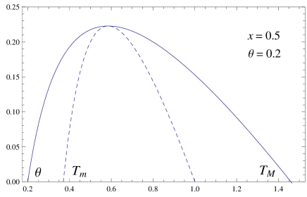
Figure 1: Work expressions, Eqs. (4) and (11), plotted versus the relevant temperature, as solid and dashed curves respectively, for $W\geq 0$. For $x<1$, the interval $[T_{m},1]$ of the allowed $T_{1}$ values, is smaller than the corresponding interval $[\theta,T_{M}]$ for $T_{2}$.

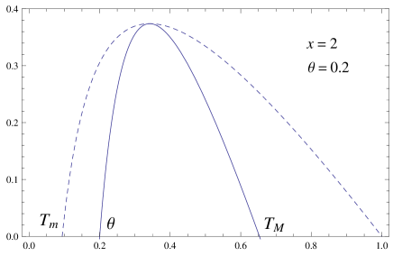
Figure 2: Work expressions plotted versus temperature, as in Fig. 1, here for $x=2$. For $x>1$, the interval of $T_{2}$ values is smaller than the allowed interval for $T_{1}$.

It was observed in [4] that the efficiency at optimal work is rather insenstive to the relative sizes of the reservoirs. For most temperature ranges, it is well approximated by the expression: $1-\sqrt{\theta}$. We have considered two limiting cases, when one of the reservoirs is very large compared to the other. Then near equilibrium, i.e. for $\theta$ close to unity, the efficiency at maximum work, behaves as $(1-\theta)/2$.

3 Inference

In this section, we approach the issue of efficiency at optimal work from the perspective of inference. The main approach has been elaborated in Refs. [25, 27]. Here our purpose is to seek a generalization for different sized reservoirs.

3.1 Prior information

It is instructive to consider the graphical form of Eqs. (4) and (11), as shown in Figs. 1 and 2 for different $x$ values. In particular, as in Fig. 1 for $x<1$, i.e. for a small cold reservoir and larger hot reservoir, the range of $T_{1}$ values satisfying $W\geq 0$ (dashed curve), is narrower than the range of $T_{2}$ values (solid curve). The two intervals are respectively given as $[T_{m},1]$ and $[\theta,T_{M}]$. Due to Eq. (2), we have $T_{m}=\theta^{x}{T_{M}}^{-x}$. For $x=1$, the two intervals are identical to $[\theta,1]$. Further, following Fig. 1, as $x$ approaches zero, the range $[T_{m},1]$ shrinks because $T_{m}\to 1$, meaning that as the hot reservoir becomes very large, its temperature tends to remain at its initial value. Similarly, we can extrapolate from Fig. 2 that as $x\to\infty$, $T_{M}\to\theta$.

Now imagine a situation where we are ignorant of the final values $T_{1}$ and $T_{2}$. We adopt the Bayesian approach proposed in [25, 27] to deal with this uncertainty. In this approach, we first clearly identify the prior information that we possess on the system:

(i) Whatever the values of $T_{1}$ and $T_{2}$, these satisfy a one-to-one relation, Eq. (2).

ii) Due to condition (i), there is essentially one variable in the problem, and so an observer is free to formulate the problem in terms of either $T_{1}$ or $T_{2}$.

(iii) Even when an observer is ignorant of the exact values of temperatures, his/her state of knowledge regarding the true value $T_{1}$, is the same as the state of an equivalent observer with respect to $T_{2}$.

(iv) An observer possesses knowledge of the function $W(T_{1})$ or equivalently of $W(T_{2})$, with the condition $W\geq 0$. In the physical context, it means the set-up works like a heat engine.

The first implication of the condition $W\geq 0$, is that it fixes the intervals of possible values for the variables $T_{1}$ and $T_{2}$, as shown in Figs. 1 and 2. It should be emphasized that in our approach, we also include the temperature values otherwise deemed unphysical in the standard thermodynamic treatment (see Fig. 3). The interval of possible values is decided solely by the form of the function $W$ alongwith the condition $W\geq 0$.

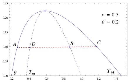
Figure 3: Work versus temperature $T_{1}$ (longdashed curve) and $T_{2}$ (solid curve). For a given value of the work extracted (horizontal dashed line), there are two possible values each, of $T_{2}$ (abcissae of points $A$ and $C$) and of $T_{1}$ (abcissae of $B$ and $D$). Only the temperature values corresponding to $A$ and $B$ are considered physical, because they satisfy the inequality $T_{2}<T_{1}$ and accord with the natural tendency of heat flow from “hot to cold”. The other value of $T_{2}$ (for the point $C$) and the corresponding value of $T_{1}$ (point $D$) do not satisfy this order, and usually are disregarded for being unphysical.

To close this section, we have considered two observers, one of whom interprets the uncertainty in terms of variable $T_{2}$ while the other, in terms of $T_{1}$. Each observer must now quantify the prior information at his/her command, by assigning prior probabilities for the likely values of the relevant temperature.

3.2 The prior and the estimates

Further, in view of the points (ii) and (iii) above, the problem of the choice of a prior distribution function by either observer seems to be equivalent. So for consistency, the same form of the prior distribution function would be assigned for each case. Moreover, the one-to-one relation between a pair of values $(T_{1},T_{2})$ suggests that the probability of $T_{1}$ to lie in a small range $[T_{1},T_{1}+dT_{1}]$ is the same as the probability of $T_{2}$ to lie in $[T_{2},T_{2}+dT_{2}]$, where the particular values of $T_{1}$ and $T_{2}$ are related by Eq. (2). Thus we require that

$$\pi_{1}(T_{m}\leq T_{1}\leq 1)dT_{1}=\pi_{2}(\theta\leq T_{2}\leq T_{M})dT_{2},$$ (15)

where $\pi_{i}$ is a (normalizable) prior distribution function. Equivalently, in terms a function $f$, yet to be assigned, the above condition is rewritten as

$$\frac{f(T_{1})}{\int_{T_{m}}^{1}f(T_{1})dT_{1}}\left|\frac{dT_{1}}{dT_{2}}\right|=\frac{f(T_{2})}{\int_{\theta}^{T_{M}}f(T_{2})dT_{2}}.$$ (16)

Finally, the use of Eq. (2) in the above, straightforwardly leads to the form of the prior, by fixing $f(T)=1/T$.

Thus for instance, the state of knowledge of observer 2, is expressed by the prior:

$$\pi_{2}(T_{2})=\frac{{T_{2}}^{-1}}{\ln({T_{M}}/{\theta})},$$ (17)

which gives an expected value of

$$\overline{T}_{2}=\frac{(T_{M}-\theta)}{\ln({T_{M}}/\theta)}.$$ (18)

The estimate for maximum work according to observer 2, is given by $W(\overline{T}_{2})$ [25]. Thereby, the efficiency at maximum work is given by replacing $T_{2}\to\overline{T}_{2}$ in Eq. (8):

$${\tilde{\eta}}_{x}=1-\frac{x(\overline{T}_{2}-\theta)}{\left(1-\theta^{x}{\overline{T}_{2}}^{-x}\right)}.$$ (19)

For the behavior of this efficiency near equilibrium, see the Appendix.

For general $x$ values, the value $T_{M}$ is determined by numerically solving the equation $W(T_{2})=0$, Eq. (4), which implies solving

$$\frac{\theta}{T_{2}}=[1+x(\theta-T_{2})]^{1/x},$$ (20)

whose trivial solution is $T_{2}=\theta$. The other solution is evaluated numerically. In the special case of $x\to 0$, the rhs of Eq. (20) becomes an exponential function. In this limit, $T_{M}$ is a solution of

$$T_{M}\exp(-T_{M})=\theta\exp(-\theta).$$ (21)

It is directly verified that Eqs. (18) and (21) together imply that the expected value $\overline{T}_{2}=1$. Thus for $x\to 0$, the average estimate of $T_{2}$ infers exactly the optimal process discussed in Section II, and the estimate for efficiency is the same as Eq. (10). Again in this limit, the range $[T_{m},1]$ of $T_{1}$, shrinks to zero and so only the inference on temperature $T_{2}$, needs to be conducted.

Similarly, the corresponding prior for $T_{1}$, is

$$\pi_{1}(T_{1})=\frac{{T_{1}}^{-1}}{\ln(1/{T_{m}})},$$ (22)

with the expected value

$$\overline{T}_{1}=\frac{(1-T_{m})}{\ln(1/{T_{m}})}.$$ (23)

Again, the estimate for efficiency at maximum work in terms of temperature $T_{1}$, is to be obtained by replacing $T_{1}$ by $\overline{T}_{1}$ in Eq. (12).

For general $x$ values, the value $T_{m}$ is determined by numerically solving the equation $W(T_{1})=0$. For the limit $x\to\infty$, $T_{m}$ is the solution of

$$T_{m}\exp(-T_{m}/\theta)=\exp(-1/\theta).$$ (24)

whose trivial solution is $T_{m}=\theta$. It can be seen that Eqs. (23) and (24), together imply that $\overline{T}_{1}=\theta$. So for this case also, we infer an optimal process from the average estimate for $T_{1}$. The estimate for efficiency is the same as $\eta_{\infty}$ in Eq. (13). Again, in this limit, only the inference on $T_{1}$ is to be performed, as the other temperature remains fixed.

4 Estimates with arbitrary $x$

We have seen that when one of the reservoirs is very large compared to the other, the estimates for efficiency at optimal work correspond exactly to the values obtained by direct optimization of work. It is then of interest to see how the estimates of efficiency compare with the optimal values for arbitrary values of $x$. In Figs. 4 and 5, we show the estimates made by observer 1 and 2, for different $x$ values. Apparently, the estimates by the two observers match with the optimal values when close to equilibrium ($\theta\approx 1$). Further, for $x<1$, the estimates in terms of $T_{2}$ lie closer to the optimal value, the agreement being exact in the limit $x\to 0$. Similarly, for $x>1$, the agreement between the optimal behavior and the estimate by observer 1 is better, whereby the agreement becomes exact for $x\to\infty$.

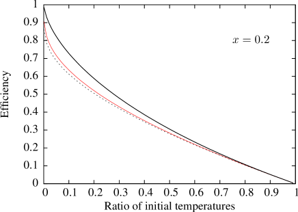
Figure 4: Efficiency versus ration of initial temperatures, $\theta$. Upper curve is the estimated efficiency at optimal work due to an observer using $T_{1}$ as the variable, the lower curve corresponds to an observer using $T_{2}$ variable. The middle curve (red online) is the efficiency at optimal work, Eq. (3). Note that for $x<1$, the latter is closer to the estimate by observer 2.

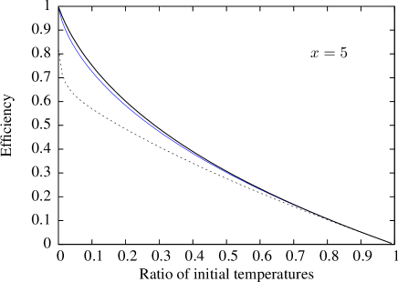
Figure 5: Upper curve is the estimated efficiency at optimal work using $T_{1}$ variable, the lower curve corresponds to use of $T_{2}$ variable. The middle curve (blue online) is the efficiency at optimal work and is closer to the estimate of observer 1, when $x>1$.

Close to equilibrium, the efficiency at optimal work for arbitrary $x$, Eq. (3) behaves as:

$$\hat{\eta}_{\rm op}=\frac{\eta_{c}}{2}+\frac{(1+2x)}{12(1+x)}\eta_{c}^{2}+O[\eta_{c}^{3}]+\cdots$$ (25)

In this regime, the estimates from each observer behave as folllows (see Appendix)

$$\tilde{\eta}_{2} = \frac{\eta_{c}}{2}+\frac{\eta_{c}^{2}}{12}+O[{\eta_{c}^{3}}]+\cdots$$ (26)

$$\tilde{\eta}_{1} = \frac{\eta_{c}}{2}+\frac{\eta_{c}^{2}}{6}+O[{\eta_{c}^{3}}]+\cdots$$ (27)

These considerations motivate the observation that the efficiency at optimal work for arbitrary $x$, can be estimated as a weighted mean over the estimates due to each observer. In fact, let the mean estimate of efficiency at optimal work, be defined as

$$\tilde{\eta}=\frac{x}{1+x}\tilde{\eta}_{2}+\frac{1}{1+x}\tilde{\eta}_{1}.$$ (28)

This definition is consistent with the exact agreement observed for the limiting cases discussed in previous sections. Further, the agreement with the efficiency at optimal work upto second order, Eq. (25), is also obtained. The complete expression, Eq. (3) is plotted in Fig. 6 and compared with the weighted estimate, Eq. (28). The case of equal sized reservoirs implies equal weights of one-half each, which has been discussed in [25, 27].

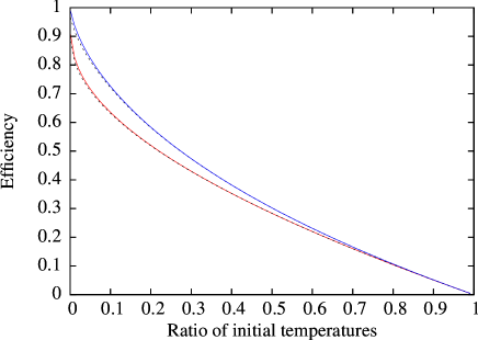
Figure 6: The lower curve (red online) for $x=0.2$ and the upper curve (blue online) for $x=5$, represent efficiency at optimal work as in Figs. 4 and 5. The dashed curves closely following the above curves are obtained by weighing the two estimates of efficiency, as given by Eq. (28).

5 Conclusion

Motivated by earlier findings, in which the Bayesian prior probabilities were used to infer the optimal performance characteristics of heat engines and other processes, in this paper we have attempted to extend this approach to the scenario of different-sized reservoirs. Using perfect gases as the reservoirs, we have reasoned the appropriate prior which is a renormalised version of the earlier one derived for similar-sized reservoirs. The main focus of this paper is the estimation of efficiency at optimal work. It has been shown that the estimates of the said efficiency are exact in the limiting cases of one reservoir being very large compared to the other. For intermediate cases, a mean estimate for efficiency may be defined, which reproduces the optimal value close to equilibrium, correct upto second order of the carnot efficiency.

The present generalization further emphasizes the relevance of prior information in the success of the inferential approach. Now the information on different sizes of the reservoirs, distinguishes the two temperatures and assigns each to a specific reservoir. In our case, $T_{1}$ has been assigned to the reservoir with heat capacity $C_{1}$ or to the one that was initially hotter ($T_{+}$). Note that this information was missing in earlier studies where similar-sized reservoirs were considered.

Further, due to difference in the sizes, the intervals of possible values for $T_{1}$ and $T_{2}$, consistent with the physical condition of work extraction $W\geq 0$, are now different. Clearly, the intervals reduce to the common interval $[\theta,1]$ for similar sizes of the reservoirs. As discussed in Fig. 3, the inferred interval of allowed values, includes values which are not considered in the physical model. In particular, the spontaneous flow of heat dictates that the initially hot reservoir remains hotter than the other, initially cold reservoir. In this sense, the inference based analysis is more abstract and does not make use of all the physical considerations relevant to the actual process. This aspect reminds one of Jaynes’ approach to statistical mechanics where the latter is looked upon as a theory of statistical inference and physical considerations of ensembles, reservoirs are not necessary for inferring the state of the system consistent with the given prior information.

Appendix

In the following, we derive the estimates for efficiency when $\theta$ is close to unity, so that $\eta_{c}=1-\theta$ is a small parameter. For convenience, we take $0<x<1$. Refering to Fig. 1, when the lower bound $\theta$ for $T_{2}$, is close to unity, the upper bound $T_{M}>1$, is also close to unity. Introducing the small parameter $\omega>0$ as $T_{M}/\theta=1+\omega$, we can rewrite Eq. (20) as $1-(1-\eta_{c})x\omega=(1+\omega)^{-x}$. Applying binomial expansion to the rhs of this equation, we obtain upto second order:

$$(1+x)(2+x)\omega^{2}-3(1+x)\omega+6\eta_{c}=0,$$ (29)

whose acceptable solution is

$$\omega=\frac{3}{(4+2x)}\left(1-\sqrt{1-\frac{8}{3}\frac{(2+x)\eta_{c}}{(1+x)}}\right),$$ (30)

which upto second order in $\eta_{c}$, can be approximated as:

$$\omega=\frac{2}{(1+x)}\eta_{c}+\frac{4}{3}\frac{(2+x)}{(1+x)^{2}}\eta_{c}^{2}.$$ (31)

Then, we can also rewrite $\overline{T}_{2}$ from Eq. (18) as

$$\overline{T}_{2}=\frac{\theta\omega}{\ln(1+\omega)}.$$ (32)

Now the estimate for efficiency defined as

$$\tilde{\eta}_{2}=1-\frac{x(\overline{T}_{2}-\theta)}{\left(1-\theta^{x}{\overline{T}_{2}}^{-x}\right)},$$ (33)

can be expanded as a series in $\eta_{c}$, by using Eqs. (31) and (32) in (33), to obtain:

$$\tilde{\eta}_{2}=\frac{\eta_{c}}{2}+\frac{\eta_{c}^{2}}{12}+O[\eta_{c}^{3}].$$ (34)

Note that the initial terms are independent of $x$.

Similarly, one can show that the estimate for observer 1, derived from $\overline{T}_{1}=(1-T_{m})/\ln(1/T_{m})$, where $T_{m}=(T_{M}/\theta)^{-x}=1-x\theta\omega$, behave as

$$\tilde{\eta}_{1}=\frac{\eta_{c}}{2}+\frac{\eta_{c}^{2}}{6}+O[\eta_{c}^{3}].$$ (35)

References

- [1] W. Thomson, “On the restoration of mechanical energy from an unequally heated space,” Philos. Mag. 5, 102-105, (1853).
- [2] M.J. Ondrechen, B. Andresen, M. Mozurkewich, and R.S. Berry, “Maximum work from a finite reservoir by sequential Carnot cycles”, Am. J. Phys. 49, 681-685 (1981).
- [3] H.B. Callen, “Thermodynamics and an Introduction to Thermostatistics”, Second edition, (John Wiley & Sons, 1985).
- [4] H.S. Leff, “Available work from a finite source and sink: How effective is a Maxwell’s demon”, Am. J. Phys. 55 701-705 (1987).
- [5] A. De Vos, Endoreversible Thermodynamics of Solar Energy Conversion ͑Oxford U. P., Oxford, 1992, p. 36.
- [6] B.H. Lavenda, “Thermodynamics of endoreversible engines”, Am. J. Phys. 75, 169-175 (2007).
- [7] C. Van den Broeck, “Thermodynamic efficiency at maximum power”, Phys. Rev. Lett. 95, 190602 (2005).
- [8] B. Andresen, “Current Trends in Finite-Time Thermodynamics”, Angew. Chem. Int. Ed. 50, 2690-2704 (2011).
- [9] P.T. Landsberg and H.S. Leff, Thermodynamic cycles with nearly universal maximum-work efficiencies, J. Phys. A: Math. Gen. 22, 4019 (1989).
- [10] H. Jeffreys, Scientific Inference, Cambridge University Press (1931).
- [11] G. Polya, Mathematics and Plausible Reasoning, Vol. I and II, (Princeton University Press, 1954).
- [12] R.T. Cox, Algebra of Probable Inference, (The Johns Hopkins University Press, 2001).
- [13] R. Trotta, Contemp. Phys. 49 (2) 71 (2008).
- [14] T. Loredo, Maximum Entropy and Bayesian Methods, P.F. Fougere (ed.), Kluwer Academic Publishers, Dordrecht, The Netherlands, 81-142 (1990).
- [15] R.J. Solomonoff, “A Formal Theory of Inductive Inference: Parts 1 and 2”. Inform. Contr. 7, pp. 1 and 224 (1964).
- [16] S. Rathmanner and M. Hutter, “A philosophical treatise on universal induction”, Entropy 13, 1076-1136, (2011).
- [17] J. Bernoulli, The Art of Conjecturing, together with Letter to a Friend on Sets in Court Tennis, translated by Edith Dudley Sylla, Johns Hopkins University Press, (Baltimore, 2006).
- [18] T. Bayes, “An Essay towards solving a Problem in the Doctrine of Chances”, contributed by Mr. Price, Phil. Trans. Roy. Soc. 53, 370-418 (1763). Reprinted in Biometrika, 45, 296–315 (1958).
- [19] P.S. Laplace, “Memoir on the Probabilities of the Causes of Events”, translated by S.M. Stigler, Stat. Sc. 1, 364-378 (1986).
- [20] H. Jeffreys, Theory of Probability, Third edition, Clarendon Press, (Oxford, 1961).
- [21] E.T. Jaynes, Probability Theory: The Logic of Science (Cambridge University Press, Cambridge, 2003).
- [22] R.S. Johal, “Universal efficiency at optimal work with Bayesian statistics”, Phys. Rev. E 82, 061113 (2010).
- [23] G. Thomas and R.S. Johal, “Expected behavior of quantum thermodynamic machines with prior information”, Phys. Rev. E 85, 041146 (2012).
- [24] P. Aneja and R.S. Johal, “Prior probabilities and thermal characteristics of heat engines”, In: Proceedings of Sigma-Phi International Conference on Statistical Physics-2011, Cent. Eur. J. Phys. 10 (3), 708-714 (2012).
- [25] P. Aneja and R.S. Johal, “Prior information and inference of optimality in thermodynamic processes”, J. Phys. A: Math. Theor. 46, 365002 (2013).
- [26] R.S. Johal, R. Rai and G. Mahler, “Bounds on Thermal Efficiency from Inference”, LANL preprint arXiv:1305.6278v1.
- [27] P. Aneja and R.S. Johal, “On the form of prior in constrained thermodynamic processes with uncertainty”, LANL preprint arXiv:1404.0460v1.