A New Highly Parallel Non-Hermitian Eigensolver

Abstract

Calculating portions of eigenvalues and eigenvectors of matrices or matrix pencils has many applications. An approach to this calculation for Hermitian problems based on a density matrix has been proposed in 2009 and a software package called FEAST has been developed. The density-matrix approach allows FEAST’s implementation to exploit a key strength of modern computer architectures, namely, multiple levels of parallelism. Consequently, the software package has been well received and subsequently commercialized. A detailed theoretical analysis of Hermitian FEAST has also been established very recently. This paper generalizes the FEAST algorithm and theory, for the first time, to tackle non-Hermitian problems. Fundamentally, the new algorithm is basic subspace iteration or Bauer bi-iteration, except applied with a novel accelerator based on Cauchy integrals. The resulting algorithm retains the multi-level parallelism of Hermitian FEAST, making it a valuable new tool for large-scale computational science and engineering problems on leading-edge computing platforms.

1 Introduction

Generalized non-Hermitian eigenvalue problems of the form $Ax=\lambda Bx$ arise in many important applications of applied sciences and engineering that include economic modeling, Markov chain modeling, structural engineering, fluid mechanics, material science, and more (see [1, 2] for example). Solving complex-symmetric (still non-Hermitian) eigenvalue problems are crucial in modeling open systems based on the perfectly matched layer (PML) technique that is staple tool in electromagnetics nanoelectronics [3], and micro electromechanical systems MEMS [4]. As a tool in numerical linear algebra, non-Hermitian eigensolvers are kernels to non-linear eigenvalue problems such as quadratic or polynomial eigenvalue problems [2, 5]. More generally, advances in high-performance and big-data computing will only increase the use for general eigenvalue solvers in areas such as bioinformatics, social network, data mining, just to name a few. Compared to the Hermitian case, the arsenal of solvers available for non-Hermitian eigenproblems are much more meager. Any addition to the software toolbox for the general scientific computing is therefore always timely and welcome.

For eigenproblems of moderate size, robust solvers are well developed and widely available [6] and are sometimes referred to as direct solvers [7]. These solvers typically calculate the entire spectrum of the matrix or matrix pencil in question. In many applications, especially for those where the underlying linear systems are large and sparse, often only selected regions of the spectrum are of interest. A new approach for these calculations for Hermitian matrices and matrix pencils based on density matrices has been proposed recently [8]. Unlike well-known Krylov subspace methods (see for example [9, 10, 11, 12]) which maintain subspaces of increasing dimensions, the FEAST algorithm maintains a basis for a fixed-dimension subspace but updates it per iteration. In this view, it is similar to the non-expanding subspace version of an eigensolver based on trace minimization [13, 14] but with a different subspace update strategy. From an implementation point of view, this new approach is similar to spectral divide-and-conquer [15, 16] in that the calculation is expressed in terms of high-level building blocks that can much better exploit the advantages of modern computing architectures. In this case, the high-level building block is a numerical-quadrature based technique to approximate an exact spectral projector. This building block consists of solving independent linear systems, each for multiple right hand sides. A software package FEAST based on this approach has been made available since 2009. A comprehensive theoretical analysis of Hermitian FEAST has been completed very recently [17] by two of the authors of this present work.

In this paper, we extend the FEAST algorithm and theory to tackle non-Hermitian generalized eigenproblems. Similar to the Hermitian case, the non-Hermitian FEAST algorithm takes the form of standard subspace iteration in conjunction with the Rayleigh-Ritz procedure (see for example  [7], page 157, or [2], page 115.) For non-Hermitian problems, left and right eigenvectors are in general different. There are two natural generalizations of subspace iterations to handle this complication. A one-sided approach where one focuses on either the right or left invariant subspace, or a Bauer bi-iteration approach where both invariant subspaces are targeted simultaneously. The crucial ingredient is that the subspace iteration here is carried out on an approximate spectral projector obtained by numerical quadrature. Our analysis shows that the quadrature approximation perturbs the projector’s eigenvalues but not the eigenvectors. Consequently, the convergence of subspace iteration can be established similar to the approaches shown in [2], suitably generalized as the left and right eigenspaces are now different. By exploring the structure of the generated subspaces, we show that the Rayleigh-Ritz procedure produces the targeted eigenpairs. Typical to many large-scale applications, the target eigenpairs are a small portion of the entire spectrum. In this case, the dominant work of our algorithm is the quadrature computation which possesses multiple levels of parallelism, making this an excellent algorithm for high-performance computing.

This paper aims to show how the various components of non-Hermitian FEAST fit together, stating the relevant mathematical properties without rigorous proofs. A detailed numerical analysis similar to [17] for the Hermitian case is beyond the scope here. In subsequent sections we will describe the numerical-quadrature-based method to compute approximate spectral projectors, state the convergence properties of subspace iteration and the associated Rayleigh-Ritz procedure with this approximate projector as an accelerator, and present numerical and performance examples.

2 Overview

Throughout this paper, we consider the generalized eigenvalue problem specified by two $n\times n$ matrices $A$ and $B$, $A\neq 0$ and $B$ invertible. We assume that ${B}^{-1}A$ is diagonalizable with an eigendecomposition $M\stackrel{{\scriptstyle\mathrm{def}}}{{=}}{B}^{-1}A=X\,\Lambda\,{X}^{-1}$, $\Lambda$ is a diagonal matrix containing the eigenvalues in some order. $X$ is a set of corresponding right eigenvectors, $AX=BX\Lambda$. Define $Y$ by ${Y}^{H}BX=I$, ${Y}^{H}$ being the conjugate transpose of $Y$. $Y$ is a set of corresponding left eigenvectors ${Y}^{H}A=\Lambda{Y}^{H}B$ (or ${A}^{H}Y={B}^{H}Y{\Lambda}^{H}$). Thus,

$${B}^{-1}A=X\Lambda{Y}^{H}B,\quad A=BX\Lambda{Y}^{H}B.$$ (1)

It is customary to describe the relationship ${Y}^{H}BX=I$ as $X$ and ${B}^{H}Y$ being bi-orthogonal.

Consider that the eigenvalues of interest, totaling $m$ of them, are those that reside inside a simply connected domain ${\cal C}$ (e.g. disk, ellipse, etc.). We further assume that none of the eigenvalues $\lambda\in{\rm eig}(\Lambda)$ are on the boundary $\partial{\cal C}$ of ${\cal C}$. Let $X_{\cal C}$ and $Y_{\cal C}$ be a corresponding set of right and left eigenvectors, respectively. In particular, $X_{\cal C}$ and $Y_{\cal C}$ are $n\times m$ matrices with ${(Y_{\cal C})}^{H}BX_{\cal C}=I_{m}$. Our strategy is motivated by the spectral projectors onto the invariant subspaces ${\rm span}(X_{\cal C})$ of ${B}^{-1}A$ and ${\rm span}(Y_{\cal C})$ of ${B}^{-H}{A}^{H}$, respectively. In matrix form, these projectors are ${X_{\cal C}}{(Y_{\cal C})}^{H}B$ and ${Y_{\cal C}}{(X_{\cal C})}^{H}{B}^{H}$. More specifically, suppose we could compute ${X_{\cal C}}{(Y_{\cal C})}^{H}B\,\mathbf{u}$ for any $n$-vector $\mathbf{u}$, then we can apply ${X_{\cal C}}{(Y_{\cal C})}^{H}B$ to a set of random vectors $U=[\mathbf{u}_{1},\ldots,\mathbf{u}_{p}]$. Clearly, ${\rm span}({X_{\cal C}}{(Y_{\cal C})}^{H}B\,U)\subseteq{\rm span}(X_{\cal C})$. If it happens that ${\rm rank}({X_{\cal C}}{(Y_{\cal C})}^{H}B\,U)={\rm rank}(X_{\cal C})$, then ${\rm span}({X_{\cal C}}{(Y_{\cal C})}^{H}B\,U)={\rm span}(X_{\cal C})$. One can then obtain a basis $\widehat{U}$ for ${\rm span}(X_{\cal C})$, for example by performing a rank-revealing factorization. Thus $\widehat{U}$ must be of the form $\widehat{U}=X_{\cal C}{W}^{-1}$ for some $m\times m$ matrix $W$. Construct a reduced-size eigenproblem $(\widehat{A},\widehat{B})$ where $\widehat{A}\stackrel{{\scriptstyle\mathrm{def}}}{{=}}{\widehat{U}}^{H}A\widehat{U},\quad\widehat{B}\stackrel{{\scriptstyle\mathrm{def}}}{{=}}{\widehat{U}}^{H}B\widehat{U}.$ It is easy to see from Equation (1) that $\widehat{A}W=\widehat{B}W\Lambda_{\cal C}$. Solving the reduced-size problem for $\Lambda_{\cal C}$ and $W$ yields the eigenvalues of interest and the eigenvectors $X_{\cal C}$, which are given by $X_{\cal C}=\widehat{U}W$.

Similarly, the projector ${Y_{\cal C}}{(X_{\cal C})}^{H}{B}^{H}$ can lead to a basis $\widehat{V}=Y_{\cal C}{Z}^{-1}$. Construct the reduced-size generalized eigenproblem $(\widehat{A},\widehat{B})$, $\widehat{A}\stackrel{{\scriptstyle\mathrm{def}}}{{=}}{\widehat{V}}^{H}{A}^{H}\widehat{V},\quad\widehat{B}\stackrel{{\scriptstyle\mathrm{def}}}{{=}}{\widehat{V}}^{H}{B}^{H}\widehat{V}.$ Solving $\widehat{A}Z=\widehat{B}Z\Lambda^{H}_{\cal C}$ for $\Lambda^{H}_{\cal C}$ and $Z$ yields $\Lambda_{\cal C}$ and $Y_{\cal C}=\widehat{V}\,Z$. Finally, if we employ both projectors to obtain basis $\widehat{U}$ and $\widehat{V}$ for ${\rm span}(X_{\cal C})$ and ${\rm span}(Y_{\cal C})$, respectively, then we can construct

$$\widehat{A}\stackrel{{\scriptstyle\mathrm{def}}}{{=}}{V}^{H}AU={Z}^{-H}\Lambda_{\cal C}{W}^{-1},\quad\widehat{B}\stackrel{{\scriptstyle\mathrm{def}}}{{=}}{V}^{H}BU={Z}^{-H}{W}^{-1}.$$

The eigenvalues of the reduced problem is $\Lambda_{\cal C}$ and the right and left eigenvectors are $W$ and $Z$, respectively.

While the exact spectral projectors are not readily available, we show how we can approximate them based on rational approximations to a Cauchy integral via quadrature rules. Applying these approximate projectors is tantamount to solving multiple independent linear systems each with multiple right-hand-sides – a procedure that is inherently parallel in multiple levels. Furthermore, the approximate spectral projectors in fact preserve the invariant subspaces ${\rm span}(X_{\cal C})$ and ${\rm span}(Y_{\cal C})$ exactly. Consequently, performing subspace iteration or Bauer bi-iteration with the approximate spectral projector becomes numerically effective as well as computationally efficient in capturing invariant subspaces as well as the associated eigenpairs. The general flow of the remaining sections is as follows. In Section 3, we construct the approximate spectral projectors and analyze their properties. Section 4 presents several variants of the approximate-spectral-projector-accelerated subspace iteration algorithms adapted for generalized non-Hermitian eigenvalue problems. We state the basic convergence properties of these methods. We present in Section 5 a number of numerical experiments to illustrate the theoretical analysis. Scalability results are also presented, supporting our claim that this building block is a great addition to the overall toolbox for HPC calculation of non-Hermitian eigenvalue problems. In the concluding section, we put our new method in the context of other popular existing methods and share our views of future work.

3 Projection via Quadrature

We focus first on the right projector ${X_{\cal C}}{(Y_{\cal C})}^{H}B$. Let $\rho(\mu)=\sum_{k=1}^{q}\alpha_{k}/(\beta_{k}-\mu)$ be a rational function in partial fraction form where $\beta_{k}\notin{\rm eig}(\Lambda)$ for all the $\beta_{k}$s. The standard definition of $\rho$ applied to the matrix ${B}^{-1}A$ is

$$\rho({B}^{-1}A)=\sum_{k=1}^{q}\alpha_{k}\,(\beta_{k}I-{B}^{-1}A)^{-1}=X\,\rho(\Lambda){Y}^{H}B.$$ (2)

The last equality holds because ${B}^{-1}A=X\Lambda{Y}^{H}B$. Here $\rho(\Lambda)$ has the obvious meaning of the diagonal matrix with entries $\rho(\mu)$. If it happens that $\rho(\mu)=1$ for all eigenvalues $\mu\in{\cal C}$ and $\rho(\mu)=0$ for all eigenvalues $\mu\notin{\cal C}$, then in fact $\rho({B}^{-1}A)={X_{\cal C}}{(Y_{\cal C})}^{H}B$. In the following, we construct a function $\rho(\mu)$ such that $\rho(\mu)\approx 1$ for $\mu\in{\cal C}$ and $\rho(\mu)\approx 0$ for $\mu\notin{\cal C}$. Consequently, the resulting $\rho({B}^{-1}A)$ approximates the spectral projector ${X_{\cal C}}{(Y_{\cal C})}^{H}B$.

Let $\pi(\mu)$ be the complex-valued function defined by the Cauchy integral (in the counter clockwise direction)

$$\pi(\mu)=\frac{1}{2\pi{\iota}}\oint_{\partial{\cal C}}\,{\frac{1}{z-\mu}}\,dz,\qquad\mu\notin\partial{\cal C}.$$ (3)

The Cauchy integral theorem shows that $\pi(\mu)=1$ for $\mu$ inside the ${\cal C}$ and $\pi(\mu)=0$ for $\mu$ outside of ${\cal C}$. It is therefore natural to approximate the integral in Equation (3) by a quadrature rule. To simplify the exposition, we focus on elliptical contours $\partial{\cal C}$ parameterized by

$$\phi(t)=c+R\left(\cos\left(\frac{\pi}{2}(1+t)\right)+{\iota}a\sin\left(\frac{\pi}{2}(1+t)\right)\right),$$ (4)

where $c\in\mathbb{C}$ is the center, with horizontal and vertical axes of lengths $R>0$ and $a>0$, respectively. We can apply any quadrature rule for integrating a function $f(t)$ on $[-1,1]$ to obtain an approximation of $\pi(\mu)$. Let $\int_{-1}^{1}f(t)dt\approx\sum_{k=1}^{K}w_{k}f(t_{k})$ be a quadrature rule based on $K$ pairs of $({\rm node},{\rm weight})$, $\{(t_{k},w_{k})|t_{k}\in[-1,1],w_{k}>0,k=1,2,\ldots,K\}$.

$$\pi(\mu) = \frac{1}{2\pi{\iota}}\oint_{\partial{\cal C}}\,{\frac{1}{z-\mu}}\,dz,$$ (5)

$$= \frac{1}{2\pi{\iota}}\int_{-1}^{3}\frac{\phi^{\prime}(t)}{\phi(t)-\mu}dt,$$

$$= \frac{1}{2\pi{\iota}}\int_{-1}^{1}\left(\frac{\phi^{\prime}(t)}{\phi(t)-\mu}+\frac{\phi^{\prime}(2-t)}{\phi(2-t)-\mu}\right).$$

Applying the quadrature rule yields $\rho(\mu)\approx\pi(\mu)$,

$$\rho(\mu) \stackrel{{\scriptstyle\mathrm{def}}}{{=}} \sum_{k=1}^{K}\frac{w_{k}}{2\pi{\iota}}\left(\frac{\phi^{\prime}(t_{k})}{\phi(t_{k})-\mu}+\frac{\phi^{\prime}(\tilde{t}_{k})}{\phi(\tilde{t}_{k})-\mu}\right),\quad\tilde{t}_{k}=2-t_{k},$$ (6)

$$= \sum_{k=1}^{q}\sigma_{k}(\phi_{k}-\mu)^{-1},\quad\sigma_{k},\phi_{k}\in\mathbb{C}.$$

$\rho({B}^{-1}A)$ acting on any $n\times p$ matrix $U$, $\rho({B}^{-1}A)\,U$ is

$$\sum_{k=1}^{q}\sigma_{k}(\phi_{k}I-{B}^{-1}A)^{-1}\,U=\sum_{k=1}^{q}\sigma_{k}(\phi_{k}B-A)^{-1}\,(BU).$$ (7)

The operation involves solving $q$ linear systems each with $BU$ as the right-hand-side. If the $K$-point quadrature rule is such that neither $-1$ nor $1$ is used as nodes, then $q=2K$. If $t_{1}=-1$ and $t_{K}=1$, then $q=2(K-1)$. Solutions of multiple independent linear systems for multiple right hand sides make $\rho({B}^{-1}A)\,U$ a kernel operation with rich parallelism. Furthermore, $\rho({B}^{-1}A)\,U$ is numerically effective, as we now explain.

We examine the ratio of $|\rho(\mu)/\rho(\mu^{\prime})|$ for $\mu^{\prime}\in{\cal C}$ and $\mu\notin{\cal C}$. To this end, if suffices to study the reference $\rho$ function $\rho_{\rm ref}$ for the domain ${\cal C}$ that centers at the origin, with $R=1$ because the $\rho(\mu)$ function for an ellipse of a same “$a$” parameter but centered at $c$ with “radius” $R^{\prime}$ is simply given $\rho(\mu)=\rho_{\rm ref}((\mu-c)/R^{\prime})$.

To underline the difference between Hermitian and non-Hermitian problems, an effective quadrature rule for the former requires $|\rho_{\rm ref}(\mu)|\approx 1$ for $\mu\in{\cal C}$ and $|\rho_{\rm ref}(\mu)|\ll 1$ for $\mu\notin{\cal C}$ only for $\mu$ on the real line. Figure 1 shows $\log_{10}|\rho_{\rm ref}(\mu)|$ for real-valued $\mu$ for a Gauss-Legendre (with $K=8$) and a trapezoidal rule (with $K=9$). The precipitous drop of $|\rho_{\rm ref}(\mu)|$ for $\mu$ outside of $[-1,1]$ signifies the effectiveness of quadrature-based approximate spectral projections.

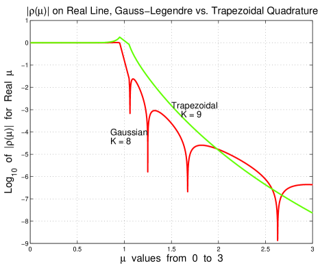
Figure 1: For Hermitian eigenproblems, one only needs a $\rho_{\rm ref}(\mu)$ function that behaves well on the real line, namely, is close to 1 inside $[-1,1]$ and small outside. Because of symmetry, this figure shows $|\rho_{\rm ref}(\mu)|$ only for $\mu\geq 0$. For comparable computational cost of applying $\rho({B}^{-1}A)$ to vectors $U$, Gauss-Legendre performs somewhat better than trapezoidal rule does.

For non-Hermitian problems, $\rho_{\rm ref}(\mu)$ has to “behave well” for $\mu$ in the complex plane. Consequently, for a given quadrature rule, we evaluate $\rho_{\rm ref}(\mu)$ at level curves similar to the boundary $\partial{\cal C}$:

$$\mu(r,t)=r\left[\cos\left(\frac{\pi}{2}(1+t)\right)+{\iota}a\sin\left(\frac{\pi}{2}(1+t)\right)\right].$$

At each $r$ below 1, $0\leq r\leq 1-\delta$ ($\delta$ set to $0.01$), we record the minimum of $|\rho_{\rm ref}|$ over the level curve, and at each $r\geq 1+\delta$, we record the maximum. That is, we examine the function

$$\eta(r)\stackrel{{\scriptstyle\mathrm{def}}}{{=}}\left\{\begin{array}[]{c l}\min_{t}|\rho_{\rm ref}(\mu(r,t))|&\hbox{for $0\leq r\leq 1-\delta$,}\\ \max_{t}|\rho_{\rm ref}(\mu(r,t))|&\hbox{for $1+\delta\leq r$.}\end{array}\right.$$

The function $\eta(r)$ serves as an indicator. An $\eta(r)$ that is close to 1 for $r<1$ and very small for $r>1$ corresponds to an approximate spectral projector that preserves the desired eigenspace well while attenuating the unwanted eigencomponents severely. Figure 2 shows three $\eta(r)$ functions, in logarithmic scale, corresponding to Gauss-Legendre quadrature ($K=8$) on three different shapes of ellipses. Figure 3 shows different $\eta(r)$ functions, in logarithmic scale, corresponding to Gauss-Legendre and trapezoidal rules at different choices of $K$. The domain is set to be a circle. It is interesting to note that while Gauss-Legendre is in general a better choice for Hermitian problems (as Figure 1 suggests), trapezoidal rule seems to fare better for non-Hermitian problems.

We note that the left projector can be approximated in a similar fashion. In particular,

$${B}^{-H}{[\rho({B}^{-1}A)]}^{H}{B}^{H}=Y{[\rho(\Lambda)]}^{H}{X}^{H}{B}^{H}\approx{Y_{\cal C}}{(X_{\cal C})}^{H}{B}^{H}.$$ (8)

Applying this approximate left projector on a $n\times p$ matrix $V$ is

$${B}^{-H}{[\rho({B}^{-1}A)]}^{H}{B}^{H}\,V={\left[\sum_{k=1}^{q}\sigma_{k}(\phi_{k}B-A)\right]}^{-H}\,({B}^{H}\,V).$$ (9)

This involves solving $q$ conjugate-transposed system ${[\sigma_{k}(\phi_{k}B-A)]}^{H}$ each with ${B}^{H}V$ as right-hand-side.

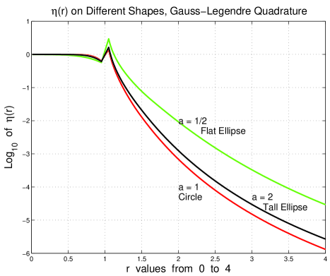
Figure 2: These are the $\eta(r)$ functions corresponding to Gauss-Legendre quadrature with $K=8$ nodes on $[-1,1]$. We exhibit the result for three different elliptical domains. For simplicity, we employ circular domains for the rest of the paper, but different types of domains can be used. See further discussions in Section 6.

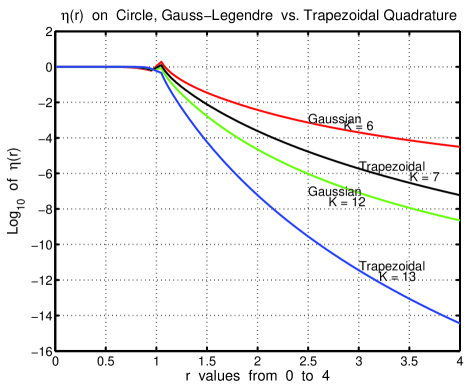
Figure 3: This figure compares Gauss-Legendre quadrature to trapezoidal rule on a circular domain. Because trapezoidal rule uses both $-1$ and $1$ as nodes on the integration interval $[-1,1]$ while Gauss-Legendre uses neither, a $K$-node Gauss-Legendre and a $K+1$-node trapezoidal both require solving $2K$ linear systems when applying the spectral projector $\rho({B}^{-1}A)$ to vectors $U$. The figure suggests that trapezoidal rule works better in general for non-Hermitian problems.

4 Non-Hermitian FEAST

Equation (2) shows that $(\rho(\lambda_{j}),\mathbf{x}_{j})$ is a right eigenpair of $\rho({B}^{-1}A)\mathbf{x}_{j}=\rho(\lambda_{j})B\mathbf{x}_{j}$ for every right eigenpair $(\lambda_{j},\mathbf{x}_{j})$ of $A\mathbf{x}_{j}=\lambda_{j}B\mathbf{x}_{j}$. Moreover ${\rm eig}(\rho(\Lambda_{\cal C}))$ are among the most dominant eigenvalues ${\rm eig}(\rho(\Lambda))$ of the approximate right projector $\rho({B}^{-1}A)$. It is easy to see that corresponding properties hold for the approximate left projector.

Since ${\rm eig}(\rho(\Lambda_{\cal C}))$ are the dominant eigenvalues of $\rho({B}^{-1}A)$, subspace iteration with $\rho({B}^{-1}A)$ is effective in capturing the invariant subspace ${\rm span}(X_{\cal C})$. A Rayleigh-Ritz projection of the original eigenproblem would then allow us to obtain $\Lambda_{\cal C}$ and $X_{\cal C}$. This use of numerical-quadrature-based approximate spectral projector to accelerate subspace iteration followed by Rayleigh-Ritz is the essence of the Hermitian FEAST algorithm [8, 17]. We offer here two generalizations to non-Hermitian problems. The first, Algorithm R-FEAST, uses only one projector; the second, Algorithm Bi-FEAST, uses both.

Algorithm R-FEAST (Right-Projector FEAST)

1:Pick random $\body{U}{0}\in\mathbb{C}^{n\times p}$. Set $k\leftarrow 1$.

2:repeat

3:     $\widehat{U}\leftarrow(\rho({B}^{-1}A)\cdot\body{U}{k-1})$

4:     $\widehat{A}\leftarrow{\widehat{U}}^{H}A\widehat{U},\quad\widehat{B}\leftarrow{\widehat{U}}^{H}B\widehat{U}$.

5:     Solve $\widehat{A}W=\widehat{B}W\widehat{\Lambda}_{(k)}$ for $\widehat{\Lambda}_{(k)}$ and $W$.

6:     $\body{U}{k}\leftarrow\widehat{U}\cdot W$.

7:     $k\leftarrow k+1$

8:until Appropriate stopping criteria

Algorithm Bi-FEAST (Bi-iteration FEAST)

1:Pick random $\body{U}{0}\in\mathbb{C}^{n\times p}$.

2:Get $\body{V}{0}$ where ${(\body{V}{0})}^{H}B\body{U}{0}=I_{p}$. Set $k\leftarrow 1$.

3:repeat

4:     $\widehat{U}\leftarrow(\rho({B}^{-1}A)\cdot\body{U}{k-1}$

5:     $\widehat{V}\leftarrow{B}^{-H}{\rho}^{H}({B}^{-1}A){B}^{H}\cdot\body{V}{k-1}$.

6:     $\widehat{A}\leftarrow{\widehat{V}}^{H}A\widehat{U},\quad\widehat{B}\leftarrow{\widehat{V}}^{H}B\widehat{U}$.

7:     Solve $\widehat{A}=\widehat{B}\,W\,\widehat{\Lambda}_{(k)}\,{Z}^{H}\widehat{B}\;\hbox{for $\widehat{\Lambda}_{(k)},\;W,\;{\rm and}\;Z$}$.

8:     $\body{U}{k}\leftarrow\widehat{U}\cdot W$, $\body{V}{k}\leftarrow\widehat{V}\cdot Z$.

9:     $k\leftarrow k+1$

10:until Appropriate stopping criteria

We state without proofs several key properties of these two algorithms that correspond to generalizations of corresponding theorems in [17]. Number the $\gamma_{j}$s (the eigenvalues of $\rho({B}^{-1}A)$) so that

$$|\gamma_{1}|\geq|\gamma_{2}|\geq\cdots\geq|\gamma_{n}|,$$

and number the eigencomponents of $(A,B)$ accordingly:

$$\gamma_{j}=\rho(\lambda_{j}),\;A\mathbf{x}_{j}=\lambda_{j}B\mathbf{x}_{j},\;{\mathbf{y}}^{H}_{j}A=\lambda_{j}{\mathbf{y}}^{H}_{j}B,\quad j=1,2,\ldots,n.$$

We use the following notations: For integer $\ell$, $1\leq\ell\leq n$,

$$\begin{array}[]{l l}X_{\ell}=[\mathbf{x}_{1},\mathbf{x}_{2},\ldots,\mathbf{x}_{\ell}],&X_{{\ell}^{\prime}}=[\mathbf{x}_{\ell+1},\mathbf{x}_{\ell+2},\ldots,\mathbf{x}_{n}],\\ Y_{\ell}=[\mathbf{y}_{1},\mathbf{y}_{2},\ldots,\mathbf{y}_{\ell}],&Y_{{\ell}^{\prime}}=[\mathbf{y}_{\ell+1},\mathbf{y}_{\ell+2},\ldots,\mathbf{y}_{n}],\\ \Lambda_{\ell}={\rm diag}(\lambda_{1},\lambda_{2},\ldots,\lambda_{\ell}),&\Lambda_{{\ell}^{\prime}}={\rm diag}(\lambda_{\ell+1},\lambda_{\ell+2},\ldots,\lambda_{n}),\\ \Gamma_{\ell}={\rm diag}(\gamma_{1},\gamma_{2},\ldots,\gamma_{\ell}),&\Gamma_{{\ell}^{\prime}}={\rm diag}(\gamma_{\ell+1},\gamma_{\ell+2},\ldots,\gamma_{n}).\end{array}$$

Figures 2 and 3 are illustrative of the general properties of quadrature-based functions $\rho(\mu)$. In general $|\rho(\mu)|\approx 1$ for the $m$ eigenvalues $\lambda\in{\rm eig}(\Lambda_{\cal C})$ of interest. They are among the dominant eigenvalues which include those, if exist, outside of ${\cal C}$ but close to the boundary $\partial{\cal C}$. Thus, there is an integer $m^{\prime}\geq m$, $m^{\prime}\approx m$, such that ${\rm eig}(\Lambda_{\cal C})\subseteq\{\lambda_{1},\lambda_{2},\ldots,\lambda_{m^{\prime}}\}$ and $|\rho(\lambda_{j})/\rho(\lambda_{i})|<1$ for all $i\leq m^{\prime}$, $j>m^{\prime}$. Below are the relevant properties of Algorithms R-FEAST and Bi-FEAST under the assumptions $p\geq m^{\prime}$, $|\gamma_{p+1}/\gamma_{m^{\prime}}|\ll 1$ and other moderate technicalities.

1. There is a constant $\alpha$ such that for each iteration $k$ and $j=1,2,\ldots,p$, elements of the form $\mathbf{x}_{j}+X_{{p}^{\prime}}\mathbf{e}_{j}^{(k)}$ and of the form $\mathbf{y}_{j}+Y_{{p}^{\prime}}\mathbf{f}_{j}^{(k)}$ exist in ${\rm span}(\body{U}{k})$ and ${\rm span}(\body{V}{k})$, respectively, such that $\|{\mathbf{e}_{j}^{(k)}}\|_{2},\|{\mathbf{f}_{j}^{(k)}}\|_{2}\leq\alpha\varepsilon^{k}$ where $\varepsilon=|\gamma_{p+1}/\gamma_{m^{\prime}}|$. In other words, as long as $p$ is chosen big enough so that $|\gamma_{p+1}|$ is small (see Figure 2 for example), as iterations proceed, there are elements in ${\rm span}(\body{U}{k})$ that are close to ${\rm span}(X_{\cal C})$, and elements in ${\rm span}(\body{V}{k})$ that are close to ${\rm span}(Y_{\cal C})$.

2. For Algorithm R-FEAST, as iterations proceed, the eigenvalues of ${\widehat{B}}^{-1}\widehat{A}$ (see Step 4) are the same as those of a matrix of the form

   $$\left[\begin{array}[]{c | c}A^{\prime}_{11}&A^{\prime}_{12}\\ \hline\cr A^{\prime}_{21}&A^{\prime}_{22}\end{array}\right],\quad\hbox{$A^{\prime}_{11}$ is $m^{\prime}\times m^{\prime}$,}$$

   where $\|{A^{\prime}_{11}-\Lambda_{m^{\prime}}}\|_{2}=O(\varepsilon^{k})$, and $\|{A^{\prime}_{21}}\|_{2}=O(\varepsilon^{k})$, $\varepsilon=|\gamma_{p+1}/\gamma_{m^{\prime}}|$. In particular, there are $m^{\prime}$ eigenvalues $\hat{\lambda}_{j}\in{\rm eig}(\body{\widehat{\Lambda}}{k})$, $j=1,2,\ldots,m^{\prime}$, and the corresponding column vectors $\mathbf{u}_{j}^{(k)}$ of $\body{\widehat{U}}{k}$ that satisfy

   $$|\hat{\lambda}_{j}-\lambda_{j}|=O(\varepsilon^{k}),\quad\|{(A-\widehat{\lambda}_{j}B)\mathbf{u}_{j}^{(k)}}\|_{2}=O(\varepsilon^{k}).$$

3. For Algorithm Bi-FEAST, as iterations proceed, the eigenvalues of ${\widehat{B}}^{-1}\widehat{A}$ (see Step 4) are the same as those of a matrix of the form

   $$\left[\begin{array}[]{c | c}A^{\prime}_{11}&A^{\prime}_{12}\\ \hline\cr A^{\prime}_{21}&A^{\prime}_{22}\end{array}\right],\quad\hbox{$A^{\prime}_{11}$ is $m^{\prime}\times m^{\prime}$,}$$

   where $\|{A^{\prime}_{11}-\Lambda_{m^{\prime}}}\|_{2}=O(\varepsilon^{2k})$, and $\|{A^{\prime}_{21}}\|_{2},\|{A^{\prime}_{12}}\|_{2}=O(\varepsilon^{k})$, $\varepsilon=|\gamma_{p+1}/\gamma_{m^{\prime}}|$. In particular, there are $m^{\prime}$ eigenvalues $\hat{\lambda}_{j}\in{\rm eig}(\body{\widehat{\Lambda}}{k})$, $j=1,2,\ldots,m^{\prime}$, and the corresponding column vectors $\mathbf{u}_{j}^{(k)}$ of $\body{\widehat{U}}{k}$, $\mathbf{v}_{j}^{(k)}$ of $\body{\widehat{V}}{k}$ that satisfy $|\hat{\lambda}_{j}-\lambda_{j}|=O(\varepsilon^{2k})$,

   $$\|{(A-\widehat{\lambda}_{j}B)\mathbf{u}_{j}^{(k)}}\|_{2},\quad\|{{(A-\widehat{\lambda}_{j}B)}^{H}\mathbf{v}_{j}^{(k)}}\|_{2}=O(\varepsilon^{k}).$$

   In the absence of ill-conditioning, the discussions of which is omitted here, Bi-FEAST offers faster convergence of eigenvalues (but not the residuals) compared with R-FEAST, albeit at a higher computation cost per iteration – needing to solve the conjugated systems as well. We must mention that R-FEAST is inherently more stable, especially if orthogonalization is applied to $\widehat{U}$ between Steps 4 and 5.

5 Numerical Experiments

Experiments given in Sections 5.1 through 5.4 illustrate the various properties of R-FEAST and Bi-FEAST. They use the matrices QC324 and QC2534 from the NEP collection in [19]. These are standard non-Hermitian eigenvalue problems ($B=I$) that arise in quantum chemistry [20]. These two matrices are similar in properties but differ in size. Figure 4 profiles the location of the eigenvalues in the complex plane. Experiments on QC324 and QC2534 are run in matlab. It turns out that the $m$ eigenvalues in the domain correspond to the most dominant eigenvalues in the approximate projectors, thus $m=m^{\prime}$. Subspace dimensions $p$ in these experiments are chosen moderately bigger than $m$. Section 6 will discuss how $p$ is set in practice. The remaining experiments show FEAST applied to actual scientific applications, run on different computer clusters.

Figure 4: Eigenvalues of the matrix QC2534 from the NEP collection. Eigenvalues distribution of QC234 bears a resemblance.

During the iterations of FEAST, we monitor the $p$ eigenpairs computed from the reduced system (in Step 5 of R-FEAST, for example). A particular (right) eigenpair $(\widehat{\lambda}_{j},\mathbf{u}_{j})$ is considered a candidate if $\widehat{\lambda}_{j}\in{\cal C}$ and $\|{A\mathbf{u}_{j}-\widehat{\lambda}_{j}B\mathbf{u}_{j}}\|_{2}/\|{\mathbf{u}_{j}}\|_{2}$ is reasonably small, typically, $\leq 10^{-4}$. Specifically, we track convergence of

$${\rm Res}_{(k)}\stackrel{{\scriptstyle\mathrm{def}}}{{=}}\max\|{A\mathbf{u}_{j}-\widehat{\lambda}_{j}B\mathbf{u}_{j}}\|_{2}/\|{\mathbf{u}_{j}}\|_{2},\;\;{\rm trace}_{(k)}\stackrel{{\scriptstyle\mathrm{def}}}{{=}}\sum\widehat{\lambda}_{j},$$

over the candidates $\widehat{\lambda}_{j}$s.

5.1 Simple Convergence of R-FEAST

We illustrate the most basic convergence properties with the small (dimension 324) matrix QC324. The domain ${\cal C}$ chosen is the disk of radius $0.01$ centered on the real axis at $-0.5$, containing $m=8$ eigenvalues. We employ Gauss-Legendre quadrature and picked $p=8$. With this choice, $\log_{10}|\rho(\lambda_{p+1})/\rho(\lambda_{m})|=-0.93$. The table here exhibits the expected behavior from both R-FEAST and Bi-FEAST. The eigenvalue and residual convergence rate are linear at roughly $0.9$ digits per iteration, except that eigenvalues in Bi-FEAST converge as fast as $2\times 0.9$ digits per iteration.

$p=m=8$, Gauss-Legendre with $K=8$
	$\log_{10}|\hbox{change in trace}|$		$\log_{10}(\hbox{max of residual})$
Iter.	R-FEAST	Bi-FEAST	R-FEAST	Bi-FEAST
4	-5.4kk	-0.0kk	-5.3kk	-4.8kk
5	-6.4kk	-8.6kk	-6.2kk	-5.7kk
6	-7.3kk	-10.5kk	-7.1kk	-6.6kk
7	-8.2kk	-12.4kk	-8.1kk	-7.6kk
8	-9.2kk	-14.3kk	-9.0kk	-8.5kk
9	-10.2kk	-14.4kk	-9.9kk	-9.4kk
10	-11.1kk	-14.5kk	-10.9kk	-10.3kk
11	-12.1kk	-15.1kk	-11.8kk	-11.3kk
12	-13.1kk	-14.8kk	-12.7kk	-12.2kk
13	-14.1kk	-14.8kk	-13.7kk	-13.1kk
14	-14.7kk	-14.5kk	-14.6kk	-14.1kk

5.2 R-FEAST and Bi-FEAST

This example illustrates the sensitive nature of Bi-FEAST. We have seen in the previous example that Bi-FEAST can offer a faster convergence on the eigenvalues. But as discussed in Section 4, Bi-FEAST is more sensitive to the conditioning of the eigenvalues. This is the case for the matrix QC2534 when the region is chosen to be the disk of radius $0.01$ centered on the real axis at $0.85$, containing 10 eigenvalues. With $p$ set to $p=m+5=15$, Gauss-Legendre quadrature with $K=8$ yields $\log_{10}|\rho(\lambda_{p+1})/\rho(\lambda_{m})|=-2.61$. The condition of the eigenvalues, however, are poor: the products $\|{\mathbf{x}_{j}}\|_{2}\,\|{\mathbf{y}_{j}}\|_{2}$ are of the order of $10^{11}$. The table here shows that indeed the eigenvalues cannot be resolved to be much better than 5 or 6 digits. R-FEAST is able to deliver small residuals, while Bi-FEAST is hampered by the poor conditioning, as it is difficult to maintain bi-orthogonality between the $\mathbf{x}_{j}$ and $\mathbf{y}_{j}$ to full machine precision, precisely because their norms are large.

$p=m+5=15$, Gauss-Legendre with $K=6$
	$\log_{10}|\hbox{change in trace}|$		$\log_{10}(\hbox{max of residual})$
Iter.	R-FEAST	Bi-FEAST	R-FEAST	Bi-FEAST
2	0.6kk	1.0kk	-8.3kk	-4.1kk
3	-0.0kk	-5.3kk	-11.4kk	-5.8kk
4	-5.2kk	-5.3kk	-14.0kk	-5.9kk
5	-6.8kk	-5.4kk	-14.2kk	-6.2kk
6	-6.9kk	-5.3kk	-14.2kk	-5.9kk
7	-7.6kk	-5.3kk	-14.2kk	-6.1kk
8	-6.9kk	-5.6kk	-14.2kk	-6.0kk
9	-6.6kk	-5.4kk	-14.3kk	-6.0kk
10	-6.8kk	-5.7kk	-14.1kk	-5.8kk

5.3 Different Quadratures

Figure 3 in Section 3 suggests that trapezoidal rule may work better in general. This example is consistent with this view, but illustrates some subtlety. Figure 3 depicts minimal convergence rate. Depending on the exact location of the eigenvalues, which is problem specific, a quadrature with a lower minimal convergence rate may actually still converge faster. Here we compute the eigenvalues of QC2534 that reside inside the disk of radius $0.02$, centered on the real line at $-0.17$, which contains 28 eigenvalues. At each of two different settings, the table below exhibits the residual convergence for both Gauss-Legendre and trapezoidal quadrature. The behavior below is consistent with the actual values of $|\rho(\lambda_{p+1})/\rho(\lambda_{m})|$.

R-FEAST, Gauss-Legendre(GL) vs. Trapezoidal(TR)
	$\log_{10}(\hbox{max of residual})$
	$p=m+3=31$		$p=m+6=34$
Iter.	GL-8 nodes	TR-9 nodes	GL-8 nodes	TR-9 nodes
2	-4.1kk	-4.0kk	-4.6kk	-5.7kk
3	-5.6kk	-5.4kk	-6.4kk	-8.2kk
4	-7.0kk	-6.8kk	-8.3kk	-11.3kk
5	-8.7kk	-8.2kk	-10.1kk	-13.8kk
6	-10.9kk	-9.4kk	-11.9kk	-14.2kk
7	-12.9kk	-10.6kk	-13.7kk	-14.3kk
8	-14.1kk	-11.9kk	-14.4kk	-14.4kk

The typical convergence pattern of the residuals is as follows. The subspace dimension $p$ is in general bigger than the number of eigenvalues inside the targeted domain. Some of the residuals that are not targeted (we usually call them collaterals) will converge slowly, or not at all. Figure 5 displays the residuals of our current QC2534 test using Gauss-Legendre with $p$ set to $m+6$. Notice that the 28 targeted residuals converge linearly at the expected rate. Convergence of the collaterals are much slower, and some not at all.

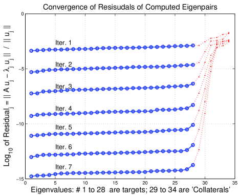
Figure 5: Convergence of residuals: targeted and the “collaterals”. Residuals are sorted to give a more tidy picture.

5.4 General Domain Shapes

FEAST can obviously be applied on general domain shapes as one only need to change the parameterization function $\phi(t)$ in Equation 4 appropriately. Using QC2534 still, we compute the spectrum in three different regions, as shown in Figure 6, using the simple-to-use trapezoidal rule. The table below summarizes the results of running Bi-FEAST.

		Triangle	Square	Semicircle
# eigenvalues	$m$	45	64	9
subspace dim.	$p$	80	100	80
# quadrature nodes	$K$	24	32	16
convergence, measured in digits per iteration
eigenvalues		4	2	5
residuals		2	1	2.5

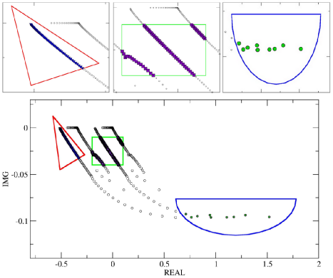
Figure 6: Bi-FEAST is run on three different regions to illustrate that general shapes can be supported easily. The triangle, square, and a semicircle regions are bounded by 3, 4, and 2 segments of curves (or lines) parameterized separately and “glued” together.

5.5 An Electronic Structure Problem

We study the structure of Benzene molecule via a finite element (FEM) discretization of the Kohn-Sham equation. An all-electron potential framework described in [21] is used here. Complex potential interfaces at the edges of the computational domain [22] are then added, resulting in complex symmetric eigenvalue problems. We exhibit here two test cases of quadratic and cubic finite elements, denoted as FEM-Q and FEM-C. The eigenproblems are complex symmetric and in generalized form $Ax=\lambda Bx$. Algorithm Bi-FEAST is run with Gauss-Legendre, $K=12$, on the Phoenix cluster at University of Massachusetts consisting of multiple nodes of Intel^® Xeon^® X5550 2.66GHz processor, 8 cores per node. We use only one target circular domain of radius $3.364\times 10^{-18}$ centered on the real line at $-2.403\times 10^{-17}$. Parallelism on the MPI-process level is exploited by the 24 ($K=12$) linear systems to be solved. When there are enough MPI processes, each linear system can be factored just once for the entire iterative process. This benefit can be seen from the 6-core result of FEM-C below. Within each MPI process, parallelism is utilized by the direct sparse solver Pardiso from Intel^® Math Kernel Library version 10.36. With subspace dimension set to $p=300$, Bi-FEAST converges on the eigenvalues within 4 and 5 iterations, on FEM-Q and FEM-C, respectively. The table presented here emphasizes the ability of Bi-FEAST to utilize the multiple nodes of the system, expressed in “Efficiency.”

	FEM-Q $n=149,192$				FEM-C $n=1,165,485$
	$m=149$, $p=300$				$m=181$, $p=300$
Time
(Ksec)	0.27	0.15	0.10	0.05	1.65	0.86	0.61	0.25
Eff.
(%)	100	92	88	85	100	96	91	110
	1	2	3	6	1	2	3	6
	Number of Nodes, 2 MPI Process/Node

5.6 Quantum Transport

We now seek to obtain the quantum bound-states of a Benzene molecule sandwiched between two electrodes. One can show that an exact derivation of the boundary conditions of the system can give rise to a Hermitian but quadratic (non-linear) eigenvalue problem [23]. From this model, however, one can formulate a more practical linear companion problem but twice larger and non-Hermitian. The determination of the resonant states, that is, solution of this non-Hermitian problem is essential in quantum transport theory [24]. The eigenvalues of interest are located close to the real axis.

A non-Hermitian problem of size $n=98,384$ is solved on a cluster named Endeavor, which is part of the computing infrastructure of Intel Corporation. The search domain is a circle in $\mathbf{k}$-space chosen to contain the energy resonances of the non-linear problem. These resonances correspond to eigenvalues with tiny imaginary parts, in the range $-0.99$eV to $2$eV. Subpsace dimension set to 150, number of quadrature nodes is set to 24, resulting in 48 linear systems in the evaluation of the approximate spectral projector. However, only 24 matrix factorizations are needed because search domain boundary is symmetric with respect to the real axis. In this setting, eigenvalues converge at the second iteration using Bi-FEAST. The following table shows the compute time when Bi-FEAST is run on multiple compute nodes, each node using 16 cores of third generation Intel^® Xeon^® processor.

	Number of compute nodes, 16 cores/node
	1	2	3	4	6	8	12	24
Total time
in seconds	366	154	106	77.0	54.4	44.1	34.8	24.6
Efficiency (%)	100	118	115	118	112	104	90	62

6 Conclusion

In the paper, we have introduced a new non-Hermitian eigensolver with rich inherent parallelism. This paper establishes the theory behind generalizing the FEAST solver for Hermitian problems [8, 17] to non-Hermitian problems in two flavors. Bi-FEAST is the “bullish-but-riskier” sibling of the more conservative R-FEAST. For well-conditioned problems, Bi-FEAST offers faster convergence of eigenvalues; R-FEAST, however, is just as fast in producing small residuals. Both are useful and complement each other. We note here that Bi-FEAST was experimented in [25] by Laux, but without theoretical explanation.

FEAST has a number of signature features. By nature it works equally well regardless whether the targeted spectrum consists of dominant eigenvalues or not. It zooms in on all the targets simultaneously, at practically the same rapid convergence rate. The dimension of the subspaces, as well as the linear systems that need to be solved remained unchanged throughout a fixed targeted domain ${\cal C}$. Although the linear systems are of the form $\phi_{k}B-A$, they are not shifts in the familiar sense. The $\phi_{k}$s are not meant to be close to any eigenvalues but merely correspond to nodes of a numerical quadrature rule. Under ideal situations, they are not near any eigenvalues and none of the linear systems is ill-conditioned. Every one of these features is distinct from those associated with popular non-Hermitian eigensolvers such as unsymmetric Lanczos [26], Arnoldi [11], or Jacobi-Davidson [27, 28]. FEAST is fundamentally based on subspace iteration, whereas [18, 29], despite their use of quadrature techniques, are more related to Krylov methods. The quadratures there are used to approximate higher-order matrix moments. In contrast, the quadratures used in FEAST are used to approximate the zeroth moments, which correspond to spectral projectors.

The FEAST algorithms require the user to set a subspace dimension $p$, which should exceed $m$, the number of eigenvalues in ${\cal C}$. In practice, $p$ is often chosen based on a priori knowledge or experience, or trial-and-error. A more elaborate theory exists, similar to those detailed in [17] for the Hermitian case, on estimation of the $m$. For example, one can use the eigenvalues of ${\widehat{V}}^{H}B\widehat{U}$ ($\widehat{U},\widehat{V}$ from Steps 4 and 5 of Bi-FEAST) to estimate the eigenvalue count $m$.

Opportunities for further work present themselves naturally, in the directions of approximation theory, matrix analysis and parallel computing. At FEAST’s core is a rational function close to 1 inside a domain ${\cal C}$, and 0 outside. Here we have used either a Gauss or trapezoidal quadrature rule to construct this rational function. In general, possibility abounds for other quadrature rules, either general or domain, ${\cal C}$, specific (see [30] for example). Alternatively, one can view this as a function approximation problem. Chebyshev polynomials [31, 32] which work well on the real line (for Hermitian problems) would not work on the complex plane in terms of approximating the $\pi(\mu)$ function in Equation (5): Polynomials are analytic and must obey the maximum modulus theorem (see [33] for example). Rational approximation can contribute fruitfully here. We have already seen one such case for Hermitian problem where Zolotarev approximation is shown to outperform Gauss quadrature [34].

In non-Hermitian matrix computations, it is customary to focus on the class of diagonalizable matrices. How well a quadrature-based approximate spectral projector handles a general Jordan block, and what the resulting implication on FEAST’s convergence behavior in the face of deficient eigenvectors will be, are worthy pursuit that requires classical matrix and perturbation analysis.

Last but not least, FEAST offers multiple levels of parallelism: multiple target domains, multiple linear systems, with multiple right hand sides. Exploiting these parallelism fully, automatically, require much work still. On the highest level, fast partitioning of a region in the complex plane to subregions, each containing roughly the same number of eigenvalues, for the obvious sake of load balancing, is nontrivial. Challenging software engineering work is required to automatically distribute and coordinate the linear solvers – direct or iterative, sparse or dense – on multiple right hand sides, among multiple nodes, cores and threads.

References

- [1] Y. Saad, “Chebyshev acceleration techniques for solving nonsymmetric eigenvalue problems,” Mathematics of Computation, vol. 42, no. 166, pp. 567–588, 1984.
- [2] Y. Saad, Numerical Methods for Large Eigenvalue Problems. Philadelphia: SIAM, 2011.
- [3] S. Odermatt, M. Luisier, and B. Witzigmann, “Bandstructure calculation using the method for arbitrary potentials,” Journal of Applied Physics, vol. 97, no. 4, pp. 046104–046104–3, 2009.
- [4] D. Bindel and S. Govindjee, “Elastic PMLs for resonator anchor loss,” Internationl Journal for Numerical Methods in Engineering, vol. 64, pp. 789–818, 2005.
- [5] F. Tisseur and K. Meerbergen, “The quadratic eigenvalue problem,” SIAM Review, vol. 43, pp. 235–286, 2001.
- [6] E. Anderson, Z. Bai, C. Bischof, S. Blackford, J. Demmel, J. Dongarra, A. Greenbaum, S. Hammarling, A. McKenney, and D. Sorenson, LAPACK Users Guide. Philadelphia: SIAM, 3 ed., 1999.
- [7] J. Demmel, Applied Numerical Linear Algebra. Philadelphia: SIAM, 1997.
- [8] E. Polizzi, “Density-matrix-based algorithm for solving eigenvalue problems,” Physical Review B, vol. 79, no. 115112, 2009.
- [9] Z. Bai, J. Demmel, A. Ruhe, and H. van der Vorst, Templates for the Solution of Algebraic Eigenvalue Problems. Philadelphia: SIAM, 2000.
- [10] J. Cullum and R. A. Willoughby, Lanczos Algorithms for Large Symmetric Eigenvalue Computations. Boston: Birkhäuser, 1985.
- [11] R. Lehoucq and D. Sorensen, “Deflation techniques for an implicitly restarted Arnoldi iteration,” SIAM Journal on Matrix Analysis and Applications, vol. 17, pp. 789–821, 1996.
- [12] B. Parlett, The Symmetric Eigenvalue Problem. Philadelphia: SIAM, 1998.
- [13] A. Sameh and Z. Tong, “The trace minimization method for the symmetric generalized eigenvalue problem,” Journal on Computational and Applied Mathematics, vol. 123, pp. 155–175, 2000.
- [14] A. H. Sameh and J. A. Wisniewski, “A trace minimization algorithm for the generalized eigenvalue problem,” SIAM Journal on Numerical Analysis, vol. 19, no. 6, pp. 1243–1259, 1982.
- [15] A. Bai, J. Demmel, J. Dongarra, A. Petitet, H. Robinson, and K. Stanley, “The spectral decomposition of nonsymmetric matrices on distributed memory parallel computers,” SIAM Journal on Scientific Computing, vol. 18, pp. 1446–1461, September 1997.
- [16] Z. Bai and J. Demmel, “Using the matrix sign function to compute invariant subspaces,” SIAM Journal on Matrix Analysis and Applications, vol. 19, pp. 205–225, January 1998.
-
[17]
P. T. P. Tang and E. Polizzi, “FEAST as subspace iteration accelerated by
approximate spectral projection.”
arXiv:1302.0432 [math.NA], submitted for publication, 2013. - [18] T. Sakurai and H. Sugiura, “A projection method for generalized eigenvalue problems using numerical integration,” Journal on Computational and Applied Mathematics, vol. 159, pp. 119–128, 2003.
- [19] Z. Bai, D. Day, J. Demmel, and J. Dongarra, “Test matrix collection (non-Hermitian eigenvalue problems),” tech. rep., University of Kentucky, September 1996.
- [20] S. I. Chu, “Complex quasivibrational energy formalism for intense-field multi photon and above-threshold dissociation: Complex-scaling Fourier-grid Hamiltonian method,” Journal of Chemical Physics, vol. 94, pp. 7901–7909, 1991.
- [21] A. Levin, D. Zhang, and E. Polizzi, “FEAST fundamental framework for electronic structure calculations: Reformulation and solution of the muffin-tin problem,” Computer Physics Communications, vol. 183, pp. 2370–2375, 2012.
- [22] L. Lehtovaara, V. Havu, and M. Puska, “All-electron time-dependent density functional theory with finite elements: Time-propagation approach,” Journal of Chemical Physics, vol. 135, no. 154104, 2012.
- [23] Z. Shao, W. Porod, C. S. Lent, and D. J. Kirkner, “An eigenvalue method for open-boundary quantum transmission problems,” Journal of Applied Physics, vol. 78, pp. 2177–2186, 1995.
- [24] E. Polizzi, N. Abdallah, O. Vanbésien, and D. Lippens, “Space lateral transfer and negative differential conductance regimes in quantum waveguide junctions,” Journal of Applied Physics, vol. 87, pp. 8700–8706, 2000.
- [25] S. E. Laux, “Solving complex band structure problems with the FEAST eigenvalue algorithm,” Physical Review B, vol. 86, no. 075103, 2012.
- [26] B. N. Parlett, D. R. Taylor, and Z. A. Liu, “A look-ahead Lanczos algorithm for unsymmetric matrices,” Mathematics of Computation, vol. 44, pp. 105–124, 1985.
- [27] P. Arbenz and M. E. Hochstenbach, “A Jacobi-Davidson method for solving complex symmetric eigenvalue problems,” SIAM Journal on Scientific Computing, vol. 25, no. 5, pp. 1655–1673, 2004.
- [28] G. L. G. Sleijpen and H. A. V. D. Vorst, “A Jacobi-Davidson iteration method for linear eigenvalue problems,” SIAM Review, vol. 42, no. 2, pp. 267–293, 2000.
- [29] T. Ikegami, T. Sakurai, and U. Nagashima, “A filter diagonalization for generalized eigenvalue problems based on sakurai-sugiura projection method,” Journal on Computational and Applied Mathematics, vol. 233, pp. 1927–1936, 2010.
- [30] D. Bailey and J. Borwein, “Hand-to-hand combat with thousand-digit integrals,” Journal of Computational Science, vol. 3, pp. 77–86, 2012.
- [31] Y. Zhou and Y. Saad, “A Chebyshev-Davidson algorithm for large symmetric eigenproblems,” SIAM Journal on Matrix Analysis and Applications, vol. 29, no. 3, pp. 954–971, 2007.
- [32] Y. Zhou, Y. Saad, M. L. Tiago, and J. R. Chelikowsky, “Self-consistent-field calculations using Chebyshev-filtered subspace iteration,” Journal of Computational Physics, vol. 219, pp. 172–184, 2006.
- [33] G. Polya and G. Latta, Complex Variables. New York: John Wiley and Sons, Inc., 1974.
- [34] G. Viaud, “The FEAST algorithm for generalised eigenvalue problems,” Master’s thesis, University of Oxford, Oxford, England, 2012.