Numerical Study of the Two-Species Vlasov-Ampère System: Energy-Conserving Schemes and the Current-Driven Ion-Acoustic Instability
Abstract
In this paper, we propose energy-conserving Eulerian solvers for the two-species Vlasov-Ampère (VA) system and apply the methods to simulate current-driven ion-acoustic instability. The algorithm is generalized from our previous work for the single-species VA system [9] and Vlasov-Maxwell (VM) system [8]. The main feature of the schemes is their ability to preserve the total particle number and total energy on the fully discrete level regardless of mesh size. Those are desired properties of numerical schemes especially for long time simulations with under-resolved mesh. The conservation is realized by explicit and implicit energy-conserving temporal discretizations, and the discontinuous Galerkin (DG) spatial discretizations. We benchmarked our algorithms on a test example to check the one-species limit, and the current-driven ion-acoustic instability. To simulate the current-driven ion-acoustic instability, a slight modification for the implicit method is necessary to fully decouple the split equations. This is achieved by a Gauss-Seidel type iteration technique. Numerical results verified the conservation and performance of our methods.
Keywords: Two-species Vlasov-Ampère system, energy conservation, discontinuous Galerkin methods, current-driven ion-acoustic waves, anomalous resistivity.
1 Introduction
In this paper, we propose energy-conserving Eulerian solvers for the two-species Vlasov-Ampère (VA) system and apply the methods to simulate current-driven ion-acoustic instability. The two-species VA model describes the evolution of the distribution functions for a single species of electrons and ions under the influence of the self-consistent electric field. Accurate numerical simulation for this system is crucial for the understanding of ion-acoustic waves, ion-acoustic turbulence in fusion plasmas and magnetic reconnection in space plasmas.
In the literature, a class of well-established methods for the Vlasov equation is the particle-in-cell (PIC) methods [3, 25]. In PIC methods, the macro-particles are advanced in a Lagrangian framework, while the field equations are solved on a mesh. The main advantage of the PIC method is its relatively low cost for high dimensional problems, but it suffers from statistical noise built intrinsically in those methods. Our approach in this paper is to use a grid-based Vlasov solver, which does not have statistical noise and can resolve the low-density regions more accurately. While there are abundant literature on grid-based Vlasov solver for single-species VA or Vlasov-Poisson (VP) system, e.g. [7, 34, 4, 23, 26, 15, 21], there are relatively fewer published works for the two-species system. In [19, 20, 18], Fourier transformed methods are used to compute two-species VP system for electron and ion holes. In [28], the hydrodynamic and quasi-neutral limits of the two-species VP system are studied by the finite difference WENO method. In [33, 32], the MacCormack method is employed for calculation of anomalous resistivity and the nonlinear evolution of ion-acoustic instability. A detailed study of the comparison of the MacCormack method and a PIC method for anomalous resisitivity in current-driven ion-acoustic waves can be found in [35].
One of the main focus of this paper is to develop fully discrete energy-conserving methods. The total energy is a nonlinear quantity that depends on the distribution functions of both species as well as the electric field. To achieve energy conservation, special care must be taken to design both the temporal and spatial discretizations. In this work, we generalize our previous methods for the single-species VA system [9] and Vlasov-Maxwell (VM) system [8] to the two-species system. The main feature of our method is that it can preserve the total energy on the fully discrete level regardless of mesh size. This is advantageous for long time simulation, guaranteeing no generation of annulation of spurious energy, and avoiding artifacts such as plasma self heating or cooling [14]. Previously, several PIC methods have been proposed to conserve the total energy for the single-species VA system [6] and the VM system [30]. Finite difference and DG methods [22, 2] were proposed to conserve the total energy of VP systems on the semi-discrete level. Our method is the first Eulerian solver to achieve conservation of total energy and particle number simultaneously for the two-species system. This is done by using the newly developed energy-conserving temporal discretizations [9, 8], and the discontinuous Galerkin (DG) spatial discretizations [12]. In fact, the approach in this paper can be easily adapted to multi-species VA or VM systems as well.
For the two-species system, one of the other computational challenges besides conservation is the multiscale nature of the problem. Because ions are much heavier than electrons, electrons move faster and the temporal scale for electrons is smaller than that of the ions. For efficient calculations, hybrid and multiscale particle codes have been developed [5, 29]. We mention in particular the implicit particle methods [17, 13] and electron sub-cycling techniques [1]. In this paper, we aim at resolving the physical phenomena that happen at the electron time scale. Therefore the typical time step satisfies , where is the electron plasma frequency. In the velocity space, we take the common approach of choosing different computational domain for the velocity space of the electrons and ions, and taking larger grids in electrons than ions. This is allowed because the two species are only coupled together through the electric field. We want to remark that in some applications, it would be natural to follow the slower ion time scales. In those scenarios, the electron equation becomes stiff and a multiscale temporal solver would be necessary. However, we do not attempt to address this issue in the current paper and leave it to our future work.
The rest of this paper is organized as follows: in Section 2, we describe the equations under consideration. In Section 3, we develop our energy-conserving schemes and discuss their properties. The additional term involving the spatial average of the current density will cause the split equation to be globally coupled. To resolve this issue, a Gauss-Seidel iteration is employed. Section 4 is devoted to numerical results, including the test of one-species limit and the simulations of the current-driven ion-acoustic waves (CDIAW), in which we perform numerical tests on an ensemble of 100 VA simulations with random phase perturbations to investigate the anomalous resistivity with a reduced mass ratio. Finally, we conclude with a few remarks in Section 5.
2 The Two-Species VA System
In this section, we describe the two-species VA system and its dimensionless version. The two-species VA system for electrons and ions is given by
| (2.1a) | |||
| (2.1b) | |||
where ; for electrons and for ions. is the physical domain. is the probability distribution function of the particle species . denotes the particle mass of species . is the magnitude of the electron charge. In (2.1b),
is the total current density of the two species. is the external current that may be generated by the gradients of an external magnetic field .
Given that density, time and space variables are in units of the background electron number density , the electron plasma period and the electron Debye radius , respectively, the distribution function is scaled by , where is the electron thermal speed, is the electron temperature; the electric field and the current density are scaled by and , respectively. Keeping the same notations and for the rescaled unknowns and variables, (2.1) becomes the dimensionless two-species VA system
| (2.2a) | |||
| (2.2b) | |||
where , i.e. , . with .
The two-species VA system (2.2) conserves many physical quantities, such as the total particle number for each species , the entropy and any integral of functions of , as well as the total energy
if . This is true when no external current is present, i.e. , as well as for the CDIAW discussed in Section 4.2. In CDIAW, the external current is a constant chosen to balance the internal current such that [32], where denotes the spatially averaged electric field. In (2.2), this is equivalent to letting , where denotes the spatially averaged current for . With , we will get , therefore , and the energy conservation is implied. For simplicity, in the rest of the paper, we only consider the situation of or , with . In particular, we adopt the following notation
| (2.3a) | |||
| (2.3b) | |||
to incorporate the discussion of both cases, where the inclusion of is for the CDIAW simulations with .
3 Numerical Methods
In this section, we develop energy-conserving numerical methods for the two-species VA system (2.3). Our methods are generalized from the energy-conserving methods introduced in [9, 8] for one-species VA and VM systems. By proper design, the methods in this paper can achieve similar conservation properties as those in [9, 8], and can be readily adapted to multi-species VA systems.
3.1 Temporal discretizations
In [9, 11], second and higher order temporal discretizations are introduced for the one-species systems. The unique features are that those methods are designed to preserve the discrete total energy. For simplicity, in this paper, we will only consider two types of second-order time stepping methods for the two-species system: one being the fully explicit method, and the other one being the fully implicit method with operator splitting.
The explicit method is given as follows
| (3.4a) | |||
| (3.4b) | |||
| (3.4c) | |||
and the term in (3.4b) is for the case of . Similar to [9], we denote the scheme above to be Scheme-1, namely, this means .
The fully implicit method is based on the energy-conserving operator splitting for (2.3) as follows:
Both the split equations maintain the same energy conservation as the original system,
In particular,
where in the last equality we have used the assumption , therefore in the case of .
Now we will solve each of the subequations by the second-order implicit midpoint method. In particular, we denote the implicit midpoint method for system (a),
| (3.5a) | |||
| (3.5b) | |||
as . Similarly, for Equation (b), the implicit midpoint method
| (3.6a) | |||
| (3.6b) | |||
is denoted as . Note that here we have abused the notation, and use superscript , to denote the sub steps in computing equations (a), (b) rather than the whole time step to compute the VA system. Finally, we define
Through simple Taylor expansions, we can verify that both schemes are second order accurate in time, also they satisfy discrete energy conservation as illustrated in the theorem below.
Theorem 3.1
With periodic boundary conditions in domain, the schemes above preserve the discrete total energy , where
in Scheme-1 and Scheme-2 for both the case of and , with .
Proof. When , the proof is similar to [9] and is omitted.
In the case of , with , in Scheme-1, we derive
Therefore, , if .
From (3.4), the additional contribution of term to the total energy difference at compared to is
Therefore, we established total energy conservation for Scheme-1 in this case. The proof for Scheme-2 is similar and omitted.
3.2 Fully discrete methods
In this section, we will discuss the spatial discretizations and formulate the fully discrete schemes. In particular, we consider two approaches: one being the explicit scheme, the other being the split implicit scheme. Here, we follow our previous work [9, 8] and use discontinuous Galerkin (DG) methods to discretize the variable. The DG methods are shown to have excellent conservation properties, and when applied to one-species VA and VM systems, the methods can be designed to achieve fully discrete energy conservation [9, 8]. For the two-species system, the main difference in our schemes compared to [9] is the inclusion of the additional species, and the inclusion of term. This causes some additional difficulties as outlined in Section 3.2.3.
3.2.1 Preliminaries
When discretizing the velocity space, it is necessary to truncate the domain into a finite computational region. This is a reasonable assumption as long as the computational domain is taken large enough so that the probability distribution functions vanish at the boundary. For the two-species system, due to the intrinsic scale difference between ions and electrons, we shall use different regions for the two species. In particular, we denote , to be the truncated velocity domain for electrons and ions. While the typical size of , since the ion speed is generally slower, the size of would be smaller and . As for the domain, without loss of generality, periodic boundary condition is assumed. We remark here that our methods can be easily adapted to other types of boundary conditions.
Now we are ready to introduce the mesh and underlying piecewise polynomial spaces. We define and be partitions of and , respectively, with and being Cartesian elements or simplices. Notice that we use the same mesh in domain for the two species due to their coupling in the Ampère equation. However, the mesh in domain is different for the two-species due to the size difference between and .
The meshes for the two species are defined as . Let be the set of the edges of and be the set of the edges of ; then the edges of will be , . Here we take into account the periodic boundary condition in the -direction when defining and .
We will make use of the following discrete spaces: for ,
| (3.7a) | ||||
| (3.7b) | ||||
| (3.7c) | ||||
and
| (3.8a) | ||||
| (3.8b) | ||||
where is the number of dimension for the domain, denotes the set of polynomials of total degree at most on . The discussion about those spaces for Vlasov equations can be found in [11, 10].
For piecewise functions defined with respect to or , we further introduce the jumps and averages as follows. For any edge , with as the outward unit normal to , , and , the jumps across are defined as
and the averages are
where . are used to denote or .
3.2.2 The explicit method
In this subsection, we will describe the explicit DG methods formulated with time diescretization Scheme-1. In particular, we look for , , such that for any ,
| (3.9a) | |||
| (3.9b) | |||
| (3.9c) | |||
Here and are outward unit normals of and , respectively. Following the discussion in [9], to deal with filamentation, we use the dissipative upwind numerical fluxes, i.e.,
| (3.10a) | ||||
| (3.10b) | ||||
The upwind fluxes in (3.9c) are defined similarly.
3.2.3 The implicit method
In this subsection, we would like to design fully discrete implicit DG methods with Scheme-2. The key idea is to solve each split equation in their respective reduced dimensions. A complete discussion of similar methods for one-species models on general mesh has been included in [9]. In this paper, the main difficulty for applying such an approach is for the case of , which causes a coupling in the direction for equation (b).
For simplicity, below we will describe the scheme in detail under 1D1V setting. For one-dimensional problems, we use a mesh that is a tensor product of grids in the and directions, and the domain is partitioned as follows:
where is chosen large enough as the cut-off speed for species . The mesh is defined as
Let , be the length of each interval. be the Gauss quadrature points on and be the Gauss quadrature points on . Now we are ready to describe our scheme.
Algorithm Scheme-a
To solve from to
- 1.
-
2.
Let be the unique polynomial in , such that .
Algorithm Scheme-b
Case 1: . This case is similar to the discussion of [9].
To solve from to
- 1.
-
2.
Let be the unique polynomial in , such that . Let be the unique polynomial in , such that .
To solve (3.12), a Jacobian-free Newton-Krylov solver [27] (KINSOL) is necessary. Notice we need to set a tolerance parameter in KINSOL, and that may cause some slight deviation in the conservation.
Case 2: with . This case is different due to the coupling from term. To solve from to
a direct generalization of (3.12) would cause a nonlinearly coupled system in the whole space because involves all elements in . To resolve this issue, we employ a simple Gauss-Seidel iteration as outlined below.
-
1.
Initialize with , .
-
2.
Iterate on , solve
(3.13a) (3.13b) until convergence, i.e. , where is a preset tolerance parameter.
-
3.
Set , .
We notice that the (3.13a) can be implemented explicitly, i.e. for ,
where and This would determine uniquely .
The linear systems resulting from (3.13b) can be evaluated at each Gauss quadrature nodes in direction, i.e. for each species , , we seek and , such that
| (3.14) |
holds for any test function , where the flux terms in (3.14) are chosen as the upwind flux, similar to Section 3.2.2. Then we let be the unique polynomial in , such that .
Finally, we recall and this completes the description of the fully implicit method.
3.2.4 Properties of the fully discrete methods
In this subsection, we summarize the conservation properties of the fully discrete methods for the two-species VA system. The proof of the theorems below is similar to [9] by utilizing Theorem 3.1 and the properties of Gauss quadrature formulas, and thus is omitted.
Theorem 3.2 (Total particle number conservation)
Theorem 3.3 (Total energy conservation)
Theorem 3.4 ( stability)
The fully implicit DG scheme described in Section 3.2.3 is stable, i.e.
We notice that the theorems above do not take into account the deviation of from zero at and the tolerance parameters in the implicit solves. Those factors are the only possible error sources in the numerical computations for particle number and energy conservation.
4 Numerical Results
In this section, we demonstrate the performance of our methods in the 1D1V setting. For simplicity, we use uniform meshes in and directions, while we note that nonuniform mesh can also be used under the DG framework. We use quadratic polynomial spaces and test Scheme-1 with space , and Scheme-2 with space , respectively.
The time step is chosen according to
Notice that the explicit scheme has to satisfy the CFL restriction for stability, while the implicit method can allow large CFL numbers in the computation.
Two numerical examples are considered in this section: a two-species model with which has the limit of Landau damping when the mass ratio , and the CDIAW with and .
For Scheme-2, we use KINSOL from SUNDIALS [24] to solve the nonlinear algebraic systems (3.12) and (3.13b) resulting from the discretization of equation (b), and we set the tolerance number to be . The tolerance is set to be in the Gauss-Seidel iteration solving the system (3.13).
4.1 Testing the one-species limit
In this subsection, we consider the two-species VA system with a fixed temperature ratio and varying mass ratio to test the one-species limit of our methods. In particular, by letting the initial condition be
| (4.15a) | ||||
| (4.15b) | ||||
where and , we will recover the one-species Landau damping in the limit of . This initial condition corresponds to ions in a uniform equilibrium state with a slightly perturbed electron distribution.
The computational domain for is set to be , with . The domain of velocity for electron and ion is chosen to be with and with , respectively, such that on the boundaries. We use a mesh of uniform cells in the direction, and cells in the direction. Our numerical examples are performed with two sets of mass ratios, (the reduced mass ratio) and (the real mass ratio). The real mass ratio corresponds to heavy ions that are essentially immobile.
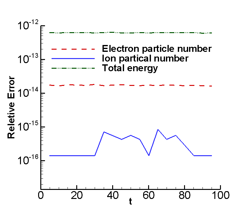
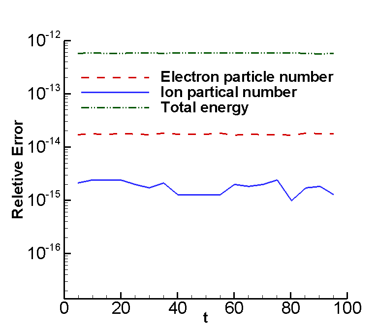
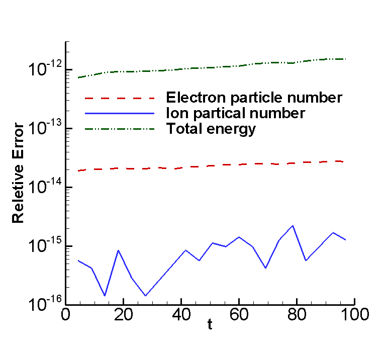
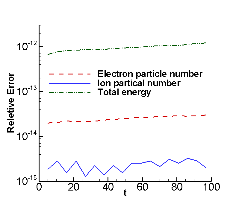
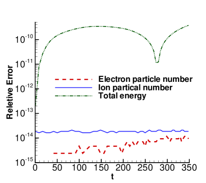
We first verify the conservation of total particle number and total energy for our schemes. Figure 4.1 shows the absolute value of relative error of the total particle number and total energy for Scheme-1 ( typical time step size ) and Scheme-2 ( typical time step size ) with two sets of mass ratios with and . We can see that all errors stay small, below for the whole duration of the simulation. In Figure 4.2, we use a coarse mesh (, , ) to plot the errors in the conserved quantities to demonstrate that the conservation properties of our schemes are mesh independent. We use Scheme-2 to demonstrate the behavior. Upon comparison with the results from finer mesh in Figures 4.1, we conclude that the mesh size has no impact on the conservation of total particle number and total energy as predicted by Theorems 3.2 and 3.3. This verify the conservation properties are independent of mesh sizes, and we are allowed to use even under-resolved mesh to achieve high accuracy in particle number and energy conservations.
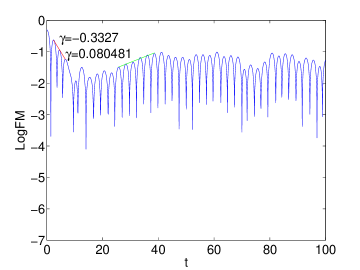
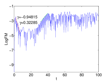
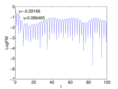
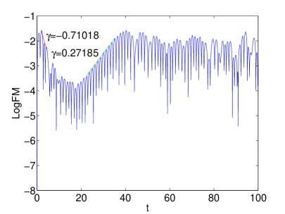
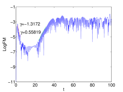
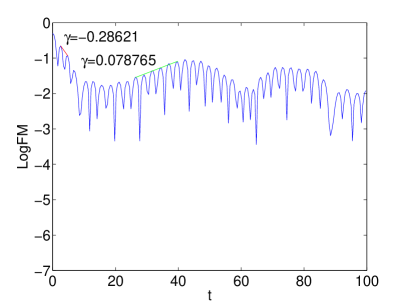
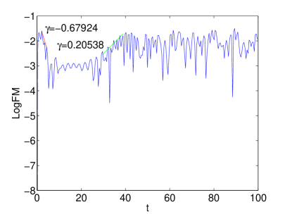
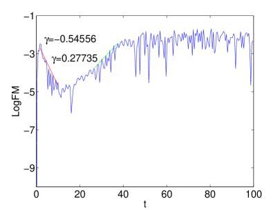
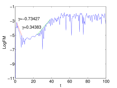
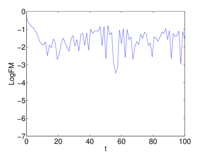
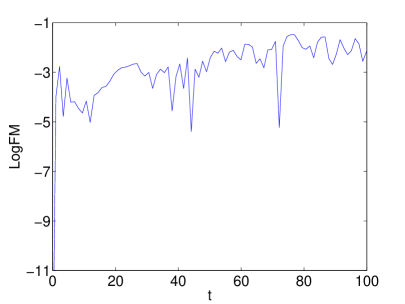
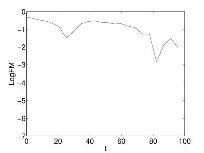
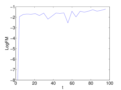
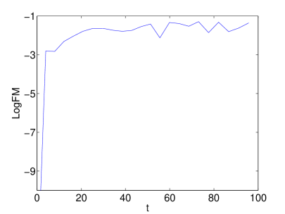
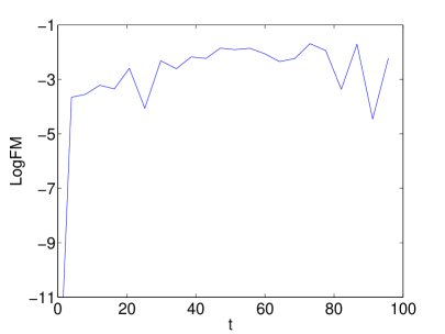
Next, we compare the difference of numerical simulations between different mass ratios. We plot the first four Log Fourier modes for the electric field. The -th Log Fourier mode for the electric field is defined as
They are crucial quantities to investigate the qualitative behavior of the solution [7]. By comparing Figures 4.3 and 4.4, we see that both mass ratios demonstrate similar qualitative behavior for the four modes. Upon a detailed comparison to the one-species Landau damping result [9], the real mass ratio clearly yields decay and growth rates that are much closer to the one-species Landau damping, showing the convergence of the model to the one-species limit when .
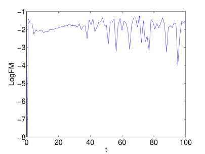
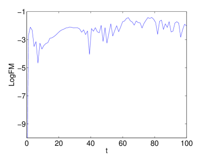
Finally, we investigate the influence of the time step size on the behavior of the solutions. In Figures 4.4, 4.5, 4.6 and 4.7, we plot the results using the real mass ratio with varying CFL numbers by the implicit scheme. Although the four simulations are all numerically stable, we clearly observe that the numerical runs with (i.e. in the unscaled variables) in Figures 4.6 and 4.7 fail to capture the subtle electron kinetic effects. Naturally, larger time steps will filter out high frequency in time, and if the electron kinetic effects are important, it would be necessary to use time step size smaller than .


4.2 Current-driven ion-acoustic instability
In this subsection, we perform a detailed numerical study of the current-driven ion-acoustic instability. Ion-acoustic waves are natural wave modes in unmagnetized plasmas. Current-driven ion-acoustic instability are generated by giving the electrons an initial uniform drift velocity relative to the ions such that where is the threshold for the ion-acoustic instability. This test example corresponds to the case of the two-species VA system with , .
The initial conditions of the distribution functions are given by
| (4.16a) | ||||
| (4.16b) | ||||
where is the number of modes permitted in the simulation, is a random phase, is the thermal fluctuation level, is the uniform drift velocity for the electrons and . The initial condition for the electric field
is obtained by the Poisson equation and clearly satisfies .
In the numerical runs, we use simulation parameters as listed in Table 4.1, which are the rescaled version of the parameters used in Table 1 of [32]. In particular, we focus on the reduced mass ratio with instead of the real mass ratio. As demonstrated in [32], the reduced mass ratio yields qualitatively similar results as the real mass ratio, but enables faster computations. This is because the real mass ratio would require a large number of electron velocity grid points in order to accommodate the relatively small range of resonant phase velocities. By using the reduced mass ratio, the run time of the simulation is kept to a reasonable level for us to perform 100 simulations with random phase perturbations.
In Table 4.1, are the smallest and largest wavelengths of linearly unstable ion-acoustic wave modes calculated by solving numerically the linear dispersion relation. The domain for is set to be , where . Let denotes the wave number. for with . The domain of velocity for electron and ion is chosen to be and , respectively, such that on the boundaries. are the smallest and largest phase velocity of the unstable wave modes calculated from the solution to the linear dispersion. The resolution of the velocity grids is controlled by the phase velocities of the growing wave modes, such that there are three velocity points in the linear unstable region () so that interaction with the unstable wave modes is possible [32]. Under this scaling, in (4.16a). Under our scaling, all the variables ploted in the figures of the following sections can be read as the values of quantities of the reference [32] after multiplied by the corresponding factor listed in the last column of Table 4.1.
Parameters S_1(reduced mass ratio) Variables plotted Scaled factor m_i/m_e 25 t ω_pe T_e/T_i 2 x 3.97 λ_min 7.98 θ_e^m 2 λ_max 426.60 f_e 11.81 v_ph,min 0.23 f_i 11.81 v_ph,max 0.29 η 7.58×10^5 V_c,e 10.30 E 0.504 V_c,i 2.87 κ 0.252 N_x 500 N_v,e, N_v,e 890
Our first test in this subsection is to verify the conservation properties of the proposed methods Scheme-1 and Scheme-2. In the numerical simulations, we use (typical time step size ) for Scheme-1 and (typical time step size ) for Scheme-2. Figure 4.8 shows the absolute value of the relative error of the total particle number and total energy for Scheme-1 and Scheme-2 with simulations parameters . We observe that the relative errors stay small, below for Scheme-1 and below for Scheme-2. The errors of total energy for Scheme-2 are slightly larger mainly due to the error in the Gauss-Seidel iteration relating to the preset tolerance parameter .

One of the important quantity to consider is the anomalous resistivity defined as [16]
| (4.17) |
The resistivity in our simulations is scaled by and calculated at each time step using a first order backward finite difference method for the time derivative. More discussions about the calculation of resistivity can be found in [35].
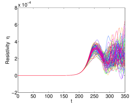
We first perform a numerical test with . This drift velocity is not large enough to trigger instability [35] and the wave eventually got damped as illustrated in Figure 4.9(a). In the rest of the paper, we focus on the case of , which is a drift velocity chosen large enough to result in the ion-acoustic instability. Similar to [32], to study the impact of the initial random phases , we perform an ensemble of 100 simulations with random using the explicit method Scheme-1. For each of the 100 simulations, the phases of the initial white noise were randomly picked out of the uniform distribution on .
Figure 4.9(b) shows the time evolution of anomalous resistivity for three representative simulations Run No. 1, 8, 98. All the simulation runs of ion-acoustic waves show similar resistivity evolution, while the exact values of the anomalous resistivity differ from one simulation to the another, due to the initial fluctuations in the random phases. As in [32], we also mark different periods of the evolution of the resistivity using four regimes. This can be explained by comparing with Figure 4.10(a) where the fastest-growing mode of Run No. 1 is plotted.
- •
-
•
: the linear regime. The anomalous resistivity remains close to zero and the only growing modes in the system are the linear modes. During this time period, the fastest-growing mode grows exponentially in time as predicted by the linear theory.
-
•
: the quasi-linear regime. The resistivity rises rapidly for to a peak at and the fastest-growing mode starts deviating from exponential growth and saturates.
-
•
: the nonlinear regime. The resistivity is relatively stable, oscillating about the resistivity level reached at the end of the quasi-linear regime.
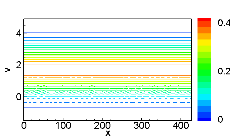
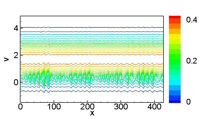
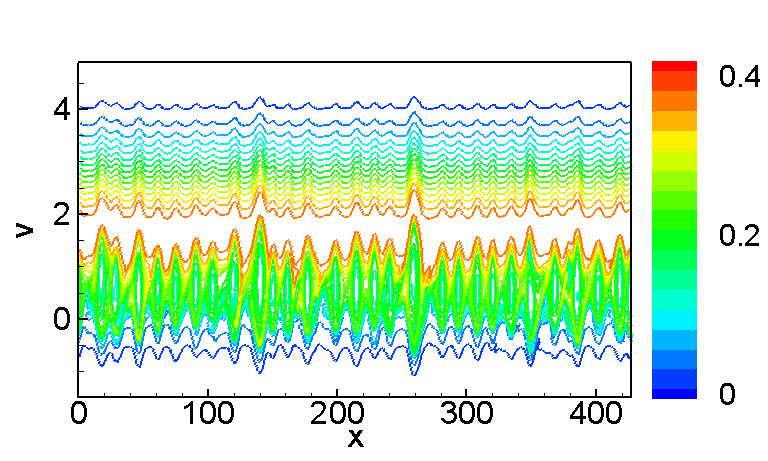
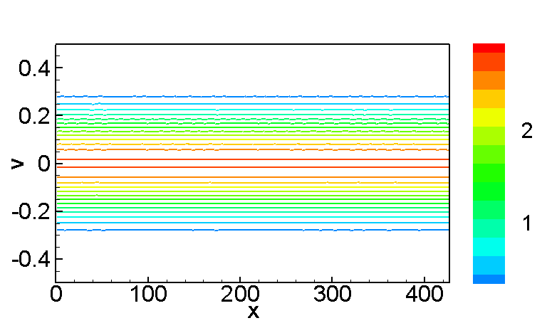
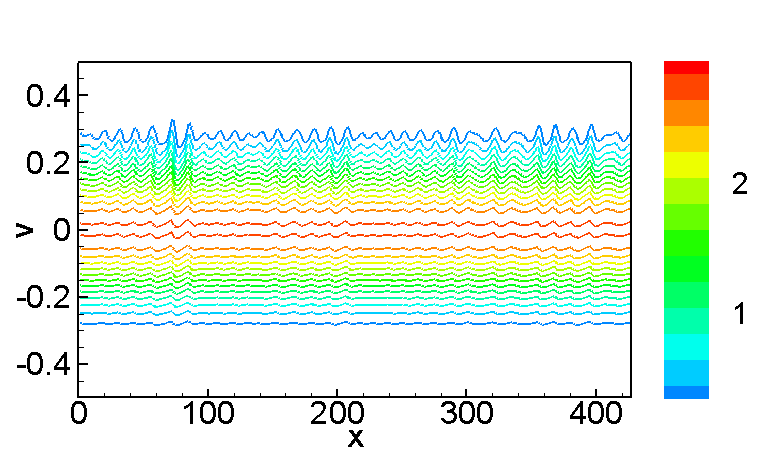
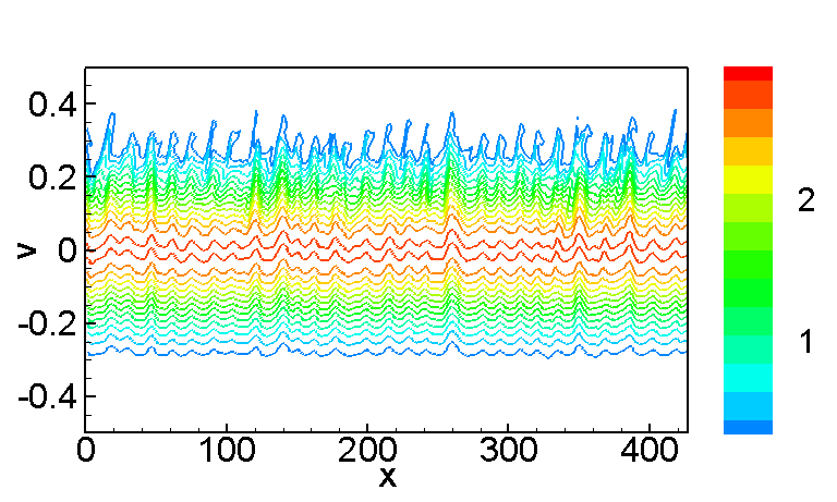
In Figure 4.10(b), we plot the spatially averaged distributions functions of ions and electrons at selected time for Run No 1. We zoom in velocity space and in order to see the details. The two distributions are shown at the beginning to the simulation (), near quasi-linear saturation , and which is during the nonlinear regime. We obtain qualitatively similar results to [32]. Namely, the development of the plateau formation for the distributions functions since the quasi-linear regime indicates the momentum exchange between electrons and ions via the ion-acoustic waves. In Figure 4.11 and 4.12, we plot the probability distribution functions of electron and ion at for Run No. 1. We have zoomed in velocity space in order to see the detail structure of the solutions. At (a time frame in the linear regime ), the electron and ion distributions still stay rather close to the initial distributions. At (a time frame in the quasi-linear regime), deviations from the initial configurations are visible. In particular for the electron distributions, small trapping regions start to form. This is more prominent at (a time frame in the nonlinear regime) and several large trapping islands are displayed in the electron distribution functions. Such observations are consistent with the depiction in Figure 4.10(b).
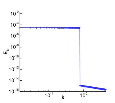
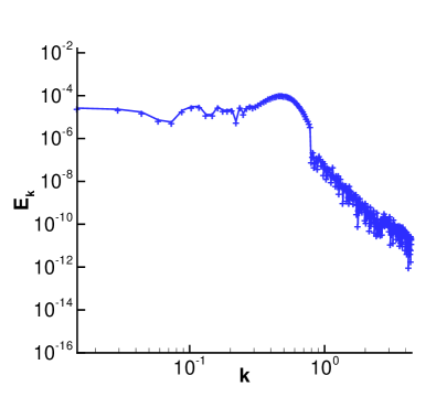
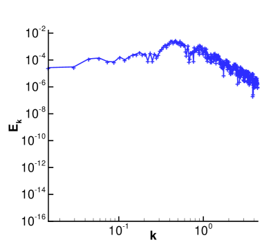
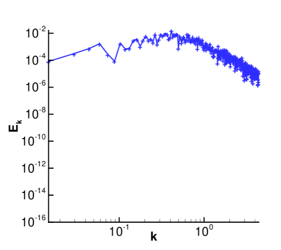
To further show the details of the solutions at those given times, we plot the electric spectrum in -space in Figure 4.13. At t=0, we show the electric field spectrum associated with the initial condition, notice for , the nonzero values are due to the double precision accuracy used in the numerical simulations. For all later times, the spectrum demonstrate similar results as in [32]. At time , the wave power is above the initial noise field. Since the quasilinear regime, we can observe that the wave energy cascades into wave modes outside the linear resonant region, and generally all modes have increased in power. The development of the power law electric field spectrum is evidence of nonlinear wave-wave coupling.
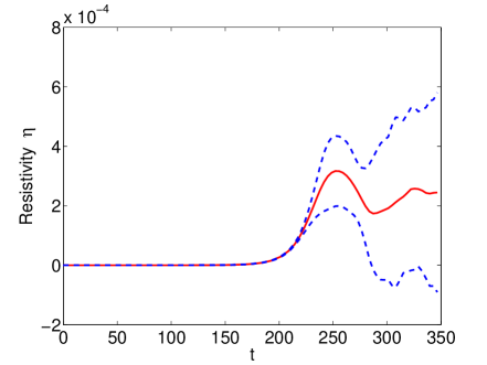
To verify the impact of the initial random phase field, next we perform statistical study of the 100 VA simulations similar to [32]. We notice that due to the CFL conditions of Scheme-1, each simulation has slightly different time step sizes. To benchmark the meaningful quantitative statistical analysis with [32], we interpolate all the simulations with piecewise cubic Hermite interpolation. The time step and resistivity values discussed in the following context are the values after interpolation. The overall conclusion is similar to [32]. Figure 4.14 over plot the time evolution of all 100 anomalous resistivities, which proves the similarity and diversity in the behavior of the resistivity. In Figure 4.14, we plot the mean value of the resistivity calculated by averaging the value of the 100 resistivity values at each time step, and the three standard deviations from the mean. Comparing 4.14 and 4.14, we see that the range of resistivity values is well confined in of the mean, as would be expected by a Gaussian distribution.
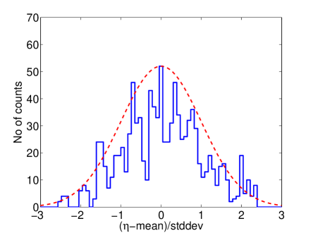
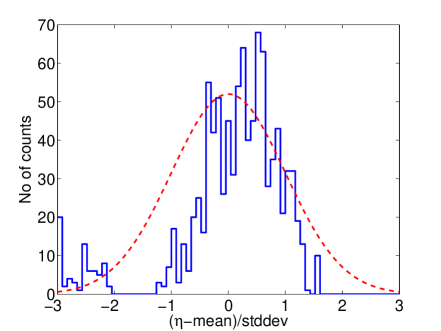
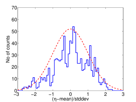
To investigate this further, we plot histograms of the probability distribution of the standardized resistivity values in Figure 4.15 for three time periods from three different regimes in the evolution of the instability to study how well they fit into the Gaussians. The standardized value of at is , where is the ensemble mean value of at , and is the standard deviation of at . Each histogram comprises of all the standardized resistivity values from 10 consecutive time steps. Figure 4.15(a) shows the probability distribution of the standardized resistivity values for during the linear regime of the instability. The distribution appears to fit a Gaussian reasonably well. Figure 4.15(b) shows the probability distribution of the standardized resistivity values for during the quasi-linear regime of the instability. The distribution is sharply peaked and with a left tail longer than the right, which seems deviate from a Gaussian. Figure 4.15(c) shows the probability distribution of the standardized resistivity values for during the nonlinear regime of the instability. The distribution appears to be symmetric and approximately Gaussian.
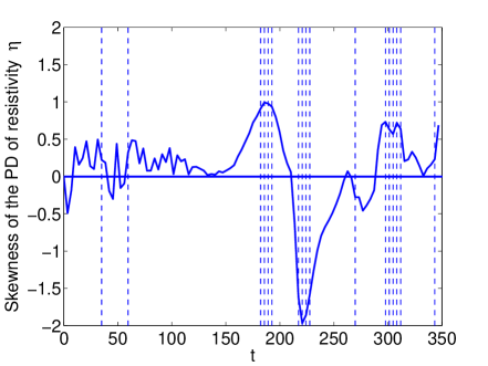
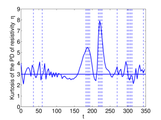
As in [32], we perform a chi-square test for the standardized resistivity values at each time step, where we tested the goodness of fit to a Gaussian distribution of mean zero and unit standard deviation of each one of the probability distributions of standardized resistivity values at the 0.05 and 0.01 significance level. Overall, the test fails in 16.8% of the time steps at the 0.05 level and at 7.1% at the 0.01 level, (compared to 8.4% and 1.8% in [32]) which suggests that the distributions of resistivity values may not fit a Gaussian at all times. Figure 4.16 shows the times when chi-square test fails at the 0.05 level (dashed lines). Figure 4.16 also shows the time evolution of the skewness and kurturtosis of the resistivity distributions. The skewness of the resistivity distributions remains close to 0 for most of the time evolution, implying that the distributions are mostly symmetrical. The kurtosis of the distributions remains close to 3 for most to the time evolution, consistent with a Gaussian. We also observe that the amplitude of the oscillations in the values of skewness and kurtosis increases as we approach quasi-linear saturation and beyond. This deviation from the expected Gaussian values can also be seen in Figure 4.15(b): the skewness is negative, which indicates that the left tail is longer; the kurtosis is well above three indicating a more sharply peaked distribution than a Gaussian. Although the exact values of skewness and Kurtosis are different from [32], the overall shape and the qualitative behavior remains the same. We remark that our plots seem smoother in time because of the Hermite interpolation we used when post-processing the data.
5 Concluding Remarks
In this paper, we develop explicit and implicit energy-conserving Eulerian solvers for the two-species VA system and apply the methods to simulate current-driven ion-acoustic instability. The overall results show excellent conservation of the total particle number and total energy regardless of the mesh size as predicted by the theoretical studies. The implicit methods, though do not suffer from CFL restrictions, still require to fully resolve the electron kinetic effects. For the current-driven ion-acoustic instability, we perform an ensemble of 100 VA simulations with random phase perturbations to investigate the anomalous resistivity with a reduced mass ratio. The results agree well with previous studies. In future work, it would be interesting to generalize such schemes to simulate multi-species systems when the electron kinetic effects are of less importance. A multiscale algorithm would be desired to follow the ion dynamics and to be able to take time step sizes with .
Acknowledgments
YC is supported by grants NSF DMS-1217563, DMS-1318186, AFOSR FA9550-12-1-0343 and the startup fund from Michigan State University. AJC is supported by AFOSR grants FA9550-11-1-0281, FA9550-12-1-0343 and FA9550-12-1-0455, NSF grant DMS-1115709 and MSU foundation SPG grant RG100059. We gratefully acknowledge the support from Michigan Center for Industrial and Applied Mathematics.
References
- [1] J. Adam and A. Gourdin Serveniere. Electron sub-cycling in particle simulation of plasma. Journal of Computational Physics, 47(2):229–244, 1982.
- [2] B. Ayuso and S. Hajian. High order and energy preserving discontinuous Galerkin methods for the Vlasov-Poisson system. 2012. preprint.
- [3] C. K. Birdsall and A. B. Langdon. Plasma physics via computer simulation. Institute of Physics Publishing, 1991.
- [4] J. P. Boris and D. L. Book. Flux-corrected transport. III. minimal-error FCT algorithms. Journal of Computational Physics, 20:397–431, 1976.
- [5] J. U. Brackbill and B. I. Cohen. Multiple time scales. In Multiple time scales.. JU Brackbill, BI Cohen (Editors). Computational Techniques, Vol. 3. Academic Press, Inc., volume 1, 1985.
- [6] G. Chen, L. Chacón, and D. Barnes. An energy-and charge-conserving, implicit, electrostatic particle-in-cell algorithm. Journal of Computational Physics, 230(18):7018–7036, 2011.
- [7] C. Z. Cheng and G. Knorr. The integration of the Vlasov equation in configuration space. J. Comput. Phys., 22(3):330–351, 1976.
- [8] Y. Cheng, A. J. Christlieb, and X. Zhong. Energy conserving schemes for Vlasov-Maxwell systems. Submitted.
- [9] Y. Cheng, A. J. Christlieb, and X. Zhong. Energy conserving schemes for Vlasov-Ampère systems. Journal of Computational Physics, 256:630–655, 2014.
- [10] Y. Cheng, I. M. Gamba, F. Li, and P. J. Morrison. Discontinuous Galerkin methods for Vlasov-Maxwell equations. 2013. submitted.
- [11] Y. Cheng, I. M. Gamba, and P. J. Morrison. Study of conservation and recurrence of Runge–Kutta discontinuous Galerkin schemes for Vlasov-Poisson systems. J. Sci. Comput., 56:319–349, 2013.
- [12] B. Cockburn and C.-W. Shu. Runge-Kutta discontinuous Galerkin methods for convection-dominated problems. J. Sci. Comput., 16:173–261, 2001.
- [13] B. I. Cohen, A. B. Langdon, and A. Friedman. Implicit time integration for plasma simulation. Journal of Computational Physics, 46(1):15–38, 1982.
- [14] B. I. Cohen, A. B. Langdon, D. W. Hewett, and R. Procassini. Performance and optimization of direct implicit particle simulation. J. Comput. Phys., 81(1):151–168, 1989.
- [15] N. Crouseilles and T. Respaud. A charge preserving scheme for the numerical resolution of the Vlasov-Ampere equations. Commun. Comput. Phys., 10:1001–1026, 2011.
- [16] R. C. Davidson and N. T. Gladd. Anomalous transport properties associated with the lower-hybrid-drift instability. Physics of Fluids, 18(10):1327–1335, 1975.
- [17] J. Denavit. Time-filtering particle simulations with . Journal of Computational Physics, 42(2):337–366, 1981.
- [18] B. Eliasson. Numerical simulations of the fourier-transformed vlasov-maxwell system in higher dimensionstheory and applications. Transport Theory and Statistical Physics, 39(5-7):387–465, 2010.
- [19] B. Eliasson and P. Shukla. Dynamics of electron holes in an electron–oxygen-ion plasma. Physical review letters, 93(4):045001, 2004.
- [20] B. Eliasson and P. Shukla. Production of nonisothermal electrons and langmuir waves because of colliding ion holes and trapping of plasmons in an ion hole. Physical review letters, 92(9):095006, 2004.
- [21] N. Elkina and J. Büchner. A new conservative unsplit method for the solution of the Vlasov equation. J. Comput. Phys., 213(2):862–875, 2006.
- [22] F. Filbet and E. Sonnendrücker. Comparison of Eulerian Vlasov solvers. Computer Physics Communications, 150:247–266, 2003.
- [23] F. Filbet, E. Sonnendrücker, and P. Bertrand. Conservative numerical schemes for the Vlasov equation. J. Comp. Phys., 172:166–187, 2001.
- [24] A. C. Hindmarsh, P. N. Brown, K. E. Grant, S. L. Lee, R. Serban, D. E. Shumaker, and C. S. Woodward. Sundials: Suite of nonlinear and differential/algebraic equation solvers. ACM T. Math. Software, 31(3):363–396, 2005.
- [25] R. W. Hockney and J. W. Eastwood. Computer simulation using particles. McGraw-Hill, New York, 1981.
- [26] R. B. Horne and M. P. Freeman. A new code for electrostatic simulation by numerical integration of the vlasov and ampere equations using maccormack’s method. Journal of Computational Physics, 171(1):182 – 200, 2001.
- [27] D. A. Knoll and D. E. Keyes. Jacobian-free Newton-Krylov methods: a survey of approaches and applications. J. Comput. Phys, 193(2):357–397, 2004.
- [28] S. Labrunie, J. A. Carrillo, and P. Bertrand. Numerical study on hydrodynamic and quasi-neutral approximations for collisionless two-species plasmas. Journal of Computational Physics, 200(1):267–298, 2004.
- [29] A. S. Lipatov. The hybrid multiscale simulation technology: an introduction with application to astrophysical and laboratory plasmas. Springer, 2002.
- [30] S. Markidis and G. Lapenta. The energy conserving particle-in-cell method. J. Comput. Phys., 230(18):7037 – 7052, 2011.
- [31] A. W. T. Nicholas A. Krall. Principles of plasma physics. McGraw-Hill, New York, 1973.
- [32] P. Petkaki, M. P. Freeman, T. Kirk, C. E. J. Watt, and R. B. Horne. Anomalous resistivity and the nonlinear evolution of the ion-acoustic instability. Journal of Geophysical Research, 111(A01205), 2006.
- [33] P. Petkaki, C. E. J. Watt, R. B. Horne, and M. P. Freeman. Anomalous resistivity in non-Maxwellian plasmas. Journal of Geophysical Research: Space Physics, 108(A12), 2003.
- [34] E. Sonnendrücker, J. Roche, P. Bertrand, and A. Ghizzo. The semi-Lagrangian method for the numerical resolution of the Vlasov equation. J. Comp. Phys., 149(2):201–220, 1999.
- [35] C. E. J. Watt. Wave-particle interactions and anomalous resistivity in collisionless space plasmas. PhD thesis, Univ. of Cambridge, 2001.