Effects of interactions on the dynamics of driven cold atoms

Abstract

The quantum fidelity was introduced by Peres to study some fingerprints of classically chaotic behavior in the quantum dynamics of the corresponding systems. In the present paper the signatures of classical dynamics near elliptic points and of interactions between particles are characterized for kicked systems. In particular, the period of the fidelity resulting of the interactions is found using analytical and numerical calculations. A mechanism leading to the oscillations with the intermediate period is proposed. It is of a semiclassical origin and results of the interplay between the oscillations of the width of the wave packets and the rotation of their center around the elliptic fixed point.

I Introduction

Effects of inter-particle interactions on the dynamics of driven systems were the subject of several recent works Quantum_accelerator ; Transition_to_instability ; Wave_packet_dynamics ; Mark_paper . In the present paper these studies will be extended to the exploration of the effects of interactions on the quantum fidelity.

The concept of quantum fidelity was introduced by Peres Peres_fidelity as a fingerprint of classical chaos in quantum dynamics. It has subsequently been extensively utilized in theoretical Jalabert_Pastawski_Y19 ; Decay_Loschmidt_Y20 ; Sensitivity_Chaotic_Systems_Y34 ; Saturation_of_Fidelity_Y35 and experimental studies Saturation_of_Fidelity_Y35 ; Decay_of_QM_correlations_Y38 ; Hyperfine_spectroscopy_Y37 ; Revivals_of_coherence_Y36 (for a review see Review_Y21 ). In absence of interactions the quantum fidelity, in a mixed system (in some parts of phase space the dynamics is chaotic and in other parts regular) was studied Yevgeny_paper . In particular, it was found that the fidelity exhibits oscillations in time, and their periods are found to be related to the periods of the motion in regular parts of phase space Yevgeny_paper .

In the present work we will study the effects of the inter-particle interactions on the periods of the fidelity. The fidelity is defined by

$$F\left(t\right)=|\left\langle\psi_{1}|\psi_{2}\right\rangle|^{2}$$ (1)

where

$$\left|\psi_{1}\left(t\right)\right\rangle=e^{i\frac{H_{1}t}{\hbar}}\left|\phi_{0}\right\rangle$$ (2)

and

$$\left|\psi_{2}\left(t\right)\right\rangle=e^{i\frac{H_{2}t}{\hbar}}\left|\phi_{0}\right\rangle$$ (3)

are propagated by the Hamiltonians $H_{1}$ and $H_{2}$, that are of the same form but with different values of the parameters and $\left|\phi_{0}\right\rangle$ is the initial state.

We note that the fidelity $F\left(t\right)$ is related to the integral over Wigner functions,

$$F\left(t\right)=\intop_{-\infty}^{\infty}\intop_{-\infty}^{\infty}dxdpW_{1}\left(x,p\right)W_{2}\left(x,p\right)$$ (4)

where $W_{1}$ and $W_{2}$ are the Wigner functions of $\left|\psi_{1}\right\rangle$ and $\left|\psi_{2}\right\rangle$ ,respectively.

The general form of the Wigner function is

$$W\left(x,p\right)=\frac{1}{\pi\cdot\hbar}\intop_{-\infty}^{\infty}d\xi\cdot\psi^{*}\left(x+\xi\right)\psi\left(x-\xi\right)e^{\frac{2ip\xi}{\hbar}}.$$ (5)

Without interactions, the specific system we will study is defined by the Hamiltonian Yevgeny_paper

$$H=\frac{p^{2}}{2}-Ke^{-\frac{x^{2}}{2}}\sum_{n=-\infty}^{\infty}\delta\left(t-n\right)$$ (6)

where

$$p=-i\tau\partial_{x}$$ (7)

and

$$\tau=\frac{\hbar T}{m\Delta^{2}}$$ (8)

is the rescaled $\hbar$ ,satisfying

$$\left[x,p\right]=i\tau$$ (9)

The Hamiltonian is in dimensionless units. In physical units $T$ is the time between the kicks, $\triangle$ is the width of the pulses of the kicking potential, while $m$ is the mass of the particles.

The one step evolution operator is

$$U=e^{-i\frac{p^{2}}{2\tau}}\exp\left(i\frac{K}{\tau}e^{-\frac{x^{2}}{2}}\right).$$ (10)

The corresponding classical map is

$$p_{n+1}=p_{n}-Kx_{n}e^{-\frac{x_{n}^{2}}{2}}$$ (11)

$$x_{n+1}=x_{n}+p_{n+1}.$$ (12)

Its phase portrait is shown in Fig. 1.

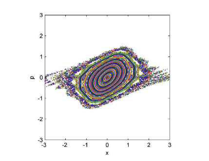
Figure 1: (Color online) The phase portrait for $K=1$. Colors distinguish different orbits.

In previous explorations Mark_Update the interaction term was introduced only between the kicks and the $\frac{p^{2}}{2}$ term was replaced by

$$H_{I}=\frac{p^{2}}{2}+\beta\left|\psi\left(x\right)\right|^{2}$$ (13)

where $\beta$ is the strength of the interactions. Therefore, between the kicks the dynamics are modeled by the nonlinear Schrödinger equation (NLSE), known also as the Gross Pitaevskii equation (GPE),

$$i\tau\frac{\partial\psi}{\partial t}=H_{I}\psi.$$ (14)

In the expression for the evolution operator $e^{-\frac{p^{2}}{2\tau}}$ should be replaced by another evolution operator. In the calculation of the fidelity Mark_Update , the frequencies that were found in the absence of interactions were observed. In addition, a different new frequency was found. Unlike the other frequencies, this frequency is not related in any simple way to the frequencies of the underlying classical system. It was found to depend on the strength inter-particle interactions and can be considered as a signature of the interactions in the fidelity.

The main problem with introducing the interaction term between kicks Mark_Update is that it requires the numerical solution of the NLSE in each interval between kicks. This process is highly time consuming since it requires the solution of a differential equation between the kicks, and it is impossible to propagate the system for very long times.

For this reason, in the current work we study a model that is defined by the evolution operator

$$U=e^{-i\frac{p^{2}}{2\tau}}\exp\left(\frac{i}{\tau}\text{$\left(Ke^{-\frac{x^{2}}{2}}+\beta\left|\psi\left(x\right)\right|^{2}\right)$}\right)$$ (15)

where the interactions are introduced at the kicks. The Hamiltonian of this model is

$$H=\frac{p^{2}}{2}-Ke^{-\frac{x^{2}}{2}}\sum_{n=-\infty}^{\infty}\delta\left(t-n\right)+\beta\left|\psi\left(x\right)\right|^{2}\sum_{n=-\infty}^{\infty}\delta\left(t-n\right).$$ (16)

This model is related to one studied by Shepelyansky Shepelyansky_93 .

It should be clarified that the purpose of this study is purely theoretical, with the aim to shed light on the fingerprints of interparticle interactions in the fidelity. We will focus our studies on the fidelity for wavepackets started near the central elliptic fixed point.

In Section II we will introduce a harmonic oscillator model describing the motion near the fixed point and discuss the modifications required. In Section III we will introduce an approximate theory for the fidelity oscillations and in Sections IV and V we will confront it with numerical results. The results are summarized and discussed in Section LABEL:sec:summary-and-conclusions.

II A model for the motion near the central elliptic point

Near the fixed point $\left(x,p\right)=\left(0,0\right)$, the dynamics are approximately determined by the tangent map of the fixed point. For this purpose we linearize the classical map (11), (12) around the fixed point $x=p=0$. This gives the equation for the deviations from this point

$$\left(\begin{array}[]{c}\delta x_{n+1}\\ \delta p_{n+1}\end{array}\right)=\left(\begin{array}[]{cc}\left(1-K\right)&1\\ -K&1\end{array}\right)\left(\begin{array}[]{c}\delta x_{n}\\ \delta p_{n}\end{array}\right).$$ (17)

The eigenvalues of this map are

$$\alpha_{\pm}=\frac{\left(2-K\right)}{2}\pm\frac{\sqrt{K\left(4-K\right)}}{2}\equiv e^{\pm i\omega}$$ (18)

with

$$\omega=\arctan\left(\frac{\sqrt{K\left(4-K\right)}}{2-K}\right),$$ (19)

which is the angular velocity of the points around the origin. In the vicinity of the fixed point, the system behaves like a harmonic oscillator with a frequency $\omega$. Classically, the motion of the trajectories, starting near the elliptic fixed point, $x=p=0$, stays there because the region is bounded by KAM curves that surround this point. We consider here two Hamiltonians $H_{1}$ and $H_{2}$ that differ only by the values of the stochasticity parameter $K$, taking the values $K_{1}=1$ and $K_{2}=1.01$.

For $K=K_{1}=1$, one finds

$$\omega_{1}=1.047$$ (20)

and for $K=K_{2}=1.01$,

$$\omega_{2}=1.053.$$ (21)

The parameters were chosen so that the map has a pronounced central island as shown in Fig. 1. The qualititative behavior should be similar for all $0<K<4$ (see Yevgeny_paper ).

The periods of the regular trajectories deviate from the ones found at the elliptic point by (19). The deviation increases with the deviation from the elliptic point. This is similar to the situation when a small anharmonicity is added to the harmonic potential. Therefore, for wave packets initiated not exactly at the elliptic point, one has to add an anharmonic term to model the dynamics. The result is that the different parts of the packet are exposed to different frequencies. Therefore, an initially prepared Gaussian wave packet spreads in phase space. This was indeed verified for Gaussian wave packets in a harmonic well with a small anharmonic correction Echoes . As the wave packet propagates, revivals are found for a very long time. Fortunately, in presence of interactions, localization of Gaussian wave packets is possible, as was found for an anharmonic well with inter-particle interactions modeled by the Gross Pitaevskii equation (GPE) Mark_paper (see also Wave_packet_dynamics ). Interactions and nonlinearity may balance each other to preserve the Gaussian wave packet Mark_paper .

In the following section, the dynamics of particles in a harmonic well with a small anharmonic perturbation will be studied analytically, for weak inter-particle interactions. Following the discussion in the present section, it will be assumed that in the vicinity of this elliptic point the motion can be described by a Gaussian wave packet.

III Fidelity for weak interactions

In this section an estimate for the oscillations of the fidelity for a wavepacket that is initially a coherent state of a harmonic oscillator defined by the Hamiltonian

$$H=\frac{p^{2}}{2m}+\frac{1}{2}m\omega^{2}x^{2}.$$ (22)

III.1 The Wigner function of a coherent state

A coherent state for the harmonic oscillator defined by the Hamiltonian (22) is coherent_comp

$$\psi_{0}=\left(\frac{m\omega}{\pi\hbar}\right)^{\frac{1}{4}}\exp\left(\frac{i}{\hbar}p_{0}\left(t\right)-\frac{m\omega}{2\hbar}\left(x-x_{0}\left(t\right)\right)^{2}\right)e^{-\frac{i}{2\hbar}x_{0}\cdot p_{0}}e^{-i\frac{\omega t}{2}}$$ (23)

where $x_{0}\left(t\right)$and $p_{0}\left(t\right)$ denote the classical trajectory in phase space. The state (23) is an eigenstate of the annihilation operator and satisfies the time dependent Schrödinger’s equation

$$i\hbar\frac{\partial\psi_{0}}{\partial t}=-\frac{\hbar^{2}}{2m}\frac{\partial^{2}\psi_{0}}{\partial x^{2}}+\frac{1}{2}m\omega^{2}x^{2}\psi_{0}$$ (24)

The Wigner function of this coherent state is found from the definition (5):

$$W_{0}\left(x,p\right)=\frac{1}{\pi\cdot\hbar}e^{-\frac{m\omega}{\hbar}\left(x-x_{0}\right)^{2}}e^{-\frac{\left(p-p_{0}\right)^{2}}{m\omega\hbar}}$$ (25)

III.2 The fidelity for coherent states in absence of interactions

Let $\omega_{1}$ and $\omega_{2}$ be the frequencies of two harmonic oscillators, whose potentials differ slightly. The Wigner functions for these wavefunctions are $\left(i=1,2\right)$

$$W_{i}\left(x,p\right)=\frac{1}{2\pi\sigma_{x_{i}}\sigma_{p_{i}}}\exp\left(-\frac{1}{2}\left(\frac{\left(x-x_{i}\left(t\right)\right)^{2}}{\sigma_{x_{i}}^{2}}+\frac{\left(p-p_{i}\left(t\right)\right)^{2}}{\sigma_{p_{i}}^{2}}\right)\right)$$ (26)

where

$$\sigma_{x_{i}}^{2}=\frac{\hbar}{2m\omega_{i}}$$ (27)

and

$$\sigma_{p_{i}}^{2}=\frac{m\omega_{i}\hbar}{2}$$ (28)

The fidelity in absence of interactions is calculated using (4) and is given by

$$F=Ce^{-\frac{1}{2}\left(s_{x}+s_{p}\right)}$$ (29)

where the parameters are given by

$$C=\frac{2}{\pi\hbar^{2}}\sqrt{\frac{\sigma_{x_{1}}^{2}\sigma_{x_{2}}^{2}\sigma_{p_{1}}^{2}\sigma_{p_{2}}^{2}}{\left(\sigma_{x_{1}}^{2}+\sigma_{x_{2}}^{2}\right)\left(\sigma_{p_{1}}^{2}+\sigma_{p_{2}}^{2}\right)}}$$ (30)

$$s_{x}=\frac{\left(x_{1}\left(t\right)-x_{2}\left(t\right)\right)^{2}}{\sigma_{x_{1}}^{2}+\sigma_{x_{2}}^{2}}$$ (31)

$$s_{p}=\frac{\left(p_{1}\left(t\right)-p_{2}\left(t\right)\right)^{2}}{\sigma_{p_{1}}^{2}+\sigma_{p_{2}}^{2}}$$ (32)

The classical trajectories are given by

$$\left(x_{1},p_{1}\right)=\rho\left(\cos\left(\omega_{1}t\right),-m\omega_{1}\sin\left(\omega_{1}t\right)\right)$$ (33)

and

$$\left(x_{2},p_{2}\right)=\rho\left(\cos\left(\omega_{2}t\right),-m\omega_{2}\sin\left(\omega_{2}t\right)\right)$$ (34)

where

$$\rho=x_{1}\left(0\right)=x_{2}\left(0\right)$$ (35)

Therefore, (31) can be written in the form

$$s_{x}=\frac{\rho^{2}}{\sigma_{x_{1}}^{2}+\sigma_{x_{2}}^{2}}\left(1+\frac{1}{2}\left(\cos\left(2\omega_{1}t\right)+\cos\left(2\omega_{2}t\right)\right)-\cos\left(\delta\omega\cdot t\right)-\cos\left(\omega_{s}t\right)\right)$$ (36)

where

$$\omega_{s}=\omega_{1}+\omega_{2}$$ (37)

and

$$\delta\omega=\omega_{1}-\omega_{2}$$ (38)

Similarly,

$$s_{p} = \frac{\rho^{2}m^{2}}{\sigma_{p_{1}}^{2}+\sigma_{p_{2}}^{2}}\left(\frac{\omega_{1}^{2}+\omega_{2}^{2}}{2}-\frac{1}{2}\left(\omega_{1}^{2}\cos\left(2\omega_{1}t\right)+\omega_{2}^{2}\cos\left(2\omega_{2}t\right)\right)\right)+$$

$$+\frac{\rho^{2}m^{2}}{\sigma_{p_{1}}^{2}+\sigma_{p_{2}}^{2}}\left(\omega_{1}\omega_{2}\cos\left(\delta\omega\cdot t\right)-\omega_{1}\omega_{2}\cos\left(\omega_{s}t\right)\right)$$

For the model (6) we study here, for $K_{1}=1$ and $K_{2}=1.01$, we find from (20) and (21) that

$$\delta\omega=0.0057747$$ (40)

III.3 The fidelity for coherent states with weak interactions

We assume that the main effect of interactions is on the width of the wave packets.

The width of the wave packet is defined as

$$\left\langle\Delta x\right\rangle^{2}=\left\langle\left(x-\left\langle x\right\rangle\right)^{2}\right\rangle,$$ (41)

where $\left\langle O\right\rangle=\int_{-\infty}^{\infty}dx\psi^{*}O\psi$.

Since we assume that the interactions are weak, the resulting correction is expected to be small. We assume that the variation is periodic, with a period $\Omega_{i}$ close to $2\omega_{i}$, an assumption that will be verified numerically. A motivation for such an assumption is that the expression for the width (41) involves only the combinations of frequencies $\omega_{1}\pm\omega_{2}$, $2\omega_{1}$ and $2\omega_{2}$. Following this assumption, we replace (27) and (28) by

$$\tilde{\sigma}_{x_{1}}^{2}=\sigma_{x}^{2}+\gamma_{x}\cos\left(\Omega_{1}t+\phi_{x}\right)$$ (42)

$$\widetilde{\sigma}_{x_{2}}^{2}=\sigma_{x}^{2}+\gamma_{x}\cos\left(\Omega_{2}t+\phi_{x}\right)$$ (43)

and

$$\tilde{\sigma}_{p_{1}}^{2}=\sigma_{p}^{2}+\gamma_{p}\cos\left(\Omega_{1}t+\phi_{p}\right)$$ (44)

$$\widetilde{\sigma}_{p_{2}}^{2}=\sigma_{p}^{2}+\gamma_{p}\cos\left(\Omega_{2}t+\phi_{p}\right),$$ (45)

resulting in

$$s_{x}=\frac{\rho^{2}}{2\sigma_{x}^{2}}\left(\cos\left(\omega_{1}t\right)-\cos\left(\omega_{2}t\right)\right)^{2}\left(1+\frac{\gamma_{x}}{2\sigma_{x}^{2}}\left(\cos\left(\Omega_{1}t+\phi_{x}\right)+\cos\left(\Omega_{2}+\phi_{x}\right)\right)\right)^{-1}.$$ (46)

Similarly for $s_{p}$,

$$s_{p}=\frac{\rho^{2}m^{2}}{2\sigma_{p}^{2}}\left(\omega_{1}\sin\left(\omega_{1}t\right)+\omega_{2}\sin\left(\omega_{2}t\right)\right)^{2}\left(1+\frac{\gamma_{p}}{2\sigma_{p}^{2}}\left(\cos\left(\Omega_{1}t+\phi_{p}\right)+\cos\left(\Omega_{2}t+\phi_{p}\right)\right)\right)^{-1}.$$ (47)

We assume that the corrections resulting of the interactions are small, therefore even with the replacement $\sigma\rightarrow\tilde{\sigma}$ the states $\psi_{i}$ are within a good approximation similar to coherent states.

Assuming $\left|\frac{\gamma_{x}}{2\sigma_{x}^{2}}\right|\ll 1$, in the leading order in $\frac{\gamma_{x}}{2\sigma_{x}^{2}},$ one can simplify the expression as it is done in Appendix A.

Our crucial assumption is that the Wigner function is well approximated by a Gaussian wave packet. In the presence of interactions it is possible that such a wave packet is stable in spite of the effective anharmonicity generated for kicked systems, defined by (6) as well as by (15) - (16) (see Mark_paper ). In our case, where the interactions are weak, the frequency of the width oscillation satisfies

$$\Omega_{1}\sim\Omega_{2}\equiv\Omega,$$ (48)

$$\omega_{1}\sim\omega_{2}\equiv\omega$$ (49)

and

$$\Omega_{1,2}\sim\omega_{1,2}\gg\delta\omega.$$ (50)

We denote

$$\omega_{s}=\omega_{1}+\omega_{2}\sim 2\omega.$$ (51)

Using the approximation in (51), we denote

$$\Delta\omega=\omega_{s}-\Omega\simeq 2\omega-\Omega.$$ (52)

we find (see Appendix A)

$$s_{x}+s_{p}=\sum_{i=1}^{8}A_{i}$$ (53)

where

$$A_{1}=\frac{\rho^{2}}{2\sigma_{x}^{2}}+\frac{\rho^{2}m^{2}\omega^{2}}{2\sigma_{p}^{2}},$$ (54)

$$A_{2}=\left(-\frac{\rho^{2}}{2\sigma_{x}^{2}}+\frac{\rho^{2}m^{2}\omega^{2}}{2\sigma_{p}^{2}}\right)\cos\left(\delta\omega\cdot t\right),$$ (55)

$$A_{3}=-\frac{\rho^{2}m^{2}\omega^{2}}{\sigma_{p}^{2}}\cos\left(\omega_{s}\cdot t\right),$$ (56)

$$A_{4}=\frac{\rho^{2}\gamma_{x}}{2\sigma_{x}^{4}}\cos\left(\Omega\cdot t+\phi_{x}\right)-\frac{\rho^{2}\gamma_{p}m^{2}\omega^{2}}{2\sigma_{p}^{4}}\cos\left(\Omega\cdot t+\phi_{p}\right),$$ (57)

$$A_{5}=\frac{\rho^{2}\gamma_{x}}{4\sigma_{x}^{4}}\cos\left(\left(\Omega-\delta\omega\right)t+\phi_{x}\right)-\frac{\rho^{2}m^{2}\gamma_{p}\omega^{2}}{4\sigma_{p}^{4}}\cos\left(\left(\Omega-\delta\omega\right)t+\phi_{p}\right),$$ (58)

$$A_{6}=\frac{\rho^{2}\gamma_{x}}{4\sigma_{x}^{4}}\cos\left(\left(\Omega+\delta\omega\right)t+\phi_{x}\right)-\frac{\rho^{2}m^{2}\gamma_{p}\omega^{2}}{4\sigma_{p}^{4}}\cos\left(\left(\Omega+\delta\omega\right)t+\phi_{p}\right),$$ (59)

$$A_{7}=\frac{\rho^{2}m^{2}\gamma_{p}\omega^{2}}{2\sigma_{p}^{4}}\cos\left(\Delta\omega-\phi_{p}\right)$$ (60)

and

$$A_{8}=\frac{\rho^{2}m^{2}\gamma_{p}\omega^{2}}{2\sigma_{p}^{4}}\cos\left(\left(\omega_{s}+\Omega\right)t+\phi_{p}\right).$$ (61)

The difference $\delta\omega$ sets the long period of the fidelity, and results from the difference between the two Hamiltonians. The frequency $2\omega\sim\omega_{s}$ is twice the frequency of rotation around the fixed point at the origin. The overall coefficient corresponding to the angular velocity is $\frac{\rho^{2}m^{2}\gamma_{p}\omega^{2}}{2\sigma_{p}^{4}}$ .

The relations (51) - (52) imply that (53) with (53) - (61) oscillate with three different frequencies: $\omega_{s}$, $\Delta\omega$ and $\delta\omega$, which are very different, and satisfy $\omega_{s}\gg\Delta\omega\gg\delta\omega$. The corresponding periods will be denoted by

$$T_{1}=\frac{2\pi}{\omega_{s}}$$ (62)

$$T_{2}=\frac{2\pi}{\Delta\omega}$$ (63)

and

$$T_{3}=\frac{2\pi}{\delta\omega}$$ (64)

The frequencies $\omega_{s}$ and $\delta\omega$ (and consequently $T_{1}$ and $T_{3}$), depend only on the classical frequencies $\omega_{1}$ and $\omega_{2}$. The frequency $\Delta\omega$ depends on $\Omega$ that is not related to any of the classical frequencies.

Note that also harmonics of these three basic frequencies may be present. Since this is a very heuristic theory, also deviations and splitting of the frequency peaks are expected.

IV Fidelity oscillations

In this section we present oscillations of the fidelity. In previous work Yevgeny_paper , the fidelity oscillations in absence of interactions were calculated.

In particular, there were identified two frequencies. These frequencies are of pure classical origin. One of them denoted by $\omega_{s}$ ,is related to the classical motion around the elliptic fixed point. The second frequency is $\delta\omega$. In presence of interactions an intermediate frequency $\omega_{I}$ is found. In this section we report the numerical values of these frequencies for various values of parameters.

In all calculations presented here we used two Hamiltonians of the form (16) with the values of the stochasticity parameter $K$ that takes values that are close, namely, $K_{1}=1$ and $K_{2}=1.01$. We launched an initial wave packet of the form (23) for various initial values of $x_{0}\left(t=0\right)$ and $p_{0}\left(t=0\right)$. Each wave packet was iterated using the one step propagator (15). The fidelity was calculated from (1). Plots of the form Fig. 2a with the corresponding Fourier transform in Fig. 2b were calculated from

$$\hat{F}\left(\nu\right)=\intop_{-\infty}^{\infty}F\left(t\right)e^{-i2\pi\nu t}dt$$ (65)

were generated. The dominant frequencies are marked by arrows in Fig. 2b. We repeated the calculation for different initial values of $x_{0}\left(t=0\right)$, $p_{0}\left(t=0\right)$ and $\beta$.

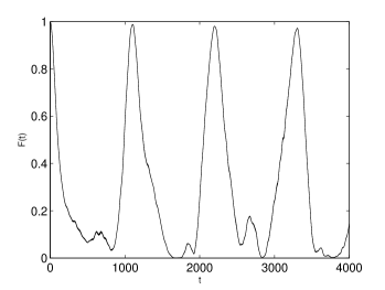
(a)

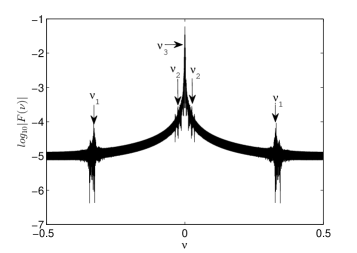
(b)

Figure 2: The fidelity for $\left(x_{0}\left(t=0\right),p_{0}\left(t=0\right)\right)=\left(0.18,0\right)$, $\beta=6\cdot 10^{-5}$ and $\tau=0.01$ (a): as function of number of kicks (b): $log_{10}|\hat{F}\left(\nu\right)|$ as a function of the inverse number of kicks $\nu$.

In Fig. 2 we found numerically that the fidelity exhibits three frequencies. A large frequency $\nu_{1}\sim 0.33\left[kicks^{-1}\right]$, corresponding to period $T_{1}\sim 3\left[kicks\right]$, an intermediate frequency, $\nu_{2}\sim 0.025\left[kicks^{-1}\right]$, corresponding to $T_{2}\sim 40\left[kicks\right]$, and a small frequency $\nu_{3}\sim 0.001\left[kicks^{-1}\right]$, corresponding to $T_{3}\sim 1000$$\left[kicks\right]$. These results were repeated for various initial values of $x_{0}\left(t=0\right)$, $p_{0}\left(t=0\right)$ and $\beta$ and are presented in Figs. 3 - 4. In Fig. 3, the periods $T_{1}$, $T_{2}$ and $T_{3}$ found from plots similar to the ones presented in Fig. 2, are plotted as a function of $\beta$ for $\left(x_{0}\left(t=0\right),p_{0}\left(t=0\right)\right)=\left(0.18,0\right)$ and $\tau=0.01$. Similar results are found for various initial conditions such that $x_{0}\left(t=0\right)\geq 0.14$, $p_{0}\left(t=0\right)=0$ and $\tau=0.01$. Note that $T_{1}$ is slowly increasing with $\beta$.

In Fig. 4, the periods $T_{1},T_{2}$ and $T_{3}$ as function of $x_{0}\left(t=0\right)$ are presented for $p_{0}\left(t=0\right)=0$, $\beta=6\cdot 10^{-5}$ and $\tau=0.01$. The results for $x_{0}\left(t=0\right)=0$, $p_{0}\left(t=0\right)\neq 0$ are similar.

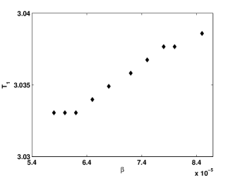
(a)

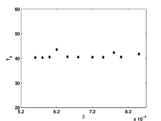
(b)

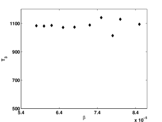
(c)

Figure 3: Various periods of the fidelity as a function of $\beta$ for $\left(x_{0}\left(t=0\right),p_{0}\left(t=0\right)\right)=\left(0.18,0\right)$ and $\tau=0.01$ (a): $T_{1}$ (b): $T_{2}$ (c): $T_{3}$

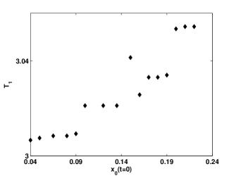
(a)

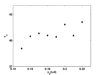
(b)

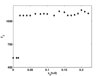
(c)

Figure 4: The various periods as a function of $x_{0}\left(t=0\right)$ for $p_{0}\left(t=0\right)=0$, $\beta=6\cdot 10^{-5}$ and $\tau=0.01$ (a): $T_{1}$ (b): $T_{2}$ (c): $T_{3}$

In all situations we found that the period $T_{1}$ varies between $3$ and $3.05$ kicks. It is very close to the value $T_{1}=\frac{2\pi}{\omega_{s}}\simeq\frac{\pi}{\omega_{1}}=3$ kicks, where $\omega_{1}$ is given by (20). The period is systematically increasing with $x_{0}\left(t=0\right)$ and $p_{0}\left(t=0\right)$ (see Fig. 4a). The reason is the deviation of the frequency from the value found in the vicinity of the fixed point at the origin. This can be verified by direct iteration of the map (11) - (12).

For $x_{0}\left(t=0\right)$ that is sufficiently large, the period $T_{3}$ was found to take the value $T_{3}\sim 1100$ kicks. It is close to value predicted from pure classical dynamics without interactions, $T_{3}=1091.8$ kicks for $K_{1}=1$ and $K_{2}=1.01$, calculated using (64). For $x_{0}\left(t=0\right)=p_{0}\left(t=0\right)=0$, we expect that $T_{3}=\frac{\pi}{\delta\omega}$, rather than $\frac{2\pi}{\delta\omega}.$ This is because of the symmetry of the initial condition. Each point of a trajectory generated by $H_{1}$ is chasing a point generated by $H_{2}$ which is its reflection through the origin of the phase space and, therefore, is found first at an angle of $\pi$ and not $2\pi$. Indeed, this was found for sufficiently small $x_{0}\left(t=0\right)$ (see Fig. 4c).

In summary, the periods $T_{1}$ and $T_{3}$ are of pure classical origin. These were found in Yevgeny_paper . Here we found that these are weakly affected by the interactions. The intermediate period $T_{2}$ is found to be $T_{2}\sim 40$ kicks (see Figs. 3b and 4b). This period was not found in absence of interactions.

We turn now to the exploration of the origin of this new period.

V The origins of the intermediate period

In this section we will demonstrate that the intermediate period results from the oscillation of the width of the wavefunction.

The Fourier transform of the width (41)

$$\hat{f}_{\Delta}\left(\nu\right)=\intop_{-\infty}^{\infty}\left\langle\Delta x\left(t\right)\right\rangle^{2}e^{-i2\pi\nu t}dt$$ (66)

was computed for $\psi$ which was derived from an initially coherent state of the form (23) by application of the evolution operator (15). We found that it exhibits the peaks $T_{1}=3.05\left[kicks\right],$ $\nu_{1}=0.328\left[\frac{1}{kick}\right]$, $\left(\omega_{1}\simeq\omega=2.06\left[\frac{1}{kick}\right]\right),$ $T_{width}=3.24$$\left[kicks\right]$ , $\nu_{width}=0.309\left[\frac{1}{kick}\right]$ and $\Omega_{width}=1.94\mbox{$\left[\frac{1}{kick}\right]$}$ for $\beta=6\cdot 10^{-5}$, $\tau=0.01$ , $\left(x_{0}\left(t=0\right),p_{0}\left(t=0\right)\right)=\left(0,0.14\right)$ and for $\left(x_{0}\left(t=0\right),p_{0}\left(t=0\right)\right)=\left(0.18,0\right)$.

We note that indeed $\Omega_{width}$ which was found numerically is close to $2\omega$. Taking $\Omega=\Omega_{width}$, we use (52) to calculate

$$\Delta\omega=2\omega-\Omega_{width},$$ (67)

and find the predicted intermediate period $T_{2}^{(p)}=\frac{2\pi}{\Delta\omega}$, where $\Omega_{width}$ is found from the numerical calculations of (66). Comparison between this value and $T_{2}$ calculated from the fidelity Fourier transform (65) is shown in Fig. 5. The difference is small, as expected from section III.3.

An obvious question is how is it possible that an oscillation with the same period $T_{2}$ is found for all $\beta\neq 0$, but no such oscillation is found for $\beta=0$. For this purpose, the amplitude of this oscillation Fourier transform peak $\hat{f_{2}}$ as function of $\beta$ is plotted in Fig. 6. It can be seen that the amplitude decreases as $\beta$ decreases.

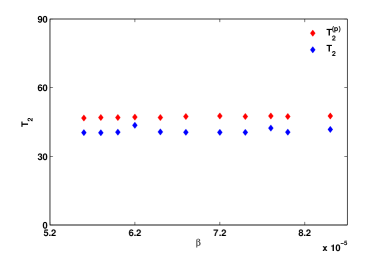
Figure 5: (Color online) The predicted intermediate period of the fidelity $T_{2}^{(p)}$ compared to $T_{2}$, found directly from the Fourier transform of the fidelity, as function of $\beta$, for $\left(x_{0}\left(t=0\right),p_{0}\left(t=0\right)\right)=\left(0.18,0\right)$ and $\tau=0.01$ .

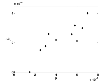
Figure 6: Fidelity Fourier transform amplitude of $f_{2}$ as function of $\beta$ for $\tau=0.01$, $\left(x_{0}\left(t=0\right),p_{0}\left(t=0\right)\right)=\left(0.18,0\right)$ and $7000$ kicks

The generation of the intermediate period is not characteristic of the fidelity but will show up in any correlation function involving overlap of Wigner functions. The fidelity is the overlap of Wigner functions at the same time but different Hamiltonians. Similar behavior is found for overlap of the Wigner functions for the same Hamiltonian but at different times $n$ and $n-\Delta n$ defined by

$$G\left(n\right)=\iintop_{-\infty}^{\infty}W_{n}\left(x,p\right)W_{n-\Delta n}\left(x,p\right)dxdp$$ (68)

and calculated in detail in Appendix B.

First, we note that the Wigner function rotates around the elliptic point as demonstrated in Fig. 7 for 990-995 kicks. In Fig. 7a we see that for $\beta=0$ the function shape is smeared over the phase space. In Fig. 7b we see that the Wigner function for $\beta\neq 0$ is localized due to the interactions. Hence, in this case interactions tend to localize the Wigner function in phase space. In presence of interactions the general form is indeed (26) with (42) and (44), replacing $\sigma_{x_{i}}^{2}$ and $\sigma_{p_{i}}^{2}$, respectively.

The Fourier transform of the correlation function $G\left(n\right)$ and the Fourier transform of the fidelity with the same parameters as in Fig. 2 have been compared. The intermediate frequency found from the fidelity is $\nu_{2}=0.025\left[kicks^{-1}\right]$ , $\omega_{2}=0.157\left[\frac{1}{kick}\right]$ with period $T_{2}=40.57\left[kicks\right]$, and the frequency found from $G\left(n\right)$ is $\nu_{2}=0.024\left[kicks^{-1}\right]$ with $\omega_{2}=0.151\left[\frac{1}{kick}\right]$ and $T_{2}=42.52\left[kicks\right]$. The results are similar in both cases.

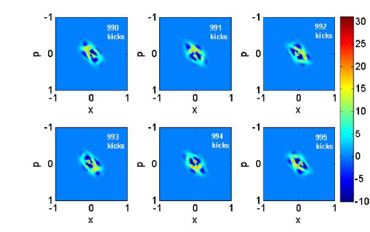
(a)

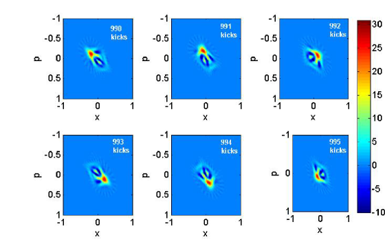
(b)

Figure 7: (Color online) The Wigner function for 990 - 995 kicks for $\left(x_{0},p_{0}\right)=\left(0.18,0\right)$, $\beta=6\cdot 10^{-5}$ and $\tau=0.01.$ (a): $\beta=$0, (b): $\beta=6\cdot 10^{-5}$.

VI Summary and discussion

The effects of weak inter-particle interactions on the quantum fidelity were calculated for kicked particles. The calculation was performed for a specific model where the interaction was introduced during the kicks. The results were found to be qualitatively similar to the ones found where the interactions were introduced between kicks Mark_Update . We found that the periods that were obtained in absence of the interactions, namely, $T_{1}$ and $T_{3}$, are found also in the presence of the interactions. In presence of the interactions, another period, namely, $T_{2}$, was found. We explored the mechanism of the generation of this frequency. It results of the interplay of the oscillations of the width of the wave function (or Wigner function) in phase space and the rotation of its center around the elliptic fixed point. It is $\Delta\omega$ of (52) that was derived in the framework of the heuristic model outlined in Sec. III and tested numerically in Sec. V. In Fig. 7 it was verified that the heuristic picture of Sec. III holds for the kicked model presented in the introduction. The frequencies found in this work for the fidelity are found also for other correlation functions of Wigner functions.

In this work we focused on dynamics of wave packets in the vicinity of the elliptic fixed point $\left(x,p\right)=\left(0,0\right)$ for the classical phase portrait shown in Fig. 1.

The existence of the intermediate frequency $\Delta\omega$ ((52)) and its origin is the main result of this paper. From the analysis of Mark_paper it is plausible that the origin of this frequency is semiclassical. The meaning is that the term $\beta\left|\psi\left(x\right)\right|^{2}$ in (13), (15) and (16) acts as a potential. The intermediate frequency is not found numerically if the center of the wave packet is too close to the elliptic fixed point. A possible explanation is that in such a situation one does not have the possibility to separate the rotations of the center of the packet and the oscillation of the width.

As one increases the distance of the wave packet from the fixed point at the origin while keeping the nonlinearity fixed, the variation of the rotation frequency increases and the packet spreads over a ring in phase space, as is the case for $\beta=0$ (see Fig. 7a). In such a situation the picture of Sec. III is violated. Nevertheless, the same intermediate frequency $\Delta\omega$ is numerically found. This should be left for further studies.

Appendix A Fidelity calculation details

The equations (46) and (47) are simplified by means of a Taylor expansion

$$\frac{1}{1-x}\simeq 1+x+O\left(x^{2}\right),$$ (69)

combined with

$$\cos\alpha\cdot\cos\beta=\frac{1}{2}\left(\cos\left(\alpha-\beta\right)+\cos\left(\alpha+\beta\right)\right),$$ (70)

the equations take the form

$$s_{x} = \frac{\rho^{2}}{2\sigma_{x}^{2}}-\frac{\rho^{2}}{2\sigma_{x}^{2}}\cos\left(\delta\omega\cdot t\right)+\frac{\rho^{2}\nu}{4\sigma_{x}^{4}}\cos\left(\left(\Omega-\delta\omega\right)t+\phi_{x}\right)$$

$$+\frac{\rho^{2}\nu}{4\sigma_{x}^{4}}cos\left(\left(\Omega+\delta\omega\right)t+\phi_{x}\right)-\frac{\rho^{2}\nu}{2\sigma_{x}^{4}}\cos\left(\Omega\cdot t+\phi_{x}\right)$$

and

$$s_{p} = \frac{\rho^{2}m^{2}\omega^{2}}{2\sigma_{p}^{2}}-\frac{\rho^{2}m^{2}\omega^{2}}{\sigma_{p}^{2}}\cos\left(2\omega\cdot t\right)+\frac{\rho^{2}m^{2}\omega^{2}}{2\sigma_{p}^{2}}\cos\left(\delta\omega\cdot t\right)+$$

$$+\frac{\rho^{2}m^{2}\gamma\omega^{2}}{2\sigma_{p}^{4}}\cos\left(\left(2\omega+\Omega\right)t+\phi_{p}\right)-\frac{\rho^{2}m^{2}\gamma\omega^{2}}{4\sigma_{p}^{4}}\cos\left(\left(\Omega-\delta\omega\right)t+\phi_{p}\right)$$

$$-\frac{\rho^{2}m^{2}\gamma\omega^{2}}{4\sigma_{p}^{4}}\cos\left(\left(\Omega+\delta\omega\right)t+\phi_{p}\right)+\frac{\rho^{2}m^{2}\gamma\omega^{2}}{2\sigma_{p}^{4}}\cos\left(\left(2\omega+\Omega\right)t+\phi_{p}\right)$$

$$-\frac{\rho^{2}m^{2}\gamma\omega^{2}}{4\sigma_{p}^{4}}\cos\left(\left(\Omega-\delta\omega\right)t+\phi_{p}\right)-\frac{\rho^{2}m^{2}\gamma\omega^{2}}{4\sigma_{p}^{4}}\cos\left(\left(\Omega+\delta\omega\right)t+\phi_{p}\right)+$$

$$+\frac{\rho^{2}m^{2}\gamma\omega^{2}}{2\sigma_{p}^{4}}\cos\left(\Delta\omega-\phi_{p}\right)-\frac{\rho^{2}m^{2}\gamma\omega^{2}}{2\sigma_{p}^{4}}\cos\left(\Omega\cdot t+\phi_{p}\right).$$

From this, one finds (53) - (61).

Appendix B Correlation of the Wigner function at various times

In this Appendix we identify the frequencies of $G\left(n\right)$ defined by (68), where $\Delta n$ is fixed. The derivation is similar to the derivation of the fidelity oscillations is Sec. III and Appendix A. First, we assume there are no interactions and then we add the effect of weak interactions. We consider wave packets near the elliptic fixed point $\left(x,p\right)=\left(0,0\right)$ and as in the case of the fidelity we calculate $G\left(n\right)$ in continuous time for a harmonic well.

B.1 Correlation of Wigner functions for different times in absence of interactions

Let $\omega_{1}$ be the frequency of a harmonic oscillator. The Wigner function of a coherent state of the oscillator (23), corresponding to a time $t$ is (26), namely

$$W_{t}\left(x,p\right)=\frac{1}{2\pi\sigma_{x}\sigma_{p}}e^{-\frac{1}{2}\left(\frac{\left(x-x\left(t\right)\right)^{2}}{\sigma_{x}^{2}}+\frac{\left(p-p\left(t\right)\right)}{\sigma_{p}^{2}}\right)}.$$ (73)

The Wigner function corresponding to a time $t-\Delta t$ is

$$W_{t-\Delta t}\left(x,p\right)=\frac{1}{2\pi\sigma_{x}\sigma_{p}}e^{-\frac{1}{2}\left(\frac{\left(x-x\left(t-\Delta t\right)\right)^{2}}{\sigma_{x}^{2}}+\frac{\left(p-p\left(t-\Delta t\right)\right)^{2}}{\sigma_{p}^{2}}\right)},$$ (74)

where $\sigma_{x}$ and $\sigma_{p}$ are given by (27) and (28) and denote the width of the Wigner function in position and momentum, respectively. The difference between the times is constant and given by $\Delta t.$

The correlation in absence of interactions is of the form

$$G=C\cdot e^{-\frac{1}{2}\left(s_{x}+s_{p}\right)}$$ (75)

with

$$C=\frac{1}{4\pi\sigma_{x}\sigma_{p}},$$ (76)

$$s_{x}=\frac{\left(x\left(t\right)-x\left(t-\Delta t\right)\right)^{2}}{2\sigma_{x}^{2}}$$ (77)

and

$$s\left(p\right)=\frac{\left(p\left(t\right)-p\left(t-\Delta t\right)\right)^{2}}{2\sigma_{p}^{2}}.$$ (78)

The phase coordinates are

$$\left(x\left(t\right),p\left(t\right)\right)=\rho\left(\cos\left(\omega t\right),-m\omega\sin\left(\omega t\right)\right)$$ (79)

and

$$\left(x\left(t-\Delta t\right),p\left(t-\Delta t\right)\right)=\rho\left(\cos\left(\omega t+\phi\right),-m\omega\sin\left(\omega t+\phi\right)\right),$$ (80)

where

$$\phi=\omega\Delta t.$$ (81)

B.2 Correlation of Wigner functions for different times with weak interactions

The width of the Wigner functions in presence of weak interactions is given by

$$\tilde{\sigma}_{x_{1}}^{2}=\sigma_{x}^{2}+\gamma_{x}\cos\left(\Omega t+\phi_{x}\right),$$ (82)

$$\tilde{\sigma}_{x_{2}}=\sigma_{x}^{2}+\gamma_{x}\cos\left(\Omega t+\phi_{x}-\Delta\phi\right),$$ (83)

$$\tilde{\sigma}_{p_{1}}=\sigma_{p}^{2}+\gamma_{p}\cos\left(\Omega t+\phi_{p}\right)$$ (84)

and

$$\tilde{\sigma}_{p_{2}}^{2}=\sigma_{p}^{2}+\gamma_{p}\cos\left(\Omega t+\phi_{p}-\Delta\phi\right),$$ (85)

where

$$\Delta\phi=\Omega\cdot\Delta t.$$ (86)

Therefore,

$$C\left(t\right)=\left(2\pi\sigma_{x\left(t\right)}\sigma_{p\left(t\right)}\sigma_{x\left(t-\Delta t\right)}\sigma_{p\left(t-\Delta t\right)}\right)^{-1}\sqrt{\frac{\sigma_{x\left(t\right)}^{2}\sigma_{x\left(t-\Delta t\right)}^{2}\sigma_{p\left(t\right)}^{2}\sigma_{p\left(t-\Delta t\right)}^{2}}{\left(\sigma_{x\left(t\right)}^{2}+\sigma_{x\left(t-\Delta t\right)}^{2}\right)\left(\sigma_{p\left(t\right)}^{2}+\sigma_{p\left(t-\Delta t\right)}^{2}\right)}}$$ (87)

and

$$G\left(t\right)=C\left(t\right)\cdot e^{-\frac{1}{2}\left(s_{x}\left(t\right)+s_{p}\left(t\right)\right)}.$$ (88)

The expressions for $s\left(x\right)$ and $s\left(p\right)$ become

$$s_{x}\left(t\right)=\frac{\rho^{2}}{2\sigma_{x}^{2}}\cdot\frac{\left(\cos\left(\omega t\right)-\cos\left(\omega t-\phi\right)\right)^{2}}{1+\gamma_{x}\left(\cos\left(\Omega t+\phi_{x}\right)+\cos\left(\Omega t+\phi_{x}-\Delta\phi\right)\right)}$$ (89)

and

$$s_{p}\left(t\right)=\frac{\rho^{2}m^{2}\omega^{2}}{2\sigma_{p}^{2}}\cdot\frac{\left(\sin\left(\omega t\right)-\sin\left(\omega t-\phi\right)\right)^{2}}{1+\gamma_{x}\left(\cos\left(\Omega t+\phi_{p}\right)+\cos\left(\Omega t+\phi_{p}-\Delta\phi\right)\right)}.$$ (90)

Using (70), we get

$$s_{x}\left(t\right)=\sum_{i=1}^{8}A_{i},$$ (91)

where

$$A_{1}=\frac{\rho^{2}}{2\sigma_{x}^{2}}-\frac{\rho^{2}\gamma_{x}}{2\sigma_{x}^{2}}\cos\left(\Omega t+\phi_{x}\right)-\frac{\rho^{2}\gamma_{x}}{2\sigma_{x}^{2}}\cos\left(\Omega t+\phi_{x}-\Delta\phi\right),$$ (92)

$$A_{2}=\frac{\rho^{2}}{4\sigma_{x}^{2}}\cos\left(2\omega t\right)+\frac{\rho^{2}}{4\sigma_{x}^{2}}\cos\left(2\omega t-2\phi\right)-\frac{\rho^{2}}{2\sigma_{x}^{2}}\cos\left(\phi\right)\cos\left(2\omega t-\phi\right),$$ (93)

$$A_{3}=-\frac{\rho^{2}\gamma_{x}}{8\sigma_{x}^{2}}\cos\left(\left(2\omega-\Omega\right)t-\phi_{x}\right)-\frac{\rho^{2}\gamma_{x}}{8\sigma_{x}^{2}}\cos\left(\left(2\omega-\Omega\right)t-\phi_{x}+\Delta\phi\right),$$ (94)

$$A_{4}=-\frac{\rho^{2}\gamma_{x}}{8\sigma_{x}^{2}}\cos\left(\left(2\omega-\Omega\right)t-2\phi-\phi_{x}+\Delta\phi\right)+\frac{\rho^{2}\gamma_{x}}{4\sigma_{x}^{2}}\cos\left(\left(2\omega-\Omega\right)t-\phi-\phi_{x}\right),$$ (95)

$$A_{5}=\frac{\rho^{2}\gamma_{x}}{4\sigma_{x}^{2}}\cos\left(\phi\right)\cos\left(\left(2\omega-\Omega\right)t-\phi-\phi_{x}+\Delta\phi\right)-\frac{\rho^{2}\gamma_{x}}{8\sigma_{x}^{2}}\cos\left(\left(2\omega-\Omega\right)t-2\phi-\phi_{x}\right),$$ (96)

$$A_{6}=-\frac{\rho^{2}\gamma_{x}}{8\sigma_{x}^{2}}\cos\left(\left(2\omega+\Omega\right)t+\phi_{x}\right)-\frac{\rho^{2}\gamma_{x}}{8\sigma_{x}^{2}}\cos\left(\left(2\omega+\Omega\right)t+\phi_{x}-\Delta\phi\right),$$ (97)

$$A_{7}=-\frac{\rho^{2}\gamma_{x}}{8\sigma_{x}^{2}}\cos\left(\left(2\omega+\Omega\right)t-2\phi+\phi_{x}\right)-\frac{\rho^{2}\gamma_{x}}{8\sigma_{x}^{2}}\cos\left(\left(2\omega+\Omega\right)t-2\phi+\phi_{x}-\Delta\phi\right)$$ (98)

and

$$A_{8}=\frac{\rho^{2}\gamma_{x}}{4\sigma_{x}^{2}}\cos\left(\phi\right)\cos\left(\left(2\omega+\Omega\right)t-\phi+\phi_{x}\right)+\frac{\rho^{2}\gamma_{x}}{4\sigma_{x}^{2}}\cos\left(\phi\right)\cos\left(\left(2\omega+\Omega\right)t-\phi+\phi_{x}-\Delta\phi\right).$$ (99)

The intermediate frequency is present in (94) - (96) and is equal to $\Delta\omega=2\omega-\Omega.$

Similarly, for $s_{p}\left(t\right)$,

$$s_{p}\left(t\right)=\sum_{i=1}^{8}A_{i},$$ (100)

where

$$A_{1}=\frac{\rho^{2}m^{2}\omega^{2}}{2\sigma_{p}^{2}}\left(1-\cos\left(\phi\right)\right)-\frac{\rho^{2}m^{2}\omega^{2}\gamma_{p}}{2\sigma_{p}^{2}}\cos\left(\Omega t+\phi_{p}\right)-\frac{\rho^{2}m^{2}\omega^{2}\gamma_{p}}{2\sigma_{p}^{2}}\cos\left(\Omega t+\phi_{p}-\Delta\phi\right),$$ (101)

$$A_{2}=\frac{\rho^{2}m^{2}\omega^{2}\gamma_{p}}{2\sigma_{p}^{2}}\cos\left(\phi\right)\cos\left(\Omega t+\phi_{p}\right)+\frac{\rho^{2}m^{2}\omega^{2}\gamma_{p}}{2\sigma_{p}^{2}}\cos\left(\phi\right)\cos\left(\Omega t+\phi_{p}-\Delta\phi\right),$$ (102)

$$A_{3}=-\frac{\rho^{2}m^{2}\omega^{2}}{2\sigma_{p}^{2}}\cos\left(2\omega t\right)-\frac{\rho^{2}m^{2}\omega^{2}}{2\sigma_{p}^{2}}\cos\left(2\omega t+2\phi\right)+\frac{\rho^{2}m^{2}\omega^{2}}{2\sigma_{p}^{2}}\cos\left(2\omega t+\phi\right),$$ (103)

$$A_{4}=\frac{\rho^{2}m^{2}\omega^{2}\gamma_{p}}{4\sigma_{p}^{2}}\cos\left(\left(2\omega-\Omega\right)t-\phi_{p}\right)+\frac{\rho^{2}m^{2}\omega^{2}\gamma_{p}}{4\sigma_{p}^{2}}\cos\left(\left(2\omega-\Omega\right)t-\phi_{p}+\Delta\phi\right),$$ (104)

$$A_{5}=\frac{\rho^{2}m^{2}\omega^{2}\gamma_{p}}{4\sigma_{p}^{2}}\cos\left(\left(2\omega-\Omega\right)t+2\phi-\phi_{p}\right)+\frac{\rho^{2}m^{2}\omega^{2}\gamma_{p}}{4\sigma_{p}^{2}}\cos\left(\left(2\omega-\Omega\right)t+2\phi-\phi_{p}+\Delta\phi\right),$$ (105)

$$A_{6}=-\frac{\rho^{2}m^{2}\omega^{2}\gamma_{p}}{4\sigma_{p}^{2}}\cos\left(\left(2\omega-\Omega\right)t+\phi-\phi_{p}\right)-\frac{\rho^{2}m^{2}\omega^{2}\gamma_{p}}{4\sigma_{p}^{2}}\cos\left(\left(2\omega-\Omega\right)t+\phi-\phi_{p}\Delta\phi\right),$$ (106)

$$A_{7}=\frac{\rho^{2}m^{2}\omega^{2}\gamma_{p}}{4\sigma_{p}^{2}}\cos\left(\left(2\omega+\Omega\right)t+\phi_{p}\right)+\frac{\rho^{2}m^{2}\omega^{2}\gamma_{p}}{4\sigma_{p}^{2}}\cos\left(\left(2\omega+\Omega\right)t+\phi_{p}-\Delta\phi\right),$$ (107)

$$A_{8}=\frac{\rho^{2}m^{2}\omega^{2}\gamma_{p}}{4\sigma_{p}^{2}}\cos\left(\left(2\omega+\Omega\right)t+2\phi+\phi_{p}\right)+\frac{\rho^{2}m^{2}\omega^{2}\gamma_{p}}{4\sigma_{p}^{2}}\cos\left(\left(2\omega+\Omega\right)t+2\phi+\phi_{p}-\Delta\phi\right)$$ (108)

and

$$A_{9}=-\frac{\rho^{2}m^{2}\omega^{2}\gamma_{p}}{4\sigma_{p}^{2}}\cos\left(\left(2\omega+\Omega\right)t+\phi+\phi_{p}\right)-\frac{\rho^{2}m^{2}\omega^{2}\gamma_{p}}{4\sigma_{p}^{2}}\cos\left(\left(2\omega+\Omega\right)t+\phi+\phi_{p}-\Delta\phi\right).$$ (109)

The intermediate frequency $\Delta\omega=2\omega-\Omega$ can be seen in (104) - (106).

References

- (1) L.Rebuzzini, R.Artuso, S.Fishman, and I. Guarneri, “Effects of atomic interactions on quantum accelerator modes,” Phys. Rev. A, vol. 76, 031603(R), 2007.
- (2) C. Zhang, J. Liu, M. G.Raizen, and Q. Niu, “Transition to instability in a kicked bose-einstein condensate,” Phys. Rev. Lett., vol. 92, p. 054101, 2004.
- (3) S.Moulieras, A.G.Monastra, M.Saraceno, and P.Leboeuf, “Wave-packet dynamics in nonlinear schrodinger equations,” Phys. Rev. A, vol. 85, 013841, 2012.
- (4) M.Herrera, T.M.Antonsen, E.Ott, and S.Fishman, “Dynamic localization of a weakly interacting bose-einstein condensate in an anharmonic potential,” Phys. Rev. A, vol. 87,041603(R), 2013.
- (5) A.Peres, “Stability of quantum motion in chaotic and regular systems,” Phys. Rev. A, vol. 30, 1610, 1984.
- (6) R.A.Jalabert and H.M.Pastawski, “Environmental-independent decoherence rate in classically chaotic systems,” Phys. Rev. Lett., vol. 86, 2490, 2001.
- (7) P.Jacquod, I.Adagideli, and C.W.J.Beenakker, “Decay of the loschmidt echo for quantum states with sub-planck-scale structures,” Phys. Rev. Lett., vol. 89, 154103, 2002.
- (8) N.R.Cerruti and S.Tomsovic, “Sensitivity of wave field evolution and manifold stability in chaotic systems,” Phys. Rev. Lett., vol. 88, 054103, 2002.
- (9) S.Wimberger and A. Buchleitner, “Saturation of fidelity in the atom-optics kicked rotor,” J. Phys. B, vol. 39, L145, 2006.
- (10) M.F.Andersen, A.Kaplan, T. Grunzweig, and N.Davidson, “Decay of quantum correlations in atom optic billiards with chaotic and mixed dynamics,” Phys. Rev. Lett., vol. 97, 104102, 2006.
- (11) A.Kaplan, M.Andersen, T.Grunzweig, and N.Davidson, “Hyperfine spectroscopy of optically trapped atoms,” J. Opt. B, vol. 7, R103, 2005.
- (12) M.F.Andersen, T.Grunzweig, A.Kaplan, and N.Davidson, “Revivals of coherence in chaotic atom-optics billiards,” Phys. Rev. A, vol. 69, 063413, 2004.
- (13) T.Gorin, T.Prosen, T.H.Seligman, and M.Znidaric, “Dynamics of loschmidt echoes and fidelity decay,” Phys. Rep., vol. 435, 33, 2006.
- (14) Y. Krivolapov, S. Fishman, E. Ott, and T. M. Antonsen, “Quantum chaos of a mixed open system of kicked cold atoms,” Phys. Rev. E, vol. 83,016204, 2011.
- (15) M.Herrera, “private communication,” april 2013.
- (16) D.L.Shepelyansky, “Delocalization of quantum chaos by weak nonlinearity,” Phys. Rev. Lett., vol. 70, 1787, 1993.
- (17) M.Herrera, T.M.Antonsen, E.Ott, and S.Fishman, “Echoes and revival echoes in systems of anharmonically confined atoms,” Phys. Rev. A, vol. 86,023613, 2012.
- (18) P.Milloni and M.Nieto, “Coherent states,” in Compendium of Quantum Physics, D. Greenberger, K. Hentschel, and F. Weinert, Eds. Springer Berlin Heidelberg, 2009, pp. 106–108.