The Evolution of High Temperature Plasma in Magnetar Magnetospheres and its Implications for Giant Flares

Abstract

In this paper we propose a new mechanism describing the initial spike of giant flares in the framework of the starquake model. We investigate the evolution of a plasma on a closed magnetic flux tube in the magnetosphere of a magnetar in the case of a sudden energy release and discuss the relationship with observations of giant flares. We perform one-dimensional numerical simulations of the relativistic magnetohydrodynamics in Schwarzschild geometry. We assume energy is injected at the footpoints of the loop by a hot star surface containing random perturbations of the transverse velocity. Alfvén waves are generated and propagate upward, accompanying very hot plasma that is also continuously heated by nonlinearly generated compressive waves. We find that the front edges of the fireball regions collide at the top of the tube with their symmetrically launched counterparts. This collision results in an energy release which can describe the light curve of initial spikes of giant flares.

1. Introduction

Soft gamma-ray repeaters (SGRs) and anomalous X-ray pulsars (AXPs) have been considered to be strongly magnetized astrophysical objects. Recent X-ray observations have shown that SGRs and AXPs have similar luminosity, pulse period, period derivative, and burst activity, so that they are considered to belong to the same population, called “magnetars” which are isolated neutron stars powered by the dissipation of magnetic field energy (Duncan & Thompson, 1992; Harding & Lai, 2006). Their typical period is $P\sim 10$ [s] and period derivative is $\dot{P}\sim 10^{-10}$ to $10^{-12}$ [s/s], which indicates that their magnetic field is about $B\geq 10^{13}$ [G] (Woods & Thompson, 2006; Mereghetti, 2008). Concerning their X-ray spectra, they indicate that AXPs and SGRs have a blackbody component with temperature $k_{B}T\sim 0.5$ [keV] (Mereghetti et al., 2002, 2005, 2006), and $k_{B}T\sim 5-10$ [keV] in the case of SGRs in their active phase (Feroci et al., 2004; Olive et al., 2004; Nakagawa et al., 2007; Esposito et al., 2007).

Giant flares cause the sudden release of an enormous amount of energy $\sim 10^{44}$ [erg] (e.g. Tanaka et al. (2007)), and they have been observed from SGRs. Their spectra and temporal evolution consist of a short hard spike followed by a pulsating tail. The rise-time of the spike is about one milli-second, its duration is about $0.1$ [s], and its temperature is about $240$ [keV] (e.g. Hurley et al. (2005)), respectively. The tail has coherent pulsations, presumably at the spin period of the underlying neutron star. It has a softer spectra and gradually decays in hundreds of seconds. The total amount of energy of the tail is about $10^{44}$ [erg], which is believed to be the energy trapped in the magnetosphere.

The physical mechanism of giant flares is still unclear and there are a lot of investigations  (Thompson & Duncan, 1995; Thompson et al., 2002; Lyutikov, 2003, 2006; Masada et al., 2010; Parfrey et al., 2013). One of the most popular mechanisms is magnetic reconnection, which is a process that converts magnetic field energy into the plasma thermal and kinetic energy rapidly  (Lyutikov & Uzdensky, 2003; Lyutikov, 2003; Lyubarsky, 2005; Lyutikov, 2006; Zenitani et al., 2010; Takamoto, 2013). Hence, it allows to convert the strong magnetic field energy of magnetars into radiation. In particular, the twisted magnetic flux rope model (Lyutikov, 2006; Gill & Heyl, 2010; Yu, 2012; Yu & Huang, 2013) is recently considered to be a promising candidate for magnetar flare phenomena because the twisted component allows to trigger various kinds of plasma instabilities (e.g. Török et al. (2004); Kliem & Török (2006)). Although magnetic reconnection has many attractive properties, it is subject to uncertainties which include its typical growing timescale and its energy conversion rate into radiation which relate to the precise mechanism of the eruption. In addition, little is known about the global magnetic field structure in the magnetar magnetosphere  (Beloborodov & Thompson, 2007; Beloborodov, 2009; Takamori et al., 2012; Beloborodov, 2013; Parfrey et al., 2013), which always plays a crucial role in the formation of the current sheets needed for magnetic reconnection.

It is widely known that the flares are ubiquitous on the Sun. Masada et al. (2010) pointed out that there are a lot of similarities between magnetar giant flares and solar flares, and constructed a theoretical model based on the solar flare. Even though there may be differences between the magnetar magnetosphere and the solar atmosphere, we think that the physical understanding of solar flares can be fruitfully applied to research on magnetar giant flares. Referring to numerical simulations of solar coronal loops by Moriyasu et al. (2004), transient flare-like events are frequently seen even though quasi-steady Alfvénic perturbations are injected from the footpoints of a 1D closed flux tube. This is interpreted as a consequence of nonlinear interaction of counter-propagating waves. We expect that such a mechanism possibly operates in closed loops on a magnetar.

In this paper, we propose a new mechanism describing the initial spike based on the starquake model  (Pacini, 1974; Blaes et al., 1989; Thompson & Duncan, 1995, 1996; Kojima & Okita, 2004; Piro, 2005; Okita et al., 2008; Mazur & Heyl, 2011; Gabler et al., 2012), which considers an excitation of magnetic field oscillations by the energy release of crust elastic energy through a starquake. We consider the evolution of fireball region along a magnetic flux tube using the general relativistic magnetohydrodynamic (GRMHD) approximation. In addition, we consider Alfvén waves driven on the star surface and study their effects on the plasma evolution. In our model, the fireball region expands along a magnetic flux tube and collides to the counterpart that propagates from the other side of the tube as indicated in Figure 1, which can result in the initial spike of giant flares. This short timescale of the collision enables us to explain the timescale of the initial spike even in the framework of the starquake model. Because of the heating by Alfvén waves, the front edge of the region keeps its internal energy, so that the induced energy is large enough to explain the observed energy of initial spikes.

This paper is organized as follows: In section 2, we explain the numerical set up and also give the basic equations. In section 3, the numerical results are presented; in addition, we present the new mechanism of the initial spike. In section 4, we give several comments on the relation to the observations.

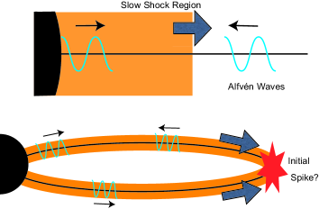
Figure 1.— A schematic picture of a mechanism generating the initial spike of the giant flare through the collision of slow shocks. The black lines are the magnetic field line; the orange regions are the post shock region of slow shocks; the blue wavy lines are the Alfvén waves.

2. Method

2.1. Numerical Setup

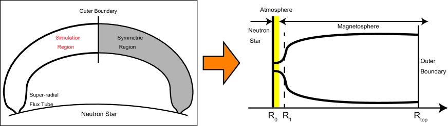
Figure 2.— Schematic pictures of a flux tube with the super-radial expansion structure. Left: A global picture of the flux tube. Right: A local picture of the flux tube of simulation region along its central line. The left-hand region is the neutron star; the yellow region is the atmosphere; $r=R_{1}$ is the coordinate where the flux tube expands mainly; the right-hand region is the magnetosphere.

We model the evolution of a plasma in a magnetar magnetosphere using the general relativistic magnetohydrodynamic (GRMHD) approximation in Schwarzschild spacetime with Schwarzschild radius $r_{g}=0.3R_{0}$ where $R_{0}\sim 10^{6}$[cm] is the neutron star radius. In particular, we focus on the temporal evolution of the plasma along a closed magnetic field line. We set up one-dimensional closed magnetic flux tubes (Figure 2) whose structure is fixed during our simulations . The simulation region is from the surface ($r=R_{0}$) to the loop top that is located at $r=R_{\mathrm{top}}$ where $R_{\mathrm{top}}$ is the radial coordinate of the loop top. We assume the mirror symmetry across the loop top and prescribe the reflection boundary condition there. From the surface, we inject transverse velocity perturbations which excite Alfvén waves. To simplify the numerical modeling, we assume that the gravitational force is parallel to the flux tube. Although this approximation is not very good near the loop top, the gravitational force there is considerably weaker than in the near-surface region. Therefore, this approximation does not affect so much the overall trends of the evolution of the plasma in the magnetosphere.

In order to model general configurations of closed magnetic loops, we introduce a super-radial expansion factor, $f(r)$, which was originally adopted to treat open magnetic flux tubes on the Sun (Kopp & Holzer, 1976). The solar surface is occupied by many small-scale closed loops, and as a result, open magnetic flux tubes rapidly expand around the height of these small loops, which is actually observed on the Sun (Tsuneta et al., 2008; Ito et al., 2010). We expect that the large-scale magnetic loops, which we are now considering, would have similar structure. We adopt the same functional form,

$$f(r)=\frac{f_{\mathrm{Max}}\exp\left[(r-R_{1})/\Sigma\right]+f_{1}}{\exp\left[(r-R_{1})/\Sigma\right]+1},$$ (1)

where $f_{\mathrm{Max}}$ is the total expansion factor, and the value of $f_{1}$ is determined so as to satisfy $f(R_{0})=1$ . $f(r)$ changes its value mainly at $r=R_{1}$, within the region between $R_{1}-\Sigma$ and $R_{1}+\Sigma$. We perform simulations in the super-radial expanding flux tubes with $f_{\mathrm{Max}}=7.5$ and in the purely radial expanding case ($f_{\mathrm{Max}}=1$). Throughout the paper, we adopt $\Sigma=0.05R_{0}$ and $R_{1}=1.1R_{0}$ that is of the same order of the scale height. Then, from the conservation of radial magnetic flux, the radial magnetic field strength can be fixed as

$$B^{r}r^{2}f(r)=\mathrm{const.},$$ (2)

where $r$ is the coordinate measured along the flux tube.

We divide the numerical domain into homogeneous numerical meshes with $\Delta_{r}=10^{-3}R_{0}$. Regarding the inner boundary, mass inflow into the simulation domain is allowed, which results from evaporation of the star surface due to a starquake that triggers giant flares; in addition, we consider transverse velocity fluctuations excited by random motions on the star surface with a power law spectrum indicated in the solar activity (Matsumoto & Kitai, 2010), $P(\nu)\propto\nu^{-1}$, where $\nu$ is the oscillation frequency, which produces linearly polarized Alfvén waves in the atmosphere and magnetosphere region. Basically, we use the average velocity, $\langle\delta v_{\perp}\rangle/c_{s,r}=0.1,0.5,0.75,0.9$ where $c_{s,r}=c/\sqrt{3}$ is the relativistic sound velocity. We resolve an Alfvén wave by at least $100$ grids per wavelength whose frequency is approximately $10c_{A}/R_{0}$ where $c_{A}$ is the Alfvén velocity. We discuss the validity of the assumed Alfvén wave properties in Section 4.3.

In this paper, we consider a relativistically hot magnetar surface heated by some burst phenomena, such as a starquake. At the initial time, we assume there are three regions: the star surface, the atmosphere and the plasma in the magnetosphere, as shown in the Figure 2. At $r=R_{0}$, we consider the star surface as the inner boundary explained above. In the region close to the star surface, $R_{0}<r<1.005R_{0}$   , we assume there is an atmosphere heated by the central star surface with a fixed temperature $T=50$ [keV] which is observed in the case of the initial spike of giant flares (Woods & Thompson, 2006; Mereghetti, 2008). In the region outside of the atmosphere, $1.005R_{0}<r<R_{\mathrm{top}}$, we consider the plasma in the magnetosphere with temperature is $T=7.5$ [keV] which is equivalent to the persistent blackbody component of the observed X-ray spectrum of magnetars. Note that the temperature of the plasma outside of the atmosphere is heated by various waves and shocks and changes its value as shown in the numerical results. The initial structure of the plasma outside of the atmosphere is determined using hydrostatic equilibrium of an isothermal plasma. Concerning the magnetization parameter $\sigma\equiv B^{2}/4\pi\rho h\gamma^{2}c^{2}v$ where $\rho$ is the rest mass density, $h$ is the specific enthalpy, and $\gamma$ is the Lorentz factor, we consider a moderately magnetized plasma, $\sigma=2$ at the inner edge of the high temperature atmosphere, and $\sigma=10$ at just outside of the atmosphere. Even though these values are too small for the magnetar magnetosphere (Thompson & Duncan, 1995), we believe that our findings are still be applicable to the magnetar flare phenomena. We will discuss it in Section 4.

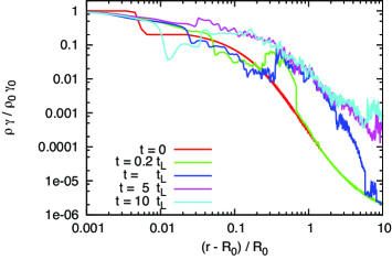
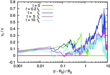
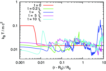
Figure 3.— The snapshots of the temperature profile $k_{B}T/mc^{2}$, density profile in the laboratory frame $\rho\gamma$, and radial velocity $v_{r}$ at $t/t_{L}=0,0.2,1,5,10$ where $t_{L}=10t_{0}\equiv 10R_{0}/c$ is the light crossing time along the loop.

2.2. Basic Equation

As we mentioned above, we solve the dynamical evolution of the plasma and waves by solving the ideal GRMHD equations in Schwarzschild spacetime:

$$ds^{2} = g_{\mu\nu}dx^{\mu}dx^{\nu},$$

$$= -w(r)dt^{2}+w(r)^{-1}dr^{2}+r^{2}(d\theta^{2}+\sin^{2}\theta d\phi^{2}),$$

where $w(r)=1-r_{g}/r$, $r_{g}\equiv 2MG/c^{2}$ is the Schwarzschild radius, $M,G,c$ are the central star mass, the gravitational constant and the light velocity, respectively. We use the metric signature, $(-,+,+,+)$, along with units $c=1$.

The basic equations are the law of the mass density conservation

$$\nabla_{\mu}N^{\mu}=\frac{1}{\sqrt{-g}}\partial_{\mu}[\sqrt{-g}N^{\mu}]=0,$$ (4)

where $N^{\mu}\equiv\rho u^{\mu}$ is the mass flux vector, $\rho$ is the mass density in the fluid comoving frame, $u^{\mu}$ is the 4-velocity which satisfies $u^{\mu}u_{\mu}=-1$; the law of the energy and momentum conservation

$$\nabla_{\mu}T^{\mu}_{\nu}=\frac{1}{\sqrt{-g}}\partial_{\mu}[\sqrt{-g}T^{\mu}_{\nu}]-\frac{1}{2}\partial_{\nu}g_{\mu\rho}T^{\mu\rho}=0,$$ (5)

where $\nabla_{\mu}$ is the covariant derivative and $T^{\mu\nu}$ is the energy-momentum tensor defined as

$$T^{\mu\nu}=(\rho h+|b|^{2})u^{\mu}u^{\nu}+(p_{\mathrm{gas}}+|b^{2}|/2)g^{\mu\nu}-b^{\mu}b^{\nu},$$ (6)

where $h$ is the specific enthalpy, $p_{\mathrm{gas}}$ is the gas pressure, $\sqrt{4\pi}b^{\mu}=(^{*}F^{\mu\nu})u_{\nu}$ is the magnetic field 4-vector, $F^{\mu\nu}$ is the electromagnetic field tensor, ${}^{*}F^{\mu\nu}$ is the dual of the electromagnetic field strength tensor given by ${}^{*}F^{\mu\nu}=1/2\epsilon^{\mu\nu\gamma\delta}F_{\gamma\delta}=\sqrt{4\pi}(u^{\mu}b^{\nu}-u^{\nu}b^{\mu})$, and $|b^{2}|=b^{\mu}b_{\mu}$. The induction equation is

$$\nabla_{\mu}(^{*}F^{\mu\nu})=\frac{1}{\sqrt{-g}}\partial_{\mu}[\sqrt{-g}(^{*}F^{\mu\nu})]=0.$$ (7)

We use the relativistic HLLD scheme (Mignone et al., 2009) to calculate approximated values of the numerical flux of the conservative part which is multiplied by $\sqrt{-g}$ in Equation (4), (5), (7). The detailed numerical method is presented in Appendix A. For the equation of state, we assume the relativistic ideal gas with $h=1+(\Gamma/(\Gamma-1))(p_{\mathrm{gas}}/\rho)$ where $\Gamma=4/3$.

3. Results

In this section, we present results of our numerical simulations. In Section 3.1, we present our numerical results in the case of $R_{\mathrm{top}}=11R_{0}$ where the temperature at the loop top shows the maximum value. In Section 3.2, we present the temporal evolution of the temperature at the loop top.

3.1. Temporal Evolution of Physical Variables in the Magnetosphere

Each panel of Figure 3 is the temporal evolution of the temperature $k_{B}T/mc^{2}$, density in the neutron star frame $\rho\gamma/\rho_{0}\gamma_{0}$, and radial velocity $v_{r}/c$ at $t/t_{L}=0,0.2,1,5,10$ in the case of $\langle\delta v_{\perp}\rangle=0.75c_{s,r}$ where $\rho_{0},\gamma_{0}$ are the initial rest mass density and Lorentz factor at the surface, respectively, and $t_{L}=10t_{0}\equiv 10R_{0}/c$ is the light crossing time of the flux tube. In this calculation, Alfvén waves driven at the surface propagate along the flux tube nearly at the light velocity and the flux tube is gradually filled with the waves. As propagating outwards, the amplitude of the Alfvén waves grows due to the decrease of the background density. When the normalized amplitude, $\langle\delta v\rangle/c_{A}$, of the Alfvén waves increases to $\gtrsim 0.1$, nonlinear effects become gradually important, e.g., they decay into fast and slow waves and counter-propagating Alfvén waves due to their magnetic pressure (Sagdeev & Galeev, 1969; Goldstein, 1978; Terasawa et al., 1986); as is reported in the work studying the solar corona and solar wind. We find that these fast and slow waves evolve into shocks and convert their wave energy into the thermal energy through the shock dissipation (Kudoh & Shibata, 1999; Moriyasu et al., 2004; Suzuki & Inutsuka, 2005, 2006; Suzuki et al., 2008). The Alfvén waves also play a role in transferring matter from the central star surface to the loop top by the associated magnetic pressure (ponderomotive force).

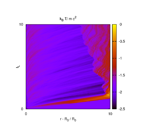
Figure 4.— The time evolution of the temperature profile $k_{B}T/mc^{2}$ in the case of $R_{\mathrm{top}}=11R_{0}$. The horizontal axis is the radius $(r-R_{0})/R_{0}$, and the vertical axis is time measured in the light crossing time $t_{L}\equiv 10t_{0}$. The left-hand edge is the neutron star surface and the right-hand edge is the top of the flux tube. The red region emerging at the origin is the region between the front edge of the Alfvén waves and the initially generated slow shock front.

Figure 4 is the time evolution of temperature profile. The red belt in the lower region of this figure is a hot region heated by the Alfvén waves. The lower boundary of this region corresponds to the front edge of Alfvén waves and the upper boundary to the slow shock front generated on the neutron star surface at the initial time. This figure shows that the highest temperature resulted from the collision of the hot regions at the loop top. This temperature rising continues until the arriving of the slow shock, and afterwards this region gradually expands absorbing the subsequent Alfvén waves.

As is well known, waves have their own energy and momentum flux and can produce an extra pressure called ’wave pressure’ whose typical form is given by $P_{w}=\rho h\langle\delta v^{2}\rangle/2$. Following the traditional wave driven wind theory (Lamers & Cassinelli, 1999), as waves propagate outwards in stellar atmospheres with decreasing density, the wave pressure gradient is generally generated. This wave pressure gradient induces a force on the background plasma and this results in a transonic outgoing flow called ’wave driven wind’. Differently from the ordinary wave driven wind cases, we impose the reflection boundary at the loop top, so that the radial velocity is not transonic. The radial velocity profile, however, shows that the Alfvén waves produce the wave-pressure and drive upgoing flows. Note that these upgoing flows play an essential role in the mass supply to the loop top regions, which triggers giant flare-like phenomena as discussed below.

In addition to the Alfvén waves, we find that a slow shock induced by the initial high-temperature atmosphere plays a very important role for the evolution of the magnetosphere. Because of the initial pressure gradient between the atmosphere and the magnetosphere plasma, a slow shock is generated just after starting the calculation. This slow shock propagates outwards approximately about the relativistic sound velocity $c_{s,r}\equiv c/\sqrt{3}$, and heats the plasma (The slow shock is at $r-R_{0}\sim 0.6,7$ when $t=0.2t_{L},t_{L}$ in Figure 3). When this slow shock reaches the loop top, the background plasma is heated drastically by the collision of two slow shocks, which results in the initial spike of flares as is explained later; the plasma temperature around the loop top becomes more than $0.1mc^{2}$. After the shock reaches the loop top, the plasma reaches a quasi-steady state and the plasma continues to be heated slowly by slow shocks generated by Alfvén waves .

3.2. Temperature Evolution at the Loop Top

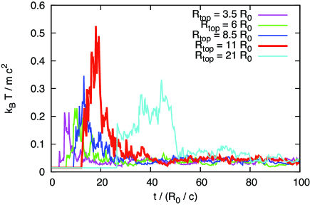
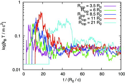
Figure 5.— The temporal evolution of the temperature $k_{B}T/mc^{2}$ at the loop top: $R_{\mathrm{top}}=3.5,6,8.5,11,21R_{0}$. We assumed $\langle\delta v_{\perp}\rangle=0.75c_{s,r}$. Top: normal-scale. Bottom: log-scale

In this paper, we assumed the existence of the initial high temperature atmosphere resulting from some burst phenomena. As explained in the previous section, this structure induces a strong slow shock and this slow shock heats plasma in the magnetosphere. In this section, we focus on the evolution of the temperature at the loop top and study its implication in the giant flare. Here we assume the existence of a mechanism triggering the giant flare and we do not discuss its origin.

Figure 5 is the temporal evolution of the loop top temperature using various loop size: $R_{\mathrm{top}}=3.5,6,8.5,11,21R_{0}$. First we note that the temperature keeps its initial value until $t\sim(R_{\mathrm{top}}-R_{0})/c_{A}$, or the Alfvén crossing time along the loop. Around $t=(R_{\mathrm{top}}-R_{0})/c_{A}$, the Alfvén waves emitted at initial time reach the loop top and collides with waves that propagate from the other side of the loop as indicated in Figure 4. Note that the Alfvén waves are accompanied by hot plasma regions resulted from the shock heating and the Alfvén waves’ dissipation as shown in Appendix B, the compression by the collision of this region induces the initial temperature rise. The temperature reaches its maximum value of about $0.3k_{B}T/mc^{2}$ at $t\sim(R_{\mathrm{top}}-R_{0})/c_{\textrm{slow}}$ where $c_{\textrm{slow}}\sim c_{s,r}\equiv c/\sqrt{3}$ is the slow shock velocity observed in our simulation, which is equivalent to the time when the slow shock induced by the initial pressure discontinuity at the atmosphere reaches the loop top. Afterwards, the temperature shows quasi-stable behavior with small perturbations by the Alfvén waves.

This panel shows that the maximum temperature increases with loop size until $R_{\mathrm{top}}=11R_{0}$; in the case of $R_{\mathrm{top}}=21R_{0}$, the maximum temperature is smaller than that of $R_{\mathrm{top}}=11R_{0}$, but the duration of the temperature rising becomes longer. This can be explained as follows.

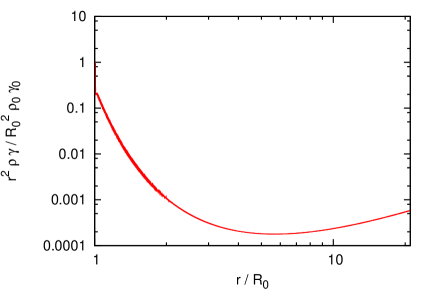
Figure 6.— A snapshot of the initial mass profile in the spherical shell per unit radial coordinate.

Assuming the initially triggered slow shock as a blast wave, the conservation law of the wave energy flux can be written as, $\rho(\delta v)^{2}c_{s}f(r)\sim\mathrm{Const.}$, when background velocity is sufficiently smaller than background sound velocity (Lamers & Cassinelli, 1999). Thus, the temperature of the blast wave is

$$\delta T\sim(\delta v)^{2}\propto(\rho f(r)c_{s})^{-1}.$$ (8)

Note that now the wave group velocity $c_{s}$ takes a constant value, $c/\sqrt{3}$, so that the temperature of the slow shock region is in proportion to $(\rho f(r))^{-1}$. Figure 6 is the initial profile of the mass in the spherical shell per unit radial coordinate, $\rho f(r)$, using an approximation: $f(r)\sim r^{2}$. It shows that the mass profile has a minimum point around $r\sim 6R_{0}$. Equation (8) indicates that the temperature at the loop top increases with increasing the length of the loop until it reaches the above minimum point, and this explains the tendency of our numerical results very well. Figure 6 shows that the radial gradient of the mass around the minimum point is not so steep, and we consider that this is the reason why the shock strength still increases beyond the minimum point as shown in the bottom panel of Figure 5. Note that Equation (8) can also be applied to the Alfvén waves, so that heating by Alfvén waves does not change the above argument essentially.

The above radial coordinate at the minimum mass point can be obtained as follows. First, if we assume the non-relativistic hydrostatic equilibrium, the mass profile can be written as: $\rho=\rho_{0}\exp[-\frac{r-R_{0}}{H}\frac{R_{0}}{r}]$ where $H=(R_{0}/r_{g})(c_{s}/c)^{2}R_{0}$ is the scale height, $\rho_{0}$ is the density at $r=R_{0}$ and $c_{s}$ is the sound velocity. Using this expression, the minimum point can be calculated as:

$$\frac{d}{dr}[r^{2}\rho]\propto 2\rho\left[r-\frac{R_{0}^{2}}{2H}\right].$$ (9)

From this equation, we can obtain the radial coordinate of the minimum mass point as

$$r_{\mathrm{min}}/R_{0} = R_{0}/2H$$ (10)

$$\sim 8\left(\frac{r_{g}}{0.3R_{0}}\right)\left(\frac{c_{s}(T=7.5\textrm{[keV]})}{c}\right)^{-2}.$$

The minimum value in Figure 6 seems a little smaller than this value because of the general relativistic effect. This coordinate is a critical value at which the strength of the shocks change, so that this can be used as a characteristic coordinate of this phenomena.

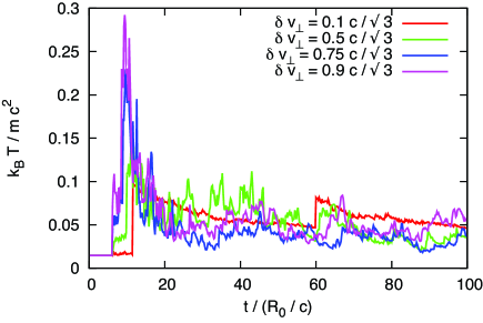
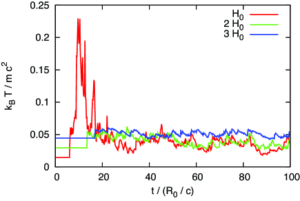
Figure 7.— The temporal evolution of the temperature $k_{B}T/mc^{2}$ at the loop top $R_{\mathrm{top}}=6R_{0}$. Top: amplitude dependence. Bottom: scale height dependence. $H_{0}$ is the scale height in the case of $T=7.5$ [keV].

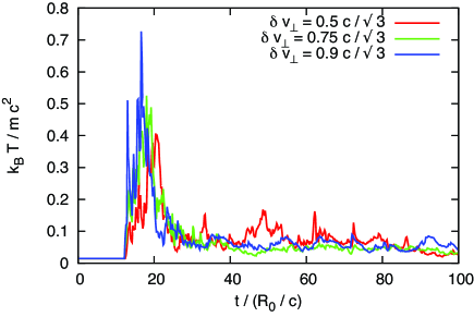
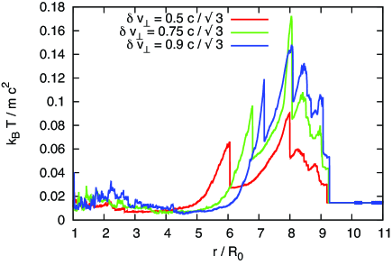
Figure 8.— Top: The temporal evolution of the temperature $k_{B}T/mc^{2}$ at the loop top $R_{\mathrm{top}}=11R_{0}$ using different wave amplitude. Bottom: Snapshots of the temperature profile at $t=10R_{0}/c$.

Next, we discuss their dependence on the amplitude of the Alfvén waves and scale height $H=(R_{0}/r_{g})(c_{s}/c)^{2}R_{0}$. The top panel of the Figure 7 is the temporal evolution of the loop top temperature whose length is $R_{\mathrm{top}}=6R_{0}$ using different Alfvén wave amplitude. This figure shows the peak temperature increases with increasing the wave amplitude. This is because more energy is supplied to the hot region heated by the Alfvén waves as the amplitude of the waves increases. This also reduces the energy loss of the shock waves propagating through the cold plasma, and help to keep the strong shock condition. On the other hand, when $\langle\delta v_{\perp}\rangle/c_{s,r}=0.1$, the contribution from the Alfvén waves is significantly decreased, so that there is no initial spike like feature in their curve but steep temperature rising by the collision of the slow shocks that is driven by the initial pressure gradient at the atmosphere. Note that the rising time of the initial spike is moved forward as the wave amplitude increases. This can be explained by the same reason because the shock front velocity becomes faster as the temperature in a post-shock region increases. Concerning the amplitude, the amplitudes used in our simulations are too large comparing with a theoretical value, $\delta v_{\perp}\sim 0.01c$, predicted by Blaes et al. (1989). However, even if the predicted amplitude is used, our mechanism works in the magnetar magnetosphere because of its Poynting-dominated environment where even Alfvén waves with small amplitude have much larger energy than background thermal energy; on the other hand, our simulations considered a plasma with moderate magnetization, $\sigma\leq 10$, so that the larger wave amplitude is necessary to produce a sufficient energy on the background plasma. The detailed estimate of their energetics is discussed in Section 4.3. In the bottom panel of the Figure 7, we plot the temporal evolution of the loop top temperature using different values of $r_{g}/R_{0}$ to study the scale height dependence. We find the peak energy decreases with increasing the scale height. This is because both the density and pressure in front of the shock fronts increase with increasing the scale height, and we cannot neglect the pressure in the magnetosphere comparing with the pressure in the postshock region, which means the breakdown of the strong shock condition.

Top panel of Figure 8 is the temporal evolution of the temperature at the loop top whose length is $R_{\mathrm{top}}=11R_{0}$. This panel shows that, compared with the case of $R_{\mathrm{top}}=6R_{0}$, their maximum temperature shows similar dependence on the wave amplitude, though the amount of their difference becomes small. Bottom panel of Figure 8 is a snapshot of the temperature profile of each wave amplitude cases just before their collision with their counter parts from the other side of loop. At $r\sim 9.2R_{0}$, there are fast shock fronts induced by the collapse of the Alfvén waves. Since the fast velocity is close to the light velocity in high-$\sigma$ plasmas, the fronts of the 3 cases are at the same position. On the other hand, the position of slow shock fronts, located around $r=6-7R_{0}$ in the figure, depends on their amplitude; their coordinate increases with increasing the Alfvén wave amplitude because of the energy supply to the slow shocks from the Alfvén waves. Note that in the top panel of Figure 8, all the initial temperature rising occur at the same time. However, the time of their peak temperature are delayed as the wave amplitude decreases. We consider that this also supports our conclusion that the initial temperature rising is caused by the hot region heated by the Alfvén waves and the peak temperature is controlled by the collision of the initially induced slow shocks at the atmosphere.

4. Discussion

4.1. Light Curves

In Section 3.2, we showed the temperature evolution at the loop top. In this section, we discuss the possibility of the relation between the initial spike of giant flares and the collision of shocks at the loop top. We note that the curves in the bottom panel of Figure 5 are similar to the light curve of flare phenomena. In addition, the maximum temperature of the curves reaches $100$ [keV]. These indicate that the collision of shocks at loop tops can be a candidate of the mechanism of the initial spike of magnetar giant flares. To examine this, we consider the time scale of this phenomena in the case of magnetar. Using $R_{0}\sim 10^{6}$[cm] and $c=3\times 10^{10}$[cm/s], the light crossing time of the central star becomes $t_{0}=R_{0}/c\sim 0.03$ [ms]. From the above discussion, the duration of the temperature rising, which corresponds to the time lag of the arrivals of the Alfvén waves and the slow shock, can be estimated as

$$\Delta t\sim r_{\mathrm{min}}/c_{\mathrm{slow}}-r_{\mathrm{min}}/c_{A}.$$ (11)

Using the following parameters: $r_{\mathrm{min}}=8R_{0},c_{A}=c,c_{\mathrm{slow}}=c_{s,r}$, the duration becomes $\Delta t\sim 0.3$ [ms]. The observed rising time of the initial peak of the giant flare is $\sim 1$ [ms], so the obtained value in our simulation is of the same order. Note that this conclusion is obtained using flux tubes with length $R_{\mathrm{top}}>r_{\mathrm{min}}$; if we take into account shorter flux tubes, the total duration time, which is the superposition of the flares of tubes with various length, can be longer, since initial rising time of shorter tubes is earlier than that of longer tubes.

Concerning the average temperature during the collision of heated regions, we can estimate its value as follows. First, the slow shock initially driven by the star surface is a strong shock propagating into the cold magnetosphere along the radially-expanding closed loop. This can be approximated by the non-relativistic strong shock. The temperature just inside of slow shocks can be written as:

$$k_{B}T/mc^{2}=2\frac{\Gamma-1}{(\Gamma+1)^{2}}\left(\frac{u_{\textrm{sh}}}{c}\right)^{2}\simeq 0.04\left(\frac{u_{\textrm{sh}}}{c_{s,r}}\right)^{2},$$ (12)

where we used $\Gamma=4/3$ and $u_{\textrm{sh}}$ is the shock velocity in the upstream comoving frame. Here we used the observed value $c_{s,r}$ . Note that this value approximately reproduces the result in Figure 3 (see around $r=5-6R_{0}$ of the blue line in the left-bottom panel). Next, the collision of the above region heated by the Alfvén waves results in two slow shock fronts due to their supersonic velocity and the post-shock region behind the shock fronts is equivalent to the temperature rising state in Figure 5. Since the nature of the slow shock in high-$\sigma$ plasmas is close to hydrodynamic shocks, we derive the post-shock temperature using the results of the pure hydrodynamic Riemann problem  (Marti & Muller, 1994; Mignone et al., 2005). Following the relativistic Rankine-Hugoniot relation, the post-shock pressure can be written as follow:

$$p_{ps} = p_{u}+\frac{h_{ps}\gamma_{ps}v_{ps}-h_{u}\gamma_{u}v_{u}}{\zeta},$$ (13)

$$\frac{1}{\rho_{ps}\gamma_{ps}} = \frac{1}{\rho_{u}\gamma_{u}}-\zeta(v_{ps}-v_{u}),$$ (14)

where subscript “u” and “ps” means the variables are in upstream region and post-shock region, respectively, and

$$\zeta=\frac{1}{\rho_{u}\gamma_{u}(v_{sh}-v_{u})}.$$ (15)

In the above expression, $v_{sh}$ is the velocity of the shock front. Since the heated region collides with the counter part propagating from the other side of the loop, the flow velocity in the post-shock region is $v_{ps}=0$ due to the conservation of momentum. For simplicity, we assume the shock front velocity $v_{sh}=-c_{s,r}$ . In this case, using the above equations, we can obtain the following expression of the post-shock temperature:

$$\frac{k_{B}T_{ps}}{mc^{2}}=\frac{p_{ps}}{\rho_{ps}}=\frac{p_{u}}{\rho_{u}\gamma_{u}}\left[1-\frac{v_{u}}{c_{s,r}+v_{u}}\right]+c_{s,r}h_{u}\gamma_{u}v_{u}.$$ (16)

By substituting $T_{u}=0.04mc^{2}$, obtained in Equation (12), and $v_{u}=2v_{sh}/(\Gamma+1)$ that is the post-shock velocity in the case of strong shocks, we obtain $T_{ps}\sim 0.4mc^{2}$ that reproduces the average value of the top panel of Figure 5 well. Although this value is much smaller than that in the case of $R_{\mathrm{top}}=11R_{0}$, we consider this is due to the dynamical effect by the Alfvén waves. Note that the above value does not depend on the detailed state of the plasma, especially independent of the temperature on the star surface and in the magnetosphere. This is due to using the strong shock solution and the Rankine-Hugoniot relation, so that the above temperature can be obtained as long as we prepare conditions which are natural in the case of magnetar giant flares and can results in the initial strong shocks. As we will comment later, if we increase the temperature in the magnetosphere, the above strong shock condition is broken and the resulted maximum temperature decreases.

Thompson & Duncan (1995) showed that in the fireball region caused by a SGR flare phenomena the total Thomson optical depth across a scale of the neutron star radius $R_{0}\sim 10^{6}$ [cm] becomes optically thick: $\tau_{T}\sim 5\times 10^{7}\gg 1$. The above estimate uses the typical values of the SGR flares, so the optical depth becomes also much larger than unity in the case of the magnetar giant flare. This means that the photons trapped in the fireball region cannot escape and cannot be observed. Our flare mechanism always works at the top of the magnetic loop, so that the generated photons can escape from the fireball region. In addition, because of the very short mean free path of the scattering between photons and pairs, the photon temperature takes the same value of the pair plasma. Hence, the observed photon temperature behaves as Figure 5. As shown in Section 3.2, the strength of the initially triggered slow shock gradually decreases after it reaches $r_{\mathrm{min}}$ given in Equation (10). Then, the spike form of the light curve gradually disappear during $\sim$ ms time scale, and at a later time we will observe the temperature on the surface of the fireball, as is indicated by observations (Woods & Thompson, 2006; Mereghetti, 2008).

In this paper, we assumed the mirror symmetry of flux tubes. This may be a too idealized situation for real magnetar giant flare, and imbalanced collision of the two slow shocks may be more realistic. However, as is discussed in Section 3.2, the shocks become sufficiently strong if the flux tube length is longer than the critical length. Hence, we expect that even imbalanced collisions can produce sufficient energy as long as the collision occurred further than the critical length.

Finally, we give a comment on a possibility of our shock collision mechanism playing an important role even in the twisted magnetic flux rope model. The collisionless magnetic reconnection converts the upstream magnetic field energy mainly into the plasma kinetic energy due to the collisionless nature, not in the thermal energy, so that another energy conversion mechanism is necessary for explaining the light curve of the giant flares in magnetars. We expect that our mechanism can give an explanation of the energy conversion from the kinetic energy into the thermal energy.

4.2. Properties of Closed Flux Tubes

In this paper, we used 1-dimensional approximation and introduced the closed flux tube that super-radially expands, given by Equation (1). In this section, we discuss properties of the flux tube in magnetars. Detailed dependence of numerical results on the configuration of the radially-expanding closed loop is given in Appendix C.

This flux tube expands super-radially at the bottom. In the case of the Sun, this structure is considered to result from the rapid decrease of the gas pressure on the surface  (Shibata & Uchida, 1986; Tian et al., 2010). Inside of the Sun, there is a lot of hot matter, and the gas pressure dominates the magnetic pressure, so that the flux tube of the magnetic field cannot expand. However, as leaving from the surface, the amount of matter and the gas pressure rapidly decrease and this allows the super-radial expansion of the flux tube due to its strong magnetic pressure.

As indicated in Equation (2), the flux tube results in the split monopole like magnetic field $B\propto 1/r^{2}$ instead of the dipole field $B\propto 1/r^{3}$. In case of the Sun, the monopole like magnetic field results from the dragging of magnetic field line by the matter on the line. On the other hand, the above mechanism does not seem to work on the magnetic field close to the magnetar surface because of the very strong magnetic field. However, in case of the giant flare, the observed isotropic peak luminosity of initial spike reaches $F_{\mathrm{SGR}}\sim 10^{46}$ [erg/s] (Terasawa et al., 2005; Hurley et al., 2005; Tanaka et al., 2007), so that the energy density of the fireball region can be estimated as:

$$e_{\mathrm{Spike}} \sim F_{\mathrm{Spike}}\Delta t/4\pi R^{2}\Delta R$$ (17)

$$\sim 10^{24}\left(\frac{\Delta t}{1[\textrm{ms}]}\right)\left(\frac{R}{10^{6}[\textrm{cm}]}\right)^{-2}$$

$$\times \left(\frac{\Delta R}{10^{6}[\textrm{cm}]}\right)^{-1}[\textrm{erg/cm${}^{3}$}],$$

where $\Delta t$ is the duration of the initial spike, $\Delta R$ is the radius of the fireball region. The magnetic field energy density can be written as:

$$e_{B}=B^{2}/8\pi\sim 10^{26}\left(\frac{B_{0}}{10^{14}[\textrm{G}]}\right)^{2}\left(\frac{R}{10^{6}[\textrm{cm}]}\right)^{-6}[\textrm{erg/cm${}^{3}$}],$$ (18)

where $B_{0}$ is the magnetic field strength on the magnetar surface. Comparing Equations (17) and (18), the fireball energy density can exceed the magnetic field energy when the fireball region expands sufficiently. Thus, we expect that the magnetic field can be dragged by the matter energy in the fireball region as the fireball evolves, and finally induces spherically expanding flux tube structure   . Observationally, detection of large flux changes in the persistent X-ray flux of magnetars have been reported during giant flares (Woods et al., 2001), and this is thought to be an indication of the change of the global magnetic field structure in magnetar magnetospheres. We consider that this is an evidence for occurring a similar phenomena reported in solar atmosphere, e.g. (Shibata & Uchida, 1986; Tian et al., 2010), which is also an change of magnetic field structure during solar flares, inducing super-radially expanding flux tubes. Although this indicates the highly dynamical flux tubes, we expect that the quasi-steady assumption of the flux tube is still not so bad approximation since the timescale of the evolution of flux tubes is thought to be comparable to that of tearing instability, which is longer than the characteristic timescale of our model, that is, the Alfvén crossing time. Note that even if the actual magnetic field is not the super-radial flux tube but the dipole, our flare mechanism can still be applicable since our mechanism does not depend strongly on the magnetic field structure as explained in Section 3.2. In particular, even if we consider a flux tube with $f(r)\propto r^{n}$, the characteristic length-scale $r_{\mathrm{min}}$ given by Equation (10) becomes just $R_{0}^{2}/nH$, and the characteristic timescale Equation (11) is nearly independent of the background magnetic field with low multi-pole components. Note that this argument can generally be used if the background plasma density is determined by the gravity of the central star.

Concerning another models of plasma density in magnetar magnetospheres, Thompson & Duncan (1995) estimated the plasma density in the fireball region in the case of $B\gg B_{\mathrm{QED}}$ and $k_{B}T\ll m_{e}c^{2}$ which is given as follows

$$n^{\pm}=\frac{(m_{e}c)^{3}}{\hbar(2\pi^{3})^{1/2}}\left(\frac{B}{B_{\mathrm{QED}}}\right)\left(\frac{k_{B}T}{m_{e}c^{2}}\right)\exp\left[-\frac{m_{e}c^{2}}{k_{B}T}\right],$$ (19)

where $B_{\mathrm{QED}}=m_{e}^{2}c^{3}/e\hbar=4.4\times 10^{13}$[G] is the magnetic field strength at which the quantum effect starts to work. In the paper, they did not take into account the effect of the gravity. In addition, Thompson et al. (2002) derived another form of the mass density in the case of the magnetosphere with toroidal magnetic field. To determine which model of the plasma density is the correct one is beyond the scope of our paper, and we would like to consider it for our future work.

4.3. Effects of Alfvén waves and $\sigma$-Parameter

In this paper, we assume the continuous injection of Alfvén waves driven on the star surface. We found that the injected Alfvén waves transfer matter and energy through their propagation and dissipation, and they also play a key role to the flare phenomena through heating the initially driven slow shock by their dissipation. The Alfvén wave energy density can be written as follows:

$$e_{\mathrm{A,wave}}=(\delta B)^{2}/8\pi=(1/\sigma+1)(\delta v_{\perp}/c)^{2}e_{B},$$ (20)

where $e_{B}=B^{2}/8\pi$ is the background magnetic field energy density and we used Equation (B1) and $\sigma=B^{2}/4\pi\rho h$. The energy flux of Alfvén waves can be written as:

$$F_{\mathrm{A,wave}} = e_{\mathrm{A,wave}}R^{2}v_{A}$$ (21)

$$\sim 10^{45}\left(\frac{\delta v_{\perp}/c}{10^{8}\mathrm{[cm/s]}/c}\right)^{2}\left(\frac{c_{A}}{3\times 10^{10}[\textrm{cm/s}]}\right)$$

$$\left(\frac{B_{0}}{10^{14}[\textrm{G}]}\right)^{2}\left(\frac{R}{10^{6}[\textrm{cm}]}\right)^{2}[\textrm{erg/s}].$$

where $\delta v_{\perp}=10^{8}$[cm/s] is a typical shear wave velocity in crusts obtained by Blaes et al. (1989). Equation (21) indicates that the amplitude used in our simulations, $\langle\delta v_{\perp}\rangle=0.75c_{s,r}$, is too large to explain the observation. However, as discussed in Section 3.2, the most important effect of the Alfvén waves is to supply energy to the initially triggered slow shock and keep its behavior to satisfy the strong shock condition. If we assume that a fraction $\epsilon$ of the Alfvén wave energy density dissipate into thermal energy, the resulted temperature can be expressed as $k_{B}T/mc^{2}=\epsilon e_{\mathrm{A,wave}}/\rho c^{2}\sim\epsilon\sigma(\delta v_{\perp}/c)^{2}$. Using typical parameters for magnetars, $\langle\delta v_{\perp}\rangle/c\sim 10^{-2}$ (Blaes et al., 1989) and $\sigma\sim 10^{4}$ (see also the footnote ) , even small dissipation, such as $\epsilon\sim 10^{-2}$, is sufficient for resulting in heating the magnetosphere more than $50$ [keV], which is enough to keep the strength of the slow shock. In Appendix B, we also provide a study of behaviors of Alfvén waves in Poynting-dominated plasma with $\sigma$ value from $1$ to $500$. The results show that though the dissipation rate becomes smaller as the $\sigma$ parameter increases, the resulting temperatures are almost independent of the $\sigma$ parameter due to the increase of the magnetic field energy comparing with the thermal energy of the background plasma. This indicates that the increase of $\sigma$ parameter in a magnetar magnetosphere makes our flare mechanism easier to work.

In this paper, we also assumed the MHD approximation in the magnetar magnetosphere. If some burst phenomena occur and result in a fireball, the number density of the electron positron pair increases drastically. In addition, the rapid interaction between photons and pairs allows the particle distribution to be an equilibrium state. Hence, we expect that at least in the fireball region we can use MHD approximation and Alfvén waves can propagate. Concerning the dissipation of the Alfvén waves, we considered the dissipation through the shock forming by the non-linear effect of waves. However, there are other possibilities. For example, the wave decay process can play an important role since the particle number density is small in the vicinity of the shock front of the initially triggered slow shock. Recently, it was proved that the wave decay processes can dissipate Poynting energy in a back ground plasma very efficiently (Amano & Kirk, 2013; Mochol & Kirk, 2013a, b). Since the main role of Alfvén waves in our mechanism is the heating of the slow shock, this means that the plasma effects on the decay of the Alfvén waves do not change our physical picture but even encourages to work.

Appendix A Numerical Method

In this appendix, we present the detailed explanation of the numerical method we use in this paper. Variables indicated by Greek letters take values from $0$ to $3$, and those indicated by Roman letters take values from $1$ to $3$.

As is mentioned in Sec. 2.2, we solve the dynamical evolution of the plasma and waves by solving the ideal GRMHD equations in Schwarzschild spacetime whose

$$ds^{2} = g_{\mu\nu}dx^{\mu}dx^{\nu},$$

$$= -w(r)dt^{2}+w(r)^{-1}dr^{2}+r^{2}(d\theta^{2}+\sin^{2}\theta d\phi^{2}),$$

where $w(r)=1-r_{g}/r$, $r_{g}\equiv 2MG/c^{2}$ is the Schwarzschild radius, $M,G,c$ are the central star mass, the gravitational constant and the light velocity, respectively. We use the metric signature, $(-,+,+,+)$, along with units $c=1$.

The basic equations are the mass conservation, the energy-momentum conservation and the induction equation which are given as:

$$\nabla_{\mu}N^{\mu} = \frac{1}{\sqrt{-g}}\partial_{\mu}[\sqrt{-g}N^{\mu}]=0,$$ (A2)

$$\nabla_{\mu}T^{\mu}_{\nu} = \frac{1}{\sqrt{-g}}\partial_{\mu}[\sqrt{-g}T^{\mu}_{\nu}]-\frac{1}{2}g_{\mu\rho,\nu}T^{\mu\rho}=0,$$ (A3)

$$\nabla_{\mu}(^{*}F^{\mu\nu}) = \frac{1}{\sqrt{-g}}\partial_{\mu}[\sqrt{-g}(^{*}F^{\mu\nu})]=0,$$ (A4)

where $N^{\mu}\equiv\rho u^{\mu}$ is the mass flux vector, $\rho$ is the mass density in the fluid comoving frame, $u^{\mu}$ is the 4-velocity which satisfies $u^{\mu}u_{\mu}=-1$; $T^{\mu\nu}$ is the energy-momentum tensor defined as

$$T^{\mu\nu}=(\rho h+|b|^{2})u^{\mu}u^{\nu}+(p_{\mathrm{gas}}+|b^{2}|/2)g^{\mu\nu}-b^{\mu}b^{\nu},$$ (A5)

where $h$ is the specific enthalpy, $p$ is the gas pressure, $b^{\mu}=(g_{i\mu}B^{i}u^{\mu},(B^{i}+u^{i}b^{t})/u^{t})$ is the magnetic field 4-vector, $B^{i}$ is the magnetic field in the laboratory frame; ${}^{*}F^{\mu\nu}$ is the dual of the electromagnetic field strength tensor given by ${}^{*}F^{\mu\nu}=u^{\mu}b^{\nu}-u^{\nu}b^{\mu}$.

To use the HLLD approximation, we introduce the following 4-vector $\tilde{u}^{\mu}=(\tilde{\gamma},\tilde{\gamma}\tilde{{\bf v}})$

$$\tilde{u}^{\mu}\equiv(\sqrt{w}u^{t},u^{r}/\sqrt{w},ru^{\theta},r\sin\theta u^{\phi}).$$ (A6)

Using this 4-vector, the square of the 4-velocity $u^{\mu}$ can be expressed as: $u_{\mu}u^{\mu}=-(\tilde{u}^{t})^{2}+(\tilde{u}^{r})^{2}+(\tilde{u}^{\theta})^{2}+(\tilde{u}^{\phi})^{2}=\eta_{\mu\nu}\tilde{u}^{\mu}\tilde{u}^{\nu}=-1$ where $\eta_{\mu\nu}=\mathrm{diag}(-1,1,1,1)$. In addition, we also introduce the following 3-vector $\tilde{B}^{i}$

$$\tilde{B}^{i}=(B^{r},\sqrt{w}rB^{\theta},\sqrt{w}r\sin\theta B^{\phi}).$$ (A7)

Using this 3-vector, the 4-magnetic field vector $b^{\mu}$ can be expressed as follows:

$$b^{\mu}=(\tilde{b}^{t}/\sqrt{w},\sqrt{w}\tilde{b}^{r},\tilde{b}^{\theta}/r,\tilde{b}^{\phi}/r\sin\theta)$$ (A8)

where $\tilde{b}^{\mu}$ is defined as:

$$\tilde{b}^{\mu}=(\tilde{\gamma}(\tilde{{\bf B}}\cdot\tilde{{\bf v}}),\quad\tilde{{\bf B}}/\tilde{\gamma}+\tilde{\gamma}(\tilde{{\bf B}}\cdot\tilde{{\bf v}})\tilde{{\bf v}}),$$ (A9)

where $\tilde{{\bf B}}\cdot\tilde{{\bf v}}=\tilde{B}^{r}\tilde{v}^{r}+\tilde{B}^{\theta}\tilde{v}^{\theta}+\tilde{B}^{\phi}\tilde{v}^{\phi}$. Similarly to $\tilde{u}^{\mu}$, the square of the 4-magnetic field vector can be rewritten as: $b_{\mu}b^{\mu}=\eta_{\mu\nu}\tilde{b}^{\mu}\tilde{b}^{\nu}$.

Using these new vectors, the basic equations Equations (A2), (A3), (A4) can be rewritten as

$$\partial_{t}U+\partial_{r}F^{r}+S=0,$$ (A10)

$$\tilde{B}^{r}\sqrt{-g}=\mathrm{const.},$$ (A11)

where

$$U=\left(\begin{array}[]{ccc}\sqrt{-g/w}&\times&\rho\tilde{\gamma}\\ \sqrt{-g}/w&\times&[(\rho h+\tilde{b}^{2})\tilde{\gamma}^{2}\tilde{v}^{r}-\tilde{b}^{t}\tilde{b}^{r}]\\ r\sqrt{-g}/\sqrt{w}&\times&[(\rho h+\tilde{b}^{2})\tilde{\gamma}^{2}\tilde{v}^{\perp}-\tilde{b}^{t}\tilde{b}^{\perp}]\\ \sqrt{-g}&\times&[(\rho h+\tilde{b}^{2})\tilde{\gamma}^{2}-(p_{\mathrm{gas}}+\tilde{b}^{2}/2)-(\tilde{b}^{t})^{2}]\\ \sqrt{-g/w}/r&\times&\tilde{B}^{\perp}\end{array}\right),$$ (A17)

$$F^{r}=\left(\begin{array}[]{ccc}\sqrt{-gw}&\times&\rho\tilde{\gamma}\tilde{v}^{r}\\ \sqrt{-g}&\times&[(\rho h+\tilde{b}^{2})\tilde{\gamma}^{2}(\tilde{v}^{r})^{2}+(p_{\mathrm{gas}}+\tilde{b}^{2}/2)-(\tilde{b}^{r})^{2}]\\ r\sqrt{-gw}&\times&[(\rho h+\tilde{b}^{2})\tilde{\gamma}^{2}\tilde{v}^{r}\tilde{v}^{\perp}-\tilde{b}^{r}\tilde{b}^{\perp}]\\ w\sqrt{-g}&\times&[(\rho h+\tilde{b}^{2})\tilde{\gamma}^{2}\tilde{v}^{r}-\tilde{b}^{t}\tilde{b}^{r}]\\ \sqrt{-gw}/r&\times&[\tilde{B}^{\perp}\tilde{v}^{r}-\tilde{B}^{r}\tilde{v}^{\perp}]\end{array}\right),$$ (A23)

$$S=\left(\begin{array}[]{c}0\\ -\frac{\sqrt{-g}}{2}\left[\frac{(r^{2})^{\prime}}{r^{2}}\left\{(\rho h+\tilde{b}^{2})(\tilde{u}^{\perp})^{2}+2(p_{\mathrm{gas}}+\tilde{b}^{2}/2)-(\tilde{b}^{\perp})^{2}\right\}\right.\\ -\left.\frac{w^{\prime}}{w}\left\{(\rho h+\tilde{b}^{2})[\tilde{\gamma}^{2}+(\tilde{u}^{r})^{2}]-(\tilde{b}^{t})^{2}-(\tilde{b}^{r})^{2}\right\}\right]\\ 0\\ 0\\ 0\end{array}\right),$$ (A30)

where $\perp=\theta,\phi$. Note that the conservative variables $U$ and the numerical flux $F^{r}$ have a form $\alpha_{\mathrm{curv}}U_{\mathrm{RMHD}}$ and $\beta_{\mathrm{curv}}F_{\mathrm{RMHD}}$ where $U_{\mathrm{RMHD}}$ and $F_{\mathrm{RMHD}}$ are the conservative variables and the numerical flux of the relativistic MHD equations in the flat geometry, $\alpha_{\mathrm{curv}}$ and $\beta_{\mathrm{curv}}$ are curvature terms. We calculate numerical flux $F^{r}$ as the following form, $F^{r}=\beta_{\mathrm{curv}}F_{\mathrm{HLLD}}$, where $F_{\mathrm{HLLD}}$ is the HLLD flux calculated using $U_{\mathrm{RMHD}}$ and $F_{\mathrm{RMHD}}$. In this case, the HLLD flux is not a good approximation comparing with the flat geometry case. However, it is a better estimation for the numerical flux, especially when $\Delta r/r\ll 1$ where $\Delta r$ is the mesh size. Concerning the term $S$, we calculate it as a source term at $t=t^{n}+\Delta t/2$ where $t_{n}$ is the time at n-th time steps and $\Delta t$ is the size of a time step. To calculate the primitive variables from the conservative variables, we used a method developed by Mignone & McKinney (2007) which allows us to calculate the primitive valuables very accurately. (see also (Beckwith & Stone, 2011)) Note that we calculate along flux tube with super-radial expansion structure, so that the radial coordinate $r$ accompanying with the angular components $(\theta,\phi)$ of the above tensors should be changed into $r\sqrt{f}$ where $f$ is defined in Equation (1), for example, $\sqrt{-g}\equiv r^{2}f\sin\theta$.

Appendix B Propagation of Alfvén Waves in Poynting-Dominated Plasmas

In this section, we investigate the $\sigma$-dependence of an evolution of the linearly polarized Alfvén waves with large amplitude. Differently from the circularly polarized case, the linearly polarized Alfvén wave with large amplitude is not an exact solution of RMHD equations. Hence, immediately after their generation, e.g. by an oscillation of a neutron star surface, they change the background plasma structure by their magnetic pressure force and it induces their effective dissipation.

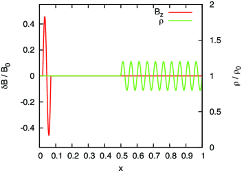
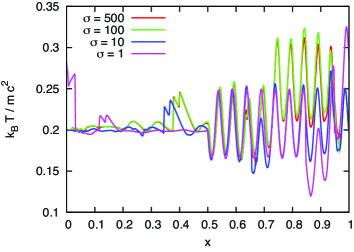
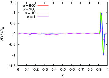
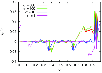
Figure 9.— Snapshots of the propagation of an Alfvén wave. Left top: initial snapshots of the density and magnetic field. Left bottom: snapshot of the magnetic field in the unit of the initial amplitude at $0.9$ Alfvén crossing time. Right top: snapshot of the temperature at $0.9$ Alfvén crossing time. Right bottom: snapshot of the velocity $v_{x}$ at $0.9$ Alfvén crossing time.

In this calculation, we prepared a numerical domain: $0<x<1$, and divided it using uniform meshes with size $\Delta x=2.5\times 10^{-4}$. The background temperature is $p_{0}/\rho_{0}=0.2$ where subscript $0$ means the variables are averaged values. We used the ideal equation of state $h=1+\Gamma/(\Gamma-1)p/\rho$ with $\Gamma=5/3$. For the Alfvén wave, we prepared a linearly polarized Alfvén wave with amplitude $\delta B=B_{0}/2$ whose wavelength is $0.05$ times of the length of the numerical domain. To simulate disturbances from the density decrease in the magnetar magnetosphere, we set sinusoidal density disturbance with amplitude $0.2\rho_{0}$ as in the left-top panel of Figure 9. We used the periodic boundary condition. For the initial condition of an Alfvén wave, we consider

$$B^{z}=\delta B\sin(2\pi x/\lambda),\quad v^{z}=-\frac{B^{z}}{\sqrt{4\pi\rho h+|B|^{2}}},$$ (B1)

where $\lambda=1/20$. Other vector variables are set to $0$.

Left-bottom panel of Figure 9 is a snapshot of magnetic field $B^{z}$ at 0.9 Alfvén crossing time. We found that the Alfvén wave keeps its original form in high-$\sigma$ plasma case: $\sigma>10$; on the other hand, in the case of $\sigma=1$, the amplitude of the Alfvén wave became nearly a quarter of the initial value. This means the efficiency of dissipation of Alfvén wave energy increases with decreasing the magnetization parameter $\sigma$, and low-$\sigma$ Alfvén waves lose almost all of its energy after propagating approximately 20-wavelength. Right-top panel of Figure 9 is a snapshot of the temperature $k_{B}T/mc^{2}$ at 0.9 Alfvén crossing time. This panel shows that the background plasma temperature becomes hotter due to the dissipation of Alfvén waves as increasing the magnetization parameter $\sigma$; and when $\sigma>100$, the resulted temperature seems to reach a saturation value $\sim 0.3mc^{2}$. This might seem to contradict the previous conclusion that the amount of dissipation of Alfvén waves decreases with increasing $\sigma$. However, this can be explained as follows. As $\sigma$ increases, the energy of Alfvén waves increases. This means that in high-$\sigma$ plasmas the dissipated energy density of Alfvén waves per unit mass can be very large, even though their dissipation efficiency is very small because of their large energy. The right-bottom panel of Figure 9 is a snapshot of the radial velocity at 0.9 Alfvén crossing time. Similarly to the temperature, the induced radial velocity by the Alfvén wave becomes larger as $\sigma$ increasing and seems to reach a saturation value $\sim 0.15c$.

From the above consideration, we can conclude that in the Poynting-dominated plasma the dissipation efficiency of linearly polarized Alfvén waves becomes small but their dissipation energy density becomes large as $\sigma$ increasing; the induced temperature and radial velocity reach a saturation values when $\sigma>100$.

Note that when we consider plasma with $\sigma>1$ the change of the induced velocity and temperature are very small, typically just factor of a few. This indicates that the physics of Alfvén waves in a very high-$\sigma$ plasma can be approximated with considerable accuracy using a plasma with $\sigma>10$; and our simulations with $\sigma=10$ would be a good approximation of the evolution of Alfvén waves in a magnetar magnetosphere.

Appendix C Effects of Configuration of Radially Expanding Closed Flux Tubes

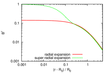
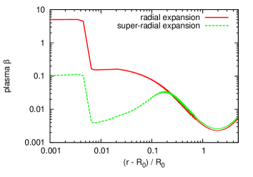
Figure 10.— Snapshots of the profiles of $B^{r}$ and plasma $\beta$ at the initial time. The top panel is $B^{r}$ and the bottom panel is the plasma $\beta$.

In this paper, we adopt super-radially expanding flux tubes, referring to closed loops on the Sun. In the following, we check the effect of this flux tube on the evolution of the magnetosphere plasma. Note that Equation (2) means the funnel structure weakens the magnetic field around $r=R_{1}=2R_{0}$. We adopt a radially expanding flux tube with the same magnetic field strength at the loop top to compare with the case of the super-radially expanding tube we have considered so far: $f(r)=\mathrm{const.},B^{r}\propto 1/r^{2}$. As shown in the top panel of Figure 10, the magnetic field strength of the radially expanding flux tube case near the surface is smaller than that of the super-radial expansion case. This results in larger plasma $\beta$ near the surface.

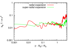
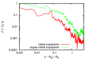
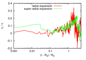
Figure 11.— Top: A snapshot the temperature $k_{B}T/mc^{2}$. Middle: A snapshot of the density $\rho\gamma/\rho_{0}\gamma_{0}$. Bottom: A snapshot of the radial velocity $v_{r}/c$. All snapshots are at $t=10t_{0}$ and we used $r_{g}/R_{0}=0.3$ and $\langle\delta v_{\perp}\rangle=0.75c_{s}$.

Each panel of Figure 11 is the snapshots of the temperature, mass density and radial velocity in the case of $r_{g}/R_{0}=0.3$ and $\langle\delta v_{\perp}\rangle=0.75c_{s}$ at $t=10t_{0}$ comparing with the radially expanding flux tube case. We find that the radial expansion case gives smaller mass density. In particular, the radial velocity in the case of radially-expanding flux tube structure is clearly smaller in the region $r<R_{1}$. This is because the magnetic field with the radially-expanding flux tube is weaker in this region and this makes the Alfvén wave pressure smaller, which results in the smaller mass and energy transfer to the outer region. Note that the smaller mass density near the surface is induced by the aforementioned initial stronger pressure gradient force and does not relate to the Alfvén waves.

Note that if we use the same magnetic field value at the central star surface, the super-radial expansion results in the weaker magnetic field in the outer region and this induces smaller Alfvén wave pressure and mass and energy transfer.

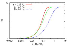
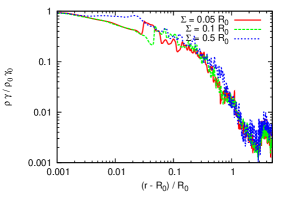
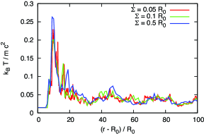
Figure 12.— Left: The configuration of the flux tube with different value of $\Sigma$. Middle: Snapshots of the density profile at $t=10R_{0}/c$. Right: The temporal evolution of temperature at the loop top.

Finally, we discuss the dependence on the parameter $\Sigma$. Equation (1), has three parameters: $R_{1},\Sigma,f_{\mathrm{Max}}$. $R_{1}$ controls the coordinate where the super-radial flux tube expands drastically. This should be determined by the pressure balance, so that we use the same coordinate as the edge of the atmosphere. $f_{\mathrm{Max}}$ determines the strength of the magnetic field in the magnetosphere, and we set this value through the numerical limitation of low-$\beta$ calculations. Concerning $\Sigma$, this parameter determines the characteristic scale of the expansion of the tube as can be seen in the left panel of Figure 12 that is the configuration of flux tubes with different $\Sigma$ values. The middle and right panels of Figure 12 are a snapshot of the density profile at $t=10R_{0}$ and the temporal evolution of temperature at the loop top using different values of $\Sigma$. Within the probable parameter region $\Sigma<R_{1}$, we cannot find any drastic differences in those results.

References

- Amano & Kirk (2013) Amano, T., & Kirk, J. G. 2013, ApJ, 770, 18
- Beckwith & Stone (2011) Beckwith, K., & Stone, J. M. 2011, ApJS, 193, 6
- Beloborodov (2009) Beloborodov, A. M. 2009, ApJ, 703, 1044
- Beloborodov (2013) —. 2013, ApJ, 762, 13
- Beloborodov & Thompson (2007) Beloborodov, A. M., & Thompson, C. 2007, Ap&SS, 308, 631
- Blaes et al. (1989) Blaes, O., Blandford, R., Goldreich, P., & Madau, P. 1989, ApJ, 343, 839
- Duncan (2004) Duncan, R. C. 2004, in Cosmic explosions in three dimensions, ed. P. Höflich, P. Kumar, & J. C. Wheeler, 285
- Duncan & Thompson (1992) Duncan, R. C., & Thompson, C. 1992, ApJ, 392, L9
- Esposito et al. (2007) Esposito, P., et al. 2007, A&A, 476, 321
- Feroci et al. (2004) Feroci, M., Caliandro, G. A., Massaro, E., Mereghetti, S., & Woods, P. M. 2004, ApJ, 612, 408
- Fox et al. (2005) Fox, D. B., et al. 2005, Nature, 437, 845
- Gabler et al. (2012) Gabler, M., Cerdá-Durán, P., Stergioulas, N., Font, J. A., & Müller, E. 2012, MNRAS, 421, 2054
- Gill & Heyl (2010) Gill, R., & Heyl, J. S. 2010, MNRAS, 407, 1926
- Goldstein (1978) Goldstein, M. L. 1978, ApJ, 219, 700
- Harding & Lai (2006) Harding, A. K., & Lai, D. 2006, Reports on Progress in Physics, 69, 2631
- Hurley et al. (2005) Hurley, K., et al. 2005, Nature, 434, 1098
- Ito et al. (2010) Ito, H., Tsuneta, S., Shiota, D., Tokumaru, M., & Fujiki, K. 2010, ApJ, 719, 131
- Kliem & Török (2006) Kliem, B., & Török, T. 2006, Physical Review Letters, 96, 255002
- Kojima & Okita (2004) Kojima, Y., & Okita, T. 2004, ApJ, 614, 922
- Kopp & Holzer (1976) Kopp, R. A., & Holzer, T. E. 1976, Sol. Phys., 49, 43
- Kudoh & Shibata (1999) Kudoh, T., & Shibata, K. 1999, ApJ, 514, 493
- Lamers & Cassinelli (1999) Lamers, H. J. G. L. M., & Cassinelli, J. P. 1999, Introduction to Stellar Winds
- Lyubarsky (2005) Lyubarsky, Y. E. 2005, MNRAS, 358, 113
- Lyutikov (2003) Lyutikov, M. 2003, MNRAS, 346, 540
- Lyutikov (2006) —. 2006, MNRAS, 367, 1594
- Lyutikov & Uzdensky (2003) Lyutikov, M., & Uzdensky, D. 2003, ApJ, 589, 893
- Marti & Muller (1994) Marti, J. M., & Muller, E. 1994, Journal of Fluid Mechanics, 258, 317
- Masada et al. (2010) Masada, Y., Nagataki, S., Shibata, K., & Terasawa, T. 2010, PASJ, 62, 1093
- Matsumoto & Kitai (2010) Matsumoto, T., & Kitai, R. 2010, ApJ, 716, L19
- Mazur & Heyl (2011) Mazur, D., & Heyl, J. S. 2011, MNRAS, 412, 1381
- Mereghetti (2008) Mereghetti, S. 2008, A&A Rev., 15, 225
- Mereghetti et al. (2002) Mereghetti, S., De Luca, A., Caraveo, P. A., Becker, W., Mignani, R., & Bignami, G. F. 2002, ApJ, 581, 1280
- Mereghetti et al. (2005) Mereghetti, S., et al. 2005, ApJ, 628, 938
- Mereghetti et al. (2006) —. 2006, ApJ, 653, 1423
- Mignone & McKinney (2007) Mignone, A., & McKinney, J. C. 2007, MNRAS, 378, 1118
- Mignone et al. (2005) Mignone, A., Plewa, T., & Bodo, G. 2005, ApJS, 160, 199
- Mignone et al. (2009) Mignone, A., Ugliano, M., & Bodo, G. 2009, MNRAS, 393, 1141
- Mochol & Kirk (2013a) Mochol, I., & Kirk, J. G. 2013a, ApJ, 771, 53
- Mochol & Kirk (2013b) —. 2013b, ArXiv e-prints
- Moriyasu et al. (2004) Moriyasu, S., Kudoh, T., Yokoyama, T., & Shibata, K. 2004, ApJ, 601, L107
- Nakagawa et al. (2007) Nakagawa, Y. E., et al. 2007, PASJ, 59, 653
- Okita et al. (2008) Okita, T., Nagataki, S., & Kojima, Y. 2008, Progress of Theoretical Physics, 119, 39
- Olive et al. (2004) Olive, J.-F., et al. 2004, ApJ, 616, 1148
- Pacini (1974) Pacini, F. 1974, Nature, 251, 399
- Parfrey et al. (2013) Parfrey, K., Beloborodov, A. M., & Hui, L. 2013, ApJ, 774, 92
- Piro (2005) Piro, A. L. 2005, ApJ, 634, L153
- Sagdeev & Galeev (1969) Sagdeev, R. Z., & Galeev, A. A. 1969, Nonlinear Plasma Theory
- Shibata & Uchida (1986) Shibata, K., & Uchida, Y. 1986, Sol. Phys., 103, 299
- Suzuki & Inutsuka (2005) Suzuki, T. K., & Inutsuka, S.-i. 2005, ApJ, 632, L49
- Suzuki & Inutsuka (2006) Suzuki, T. K., & Inutsuka, S.-I. 2006, Journal of Geophysical Research (Space Physics), 111, 6101
- Suzuki et al. (2008) Suzuki, T. K., Sumiyoshi, K., & Yamada, S. 2008, ApJ, 678, 1200
- Takamori et al. (2012) Takamori, Y., Okawa, H., Takamoto, M., & Suwa, Y. 2012, ArXiv e-prints
- Takamoto (2013) Takamoto, M. 2013, ApJ, 775, 50
- Tanaka et al. (2007) Tanaka, Y. T., Terasawa, T., Kawai, N., Yoshida, A., Yoshikawa, I., Saito, Y., Takashima, T., & Mukai, T. 2007, ApJ, 665, L55
- Terasawa et al. (1986) Terasawa, T., Hoshino, M., Sakai, J.-I., & Hada, T. 1986, J. Geophys. Res., 91, 4171
- Terasawa et al. (2005) Terasawa, T., et al. 2005, Nature, 434, 1110
- Thompson & Duncan (1995) Thompson, C., & Duncan, R. C. 1995, MNRAS, 275, 255
- Thompson & Duncan (1996) —. 1996, ApJ, 473, 322
- Thompson et al. (2002) Thompson, C., Lyutikov, M., & Kulkarni, S. R. 2002, ApJ, 574, 332
- Tian et al. (2010) Tian, H., Marsch, E., Tu, C., Curdt, W., & He, J. 2010, New A Rev., 54, 13
- Török et al. (2004) Török, T., Kliem, B., & Titov, V. S. 2004, A&A, 413, L27
- Tsuneta et al. (2008) Tsuneta, S., et al. 2008, ApJ, 688, 1374
- Woods et al. (2001) Woods, P. M., Kouveliotou, C., Göǧüş, E., Finger, M. H., Swank, J., Smith, D. A., Hurley, K., & Thompson, C. 2001, ApJ, 552, 748
- Woods & Thompson (2006) Woods, P. M., & Thompson, C. 2006, Soft gamma repeaters and anomalous X-ray pulsars: magnetar candidates, ed. W. H. G. Lewin & M. van der Klis, 547–586
- Yu (2012) Yu, C. 2012, ApJ, 757, 67
- Yu & Huang (2013) Yu, C., & Huang, L. 2013, ApJ, 771, L46
- Zenitani et al. (2010) Zenitani, S., Hesse, M., & Klimas, A. 2010, ApJ, 716, L214