Hydration shell effects in the relaxation dynamics of photoexcited Fe-II complexes in water

Abstract

We study the relaxation dynamics of photoexcited Fe-II complexes dissolved in water and identify the relaxation pathway which the molecular complex follows in presence of a hydration shell of bound water at the interface between the complex and the solvent. Starting from a low-spin state, the photoexcited complex can reach the high-spin state via a cascade of different possible transitions involving electronic as well as vibrational relaxation processes. By numerically exact path integral calculations for the relaxational dynamics of a continuous solvent model, we find that the vibrational life times of the intermittent states are of the order of a few ps. Since the electronic rearrangement in the complex occurs on the time scale of about 100 fs, we find that the complex first rearranges itself in a high-spin and highly excited vibrational state, before it relaxes its energy to the solvent via vibrational relaxation transitions. By this, the relaxation pathway can be clearly identified. We find that the life time of the vibrational states increases with the size of the complex (within a spherical model), but decreases with the thickness of the hydration shell, indicating that the hydration shell acts as an additional source of fluctuations.

I Introduction

When a photoexcited molecule is placed in a polarizable solvent, it will relax its energy in presence of potentially strong interactions with its bath, i.e., its nearest neighbor solvent molecules. This interplay manifests itself already in the properties of the steady state by the observed Stokes shift between the absorption and emission energies of the solute, which typically reflect the rearrangement of the caging solvent around the excited solute Fleming96 ; Ball08 ; Cramer99 . A pioneering femtosecond transient absorption laser study of photoexcited NO in solid Ne and Ar rare gas matrices was capable of extracting mechanistic movements of the caging rare gas atoms in combination with model calculations Jeannin00 ; Vigliotti02 , but in liquid media this connection to the actual solvent movements in response to the creation of an excited state dipole moment is inherently difficult to observe experimentally. Quantum chemical calculations have meanwhile advanced and now permit simulating the dynamic response inside a box containing the excited molecule itself and a certain number of moving solvent molecules. In this way, simple ions Pham11 , but also more complex molecules, such as aqueous [Fe(bpy)₃]²⁺ could be treatedDaku10 . In a recent experiment, Haldrup et al. have attempted to tackle this phenomenon exploiting combined x-ray spectroscopies and scattering tools Haldrup12 . This picosecond time-resolved experiment used x-ray absorption spectroscopy to unravel the electronic changes visible around the Fe $K$ absorption edge. They occur concomitant to the geometric structural changes already extracted from the extended x-ray absorption fine structure (EXAFS) region Gawelda09 . The latter monitors the molecular changes around the central Fe atom. While these studies only shed light on the excited molecular dynamics within itself, the recent study combined x-ray emission spectroscopy (XES) with x-ray diffuse scattering (XDS) to obtain a picture of the internal electronic and structural dynamics (via XES) simultaneously with the geometric structural changes in the caging solvent shell. One surprising result from this experimental campaign has yielded information about a density increase right after photoexcitation (i.e., within the 100 ps time resolution of that study), which was fully in line with the MD simulations of Ref. Daku10, . They calculated a change in the solvation shell between the low spin (LS) ground and high spin (HS) excited state, which resulted in the expulsion of – on average – two water molecules from the solvation shell into the bulk solvent. This showed up in the XDS data as a density increase in the transient XDS pattern, and even the quantitative analysis extracted an average density increase due to about two water molecules expelled into the bulk solvent per photoexcited [Fe(bpy)₃]²⁺.

This success has triggered the current theoretical study: If it is becoming possible to experimentally gain new insight into guest-host interactions in disordered systems like aqueous solutions, would it be possible to eventually understand the influence of guest-host interactions on the dynamic processes occurring within the solute? Indeed, aqueous [Fe(bpy)₃]²⁺ is an ideal model system for several reasons. Internally, it undergoes several ultrafast transition processes involving correlations within the $3d$ orbitals: after photoexcitation from the ¹A₁ ground state into its singlet excited metal-to-ligand charge transfer state (¹MLCT), it rapidly undergoes an intersystem crossing into the triplet manifold (³MLCT) within about 30 fs Cannizzo06 , and leaves the MLCT manifold in 120 fs Gawelda07 . Femtosecond XAS studies observed the appearance of the finally accessed HS ⁵T₂ state in less than 250 fs Bressler09 ; Lemke13 , which was also confirmed by an ultrafast optical-UV transient absorption study Consani09 . A very recent femtosecond XES study revealed the existence of a metal-centered intermediate electronic state on the fly before the system settles into the HS state Zhang14 . This electronic and spin-switching process sequence starts from the LS ground state which is formed by six paired electrons in the lower t_2g level. Then, the cascade proceeds to the HS excited state. There, the six electrons are distributed via t${}_{2g}^{4}$e${}_{g}^{2}$ and both e${}_{g}^{2}$ electrons with parallel spins to two of the four t${}_{2g}^{4}$ electrons. Overall, $S=2$ in the HS state (against $S=0$ in the ground state) results. Such a transition is very common in Fe-II based spin crossover (SCO) compounds, but little is understood about both the internal dynamic processes involved as well as about the possible influence of the solvent on this rapid spin-switching scheme. Indeed, the initially excited MLCT manifold should interact with the caging solvent molecules, but currently little is known about the actual dynamic processes. This mystery motivates the calculations performed in this work.

Here we investigate the energy relaxation dynamics in photoexcited aqueous [Fe(bpy)₃]²⁺ theoretically in order to provide a new view of the short-time guest-host interactions in this complex sequence of relaxation. The water molecules close to the compound are polarized and a hydration shell of bound water is formed. On the one hand, this hydration shell may shield the complex from polarization fluctuations provided by the bulk water. On the other hand, it may also act as an additional source of polarization fluctuations and thus enhance the relaxation process. To be specific here, we consider the case of [Fe(bpy)₃]²⁺ in water Bressler09 ; Haldrup12 ; Daku10 . The set of states which are involved in the cascade of transitions from the LS to the HS state is schematically shown in Fig. 1. Also, several intermediate vibronic states of the complex are relevant Tuchagues04 . An initial photoexcitation (green solid arrow) brings the Fe-II complex from the ground state of the LS configuration into an excited vibronic state of a configuration of the metal-to-ligand-charge-transfer (MLCT) state. The photoexcitation at $400$ nm provides an energy of about $3.1$ eV or $\sim 25000$ cm^-1. More precisely, a state on the ¹MLCT manifold is initially excited, but rapidly undergoes an intersystem crossing into the triplet manifold (³MLCT) within about 30 fs Gawelda07 . The two manifolds are similar in their vibrational frequencies and correspond to the skeleton mode of bpy in the MLCT configuration. This mode has a rather high vibrational frequency of $\Omega_{\rm MLCT}=1607$ cm^-1and its vibrational ground state has an energy of about $18000$ cm^-1. Hence, the photoexcitation populates mostly the vibrational state $|4\rangle_{\rm MLCT}$ with a quantum number $\nu_{MLCT}=4$.

The relaxation out of this state can now occur via two alternative relaxation pathways. Elements of these pathways are known, but the path which is eventually chosen by the system is not fully understood in detail up to present. On the one hand, the relaxation can proceed via energetically lower-lying vibrational states on the MLCT manifold, i.e., following $|4\rangle_{\rm MLCT}\to|3\rangle_{\rm MLCT}\to\dots$ (the blue path, see the sequence of blue arrows in Fig. 1). In fact, the available MLCT states form a broad manifold of metal-centered states Bressler09 . From the MLCT ground state, the energy could be transferred to a vibrationally excited state of one of the metal-centered triplet states (^1/3T). In the T state, the Fe-N bond length increases, such that the Fe-II complex expands by about $0.1$ Å. This molecular configuration has a vibrational energy gap Tuchagues04 of $\Omega_{\rm T}\sim 250$ cm^-1which corresponds to a vibrational mode of the Fe-N bond. It is experimentally well-established that the transfer from the MLCT manifold to the intermediate T states occurs in about $120$ fs. The system would reach the vibrational ground state of the T configuration via a sequence of vibrational relaxation steps. From the T-vibrational ground state, the energy would be transferred to a vibrational excited state of the HS configuration. Its HS vibrational ground state has an energy of $\sim 4000$ cm^-1. The vibrational energy gap is again determined by a vibrational mode of the Fe-N bond and is estimated Tuchagues04 as $\Omega_{\rm HS}\sim 150$ cm^-1. It is established that the transfer from the T to the HS state occurs within $70$ fs Bressler09 ; Zhang14 . Along with this occurs another rearrangement of the compound which results in an effective growth of the molecule (and thus somewhat the caging cluster) of $0.2$ Å. After vibrational relaxation in the HS state, the system would reach its HS ground state configuration within $960$ fs Gawelda07 .

The second possible pathway (the red path, see the sequence of red arrows in Fig. 1) would start in a highly excited vibrational state on the MLCT manifold as before. Without performing a vibrational relaxation transition within the MLCT manifold, it directly yields to a highly excited vibrational state on the T manifold within $120$ fs and continues again without a vibrational relaxation transition to another highly excited vibrational state of the HS configuration within $70$ fs. From there, the complex relaxes into the HS ground state via vibrational transitions and removal of the corresponding energy into the hydration shell and bulk water within $960$ fs Gawelda07 .

The final HS to LS relaxation occurs in $665$ ps Gawelda07 .

Both scenarios would allow the system to reach the HS electronic manifold within roughly $200$ fs via several intermediate states. The initial energy is intermittently stored within molecular vibrations but finally transferred out of the complex into the solvent environment. The Fe-II complex expands, since the Fe-N bond lengths increase, when the compound is excited from the LS to HS state. Here, we assume that Fe-N stretching and bending modes are dominant.

What is unknown from the experimental perspective, is the vibrational life times of the intermediate vibrational electronic states (blue and red question marks in Fig. 1). For instance, if the highly excited vibrational states on the MLCT manifold live long enough such that the transfer to the T-manifold can occur within $120$ fs, the system would most likely choose the red pathway. On the other hand, if the highly excited vibrational states on the MLCT manifold rapidly relax within $120$ fs to the MLCT ground state, the system would prefer to follow the blue relaxation pathway.

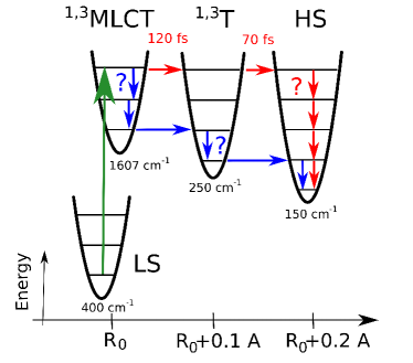
Figure 1: Sketch of the energies of the LS, MLCT, T and the HS state (not to scale). The details are given in the text. The two possible relaxation pathways are indicated by the sequences of the red and blue arrows. The unknown life time of the vibrational states is indicated by the blue question mark and is determined in this work.

To decide this question from a theoretical point of view, we follow a simplified model description which is accurate enough such that a clear qualitative answer follows. For this, we establish a model of a quantum mechanical two-state system which describes a bath-induced vibrational relaxation from an excited vibrational state to the ground state on a generic manifold. We thereby model the environmental polarization fluctuations including the effects of a hydration shell in terms of a refined Onsager model combined with a Debye relaxation picture Abe . A crucial aspect here is that we include the bulk solvent and the hydration shell on the same footing in terms of a continuum description of environmental Gaussian modes. This model allows us easily to modify the radius of the solvated complex (taken as a sphere in this work) and the thickness of the surrounding hydration shell. Within this simplified model, we determine the energy relaxation rate for several representative vibrational modes including the Fe-N stretching and bending modes in dependence of the Fe-N bond length and the hydration shell thickness. Technically, we use numerically exact real-time path integral simulations on the basis of a fluctuational spectrum which is highly structured and far from being Ohmic. Such a “slow” bath reflects the similar physical time scales on which the vibrational relaxation transitions within a vibrational manifold and the polarization fluctuations of the surrounding water occur. The highly non-Ohmic form (see below) of the bath spectral densities a priori calls for the use of an advanced theoretical method beyond the standard Markov-approximated dynamical Redfield equations.

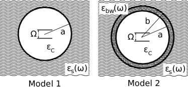
Figure 2: Sketch of continuum dielectric models for the complex-bound-water-solvent system, see text for details. $a$ denotes the radius of the inner sphere, while $b$ refers to the radius of the outer sphere. $\varepsilon_{\rm s}(\omega)$ is the frequency-dependent complex dielectric function of the continuum bulk water modes. $\varepsilon_{\rm bw}(\omega)$ is the frequency-dependent complex dielectric function associated with the bound water shell. $\varepsilon_{c}=1$ is the dielectric constant of the vacuum inside the cavity.

We find vibrational energy relaxation times on generic manifolds in the range of $2-8$ ps depending on the Fe-N bond lengths and the hydration shell thickness. For this, we tune the vibrational frequencies which are determined by the curvature of the manifolds over a relevant parameter range. We can determine the modes with fastest energy relaxation which dominates the energy relaxation dynamics of the Fe-II complex since internal energy redistribution is likely much faster. Most importantly, we observe that the vibrational relaxation times within a manifold are much longer than the typical time scales of a few hundred fs during which the HS state is formed. Two effects are competing here. A complex with a smaller radius of the solvation sphere brings the environmental fluctuations spatially closer to the complex and thus results in a faster decay. However, in turn, the stronger Fe-N bond results in larger mode frequencies. Overall, the calculated life times of the vibrationally excited states in the ps regime clearly show that the vibrational life times are much longer than the complex overall needs to reach the HS state, which are less than $200$ fs. Thus, we can conclude that the energy relaxation basically occurs via the “red pathway” after the complex has reached the HS state and vibrationally relaxes into the ground state.

II Model

To determine the life time of the excited vibrational states, we formulate a minimal model in form of a quantum two-level system which is immersed in its solvent environment (model 1) and is, in addition, surrounded by a hydration shell (model 2). After expansion of the Fe-II complex, the stretching and bending modes Sousa2013 involving the Fe-N bond change their respective vibrational frequency. We investigate their relaxation dynamics independently and use the spin-boson Hamiltonian Weiss as a minimal model, i.e.,

$$H=\frac{\hbar\Omega}{2}\sigma_{z}+\hbar\sigma_{x}\sum_{j}c_{j}(b_{j}+b_{j}^{\dagger})+\sum_{j}\hbar\omega_{j}b_{j}^{\dagger}b_{j}\,.$$ (1)

Here, the Pauli matrix $\sigma_{z}$ contains the ground state $|g\rangle$ and the excited state $|e\rangle$ between which we investigate the relaxation transitions. The two states are separated in energy by the vibrational frequency $\Omega$. The bath modes produce Gaussian fluctuations stemming from harmonic oscillators with frequencies $\omega_{j}$, the corresponding creation and destruction operators of the bath modes are denoted as $b_{j}^{\dagger}$ and $b_{j}$. The fluctuations induce transitions in the system via the Pauli matrix $\sigma_{x}$. They can be characterized by a single function Weiss , the spectral density

$$J(\omega)=2\pi\sum_{j}c_{j}^{2}\delta(\omega-\omega_{j})\,.$$ (2)

It provides the spectral weight contained in the fluctuations at frequency $\omega$ which are provided by a Gaussian bath at thermal equilibrium at a given fixed temperature $T=1/(k_{B}\beta)$. The correlation function of the quantum bath fluctuations $\xi(t)$ is given by ($t>0$)

$$\langle\xi(t)\xi(0)\rangle=\frac{1}{\pi}\int_{0}^{\infty}d\omega J(\omega)\left[\coth\frac{\hbar\omega\beta}{2}\cos\omega t-i\sin\omega t\right]\,.$$ (3)

This quantity determines the relaxation and dephasing rates Weiss . In this work, we consider several representative Fe-N stretching and bending modes with the frequencies $\Omega=$ 60, 120, 150, and 250 cm^-1. Moreover, we use a continuum description of the solvent (bulk) water and the hydration shell following Gilmore and McKenzie Gilmore08 . The key quantity to characterize the environment, i.e., the spectral distribution $J(\omega)$ of the fluctuations, is determined in terms of the standard Onsager model of polarization fluctuations of the solvent water molecules. Their relaxation properties are described within a Debye relaxation picture Abe . In this approach, the spectral density is related to the continuum dielectric function $\varepsilon(\omega)$ of the host material.

To be more specific, we consider two different situations Gilmore08 , see Fig. 2: In model 1, we assume that the complex with its vibrational mode is placed inside a vacuum spherical cavity of radius $r_{a}$ with a dielectric constant $\varepsilon_{c}=1$. This is situated in a continuum of bulk water modes with a frequency-dependent complex dielectric function $\varepsilon_{\rm s}(\omega)$. In model 2, we add to model 1 an outer sphere with radius $r_{b}>r_{a}$. The shell formed by the two spheres describes the bound water or hydration shell in terms of a second frequency-dependent complex dielectric function $\varepsilon_{\rm bw}(\omega)$. This model allows us to determine the relaxation rates also for varying the radii $r_{a}$ and $r_{b}$ independently. Throughout this work, we set $T=300$ K.

II.1 Model 1: Bulk water

Following Gilmore and McKenzie Gilmore08 ; Gilmore05 , one can calculate the reaction field by solving Maxwell’s equation for the particular geometry shown in Fig. 2. This yields the spectral density

$$J_{1}(\omega) = \frac{(\Delta\mu)^{2}}{2\pi\varepsilon_{0}r_{a}^{3}}{\rm Im}\frac{\varepsilon_{\rm s}(\omega)-1}{2\varepsilon_{\rm s}(\omega)+1}$$ (4)

$$= \frac{(\Delta\mu)^{2}}{2\pi\varepsilon_{0}r_{a}^{3}}\frac{6(\varepsilon_{{\rm s},0}-\varepsilon_{{\rm s},\infty})}{(2\varepsilon_{{\rm s},0}+1)(2\varepsilon_{{\rm s},\infty}+1)}\frac{\omega\tau_{\rm s}}{\omega^{2}\tau_{\rm s}^{2}+1}\,,$$

with the respective transition dipole moment $\Delta\mu$ of the vibration, $\varepsilon_{{\rm s},0}$ being the static dielectric constant of the bulk solvent, $\varepsilon_{{\rm s},\infty}$ being the high-frequency dielectric constant of the bulk solvent, and

$$\tau_{\rm s}=\frac{2\varepsilon_{{\rm s},\infty}+1}{2\varepsilon_{{\rm s},0}+1}\tau_{\rm D,s}$$ (5)

and $\tau_{\rm D,s}$ is the Debye relaxation time of the solvent. For water, we have $\varepsilon_{{\rm s},0}=78.3,\varepsilon_{{\rm s},\infty}=4.2$ and $\tau_{\rm D,s}=8.2$ ps.

Here, we are interested in the dependence of the spectral density on the cavity volume determined by its radius $a$ and we thus collect all constants in a prefactor. We arrive at

$$J_{1}(\omega)=\frac{\alpha_{1}}{a^{3}}\frac{\omega}{\omega^{2}\tau_{\rm s}^{2}+1}\,,$$ (6)

with

$$\alpha_{1}=\frac{1}{2\pi\hbar}\frac{(\Delta\mu)^{2}}{2\pi\varepsilon_{0}a_{0}^{3}}\frac{6(\varepsilon_{{\rm s},0}-\varepsilon_{{\rm s},\infty})}{(2\varepsilon_{{\rm s},0}+1)(2\varepsilon_{{\rm s},\infty}+1)}\tau_{\rm s}\,,$$ (7)

where $a_{0}$ is the typical length scale of the problem and where the now dimensionless radius $a=r_{a}/a_{0}$ is measured in units of $a_{0}$. We fix this to $a_{0}=1$ Å throughout this work. The spectrum is purely Ohmic Weiss with a cut-off frequency given by $\omega_{\rm c,s}=1/\tau_{\rm s}$. For our considerations, we fix the dipole moment to a typical value of $\Delta\mu=1$ D $=3\times 10^{-30}$ Cm. Collecting all parameters yields $\alpha_{1}\approx 5$ for bulk water.

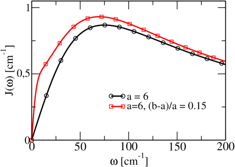
Figure 3: Spectral densities for model 1 (black line, circles) and model 2 (red line, squares) for water and for a cavity radius of $r_{a}=6$ Å and a relative shell thickness of $(b-a)/a=0.15$.

Fig. 3 shows $J_{1}(\omega)$ of model 1 for the case $a=6$ (corresponding to $r_{a}=6$ Å). Maximal spectral weight is observed at roughly 70 cm^-1. Hence, it is clear that the resulting bath correlation times are comparable to or exceed internal system periods. This also prevents us from using a standard Markov approximation a priori, since a correlated and non-Markovian dynamics can in principle be expected Nalbach-JCP-2010 (see below).

II.2 Model 2: Bulk water plus hydration shell

We also include the hydration shell of bound water and do this by a second sphere with outer radius $r_{b}=ba_{0}$ with $b$ being the corresponding dimensionless number. We assume that the hydration shell is thin relative to the radius of the inner sphere and may then perform a Taylor expansion in the relative shell thickness $(b-a)/a$. The resulting spectral density Gilmore08 is

$$J_{2}(\omega)=J_{1}(\omega)+J_{\rm bw}(\omega)\,,$$ (8)

with

$$J_{\rm bw}(\omega) = \frac{(\Delta\mu)^{2}}{2\pi\varepsilon_{0}r_{a}^{3}}\frac{1}{(2\varepsilon_{\rm s}(\omega)+1)^{2}}\left(1+\frac{2\varepsilon_{{\rm s},0}}{|\varepsilon_{\rm bw}(\omega)|^{2}}\right){\rm Im}\varepsilon_{\rm bw}(\omega)\,,$$

where $\varepsilon_{\rm bw}(\omega)$ is the complex dielectric function of the bound water layer. Within the Debye relaxation model, we find

$$J_{\rm bw}(\omega)=\frac{\alpha_{\rm bw}}{a^{3}}\frac{b-a}{a}\frac{\omega}{{\omega}^{2}\tau_{\rm bw}^{2}+1}$$ (10)

with

$$\alpha_{\rm bw}=\frac{1}{2\pi\hbar}\frac{3(\Delta\mu)^{2}}{2\pi\varepsilon_{0}a_{0}^{3}}\frac{(\varepsilon_{{\rm bw},0}^{2}+\varepsilon_{{\rm s},0}^{2})(\varepsilon_{{\rm bw},0}-\varepsilon_{{\rm bw},\infty})}{\varepsilon_{{\rm bw},0}^{2}(2\varepsilon_{{\rm s},0}+1)^{2}}\tau_{\rm bw}\,.$$ (11)

Here, we have the static dielectric constant $\varepsilon_{{\rm bw},0}$ and the high-frequency dielectric constant $\varepsilon_{{\rm bw},\infty}$ of the bound water layer. From generic considerations Gilmore08 , one may infer that the relaxation time of the bound water shell is one order of magnitude large than the solvent relaxation time, i.e., we set $\tau_{\rm bw}=10\tau_{\rm s}$. Likewise, we know Gilmore08 that $\varepsilon_{{\rm s},0}\gg\varepsilon_{{\rm s},\infty}$. Moreover, $\varepsilon_{{\rm bw},0}\gg\varepsilon_{{\rm bw},\infty}$ and $\varepsilon_{{\rm s},0}\gg\varepsilon_{{\rm bw},0}$. Hence, we may use this and set $\varepsilon_{{\rm bw},0}=1$ to obtain

$$\alpha_{\rm bw}=\frac{1}{2\pi\hbar}\frac{3(\Delta\mu)^{2}}{2\pi\varepsilon_{0}a_{0}^{3}}\frac{1}{4}\tau_{\rm bw}\,.$$ (12)

For the parameters mentioned, we find $\alpha_{\rm bw}\approx 118$.

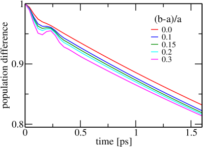
Figure 4: Time evolution of the population difference $P(t)$ for $\Omega=150$ cm^-1for $T=300$ K for different values $(b-a)/a$ of the shell thickness.

Fig. 3 shows $J_{2}(\omega)$ for these parameters and for $a=6$ and $(b-a)/a=0.15$. Again, maximal spectral weight is observed at roughly 70 cm^-1. In general, the spectral weight of model 2 is higher than of model 1. This already indicates that within the continuum approach, the bound water shell acts as an additional source of fluctuations and not as a spectral filter for the continuous bulk modes. Hence, the calculated relaxation times for model 2 will be faster than for model 1.

Moreover, it is clear that the vibrational life times on the MLCT manifold are much larger since there the spectral weight of the solvent environmental modes around the frequency of $\Omega_{\rm MLCT}=1607$ cm^-1  is strongly suppressed (in fact, we do not consider the vibrational relaxation around this frequency in this work).

III Real-time dynamics of the relaxation transitions

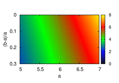
Figure 5: Relaxation time (color scale in ps) of the excited vibrational state for varying radius $r_{a}=aa_{0}$ with $a_{0}=1$ Å    and for varying relative shell thickness $(b-a)/a$ for $\Omega=$150 cm^-1. Model 1 with no hydration shell is contained via the cut along the line $(b-a)/a=0$.

To investigate the quantum relaxation dynamics of the two vibrational states under the influence of environmental fluctuations, we employ the numerically exact quasi-adiabatic propagator path-integral (QUAPI) Makri-JCP-1995 scheme which we have extended to allow treatment of multiple baths Nalbach-NJP-2010 . Specifically, QUAPI is able to treat highly structured and non-Markovian baths efficiently Nalbach-JPB-2012 ; MujicaMoQPRL13 ; MujicaPRE2013 . It determines the time dependent statistical operator $\rho(t)$ which is obtained after the harmonic bath modes have been integrated over. We briefly summarize here the main ideas of this well-established method and refer to the literature for further details. The algorithm is based on a symmetric Trotter splitting of the short-time propagator ${\cal K}(t_{k+1},t_{k})$ for the full Hamiltonian Eq. (1) into a part depending on the system Hamiltonian alone and a part involving the bath and the coupling term. The short-time propagator gives the time evolution over a Trotter time slice $\delta t$. This splitting in discrete time steps is exact in the limit $\delta t\to 0$, i.e., when the discrete time evolution approaches the limit of a continuous evolution. For any finite time slicing, it introduces a finite Trotter error which has to be eliminated by choosing $\delta t$ small enough such that convergence is achieved. On the other side, the environmental degrees of freedom generate correlations being non-local in time. We want to avoid any Markovian approximation at this point and take these correlations into account on an exact footing. We may, however, use the fact that for any finite temperature, these correlations decay exponentially quickly on a time scale denoted as the memory time scale. The QUAPI scheme now defines an object called the reduced density tensor. It corresponds to an extended quantum statistical operator of the system which is nonlocal in time since it lives on this memory time window. By this, one can establish an iteration scheme by disentangling the dynamics in order to extract the time evolution of this object. All correlations are fully included over the finite memory time $\tau_{\rm mem}=K\delta t$, but are neglected for times beyond $\tau_{\rm mem}$. To obtain numerically exact results, we have to increase accordingly the memory parameter $K$ until convergence is found. The two strategies to achieve convergence, i.e., minimize $\delta t$ but maximize $\tau_{\rm mem}=K\delta t$, are naturally counter-current, but nevertheless convergent results can be obtained in a wide range of parameters, including the cases presented in this work.

IV Results

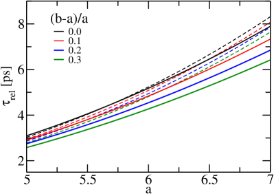
Figure 6: Solid lines: Cut through the 2D plot of Fig. 5 along the lines $(b-a)/a=0,0.1,0.2$ and $0.3$. The dashed lines indicate the results of the vibrational life times calculated within a Born-Markov approximation (see text).

At first, we consider modes with a vibrational frequency of $\Omega=$150 cm^-1. We determine the difference $P(t)=\langle\sigma_{z}\rangle_{t}={\rm tr}[\rho(t)\sigma_{z}]$ of the populations of the ground and the excited states. We start out from the initial preparation of the excited state, i.e., $\rho(0)=|e\rangle\langle e|$. Fig. 4 shows examples of the relaxation dynamics for the environmental models 1 and 2 for different values of the shell thickness $(b-a)/a$. We mainly observe exponential relaxation on a time scale of a few picoseconds. For an increasing shell thickness, a tendency towards a decaying oscillatory dynamics appears. A pronounced oscillation with a period of $\sim 250$ fs develops for the largest thickness considered.

To quantify the decay in terms of life times of the excited state, we extract from the time evolution the corresponding rate by a fit to an exponential. Fig. 5 shows the relaxation time in ps (colour scale) as a function of the radius $a$ of the complex varying it between 5 to 7 Å and the relative shell thickness $(b-a)/a$ varying it between 0 to 30%, which is consistent with the numerical findings of Ref. Daku10, . The plot shows results of both, models 1 and 2 (model 1 corresponds to the line with $(b-a)/a=0$). The data for $(b-a)/a=0,0.1,0.2$ and $0.3$ are shown again in Fig. 6 for better readability. The calculated relaxation times or life times of the excited state vary from $2$ to $8$ ps. For a larger complex radius, the life time increases as expected since the prefactor of the spectral density decreases proportional to $1/r_{a}^{3}$. This reflects the assumption that the effective transition dipole sits in the center of the sphere and an increasing complex pushes the solvent fluctuations further away. This reduces their strength due to the distance dependence of the dipolar coupling. Moreover, the life times decrease with increasing hydration shell thickness. Thus, the hydration shell does not act as a shield from bulk solvent fluctuations but acts as an additional source of fluctuations instead.

Fig. 6 also shows the results of the vibrational life times calculated within a Born-Markov approximation Weiss . The inverse life time or the relaxation rate can be obtained after expanding the transition rates in a master equation approach up to lowest order in the system-bath interaction, together with a Markovian approximation of the bath-induced correlations. This corresponds effectively to only including single-phonon transitions in the bath. The inverse vibrational life time then follows as

$$\tau^{-1}=J(\Omega)\coth\frac{\hbar\Omega\beta}{2}\,.$$ (13)

As is shown by the dashed lines in Fig. 6, significant deviations from the exact life times occur and the approximated life times are overestimated by up to $10\%$.

Next, we show the results for the calculated life times for other vibrational frequencies, i.e., for $\Omega=60,120,150$, and $250$ cm^-1 in Fig. 7.

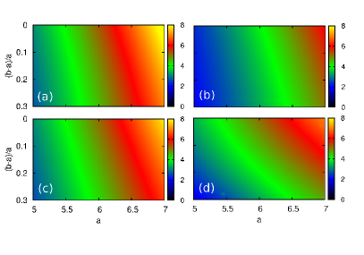
Figure 7: Vibrational life times (color scale in ps) for $\Omega=60$ cm^-1(a), $120$ cm^-1(b), $150$ cm^-1(c) and $250$ cm^-1(d) for models 1 and 2 for $T=300$ K.

These values span the regime of the vibrational frequencies for the Fe-N stretching and bending modes in the LS and HS state Sousa2013 . Note that the frequencies are comparable to or larger than the frequency for which the maximal spectral weight in the environmental fluctuation spectrum occurs. Hence, the energy relaxation dynamics occurs in the regime in which non-Markovian multi-phonon transitions already are noticeable Nalbach-JCP-2010 . We note that for larger values of $\Omega$, no convergent results have been achieved, which is a further strong indication of non-Markovian behavior.

V Conclusions

We observe that under the assumption of equal strengths of the coupling to the environmental fluctuations, all Fe-N stretching and bending modes in the LS and HS state exhibit quite similar vibrational life times on the order of 5 ps. The vibrational energy gap has been modified from $60$ to $250$ cm^-1and all cases show similar results. An increased radius of the complex results in a larger life time since the fluctuating solvent molecules are moved further outside. A finite hydration shell thickness reduces the vibrational life times noticeably.

Our results indicate that all vibrational modes contribute similarly to the energy relaxation after initial photoexcitation. At the same time, all vibrational modes live too long in order to relax the energy already in the MLCT or the T state (assuming here the vibrational modes being identical to the modes in the LS state). Hence, the energy after the photoexcitation is first rapidly transfered from a highly excited vibrational MLCT state to a highly excited vibrational T state and then further to a highly excited vibrational HS state within about less than $200$ fs. Only then, the full excess energy is dissipated while the electronic subsystem is in the HS state. Hence, the system follows the “red relaxation pathway” sketched in Fig. 1.

Energy redistribution within more molecular vibrational states is not included in our simplified model. Assuming the excess energy initially equally distributed among the Fe-N stretching and bending modes Sousa2013 , each mode gets roughly an excitation energy of 440 cm^-1. This implies that roughly two excitations of the mode $\Omega=$ 250 cm^-1 and up to three or four excitations of the mode with $\Omega=$ 120 cm^-1 and $\Omega=$ 150 cm^-1 occur. Thus, the total equilibration time of the complex after photoexcitation roughly follows as three times $5$ ps which yields a value of $15$ ps. These results could be experimentally verified by ultrafast spectroscopy of the intermediate MLCT and T states.

VI Acknowledgments

We acknowledge financial support by the DFG Sonderforschungsbereich 925 “Light-induced dynamics and control of correlated quantum systems” (projects A4 and C8) and by the DFG excellence cluster “The Hamburg Center for Ultrafast Imaging”. CB, AG, WG acknowledge funding by the European XFEL.

References

- (1) G.R. Fleming and M. Cho, Annu. Rev. Phys. Chem. 47, 109 (1996).
- (2) P. Ball, Chem. Rev. 108, 74 (2008).
- (3) C. Cramer and D. Truhlar, Chem. Rev. 99, 2161 (1999).
- (4) C. Jeannin, M.T. Portella-Oberli, S. Jiminez, F. Vigliotti, B. Lang, and M. Chergui, Chem. Phys. Lett. 316, 51 (2000).
- (5) F. Vigliotti, L. Bonacina, M. Chergui, G. Rojas-Lorenzo, and J. Rubayo-Soneira, Chem. Phys. Lett. 362, 31 (2002).
- (6) V.-T. Pham, Thomas J. Penfold, R. M. van der Veen, F. Lima, A. El Nahhas, S. Johnson, R. Abela, C. Bressler, I. Tavernelli, C. J. Milne, and M. Chergui, J. Am. Chem. Soc. 133, 12740 (2011).
- (7) L.M.L. Daku and A. Hauser, J. Phys. Chem. Lett. 1, 1830 (2010).
- (8) K. Haldrup, G. Vankó, W. Gawelda, A. Galler, G. Doumy, A. M. March, E. P. Kanter, A. Bordage, A. Dohn, T. B. van Driel, K. S. Kjaer, H. T. Lemke, S. E. Canton, J. Uhlig, V. Sundström, L. Young, S. Southworth, M. M. Nielsen, and C. Bressler, J. Chem. Phys. A116, 9878 (2012).
- (9) W. Gawelda, V.-T. Pham, R. M. van der Veen, D. Grolimund, R. Abela, M. Chergui, and C. Bressler, J. Chem. Phys. 130, 124520 (2009).
- (10) A. Cannizzo, F. Van Mourik, W. Gawelda, M. Johnson, F. M. F. deGroot, R. Abela, C. Bressler, and M. Chergui, Angew. Chem. Intl. Ed. 45, 3174 (2006).
- (11) W. Gawelda, A. Cannizzo, V.-T. Pham, F. Van Mourik, C. Bressler, and M. Chergui, J. Am. Chem. Soc. 129, 8199 (2007).
- (12) H. T. Lemke, C. Bressler, L.X. Chen, D.M. Fritz, K.J. Gaffney, A. Galler, W. Gawelda, K. Haldrup, R. W. Hartsock, H. Ihee, J. Kim, K. H. Kim, J. H. Lee, M. M. Nielsen, A. B. Stickrath, W. Zhang, D. Zhu, and M. Cammarata, J. Phys. Chem. A117, 735 (2013).
- (13) Ch. Bressler, C. Milne, V.-T. Pham, A. ElNahhas, R.M. van der Veen, W. Gawelda, S. Johnson, P. Beaud, D. Grolimund, M. Kaiser, C.N. Borca, G. Ingold, R. Abela, and M. Chergui, Science 323, 489 (2009).
- (14) C. Consani, M. Prémont-Schwarz, A. El Nahhas, C. Bressler, F. Van Mourik, and M. Chergui, Angew. Chem. Int. Ed. 48, 7184 (2009).
- (15) W Zhang, R. Alonso-Mori, U. Bergmann, C. Bressler, M. Chollet, A. Galler, W. Gawelda, R. G. Hadt, R. W. Hartsock, T. Kroll, K. S. Kjær, K. Kubiček, H. T. Lemke, H. W. Liang, D. A. Meyer, M. M. Nielsen, C. Purser, J. S. Robinson, E. I. Solomon, Z. Sun, D. Sokaras, T. B. van Driel, G. Vankó, T. Weng, D. Zhu, and K. J. Gaffney, Nature (in press 2014).
- (16) J.P. Tuchagues, A. Bousseksou, G. Molnar, J.J. McGarvey, and F. Varret, Top. Curr. Chem. 235, 55 (2004).
- (17) A. Nitzan, Chemical Dynamics in Condensed Phases: Relaxation, Transfer, and Reactions in Condensed Molecular Systems (Oxford University Press, Oxford, 2006).
- (18) C. Sousa, C. de Graaf, A. Rudaskyi, R. Broer, J. Tatchen. M. Etinski, and C. M. Marian, Chem. Eur. J. 19, 17541 (2013).
- (19) U. Weiss, Quantum Dissipative Systems, 4th ed. (World Scientific, Singapore, 2012).
- (20) J. Gilmore and R.H. McKenzie, J. Phys. Chem. A 112, 2162 (2008).
- (21) J. Gilmore and R.H. McKenzie, J. Phys.: Condens. Matter 17, 1735 (2005).
- (22) P. Nalbach and M. Thorwart, J. Chem. Phys. 132, 194111 (2010).
- (23) N. Makri and D. E. Makarov, J. Chem. Phys. 102, 4600 (1995); ibid., 4611 (1995).
- (24) P. Nalbach, J. Eckel, and M. Thorwart, New J. Phys. 12, 065043 (2010).
- (25) C.A. Mujica-Martinez, P. Nalbach, and M. Thorwart, Phys. Rev. Lett. 111, 016802 (2013).
- (26) P. Nalbach and M. Thorwart, J. Phys. B: At. Mol. Opt. Phys, 45, 154009 (2012).
- (27) C. A. Mujica-Martinez, P. Nalbach, and M. Thorwart, Phys. Rev. E 88, 062719 (2013).