Abstract

Signatures of the $SO(5)\times U(1)$ gauge-Higgs unification at LHC and future colliders are explored. The Kaluza-Klein (KK) mass spectra of $\gamma,Z,Z_{R}$ and the Higgs self-couplings obey universality relations with the Aharonov-Bohm phase $\theta_{H}$ in the fifth dimension. The current data at low energies and at LHC indicate $\theta_{H}<0.2$. Couplings of quarks and leptons to KK gauge bosons are determined. Three neutral gauge bosons, the first KK modes $Z_{R}^{(1)}$, $Z^{(1)}$, and $\gamma^{(1)}$, appear as $Z^{\prime}$ bosons in dilepton events at LHC. For $\theta_{H}=0.114$, the mass and decay width of $Z_{R}^{(1)}$, $Z^{(1)}$, and $\gamma^{(1)}$ are (5.73, 482), (6.07, 342), and (6.08 TeV, 886 GeV), respectively. For $\theta_{H}=0.073$ their masses are 8.00 $\sim$ 8.61 TeV. An excess of events in the dilepton invariant mass should be observed in the $Z^{\prime}$ search at the upgraded LHC at 14 TeV.

1 INTRODUCTION

The discovery of the Higgs boson of a mass around 126 GeV[1, 2] supports the scenario of unification of forces and symmetry breaking envisioned in the standard model (SM) of electroweak interactions. Experimental data so far are consistent with what the SM describes, but more data are necessary to pin down whether or not the discovered boson is definitively the Higgs boson in the SM. Other scenarios such as supersymmetric models[3, 4], little Higgs models[5]-[8], composite Higgs models[9]-[16], warped extra-dimension models[17]-[19], and UED models[20]-[26] have been proposed in anticipation of physics beyond the SM. It is urgent to derive and predict new phenomena which can be observed and checked in the experiments at the upgraded 14 TeV LHC.

The gauge-Higgs unification is formulated in higher-dimensional gauge theory [27]-[32]. The four-dimensional Higgs boson appears as a part of the extra-dimensional component of gauge fields, being unified with four-dimensional gauge fields such as $W$, $Z$ and $\gamma$. Dynamics of the Higgs boson are governed by the gauge principle. Most viable is the $SO(5)\times U(1)$ gauge-Higgs unification in the Randall-Sundrum warped space[9],[33]-[37]. At low energies it yields almost the same physics as the SM, being consistent with LHC data and others. Higgs couplings to gauge bosons, quarks and leptons at the tree level are suppressed by a common factor $\cos\theta_{H}$, where $\theta_{H}$ is the Aharonov-Bohm phase in the extra dimension[38]. All of the precision measurements[9, 39], the tree-unitary constraint[40], and the $Z^{\prime}$ search[41]-[43] indicate $\theta_{H}<0.2$. Branching fractions of various decay modes of the Higgs boson remain nearly the same as in the SM, and the signal strengths of the Higgs decay modes relative to the SM are $\sim\cos^{2}\theta_{H}$[37]. We note that though the gauge-Higgs unification model has similarity to the composite Higgs models, it is more restrictive and has more predictive power.

To distinguish the gauge-Higgs unification from the SM we examine the prediction of new particles. It has been pointed out that the first Kaluza-Klein (KK) modes of $Z$ and $\gamma$, denoted as $Z^{(1)}$ and $\gamma^{(1)}$, must appear around 6 TeV for $\theta_{H}\sim 0.1$. In this paper we give detailed analysis of production of $Z_{R}^{(1)}$, $Z^{(1)}$ and $\gamma^{(1)}$ at the upgraded LHC. Here $Z_{R}$ is the gauge boson associated with $SU(2)_{R}$, which does not have a zero mode. It will be shown that $Z_{R}^{(1)}$, $Z^{(1)}$ and $\gamma^{(1)}$ have large widths and can be seen as $e^{+}e^{-}$ or $\mu^{+}\mu^{-}$ signals. Once their masses are determined, the value of $\theta_{H}$ is fixed from the universality relations, which leads to further prediction of the Higgs self-couplings, etc.. Many other signals of gauge-Higgs unification have been discussed in the literature[44]-[67].

In Sec.2 the action of the model is given. In addition to quark-lepton multiplets in the vector representation of $SO(5)$, fermion multiplets in the spinor representation of $SO(5)$ are introduced to realize the observed unstable Higgs boson. In Sec.3 the effective potential $V_{\rm eff}(\theta_{H})$ is evaluated and relevant parameters of the model are determined. It is shown that there appear universality relations among $\theta_{H}$, the KK mass scale $m_{\rm KK}$, $m_{Z_{R}^{(1)}}$, $m_{Z^{(1)}},m_{\gamma^{(1)}}$, and Higgs cubic and quartic couplings. In Sec.4 dilepton ($e^{+}e^{-},\mu^{+}\mu^{-}$) signals at LHC in the so-called $Z^{\prime}$ search are examined. In the $SO(5)\times U(1)$ gauge-Higgs unification $Z_{R}^{(1)}$, $Z^{(1)}$ and $\gamma^{(1)}$ appear as $Z^{\prime}$ bosons. Their masses are around 6 TeV (8 TeV) for $\theta_{H}=0.114$ (0.073), and they have large decay widths. We show that they must be found in the upgraded LHC at 14 TeV. Sec.5 is devoted to conclusions. In the Appendixes we summarize KK mass spectra, wave functions and gauge couplings of gauge fields, quark-leptons, and $SO(5)$-spinor fermions.

2 MODEL

The model is defined in the Randall-Sundrum warped spacetime [17] with the metric

$$ds^{2}=G_{MN}dx^{M}dx^{N}=e^{-2\sigma(y)}\eta_{\mu\nu}dx^{\mu}dx^{\nu}+dy^{2}~{},$$ (2.1)

where $\eta_{\mu\nu}=\text{diag}(-1,1,1,1)$, $\sigma(-y)=\sigma(y)$, $\sigma(y+2L)=\sigma(y)$ and $\sigma(y)=k|y|$ for $|y|\leq L$. The Planck brane and TeV brane are located at $y=0$ and $y=L$, respectively. In the bulk region, $0<y<L$, the cosmological constant is given by $\Lambda=-6k^{2}$. The warp factor $z_{L}=e^{kL}$ is large; $z_{L}\gg 1$. The KK mass scale is given by $m_{{\rm KK}}=\pi k/(z_{L}-1)\sim\pi kz_{L}^{-1}$. In the fundamental region $0\leq y\leq L$ the metric can be written, in terms of the conformal coordinate $z=e^{ky}$, as

$$ds^{2}=\frac{1}{z^{2}}\Big{(}\eta_{\mu\nu}dx^{\mu}dx^{\nu}+\frac{dz^{2}}{k^{2}}\Big{)}~{}.$$ (2.2)

The gauge symmetry in the bulk region is given by $SO(5)\times U(1)_{X}\times SU(3)_{C}$ with the corresponding gauge fields $A_{M}$, $B_{M}$ and $G_{M}$ and gauge couplings $g_{A},g_{B}$ and $g_{C}$. Quark-lepton multiplets $\Psi_{a}$ are introduced in the vector representation 5 of $SO(5)$, whereas additional fermions $\Psi_{F_{i}}$ are introduced in the spinor representation 4 of $SO(5)$[34, 36, 37]. The $SO(5)$ gauge symmetry is partially broken to $SO(4)\simeq SU(2)_{L}\times SU(2)_{R}$ by orbifold boundary conditions. On the Planck brane at $y=0$ ($z=1$) there live right-handed brane fermions $\hat{\chi}_{\alpha R}$ and brane scalar $\hat{\Phi}$, which are (2,1) and (1,2) representation of $SU(2)_{L}\times SU(2)_{R}$, respectively. The brane interactions are manifestly gauge-invariant under $SO(4)\times U(1)_{X}\times SU(3)_{C}$. The brane scalar $\hat{\Phi}$ spontaneously breaks $SU(2)_{R}\times U(1)_{X}$ to $U(1)_{Y}$ by $\raise 0.68889pt\hbox{$\langle$}\lower 0.68889pt\hbox{}\hat{\Phi}\raise 0.68889pt\hbox{$\rangle$}\lower 0.68889pt\hbox{}\gg m_{\rm KK}$, which, in turn, induces mixing among $\Psi_{a}$ and $\hat{\chi}_{\alpha R}$ and makes all exotic fermions acquire masses of $O(m_{\rm KK})$. The resultant theory at low energies ($<1\,$TeV) has the SM gauge symmetry $SU(2)_{L}\times U(1)_{Y}\times SU(3)_{C}$ with the SM matter content. All $SO(4)\times U(1)_{X}$ anomalies are cancelled. Finally the $SU(2)_{L}\times U(1)_{Y}$ gauge symmetry is dynamically broken to $U(1)_{\rm EM}$ by the Hosotani mechanism.

The bulk part of the action is given by

$$\hskip-28.45274ptS_{\text{bulk}}=\int d^{5}x\sqrt{-G}\,\Bigl{[}-{\rm tr\,}\Bigl{(}\frac{1}{\;4\;}F^{(A)MN}F^{(A)}_{MN}+\frac{1}{2\xi_{A}}(f^{(A)}_{\text{gf}})^{2}+\mathcal{L}^{(A)}_{\text{gh}}\Bigr{)}$$ (2.3)

$$\hskip 28.45274pt-\Bigl{(}\frac{1}{\;4\;}F^{(B)MN}F^{(B)}_{MN}+\frac{1}{2\xi_{B}}(f^{(B)}_{\text{gf}})^{2}+\mathcal{L}^{(B)}_{\text{gh}}\Bigr{)}$$ (2.4)

$$\hskip 28.45274pt-{\rm tr\,}\Bigl{(}\frac{1}{\;2\;}F^{(G)MN}F^{(G)}_{MN}+\frac{1}{\xi_{C}}(f^{(G)}_{\text{gf}})^{2}+\mathcal{L}^{(G)}_{\text{gh}}\Bigr{)}$$ (2.5)

$$\hskip 28.45274pt+\sum_{a}{\overline{\Psi}}_{a}\mathcal{D}(c_{a})\Psi_{a}+\sum_{i=1}^{n_{F}}{\overline{\Psi}}_{F_{i}}\mathcal{D}(c_{F_{i}})\Psi_{F_{i}}\Bigr{]},$$ (2.6)

$$\hskip-28.45274pt\mathcal{D}(c)=\Gamma^{A}{e_{A}}^{M}\Big{(}\partial_{M}+\frac{1}{8}\omega_{MBC}[\Gamma^{B},\Gamma^{C}]$$ (2.7)

$$\hskip 28.45274pt-ig_{A}A_{M}-ig_{B}Q_{X}B_{M}-ig_{C}Q^{\text{color}}G_{M})\Big{)}-c\sigma^{\prime}(y)~{}.$$ (2.8)

The gauge fixing and ghost terms are denoted as functionals with subscripts gf and gh, respectively. $F^{(A)}_{MN}=\partial_{M}A_{N}-\partial_{N}A_{M}-ig_{A}\bigl{[}A_{M},A_{N}\bigr{]}$, $F^{(B)}_{MN}=\partial_{M}B_{N}-\partial_{N}B_{M}$, and $F^{(G)}_{MN}=\partial_{M}G_{N}-\partial_{N}G_{M}-ig_{C}[G_{M},G_{N}]$. The gauge fixing function is taken as $f_{\text{gf}}^{(A)}=z^{2}\big{\{}\eta^{\mu\nu}{\cal D}_{\mu}A_{\nu}+\xi_{A}k^{2}z{\cal D}^{c}_{z}(A^{q}_{z}/z)\big{\}}$ with a background field $A^{c}_{z}$ ($A_{z}=A^{c}_{z}+A^{q}_{z}$), $B^{c}_{z}=G^{c}_{z}=0$. $Q^{\text{color}}=1$ for quark-multiplets and $Q^{\text{color}}=0$ otherwise. The $SO(5)$ gauge fields $A_{M}$ are decomposed as

$$A_{M}=\sum^{3}_{a_{L}=1}A_{M}^{a_{L}}T^{a_{L}}+\sum^{3}_{a_{R}=1}A_{M}^{a_{R}}T^{a_{R}}+\sum^{4}_{\hat{a}=1}A_{M}^{\hat{a}}T^{\hat{a}},$$ (2.9)

where $T^{a_{L},a_{R}}(a_{L},a_{R}=1,2,3)$ and $T^{\hat{a}}(\hat{a}=1,2,3,4)$ are the generators of $SO(4)\simeq SU(2)_{L}\times SU(2)_{R}$ and $SO(5)/SO(4)$, respectively. The electric charge is given by

$$Q_{\rm EM}=T^{3_{L}}+T^{3_{R}}+Q_{X}~{}.$$ (2.10)

In the fermion part ${\overline{\Psi}}=i\Psi^{\dagger}\Gamma^{0}$ and $\Gamma^{M}$ matrices are given by

$$\Gamma^{\mu}=\begin{pmatrix}&\sigma^{\mu}\\ {\bar{\sigma}}^{\mu}&\end{pmatrix}\;,\;\;\Gamma^{5}=\begin{pmatrix}1&\\ &-1\end{pmatrix},\;\;\sigma^{\mu}=(1,\;\vec{\sigma})\;,\;\;{\bar{\sigma}}^{\mu}=(-1,\;\vec{\sigma})~{}.$$ (2.11)

The $c\sigma^{\prime}(y)$ term in the action (2.8) gives a bulk kink mass. The dimensionless parameter $c$ plays an important role in controlling profiles of fermion wave functions.

The orbifold boundary conditions at $y_{0}=0$ and $y_{1}=L$ are given by

$$\hskip-28.45274pt\begin{pmatrix}A_{\mu}\\ A_{y}\end{pmatrix}(x,y_{j}-y)=P_{{\rm vec}}\begin{pmatrix}A_{\mu}\\ -A_{y}\end{pmatrix}(x,y_{j}+y)P_{{\rm vec}}^{-1},$$ (2.12)

$$\hskip-28.45274pt\begin{pmatrix}B_{\mu}\\ B_{y}\end{pmatrix}(x,y_{j}-y)=\begin{pmatrix}B_{\mu}\\ -B_{y}\end{pmatrix}(x,y_{j}+y),$$ (2.13)

$$\hskip-28.45274pt\begin{pmatrix}G_{\mu}\\ G_{y}\end{pmatrix}(x,y_{j}-y)=\begin{pmatrix}G_{\mu}\\ -G_{y}\end{pmatrix}(x,y_{j}+y),$$ (2.14)

$$\hskip-28.45274pt\Psi_{a}(x,y_{j}-y)=P_{{\rm vec}}\Gamma^{5}\Psi_{a}(x,y_{j}+y),$$ (2.15)

$$\hskip-28.45274pt\Psi_{F_{i}}(x,y_{j}-y)=(-1)^{j}P_{{\rm sp}}\Gamma^{5}\Psi_{F_{i}}(x,y_{j}+y),$$ (2.16)

$$\hskip-28.45274ptP_{{\rm vec}}=\text{diag}\,(-1,-1,-1,-1,+1),\quad P_{{\rm sp}}=\text{diag}\,(+1,+1,-1,-1).$$ (2.17)

The $SO(5)$ symmetry is reduced to $SO(4)\simeq SU(2)_{L}\times SU(2)_{R}$ by the orbifold boundary conditions. At this stage the four-dimensional components of the five-dimensional gauge fields have zero modes in $SO(4)\times U(1)_{X}\times SU(3)_{C}$, whereas the extra-dimensional components have zero modes in $SO(5)/SO(4)$, $A_{y}^{\hat{a}}$ or $A_{z}^{\hat{a}}$ ($a=1,\cdots,4$). The latter contains the four-dimensional Higgs field, which is a doublet both in $SU(2)_{L}$ and in $SU(2)_{R}$. Without loss of generality one can set $\langle A^{\hat{a}}_{y}\rangle\propto\delta^{a4}$ when the EW symmetry is spontaneously broken by the Hosotani mechanism. The zero modes of $A^{\hat{a}}_{y}$ (a = 1,2,3) are absorbed by $W$ and $Z$ bosons. The four-dimensional neutral Higgs field $H(x)$ is a fluctuation mode of the Wilson line phase $\theta_{H}$,

$$\hskip-28.45274ptA^{\hat{4}}_{y}(x,y)=\big{\{}\theta_{H}f_{H}+H(x)\big{\}}\tilde{u}_{H}(y)+\cdots~{},$$ (2.18)

$$\hskip-28.45274pt\exp\Big{\{}\frac{i}{2}\theta_{H}\cdot 2\sqrt{2}T^{\hat{4}}\Big{\}}=\exp\bigg{\{}ig_{A}\int^{L}_{0}dy\raise 0.68889pt\hbox{$\langle$}\lower 0.68889pt\hbox{}A_{y}\raise 0.68889pt\hbox{$\rangle$}\lower 0.68889pt\hbox{}\bigg{\}}~{},$$ (2.19)

$$\hskip-28.45274ptf_{H}=\frac{2}{g_{A}}\sqrt{\frac{k}{z_{L}^{2}-1}}=\frac{2}{g_{w}}\sqrt{\frac{k}{L(z_{L}^{2}-1)}}~{}.$$ (2.20)

Here the wave function of the four-dimensional Higgs boson is given by $\tilde{u}_{H}(y)=[2k/(z_{L}^{2}-1)]^{1/2}e^{2ky}$ for $0\leq y\leq L$ and $\tilde{u}_{H}(-y)=\tilde{u}_{H}(y)=\tilde{u}_{H}(y+2L)$. $g_{w}=g_{A}/\sqrt{L}$ is the dimensionless 4 dimensional $SU(2)_{L}$ coupling.

Quark-lepton multiplets $\Psi_{a}$ are in the vector representation of $SO(5)$. They are decomposed into $SO(4)$ vectors and singlets. One $SO(4)$ vector multiplet contains two $SU(2)_{L}$ doublets. In each generation

$$\hskip-28.45274pt\Psi_{1}=\left[\begin{pmatrix}T\cr B\end{pmatrix},\begin{pmatrix}t\cr b\end{pmatrix},\,t^{\prime}\,\right]_{2/3},\quad\Psi_{2}=\left[\begin{pmatrix}U\cr D\end{pmatrix},\begin{pmatrix}X\cr Y\end{pmatrix},\,b^{\prime}\,\right]_{-1/3},$$ (2.21)

$$\hskip-28.45274pt\Psi_{3}=\left[\begin{pmatrix}\nu_{\tau}\cr\tau\end{pmatrix},\begin{pmatrix}L_{1X}\cr L_{1Y}\end{pmatrix},\,\tau^{\prime}\,\right]_{-1},\quad\Psi_{4}=\left[\begin{pmatrix}L_{2X}\cr L_{2Y}\end{pmatrix},\begin{pmatrix}L_{3X}\cr L_{3Y}\end{pmatrix},\,\nu^{\prime}_{\tau}\,\right]_{0},$$ (2.22)

where the subscripts denote $Q_{X}$. We choose the bulk mass parameters such that $c_{1}=c_{2}$ and $c_{3}=c_{4}$ in each generation. With the boundary condition in (2.17), zero modes appear in

$$\hskip-28.45274pt\left[Q_{1L}=\begin{pmatrix}T_{L}\cr B_{L}\end{pmatrix},q_{L}=\begin{pmatrix}t_{L}\cr b_{L}\end{pmatrix},\,t^{\prime}_{R}\,\right],\left[Q_{2L}=\begin{pmatrix}U_{L}\cr D_{L}\end{pmatrix},Q_{3L}=\begin{pmatrix}X_{L}\cr Y_{L}\end{pmatrix},\,b^{\prime}_{R}\,\right],$$ (2.23)

$$\hskip-28.45274pt\left[\ell_{L}=\begin{pmatrix}\nu_{\tau L}\cr\tau_{L}\end{pmatrix},L_{1L}=\begin{pmatrix}L_{1XL}\cr L_{1YL}\end{pmatrix},\,\tau^{\prime}_{R}\,\right],\left[L_{2L}=\begin{pmatrix}L_{2XL}\cr L_{2YL}\end{pmatrix},L_{3L}=\begin{pmatrix}L_{3XL}\cr L_{3YL}\end{pmatrix},\,\nu^{\prime}_{\tau R}\,\right].$$ (2.24)

On the Planck brane there exist the brane scalar $\hat{\Phi}$ in (1,2) representation of $SU(2)_{L}\times SU(2)_{R}$ with $Q_{X}=\hbox{$\frac{1}{2}$}$ and the brane fermions in (2,1) representation of $SU(2)_{L}\times SU(2)_{R}$.

$$\hskip-28.45274pt\hat{\chi}^{q}_{1R}=\begin{pmatrix}\hat{T}_{R}\cr\hat{B}_{R}\end{pmatrix}_{7/6},\quad\hat{\chi}_{2R}^{q}=\begin{pmatrix}\hat{U}_{R}\cr\hat{D}_{R}\end{pmatrix}_{1/6},\quad\hat{\chi}_{3R}^{q}=\begin{pmatrix}\hat{X}_{R}\cr\hat{Y}_{R}\end{pmatrix}_{-5/6},$$ (2.25)

$$\hskip-28.45274pt\hat{\chi}^{l}_{1R}=\begin{pmatrix}\hat{L}_{1XR}\cr\hat{L}_{1YR}\end{pmatrix}_{-3/2},\quad\hat{\chi}_{2R}^{l}=\begin{pmatrix}\hat{L}_{2XR}\cr\hat{L}_{2YR}\end{pmatrix}_{1/2},\quad\hat{\chi}_{3R}^{l}=\begin{pmatrix}\hat{L}_{3XR}\cr\hat{L}_{3YR}\end{pmatrix}_{-1/2},$$ (2.26)

where the subscripts denote $Q_{X}$. $\hat{\chi}^{q}_{\alpha R}$’s are $SU(3)_{C}$ triplets. With these brane fermions all four-dimensional anomalies in $SO(4)\times U(1)_{X}$ are cancelled[36].

The brane part of the action is given by

$$\hskip-28.45274ptS_{\text{brane}}=\int d^{5}x\sqrt{-G}\,\delta(y)\bigg{\{}-(D_{\mu}\hat{\Phi})^{\dagger}D^{\mu}\hat{\Phi}-\lambda_{\hat{\Phi}}(\hat{\Phi}^{\dagger}\hat{\Phi}-w^{2})^{2}$$ (2.27)

$$\hskip-14.22636pt+\sum_{\alpha=1}^{3}\big{(}\hat{\chi}^{q\dagger}_{\alpha R}\,i\bar{\sigma}^{\mu}D_{\mu}\hat{\chi}^{q}_{\alpha R}+\hat{\chi}^{l\dagger}_{\alpha R}i\bar{\sigma}^{\mu}D_{\mu}\hat{\chi}^{l}_{\alpha R}\big{)}$$ (2.28)

$$\hskip-14.22636pt-i\Bigl{[}\kappa_{1}^{q}\hat{\chi}_{1R}^{q\dagger}\check{\Psi}_{1L}\tilde{\hat{\Phi}}+\tilde{\kappa}^{q}\hat{\chi}_{2R}^{q\dagger}\check{\Psi}_{1L}\hat{\Phi}+\kappa_{2}^{q}\hat{\chi}_{2R}^{q\dagger}\check{\Psi}_{2L}\tilde{\hat{\Phi}}+\kappa_{3}^{q}\hat{\chi}_{3R}^{q\dagger}\check{\Psi}_{2L}\hat{\Phi}-(\text{h.c.})\Bigr{]}$$ (2.29)

$$\hskip-14.22636pt-i\Bigl{[}\tilde{\kappa}^{l}\hat{\chi}_{3R}^{l\dagger}\check{\Psi}_{3L}\tilde{\hat{\Phi}}+\kappa^{l}_{1}\hat{\chi}_{1R}^{l\dagger}\check{\Psi}_{3L}\hat{\Phi}+\kappa_{2}^{l}\hat{\chi}_{2R}^{l\dagger}\check{\Psi}_{4L}\tilde{\hat{\Phi}}+\kappa_{3}^{l}\hat{\chi}_{3R}^{l\dagger}\check{\Psi}_{4L}\hat{\Phi}-(\text{h.c.})\Bigr{]}\bigg{\}},$$ (2.30)

$$\hskip-14.22636ptD_{\mu}\hat{\Phi}=\Big{(}\partial_{\mu}-ig_{A}\sum^{3}_{a_{R}=1}A^{a_{R}}_{\mu}T^{a_{R}}-iQ_{X}g_{B}B_{\mu}\Big{)}\hat{\Phi}~{},$$ (2.31)

$$\hskip-14.22636ptD_{\mu}\hat{\chi}_{\alpha R}=\Big{(}\partial_{\mu}-ig_{A}\sum^{3}_{a_{L}=1}A^{a_{L}}_{\mu}T^{a_{L}}-iQ_{X}g_{B}B_{\mu}-ig_{C}Q^{\text{color}}G_{\mu}\Big{)}\hat{\chi}_{\alpha R}\,,$$ (2.32)

$$\hskip-14.22636pt\check{\Psi}_{1L}=\begin{pmatrix}T_{L}&t_{L}\cr B_{L}&b_{L}\end{pmatrix}~{}~{}{\rm etc.},\quad\tilde{\hat{\Phi}}=i\sigma_{2}\hat{\Phi}^{*}~{}.$$ (2.33)

$\raise 0.68889pt\hbox{$\langle$}\lower 0.68889pt\hbox{}\hat{\Phi}\raise 0.68889pt\hbox{$\rangle$}\lower 0.68889pt\hbox{}=(0,w)^{t}\not=0$ breaks $SU(2)_{R}\times U(1)_{X}$ to $U(1)_{Y}$. It also induces mass mixing on the brane

$$\hskip-28.45274ptS_{\text{brane}}^{\text{mass}}=\int d^{5}x\sqrt{-G}\,\delta(y)\bigg{\{}-\sum^{3}_{\alpha=1}i\mu_{\alpha}^{q}(\hat{\chi}^{q\dagger}_{\alpha R}Q_{\alpha L}-Q_{\alpha L}^{\dagger}\hat{\chi}^{q}_{\alpha R})-i\tilde{\mu}^{q}(\hat{\chi}^{q\dagger}_{2R}q_{L}-q^{\dagger}_{L}\hat{\chi}^{q}_{2R})$$ (2.34)

$$\hskip 28.45274pt-\sum^{3}_{\alpha=1}i\mu_{\alpha}^{l}(\hat{\chi}^{l\dagger}_{\alpha R}L_{\alpha L}-L_{\alpha L}^{\dagger}\hat{\chi}^{l}_{\alpha R})-i\tilde{\mu}^{l}(\hat{\chi}^{l\dagger}_{3R}\ell_{L}-\ell^{\dagger}_{L}\hat{\chi}^{l}_{3R})\bigg{\}},$$ (2.35)

$$\hskip 28.45274pt\frac{\mu^{q}_{\alpha}}{\kappa^{q}_{\alpha}}=\frac{\tilde{\mu}^{l}}{\tilde{\kappa}^{q}}=\frac{\mu^{l}_{\alpha}}{\kappa_{\alpha}^{l}}=\frac{\tilde{\mu}^{l}}{\tilde{\kappa}^{l}}=w~{},$$ (2.36)

where $\mu_{\alpha},\tilde{\mu}$ define brane mass parameters. In the present paper we assume that the brane interactions are diagonal in the generation of quarks and leptons. In this case all of $\mu_{\alpha},\tilde{\mu}$ and $w$ can be taken to be real and positive without loss of generality. As far as $\mu_{\alpha},\tilde{\mu}\gg m_{\rm KK}$, only $\tilde{\mu}^{q}/\mu^{q}_{2}$ and $\tilde{\mu}^{l}/\mu^{l}_{3}$ become relevant at low energies.

As shown in Sec.3, the effective potential $V_{\rm eff}(\theta_{H})$ is minimized at $\theta_{H}\not=0$, thereby the electroweak symmetry breaking taking place. The gauge fields are expanded in KK towers. In particular, four-dimensional components of the $SO(5)\times U(1)_{X}$ gauge fields are expanded, in the twisted gauge, as

$$A_{\mu}(x,z)+\frac{g_{B}}{g_{A}}B_{\mu}(x,z)T_{B}=\hat{W}_{\mu}^{-}+\hat{W}_{\mu}^{+}+\hat{Z}_{\mu}+\hat{A}_{\mu}^{\gamma}+\hat{W}_{R\mu}^{-}+\hat{W}_{R\mu}^{+}+\hat{Z}_{R\mu}+\hat{A}_{\mu}^{\hat{4}}~{}.$$ (2.37)

Here we have introduced $T_{B}$ such that ${\rm Tr\,}{T_{B}}^{2}=1$, ${\rm Tr\,}T_{B}T^{\alpha}=0$ and ${\rm Tr\,}T^{\alpha}T^{\beta}=\delta^{\alpha\beta}$ where $T^{\alpha}$’s are generators of $SO(5)$ in the tensorial representation. The $\hat{W}^{\pm},\hat{Z}$ and $\hat{A}^{\gamma}$ towers contain $W^{\pm},Z$ and $\gamma$. The other towers do not contain light modes. Each of the $\hat{W}^{+},\hat{W}^{-},\hat{Z}$ towers splits into two KK towers at $\theta_{H}=0$. In all, (2.37) contains 11 KK towers. Details of wave functions of each KK tower are tabulated in Appendix B.

The fermion $\Psi_{F_{i}}$ are introduced in the spinor representation of $SO(5)$ unlike other fields in the bulk which are in the vector or adjoint representations[37]. As explained in the next section, the existence of $\Psi_{F_{i}}$ in addition to the other bulk fields leads to nontrivial dependence of the effective potential $V_{\rm eff}(\theta_{H})$ on $\theta_{H}$ and to the instability of the four-dimensional Higgs boson. The boundary condition $\Psi_{F_{i}}(x,y_{j}-y)=(-1)^{j}P_{{\rm sp}}\Gamma^{5}\Psi_{F_{i}}(x,y_{j}+y)$ in (2.17) implies that there is no zero mode for $\theta_{H}=0$ and that the lowest KK modes of $\Psi_{F_{i}}(x,z)$ dominantly couple to the $SU(2)_{R}$ gauge bosons. If the boundary condition $\Psi_{F_{i}}(x,y_{j}-y)=(-1)^{j+1}P_{{\rm sp}}\Gamma^{5}\Psi_{F_{i}}(x,y_{j}+y)$ were taken, then the lowest KK modes of $\Psi_{F_{i}}(x,z)$ would dominantly couple to the $SU(2)_{L}$ gauge bosons. The lowest, neutral component of $\Psi_{F_{i}}$ turns out stable and becomes the dark matter of the Universe, as will be explained in a separate paper[67]. For this reason the $SO(5)$-spinor fermion $\Psi_{F_{i}}$ is called a dark fermion.

3 HIGGS BOSON AND THE UNIVERSALITY

As explained in (2.20), the extra-dimensional component $A_{z}=(kz)^{-1}A_{y}$ contains the four-dimensional Higgs field,

$$\hskip-28.45274ptA_{z}^{\hat{4}}(x,z)=\big{\{}\theta_{H}f_{H}+H(x)\big{\}}u_{H}(z)+\cdots~{},$$ (3.1)

$$\hskip-28.45274ptu_{H}(z)=\sqrt{\frac{2}{k(z_{L}^{2}-1)}}~{}z\quad{\rm for}~{}1\leq z\leq z_{L}~{}.$$ (3.2)

The value of $\theta_{H}$ is determined by the location of the global minimum of the effective potential $V_{\rm eff}(\theta_{H})$. The Higgs boson mass is given by

$$m_{H}^{2}=\frac{1}{f_{H}^{2}}\,\frac{d^{2}V_{\rm eff}}{d\theta_{H}^{2}}\bigg{|}_{\rm min}~{}.$$ (3.3)

In this section we explain how the parameters of the model are determined, and show that universality relations appear among $\theta_{H}$, the KK mass $m_{\rm KK}$, the masses of $Z^{(1)}$ and $\gamma^{(1)}$, and the Higgs self-couplings[37].

3.1 $V_{\rm eff}(\theta_{H})$

Let us first consider the case in which all $SO(5)$-spinor fermions (dark fermions) $\Psi_{F_{i}}$ are degenerate at the tree level, i.e. $c_{F_{i}}=c_{F}$ ($i=1,\cdots,n_{F}$). At the one-loop level only the KK towers whose mass spectra depend on $\theta_{H}$ contribute to the effective potential $V_{\rm eff}(\theta_{H})$. Those spectra are given by (B.9) for the $W$ tower, (B.11) for the $Z$ tower, (B.26) for the $D$ tower, (C.9) for the top quark tower, (C.18) for the bottom quark tower, and (C.22) for the $F$ tower or the dark fermions. Contributions of other quarks and leptons turn out exponentially suppressed and negligible.

The relevant parameters of the model are $k$, $z_{L}$, $g_{A}$, $g_{B}$, $c_{t}$, $\tilde{\mu}/\mu_{2}$, $c_{F}$ and $n_{F}$, from which $V_{\rm eff}(\theta_{H})$ is determined. Other brane mass parameters are irrelevant so long as $\mu_{\alpha},\tilde{\mu},w\gg m_{\rm KK}$. These eight parameters are chosen such that $m_{Z}$, $\alpha_{w}$, $\sin^{2}\theta_{W}$, $m_{t}$, $m_{b}$, and $m_{H}$ take the observed values[68]. (To be precise, $\sin^{2}\theta_{W}$ is determined by global fit.) This procedure leaves two parameters, say $z_{L}$ and $n_{F}$, free. The procedure is highly involved as everything must be determined at the global minimum of $V_{\rm eff}(\theta_{H})$, which, however, is to be found after all parameters are specified. In other words, all parameters must be determined self-consistently.

First we note that with those given parameters, the one–loop effective potential is given by

$$\hskip-28.45274ptV_{\rm eff}(\theta_{H},c_{t},r_{t},c_{F},n_{F},k,z_{L},\theta_{W};\xi)=2(3-\xi^{2})I[Q_{W}]+(3-\xi^{2})I[Q_{Z}]+3\xi^{2}I[Q_{D}]$$ (3.4)

$$\hskip 142.26378pt-12\{I[Q_{\text{top}}]+I[Q_{\text{bottom}}]\}-8n_{F}I[Q_{F}]~{},$$ (3.5)

$$\hskip 0.0ptI[Q(q;\theta_{H})]=\frac{(kz_{L}^{-1})^{4}}{(4\pi)^{2}}\int^{\infty}_{0}dq\,q^{3}\text{ln}\{1+Q(q;\theta_{H})\}~{},$$ (3.6)

$$\hskip 0.0ptQ_{W}=\cos^{2}\theta_{W}Q_{Z}=\hbox{$\frac{1}{2}$}Q_{D}=\hbox{$\frac{1}{2}$}Q_{0}[q;\hbox{$\frac{1}{2}$}]\sin^{2}\theta_{H}~{},$$ (3.7)

$$\hskip 0.0ptQ_{\text{top}}=\frac{Q_{\text{bottom}}}{r_{t}}=\frac{Q_{0}[q;c_{t}]}{2(1+r_{t})}\sin^{2}\theta_{H}~{},$$ (3.8)

$$\hskip 0.0ptQ_{F}=Q_{0}[q;c_{F}]\cos^{2}\hbox{$\frac{1}{2}$}\theta_{H}~{},$$ (3.9)

$$\hskip 0.0ptQ_{0}[q;c]=\cfrac{z_{L}}{q^{2}\hat{F}_{c-\frac{1}{2},c-\frac{1}{2}}(qz_{L}^{-1},q)\hat{F}_{c+\frac{1}{2},c+\frac{1}{2}}(qz_{L}^{-1},q)}~{},$$ (3.10)

$$\hskip 0.0pt\hat{F}_{\alpha,\beta}(u,v)=I_{\alpha}(u)K_{\beta}(v)-e^{-i(\alpha-\beta)\pi}K_{\alpha}(u)I_{\beta}(v)~{},$$ (3.11)

where $r_{t}=(\tilde{\mu}/\mu_{2})^{2}$ and $K_{\alpha}$ and $I_{\alpha}$ are modified Bessel functions. In the following we take the ’t Hooft–Feynman gauge $\xi=1$.

We adopt the following algorithm to find consistent solutions. We fix the two parameters $z_{L}$ and $n_{F}$.

1. Suppose that the minimum of $V_{\rm eff}$ is located at $\theta_{H}=\theta_{1}$. Equation (B.11) and $\sin^{2}\theta_{W}$ determine $\lambda_{Z^{(0)}}$, which fixes $k$ by the $Z$ boson mass $m_{Z}=\lambda_{Z^{(0)}}k$.

2. $c_{t}$ and $r_{t}$ are determined from (C.9) and (C.18) such that the observed masses of the top and bottom quarks are reproduced.

3. Now $V_{\rm eff}(\theta_{H})$ in (3.11) is evaluated with $c_{F}$ being a parameter. $c_{F}$ is determined by the condition

   $$\frac{dV_{\rm eff}}{d\theta_{H}}\bigg{|}_{\theta_{1}}=0~{},$$ (3.12)

   which assures that the minimum of $V_{\rm eff}(\theta_{H})$ is located at $\theta_{1}$.

4. With these parameters the Higgs boson mass $m_{H}$ is evaluated from (3.3). This gives $m_{H}(\theta_{1})$, which, in general, differs from the observed value $m_{H}=126\,$GeV.

5. We vary the value $\theta_{1}$ and repeat the procedure from step 1 until we get $m_{H}(\theta_{1})=126\,$GeV.

In this manner the value $\theta_{H}=\theta_{1}$ at the minimum is determined as $\theta_{H}(z_{L},n_{F})$. All other quantities such as the mass specta of all KK towers, gauge couplings of all particles, and Yukawa couplings of all fermions are determined as functions of $z_{L}$, $n_{F}$. Determined values for $\theta_{H}$, $m_{\rm KK}$, $m_{Z^{(1)}}$, etc. are tabulated in Table 1 in the case of $n_{F}=5$.

Smaller $c_{t}$ and $c_{F}$ correspond to heavier masses of the top quark and dark fermions $F^{+(1)}$ and $F^{0(1)}$ and give larger contributions to $V_{\rm eff}(\theta_{H})$. As $n_{F}$ gets larger, $c_{F}$ ($m_{F^{(1)}}$) becomes larger (smaller) with fixed $m_{H}$, as the contribution from each dark fermion to $V_{\rm eff}$ becomes small. Given $n_{F}$, only a limited region for $z_{L}$ is allowed. For $n_{F}=1,2,3$ one cannot reproduce the Higgs mass 126 GeV when $z_{L}$ becomes too small. When $n_{F}\geq 4$, one cannot reproduce the top quark mass for $z_{L}<10^{4}$.

Table 1: Parameters and masses in the case of degenerate dark fermions with $n_{F}=5$. All masses and $k$ are given in units of TeV.

$z_{L}\vphantom{{\displaystyle 1\over\displaystyle}}$	$\theta_{H}$	$m_{\rm KK}$	$k$	$c_{t}$	$c_{F}$	$m_{F^{(1)}}$	$m_{Z^{(1)}_{R}}$	$m_{Z^{(1)}}$	$m_{\gamma^{(1)}}$
$10^{9}$	0.473	2.50	$7.97\times 10^{8}$	0.376	0.459	0.353	1.92	1.97	1.98
$10^{8}$	0.351	3.13	$9.97\times 10^{7}$	0.357	0.445	0.502	2.40	2.48	2.48
$10^{7}$	0.251	4.06	$1.29\times 10^{7}$	0.330	0.430	0.735	3.11	3.24	3.24
$10^{6}$	0.172	5.45	$1.74\times 10^{6}$	0.292	0.410	1.11	4.17	4.37	4.38
$10^{5}$	0.114	7.49	$2.38\times 10^{5}$	0.227	0.382	1.75	5.73	6.07	6.08
$10^{4}$	0.0730	10.5	$3.33\times 10^{4}$	0.0366	0.333	2.91	8.00	8.61	8.61

Dark fermions may not be degenerate. Suppose that $n_{F}^{h}$ multiplets have the bulk mass $c_{F_{i}}=c_{F}^{h}$, and $n_{F}^{l}$ multiplets have $c_{F_{i}}=c_{F}^{l}$. Small difference between $c_{F}^{h}$ and $c_{F}^{l}$ can yield a substantial difference in masses, whereas $V_{\rm eff}(\theta_{H})$ is almost unaffected. For instance, when $n_{F}=n_{F}^{h}+n_{F}^{l}=5$, a difference $c_{F}^{l}-c_{F}^{h}=0.01(0.03)$ leads to $m_{F_{h}}-m_{F_{l}}=30{\rm~{}to~{}}80\,{\rm GeV}$ ($80{\rm~{}to~{}}240\,{\rm GeV}$). The dark fermion masses $m_{F_{h}^{(1)}}$ and $m_{F_{l}^{(1)}}$ in the case of $(n_{F}^{h},n_{F}^{l})=(3,2)$ and $c_{F}^{l}-c_{F}^{h}=0.03$ are tabulated in Table 2. It is found that the numerical values of $m_{\rm KK}$, $k$, $c_{t}$, $m_{Z^{(1)}_{R}}$, $m_{Z^{(1)}}$, and $m_{\gamma^{(1)}}$ are the same as those in Table 1 to the accuracy of three digits.

Table 2: Parameters and masses in the case of nondegenerate dark fermions with $(n_{F}^{h},n_{F}^{l})=(3,2)$ and $c_{F}^{l}-c_{F}^{h}=0.03$. Masses are given in units of TeV. The values of $m_{\rm KK}$, $k$, $c_{t}$, $m_{Z^{(1)}}$, $m_{Z^{(1)}_{R}}$, and $m_{\gamma^{(1)}}$ are the same in three digits as those in Table 1 in the degenerate case.

$z_{L}\vphantom{{\displaystyle 1\over\displaystyle}}$	$\theta_{H}$	$c_{F}^{h}$	$m_{F_{h}^{(1)}}$	$m_{F_{l}^{(1)}}$
$10^{9}$	0.473	0.447	0.384	0.304
$10^{8}$	0.351	0.434	0.540	0.444
$10^{7}$	0.251	0.418	0.781	0.663
$10^{6}$	0.172	0.398	1.17	1.02
$10^{5}$	0.114	0.370	1.83	1.64
$10^{4}$	0.0730	0.321	3.01	2.77

3.2 The universality

As described above, various quantities such as $\theta_{H}$, $m_{\rm KK}$, the mass spectra, Higgs cubic and quartic self-couplings $\lambda_{3},\lambda_{4}$, and Yukawa couplings are determined as functions of $z_{L}$ and $n_{F}$ in the case of degenerate dark fermions. In other words they depend not only on $z_{L}$, but also on how dark fermions are introduced, which could spoil the predictability of the model. Surprisingly it has been found in Ref. [37] that universal relations are held among $\theta_{H}$, $m_{\rm KK}$, $m_{Z^{(1)}_{R}}$, $m_{Z^{(1)}}$, $m_{\gamma^{(1)}}$, $\lambda_{3}$, and $\lambda_{4}$ irrespective of $n_{F}$. This property is called the universality. It implies that once one of these quantities is determined from experiments, then other quantities are predicted, irrespective of the details of the dark fermion sector. The mass spectrum of dark fermions, $m_{F^{(1)}}$, on the other hand, sensitively depends on $n_{F}$.

It is most enlightening to express these universal relations as functions of $\theta_{H}$. The masses $m_{\rm KK}$, $m_{Z^{(1)}_{R}}$, $m_{Z^{(1)}}$, $m_{\gamma^{(1)}}$ are expressed in the form of

$$\hskip-28.45274ptm_{\rm KK}\sim\frac{1352\,\text{GeV}}{(\sin\theta_{H})^{0.786}}~{},$$ (3.13)

$$\hskip-28.45274ptm_{Z^{(1)}_{R}}\sim\frac{1038\,\text{GeV}}{(\sin\theta_{H})^{0.784}}~{},$$ (3.14)

$$\hskip-28.45274ptm_{Z^{(1)}}\sim\frac{1044\,\text{GeV}}{(\sin\theta_{H})^{0.808}}~{},$$ (3.15)

$$\hskip-28.45274ptm_{\gamma^{(1)}}\sim\frac{1056\,\text{GeV}}{(\sin\theta_{H})^{0.804}}~{}.$$ (3.16)

The relation between $\theta_{H}$ and $m_{Z^{(1)}}$ is plotted in Fig. 1 for $n_{F}=0,1,3,6$. One can see that the curve is universal, independent of $n_{F}$. (The case of $n_{F}=0$ corresponds to $\theta_{H}=\hbox{$\frac{1}{2}$}\pi$ and the stable Higgs boson.)

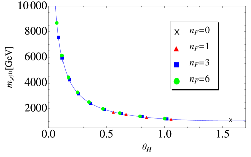
Figure 1: $\theta_{H}$ vs $m_{Z^{(1)}}$ for $m_{H}=126\,$GeV with $n_{F}$ degenerate dark fermions.

Similarly the Higgs cubic and quartic self-couplings, $\lambda_{3}$ and $\lambda_{4}$ are plotted against $\theta_{H}$ for $n_{F}=0,1,3,9$ in Fig. 2. The fitting curves are given by

$$\hskip-28.45274pt\lambda_{3}/{\rm GeV}=26.7\cos\theta_{H}+1.42(1+\cos 2\theta_{H})~{},$$ (3.17)

$$\hskip-28.45274pt\lambda_{4}=-0.0106+0.0304\cos 2\theta_{H}+0.00159\cos 4\theta_{H}~{}.$$ (3.18)

These numbers should be compared with $\lambda_{3}^{\rm SM}=31.5\,$GeV and $\lambda_{4}^{\rm SM}=0.0320$ in the SM. We note that the effective potential $V_{\rm eff}(\theta_{H})$ is bounded from below so that the negative $\lambda_{4}$ for $\theta_{H}>0.6$ does not cause the instability. In the gauge-Higgs unification there is no instability problem in the Higgs couplings.

It should be noted that no universality is found in the mass spectrum of the dark fermions. The mass $m_{F^{(1)}}$ is plotted in Fig. 3 for various $n_{F}$.

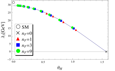
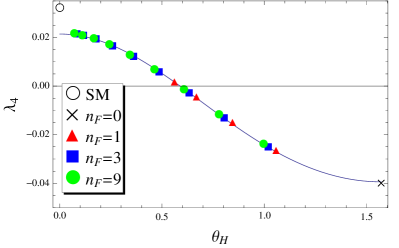
Figure 2: $\theta_{H}$ vs $\lambda_{3}^{H}$ and $\lambda_{4}^{H}$ for $m_{H}=126\,$GeV with $n_{F}$ degenerate dark fermions. In the SM $\lambda_{3}^{\rm SM}=31.5\,$GeV and $\lambda_{4}^{\rm SM}=0.0320$. The fitting curves are given by (3.18).

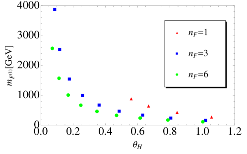
Figure 3: $\theta_{H}$ vs $m_{F}$ for $m_{H}=126\,$GeV with $n_{F}$ degenerate dark fermions.

The universality relations are determined with the fixed Higgs boson mass $m_{H}$. If $m_{H}$ were smaller or larger than the observed value, the universality relations would slightly change. The KK mass scale $m_{\rm KK}$ increases as $m_{H}$. The fitting curve is parmetrized as $m_{\text{KK}}=\alpha/|\sin\theta_{H}|^{\beta}$ with given $m_{H}$. The values of $\alpha$ and $\beta$ for various $m_{H}$ are tabulated in Table 3. We plotted $m_{\rm KK}(\theta_{H})$ for $m_{H}=110,126,140\,$GeV in Fig. 4.

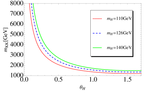
Figure 4: $\theta_{H}$ vs $m_{KK}$ with various values of $m_{H}$.

Table 3: Universality relation $m_{\text{KK}}=\alpha/|\sin\theta_{H}|^{\beta}$ with various value of $m_{H}$.

$m_{H}$(GeV)	$\alpha$(TeV)	$\beta$
110	1.20	0.733
120	1.30	0.766
126	1.35	0.786
130	1.39	0.800
140	1.49	0.820

We stress that the universality leads to powerful predictions. Once the value of $\theta_{H}$ is determined from, say, $m_{Z^{(1)}}$, many other quantities are predicted for experimental confirmation. The gauge-Higgs unification scenario is very predictive.

4 $e^{+}e^{-}$, $\mu^{+}\mu^{-}$ EVENTS IN THE $Z^{\prime}$ SEARCH

One of the distinctive predictions of the $SO(5)\times U(1)$ gauge-Higgs unification is the existence of the KK excited modes of $Z$ and $\gamma$. Independent of the details of the dark fermion sector the universality predicts that $m_{Z^{(1)}},m_{\gamma^{(1)}}\sim 6\,$TeV (3 TeV) for $\theta_{H}=0.1$ (0.2) as depicted in Fig. 1. $Z^{(1)}$ and $\gamma^{(1)}$ partially decay to $e^{+}e^{-}$ or $\mu^{+}\mu^{-}$, which should appear as clear signals in the $Z^{\prime}$ search at LHC[69]-[74]. We evaluate the production and decay rates of those particles.

In our model there are four kinds of neutral gauge bosons at the TeV scale. [See Eq. (2.37]. They are the first KK mode of $Z$ boson, $Z^{(1)}$, the first KK mode of photon, $\gamma^{(1)}$, the $Z_{R}^{(1)}$ boson and the $A^{\hat{4}}$ boson. Among them the $A^{\hat{4}}$ boson does not couple to SM particles so that it escapes from detection in the $Z^{\prime}$ search. $Z^{(1)}$, $\gamma^{(1)}$, and $Z_{R}^{(1)}$ are the candidates for $Z^{\prime}$ bosons.

4.1 Couplings and decay widths

To evaluate the production and decay rates of $Z^{\prime}$ bosons we need to know four-dimensional $Z^{\prime}$ couplings of quarks and leptons. They are obtained from the five-dimensional gauge interaction terms by inserting wave functions of gauge bosons and quarks or leptons and integrating over the fifth-dimensional coordinate. The couplings of the photon, $Z$ boson and $Z_{R}^{(1)}$ boson towers can be written as

$${\cal L}\supset\sum_{n,i}A^{\gamma(n)}_{\mu}\left[g_{u^{i}L}^{\gamma^{(n)}}\bar{u^{i}}^{i}_{L}\gamma^{\mu}u^{i}_{L}+g_{u^{i}R}^{\gamma^{(n)}}\bar{u}^{i}_{R}\gamma^{\mu}u^{i}_{R}+g_{d^{i}L}^{\gamma^{(n)}}\bar{d}^{i}_{L}\gamma^{\mu}d^{i}_{L}+g_{d^{i}R}^{\gamma^{(n)}}\bar{d}^{i}_{R}\gamma^{\mu}d^{i}_{R}\right.$$

$$\left.+g_{e^{i}L}^{\gamma^{(n)}}\bar{e}^{i}_{L}\gamma^{\mu}e^{i}_{L}+g_{e^{i}R}^{\gamma^{(n)}}\bar{e}^{i}_{R}\gamma^{\mu}e^{i}_{R}\right]$$

$$+\sum_{n,i}Z^{(n)}_{\mu}\left[g_{u^{i}L}^{Z^{(n)}}\bar{u}^{i}_{L}\gamma^{\mu}u^{i}_{L}+g_{u^{i}R}^{Z^{(n)}}\bar{u}^{i}_{R}\gamma^{\mu}u^{i}_{R}+g_{d^{i}L}^{Z^{(n)}}\bar{d}^{i}_{L}\gamma^{\mu}d^{i}_{L}+g_{d^{i}R}^{Z^{(n)}}\bar{d}^{i}_{R}\gamma^{\mu}d^{i}_{R}\right.$$

$$\left.+g_{\nu^{i}L}^{Z^{(n)}}\bar{\nu}^{i}_{L}\gamma^{\mu}\nu^{i}_{L}+g_{\nu^{i}R}^{Z^{(n)}}\bar{\nu}^{i}_{R}\gamma^{\mu}\nu^{i}_{R}+g_{e^{i}L}^{Z^{(n)}}\bar{e}^{i}_{L}\gamma^{\mu}e^{i}_{L}+g_{e^{i}R}^{Z^{(n)}}\bar{e}^{i}_{R}\gamma^{\mu}e^{i}_{R}\right]$$

$$+\sum_{n,i}Z^{(n)}_{R\mu}\left[g_{u^{i}L}^{Z_{R}^{(n)}}\bar{u}^{i}_{L}\gamma^{\mu}u^{i}_{L}+g_{u^{i}R}^{Z_{R}^{(n)}}\bar{u}^{i}_{R}\gamma^{\mu}u^{i}_{R}+g_{d^{i}L}^{Z_{R}^{(n)}}\bar{d}^{i}_{L}\gamma^{\mu}d^{i}_{L}+g_{d^{i}R}^{Z_{R}^{(n)}}\bar{d}^{i}_{R}\gamma^{\mu}d^{i}_{R}\right.$$

$$\left.+g_{\nu^{i}L}^{Z_{R}^{(n)}}\bar{\nu}^{i}_{L}\gamma^{\mu}\nu^{i}_{L}+g_{\nu^{i}R}^{Z_{R}^{(n)}}\bar{\nu}^{i}_{R}\gamma^{\mu}\nu^{i}_{R}+g_{e^{i}L}^{Z_{R}^{(n)}}\bar{e}^{i}_{L}\gamma^{\mu}e^{i}_{L}+g_{e^{i}R}^{Z_{R}^{(n)}}\bar{e}^{i}_{R}\gamma^{\mu}e^{i}_{R}\right]$$ (4.1)

where the superscript $i$ denotes the generation, i.e., $(u^{1},u^{2},u^{3})=(u,c,t)$, etc. Explicit formulas for the gauge couplings are given in Appendix D. The relevant couplings of the $Z^{\prime}$ bosons are tabulated in Table 4 and Table 5.

Table 4: Masses, total decay widths and couplings of the $Z^{\prime}$ bosons to SM particles in the first generation for $\theta_{H}=0.114$. Couplings to $\mu$ are approximately the same as those to $e$.

$Z^{\prime}$	$m$(TeV)	$\Gamma$(GeV)	$g_{uL}^{Z^{\prime}}$	$g_{dL}^{Z^{\prime}}$	$g_{eL}^{Z^{\prime}}$	$g_{uR}^{Z^{\prime}}$	$g_{dR}^{Z^{\prime}}$	$g_{eR}^{Z^{\prime}}$
$Z$	0.0912	2.44	0.257	$-$0.314	$-$0.200	$-$0.115	0.0573	0.172
$Z_{R}^{(1)}$	5.73	482	0	0	0	0.641	$-$0.321	$-$0.978
$Z^{(1)}$	6.07	342	$-$0.0887	0.108	0.0690	$-$0.466	0.233	0.711
$\gamma^{(1)}$	6.08	886	$-$0.0724	0.0362	0.109	0.846	$-$0.423	$-$1.29
$Z^{(2)}$	9.14	1.29	$-$0.00727	0.00889	0.00565	$-$0.00548	0.00274	0.00856

Table 5: Masses, total decay widths and couplings of the $Z^{\prime}$ bosons to SM particles in the first generation for $\theta_{H}=0.073$.

$Z^{\prime}$	$m$(TeV)	$\Gamma$(GeV)	$g_{uL}^{Z^{\prime}}$	$g_{dL}^{Z^{\prime}}$	$g_{eL}^{Z^{\prime}}$	$g_{uR}^{Z^{\prime}}$	$g_{dR}^{Z^{\prime}}$	$g_{eR}^{Z^{\prime}}$
$Z_{R}^{(1)}$	8.00	553	0	0	0	0.588	$-$0.294	$-$0.896
$Z^{(1)}$	8.61	494	$-$0.100	0.123	0.0780	$-$0.426	0.213	0.650
$\gamma^{(1)}$	8.61	1.04$\times 10^{3}$	$-$0.0817	0.0408	0.123	0.775	$-$0.388	$-$1.18

The decay width of the $Z^{\prime}$ boson is given by

$$\Gamma_{Z^{\prime}}=\sum_{i}\frac{m_{Z^{\prime}}}{12\pi}\left(\frac{\left(g_{iL}^{Z^{\prime}}\right)^{2}+\left(g_{iR}^{Z^{\prime}}\right)^{2}}{2}+2g_{iL}^{Z^{\prime}}g_{iR}^{Z^{\prime}}\frac{m_{i}^{2}}{m_{Z^{\prime}}^{2}}\right)\sqrt{1-\frac{4m_{i}^{2}}{m_{Z^{\prime}}^{2}}}~{}.$$ (4.2)

Here $i$ runs over all fermions including SM fermions and dark fermions. The contribution of its decay to $W^{+}W^{-}$ is very small and can be neglected[59]. The evaluated $\Gamma_{Z^{\prime}}$ for $\theta_{H}=0.114$ is summarized in Table 4. It is seen that all of $Z_{R}^{(1)}$, $Z^{(1)}$, and $\gamma^{(1)}$ have large decay widths ($300\sim 900$ GeV) in quite contrast to the narrow width of the $Z$ boson. It is mainly due to the large couplings of right-handed quarks and leptons.

4.2 Production at LHC

In our study, we calculate the dilepton production cross sections through the $Z^{\prime}$ boson exchange together with the SM processes mediated by the $Z$ boson and photon. The dependence of the cross section on the final state dilepton invariant mass $M_{\ell\ell}$ is described as

$$\frac{d\sigma(pp\to\ell^{+}\ell^{-}X)}{dM_{\ell\ell}} = \sum_{q}\int^{1}_{-1}d\cos\theta\int^{1}_{\frac{M_{\ell\ell}^{2}}{E_{\rm CMS}^{2}}}dx_{1}\frac{2M_{\ell\ell}}{x_{1}E_{\rm CMS}^{2}}$$ (4.3)

$$\times f_{q}(x_{1},M_{\ell\ell}^{2})f_{\bar{q}}\left(\frac{M_{\ell\ell}^{2}}{x_{1}E_{\rm CMS}^{2}},M_{\ell\ell}^{2}\right)\frac{d\sigma(\bar{q}q\to\ell^{+}\ell^{-})}{d\cos\theta},$$

where $E_{\rm CMS}$ is the center-of-mass energy of the LHC and $f_{q}$’s are the parton distribution functions(PDFs) for $q$ quark. In our numerical analysis, we employ CTEQ5M [75] for the PDFs. Formulas to calculate $d\sigma(\bar{q}q\to\ell^{+}\ell^{-})/d\cos\theta$ are listed in Appendix E.

Figure 5 shows the differential cross section for $pp\to\mu^{+}\mu^{-}$ together with the SM cross section mediated by the $Z$ boson and photon for $\theta_{H}=0.114$ ($n_{F}=5$, $z_{L}=10^{5}$). The deviation from the SM is very small below 3 TeV because the couplings of the $Z$ boson or photon to SM fermions are almost the same as in the SM. For this reason it is difficult to see the signals of the gauge-Higgs unification at 8 TeV LHC experiments. In the case of $\theta_{H}=0.251$ ($n_{F}=5$, $z_{L}=10^{7}$), the deviation from the SM is large. The $Z^{\prime}$ masses are around 3 TeV (See Table 1.) and the decay widths of $Z_{R}^{(1)}$ ,$Z^{(1)}$ and $\gamma^{(1)}$ are 341, 221 and 629 GeV. The masses of $Z^{\prime}$ bosons are heavier than the plot range of Fig. 5. However the decay widths of $Z^{\prime}$ bosons are very wide and the deviation from the SM is large. Therefore the $\theta_{H}=0.251$ case is excluded by the 8 TeV LHC experiments.

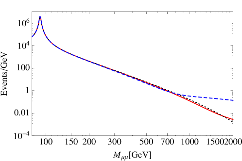
Figure 5: The differential cross section multiplied by an integrated luminosity of 20.6 fb^-1 for $pp\to\mu^{+}\mu^{-}X$ at the 8 TeV LHC for $\theta_{H}=0.114$ (red solid curve) and for $\theta_{H}=0.251$ (blue dashed curve). The black dashed line represents the SM background.

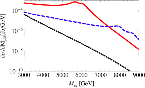
Figure 6: The differential cross section for $pp\to\mu^{+}\mu^{-}X$ at the 14 TeV LHC for $\theta_{H}=0.114$ (red solid curve) and for $\theta_{H}=0.073$ (blue dashed curve) . The nearly straight line represents the SM background.

On the other hand, at 14 TeV LHC experiments, we expect the signals. Figure 6 shows the differential cross section $d\sigma/dM_{\mu\mu}$ in the range $3\,{\rm TeV}<M_{\mu\mu}<9\,$TeV for $\theta_{H}=0.114$ and 0.073. The contributions from $Z^{(2)}$ boson and higher KK modes are negligible because the couplings are very small and the widths are very narrow (see Table 4). One sees a very large deviation from the SM, which can be detected at the upgraded LHC.

5 CONCLUSIONS

In the present paper we have explored LHC signals of the $SO(5)\times U(1)$ gauge-Higgs unification, particularly dilepton events associated with the production and decay of the $Z^{\prime}$ bosons at 14 TeV LHC. In the $SO(5)\times U(1)$ gauge-Higgs unification the four-dimensional Higgs boson appears as a part of the extra-dimensional component of the $SO(5)$ gauge fields, and the quark or lepton multiplets are introduced in the vector representation of $SO(5)$. In addition, dark fermions are introduced in the spinor representation of $SO(5)$, which are vital to realize the observed unstable Higgs boson.

The four-dimensional Higgs boson is the fluctuation mode of the Aharonov-Bohm phase $\theta_{H}$ in the fifth dimension. The phase $\theta_{H}$, determined by the location of the global minimum of the effective potential $V_{\rm eff}(\theta_{H})$, plays an important role in determining the couplings among gauge boson, quarks and leptons, and the Higgs boson. It has been known that the value $\theta_{H}<0.2$ is consistent with the data at low energies.

The shape of $V_{\rm eff}(\theta_{H})$, and therefore the location of global minimum $\theta_{H}$, sensitively depends on the details of the dark fermion sector, which could spoil the predictability of the gauge-Higgs unification scenario. On the contrary, we have shown that there holds the universality in the relations among $m_{\rm KK}$, $m_{Z^{(1)}}$, $m_{\gamma^{(1)}}$, $m_{Z_{R}^{(1)}}$, $\lambda_{3}$, $\lambda_{4}$ and $\theta_{H}$, irrespective of the details of the dark fermion sector. For instance, one finds that $m_{Z^{(1)}}(\theta_{H})\sim 1044\,{\rm GeV}/(\sin\theta_{H})^{0.804}$. The universality implies that once the value of, say, $m_{Z^{(1)}}$ is determined from experiments, then other quantities such as $\lambda_{3}$ and $\lambda_{4}$ are predicted to be tested.

In the $SO(5)\times U(1)$ gauge-Higgs unification the three gauge bosons, $Z_{R}^{(1)}$, $Z^{(1)}$, and $\gamma^{(1)}$, appear as $Z^{\prime}$ bosons in dilepton events at LHC. It is interesting that the masses of these bosons turn out around 6 (8 TeV) for $\theta_{H}=0.114$ ($0.073$), which is exactly in the region explored at the 14 TeV LHC. As right-handed quarks and leptons have large couplings to those $Z^{\prime}$ bosons, the widths of those bosons become large; the decay widths of $Z_{R}^{(1)}$, $Z^{(1)}$ and $\gamma^{(1)}$ are 482, 342 and 886 GeV (553, 494 GeV and 1.04 TeV) for $\theta_{H}=0.114$ (0.073). Notice the relatively large ratio of ${\rm width}/{\rm mass}=0.06\sim 0.15$ in contrast to that of the $Z$ boson. As the difference in masses of $Z^{(1)}$ and $\gamma^{(1)}$ is small, there should appear two peaks in dilepton events. Due to the large widths the excess of events over those expected in the SM should be seen in much wider range of energies. For $\theta_{H}=0.114$, for instance, an excess due to the broad widths of the $Z^{\prime}$ resonances should be observed above 3 TeV in the dilepton invariant mass. The discovery of the $Z^{\prime}$ bosons in the 3 - 9 TeV range would give strong support for the gauge-Higgs unification, signaling the existence of extra dimensions.

In the present paper we have focused on the LHC signals classified in the universality class, specifically on the $Z^{\prime}$ events. There are other collider signals [76]-[81] such as the forward-backward asymmetry (at Tevatron) and the charge asymmetry (at LHC) in $t\bar{t}$ pair production and QCD parity violation at LHC[82]-[86]. We hope to report on these issues in the near future.

Acknowledgements

This work was supported in part by JSPS KAKENHI GRANTS, No. 23104009 (Y.H. and Y.O.), No. 21244036 (Y.H.) and No. 2518610 (T.S.). H.H. is supported by NRF Research Grant 2012R1A2A1A01006053 (HH) of the Republic of Korea.

Appendix A BASE FUNCTIONS

Mode functions for KK towers are expressed in terms of Bessel functions. For gauge fields we define

$$\hskip-28.45274ptC(z;\lambda)=\frac{\pi}{2}\lambda zz_{L}F_{1,0}(\lambda z,\lambda z_{L})~{},\quad C^{\prime}(z;\lambda)=\frac{\pi}{2}\lambda^{2}zz_{L}F_{0,0}(\lambda z,\lambda z_{L})~{},$$ (A.1)

$$\hskip-28.45274ptS(z;\lambda)=-\frac{\pi}{2}\lambda zF_{1,1}(\lambda z,\lambda z_{L})~{},\quad S^{\prime}(z;\lambda)=-\frac{\pi}{2}\lambda^{2}zF_{0,1}(\lambda z,\lambda z_{L})~{},$$ (A.2)

$$\hskip-28.45274pt\hat{S}(z;\lambda)=\frac{C(1;\lambda)}{S(1;\lambda)}\,S(z;\lambda)~{},$$ (A.3)

$$\hskip-28.45274ptF_{\alpha,\beta}(u,v)=J_{\alpha}(u)Y_{\beta}(v)-Y_{\alpha}(u)J_{\beta}(v)~{}.$$ (A.4)

These functions satisfy

$$\hskip-28.45274ptC(z_{L};\lambda)=z_{L}~{},~{}~{}C^{\prime}(z_{L};\lambda)=0~{},~{}~{}S(z_{L};\lambda)=0~{},~{}~{}S^{\prime}(z_{L};\lambda)=\lambda~{},$$ (A.5)

$$\hskip-28.45274ptCS^{\prime}-SC^{\prime}=\lambda z~{}.$$ (A.6)

For fermions with a bulk mass parameter $c$ we define

$$\hskip-28.45274pt\begin{pmatrix}C_{L}\cr S_{L}\end{pmatrix}(z;\lambda,c)=\pm\frac{\pi}{2}\lambda\sqrt{zz_{L}}F_{c+{1\over 2},c\mp{1\over 2}}(\lambda z,\lambda z_{L})~{},$$ (A.7)

$$\hskip-28.45274pt\begin{pmatrix}C_{R}\cr S_{R}\end{pmatrix}(z;\lambda,c)=\mp\frac{\pi}{2}\lambda\sqrt{zz_{L}}F_{c-{1\over 2},c\pm{1\over 2}}(\lambda z,\lambda z_{L})~{}.$$ (A.8)

They satisfy

$$\hskip-28.45274ptD_{+}(c)\begin{pmatrix}C_{L}\cr S_{L}\end{pmatrix}=\lambda\begin{pmatrix}S_{R}\cr C_{R}\end{pmatrix},~{}~{}D_{-}(c)\begin{pmatrix}C_{R}\cr S_{R}\end{pmatrix}=\lambda\begin{pmatrix}S_{L}\cr C_{L}\end{pmatrix},$$ (A.9)

$$\hskip-28.45274ptD_{\pm}(c)=\pm\frac{d}{dz}+\frac{c}{z}~{},$$ (A.10)

and

$$\hskip-28.45274ptC_{R}=C_{L}=1~{},~{}~{}S_{R}=S_{L}=0~{}~{}~{}{\rm for~{}}z=z_{L}~{},$$ (A.11)

$$\hskip-28.45274ptC_{L}C_{R}-S_{L}S_{R}=1~{},~{}~{}S_{L}(z;\lambda,-c)=-S_{R}(z;\lambda,c)~{}.$$ (A.12)

Appendix B KK TOWERS OF BOSONIC FIELDS

B.1 Twisted gauge

To find the spectrum and wave function of each KK mode for $\theta_{H}\not=0$, it is convenient to move to the twisted gauge in which $\raise 0.68889pt\hbox{$\langle$}\lower 0.68889pt\hbox{}\tilde{A}_{z}\raise 0.68889pt\hbox{$\rangle$}\lower 0.68889pt\hbox{}=0$. This is achieved by a gauge transformation $\tilde{A}_{M}=\Omega A_{M}\Omega^{-1}+1/g_{A}\Omega\partial_{M}\Omega^{-1}$ with $\partial_{z}\Omega=-ig_{A}\Omega\raise 0.68889pt\hbox{$\langle$}\lower 0.68889pt\hbox{}A_{z}\raise 0.68889pt\hbox{$\rangle$}\lower 0.68889pt\hbox{}$;

$$\hskip-28.45274pt\Omega=\exp\left\{ig_{A}\theta_{H}f_{H}T^{\hat{4}}\int^{L}_{y}dy\,u_{H}(y)\right\}$$ (B.1)

$$\hskip-17.07182pt=\exp\left\{i\theta_{H}\frac{z_{L}^{2}-z^{2}}{z_{L}^{2}-1}\sqrt{2}\,T^{\hat{4}}\right\}\quad\text{for }1\leq z\leq z_{L}~{}.$$ (B.2)

The orbifold boundary condition matrices $P_{j}$ at $y=y_{j}$ [$(y_{0},y_{1})=(0,L)$] change from $P_{j}$ to $\tilde{P}_{j}=\Omega(y_{j}-y)P_{0}\Omega(y_{j}+y)^{-1}$. $\Omega$ in (B.2) has been chosen such that $\Omega|_{y=L}=1$ and the orbifold boundary condition at the TeV brane remains unchanged. On the other hand, the orbifold boundary condition matrix $P_{0}$ changes to $\tilde{P}_{0}=\Omega(-y)P_{0}\Omega(y)^{-1}$;

$$\hskip-28.45274pt\tilde{P}_{0}^{{\rm vec}}=\begin{pmatrix}-1&&&&\\ &-1&&&\\ &&-1&&\\ &&&-\cos 2\theta_{H}&\sin 2\theta_{H}\\ &&&\sin 2\theta_{H}&\cos 2\theta_{H}\end{pmatrix},$$ (B.3)

$$\hskip-28.45274pt\tilde{P}_{0}^{{\rm sp}}=\begin{pmatrix}\cos\theta_{H}&-i\sin\theta_{H}\cr i\sin\theta_{H}&-\cos\theta_{H}\end{pmatrix}\otimes I_{2}~{}~{}.$$ (B.4)

In the twisted gauge the fields satisfy free equations at the tree level, but obey the $\theta_{H}$-dependent boundary condition specified by (B.4). Wave functions of the four-dimensional components of the gauge fields are expressed in terms of either $C(z;\lambda)$ or $S(z;\lambda)$ in (A.4), depending on the boundary condition (Neumann or Dirichelet) at the TeV brane. Wave functions of the fifth-dimensional components of the gauge fields, on the other hand, are expressed in terms of either $C^{\prime}(z;\lambda)$ or $S^{\prime}(z;\lambda)$. The boundary condition at the Planck brane at $z=1$ mixes fields through (B.4) and determines eigenvalues $\{\lambda_{n}\}$ in each KK tower.

B.2 KK towers of $A_{\mu}$ and $B_{\mu}$

$A_{\mu}(x,z)$ and $B_{\mu}^{X}(x,z)$ are expanded in KK towers.

$$\tilde{A}_{\mu}(x,z)+\frac{g_{B}}{g_{A}}B_{\mu}(x,z)T_{B}$$

$$\hskip 0.0pt=\hat{W}_{\mu}^{-}+\hat{W}_{\mu}^{+}+\hat{Z}_{\mu}+\hat{A}_{\mu}^{\gamma}+\hat{W}_{R\mu}^{-}+\hat{W}_{R\mu}^{+}+\hat{Z}_{R\mu}+\hat{A}_{\mu}^{\hat{4}}~{},$$ (B.5)

where

$$\hskip-28.45274pt\hat{W}_{\mu}^{\mp}=\sum_{n}W_{\mu}^{(n)\mp}(x)\left\{h_{W^{(n)}}^{L}\frac{T^{1_{L}}\mp iT^{2_{L}}}{\sqrt{2}}+h_{W^{(n)}}^{R}\frac{T^{1_{R}}\mp iT^{2_{R}}}{\sqrt{2}}+\hat{h}_{W^{(n)}}\frac{T^{\hat{1}}\mp iT^{\hat{2}}}{\sqrt{2}}\right\},$$

$$\hskip-28.45274pt\hat{Z}_{\mu}=\sum_{n}Z_{\mu}^{(n)}(x)\left\{h_{Z^{(n)}}^{L}T^{3_{L}}+h_{Z^{(n)}}^{R}T^{3_{R}}+\hat{h}_{Z^{(n)}}T^{\hat{3}}+\frac{g_{B}}{g_{A}}h_{Z^{(n)}}^{B}T_{B}\right\},$$

$$\hskip-28.45274pt\hat{A}^{\gamma}_{\mu}=\sum_{n}A^{\gamma(n)}_{\mu}(x)\left\{h_{\gamma^{(n)}}^{L}T^{3_{L}}+h_{\gamma^{(n)}}^{R}T^{3_{R}}+\frac{g_{B}}{g_{A}}h_{\gamma^{(n)}}^{B}T_{B}\right\},$$

$$\hskip-28.45274pt\hat{W}_{R\mu}^{\mp}=\sum_{n}W_{R\mu}^{(n)\mp}(x)\left\{h_{W_{R}^{(n)}}^{L}\frac{T^{1_{L}}\mp iT^{2_{L}}}{\sqrt{2}}+h_{W_{R}^{(n)}}^{R}\frac{T^{1_{R}}\mp iT^{2_{R}}}{\sqrt{2}}\right\},$$

$$\hskip-28.45274pt\hat{Z}_{R\mu}=\sum_{n}Z_{R\mu}^{(n)}(x)\left\{h_{Z_{R}^{(n)}}^{L}T^{3_{L}}+h_{Z_{R}^{(n)}}^{R}T^{3_{R}}+\frac{g_{B}}{g_{A}}h_{Z_{R}^{(n)}}^{B}T_{B}\right\},$$

$$\hskip-28.45274pt\hat{A}^{\hat{4}}_{\mu}=\sum_{n}A^{\hat{4}(n)}_{\mu}(x)\hat{h}_{A^{\hat{4}(n)}}T^{\hat{4}},$$ (B.6)

$$\hskip 0.0pt\hat{W}^{\pm}=\frac{\hat{W}^{1}\mp i\hat{W}^{2}}{\sqrt{2}}~{},\quad\hat{W}_{R}^{\pm}=\frac{\hat{W}_{R}^{1}\mp i\hat{W}_{R}^{2}}{\sqrt{2}}~{}.$$ (B.7)

The two gauge coupling constants are related to the weak mixing angle $\theta_{W}$ by

$$c_{\phi}=\frac{g_{A}}{\sqrt{g_{A}^{2}+g_{B}^{2}}}~{},~{}~{}s_{\phi}=\frac{g_{B}}{\sqrt{g_{A}^{2}+g_{B}^{2}}}~{},~{}~{}\cos\theta_{W}=\frac{1}{\sqrt{1+s_{\phi}^{2}}}~{}.$$ (B.8)

The KK spectrum and corresponding wave functions for each tower are summarized as follows.

$W$ tower

The spectrum of the $W$ tower is given by

$$2S(1;\lambda_{W^{(n)}})C^{\prime}(1;\lambda_{W^{(n)}})+\lambda_{W^{(n)}}\sin^{2}\theta_{H}=0~{}.$$ (B.9)

which includes the $W$ boson as the lowest mode $W=W^{(0)}$. The mode functions are

$$\hskip-28.45274pt\begin{pmatrix}h_{W^{(n)}}^{L}(z)\\ h_{W^{(n)}}^{R}(z)\\ \hat{h}_{W^{(n)}}(z)\end{pmatrix}=\frac{1}{\sqrt{2\,r_{W^{(n)}}}}\begin{pmatrix}(1+\cos\theta_{H})C(z;\lambda_{W^{(n)}})\\ (1-\cos\theta_{H})C(z;\lambda_{W^{(n)}})\\ -\sqrt{2}\sin\theta_{H}\hat{S}(z;\lambda_{W^{(n)}})\end{pmatrix},$$

$$\hskip-28.45274ptr_{W^{(n)}}=\int_{1}^{z_{L}}\frac{dz}{kz}\left\{(1+\cos^{2}\theta_{H})C(z;\lambda_{W^{(n)}})^{2}+\sin^{2}\theta_{H}\hat{S}(z;\lambda_{W^{(n)}})^{2}\right\}.$$ (B.10)

$Z$ tower

KK spectrum of the $Z$ tower is given by

$$2S(1;\lambda_{Z^{(n)}})C^{\prime}(1;\lambda_{Z^{(n)}})+(1+s_{\phi}^{2})\lambda_{Z^{(n)}}\sin^{2}\theta_{H}=0~{},$$ (B.11)

which includes the $Z$ boson $Z=Z^{(0)}$. The mode functions of the $Z$ tower are

$$\hskip-28.45274pt\begin{pmatrix}h_{Z^{(n)}}^{L}(z)\\ \kern 3.0pt\cr h_{Z^{(n)}}^{R}(z)\\ \kern 3.0pt\cr\hat{h}_{Z^{(n)}}(z)\\ \kern 3.0pt\cr h_{Z^{(n)}}^{B}\end{pmatrix}=\frac{1}{\sqrt{1+s_{\phi}^{2}}}\frac{1}{\sqrt{2\,r_{Z^{(n)}}}}\begin{pmatrix}\big{\{}(1+s_{\phi}^{2})(1+\cos\theta_{H})-2s_{\phi}^{2}\big{\}}C(z;\lambda_{Z^{(n)}})\\ \kern 3.0pt\cr\big{\{}(1+s_{\phi}^{2})(1-\cos\theta_{H})-2s_{\phi}^{2}\big{\}}C(z;\lambda_{Z^{(n)}})\\ \kern 3.0pt\cr-\sqrt{2}(1+s_{\phi}^{2})\sin\theta_{H}\hat{S}(z;\lambda_{Z^{(n)}})\\ \kern 3.0pt\cr-2s_{\phi}c_{\phi}C(z;\lambda_{Z^{(n)}})\end{pmatrix},$$

$$\hskip-28.45274ptr_{Z^{(n)}}=\int_{1}^{z_{L}}\frac{dz}{kz}\biggl{\{}c_{\phi}^{2}C(z;\lambda_{Z^{(n)}})^{2}$$

$$\phantom{MM}+(1+s_{\phi}^{2})[\cos^{2}\theta_{H}C(z;\lambda_{Z^{(n)}})^{2}+\sin^{2}\theta_{H}\hat{S}(z;\lambda_{Z^{(n)}})^{2}\biggr{\}}.$$ (B.12)

Photon tower

The spectrum of the photon tower is given by

$$C^{\prime}(1;\lambda_{\gamma^{(n)}})=0~{},$$ (B.13)

which includes a massless photon $\lambda_{\gamma^{(0)}}=0$. The mode functions are

$$\hskip-28.45274pt\begin{pmatrix}h_{\gamma^{(n)}}^{L}(z)\\ h_{\gamma^{(n)}}^{R}(z)\\ h_{\gamma^{(n)}}^{B}\end{pmatrix}=\frac{1}{\sqrt{1+s_{\phi}^{2}}}\frac{1}{\sqrt{r_{\gamma^{(n)}}}}\begin{pmatrix}s_{\phi}C(z;\lambda_{\gamma^{(n)}})\\ s_{\phi}C(z;\lambda_{\gamma^{(n)}})\\ c_{\phi}\end{pmatrix}C(z;\lambda_{\gamma^{(n)}}),$$

$$\hskip 0.0ptr_{\gamma^{(n)}}=\int_{1}^{z_{L}}\frac{dz}{kz}C(z;\lambda_{\gamma^{(n)}})^{2}.$$ (B.14)

In particular for the photon $\gamma=\gamma^{(0)}$,

$$\begin{pmatrix}h_{\gamma}^{L}(z)\\ h_{\gamma}^{R}(z)\\ h_{\gamma}^{B}\end{pmatrix} = \frac{1}{\sqrt{(1+s_{\phi}^{2})L}}\begin{pmatrix}s_{\phi}\\ s_{\phi}\\ c_{\phi}\end{pmatrix}.$$ (B.15)

$W_{R}$ tower

The spectrum of the $W_{R}$ tower is given by

$$C(1;\lambda_{W_{R}^{(n)}})=0~{},$$ (B.16)

The corresponding mode functions are

$$\hskip-28.45274pt\begin{pmatrix}h_{W_{R}^{(n)}}^{L}(z)\\ h_{W_{R}^{(n)}}^{R}(z)\end{pmatrix}=\frac{1}{\sqrt{2\,r_{W_{R}^{(n)}}}}\begin{pmatrix}+1-\cos\theta_{H}\\ -1-\cos\theta_{H}\end{pmatrix}C(z;\lambda_{W_{R}^{(n)}})~{},$$

$$\hskip 0.0ptr_{W_{R}^{(n)}}=\int_{1}^{z_{L}}\frac{dz}{kz}C(z;\lambda_{W_{R}^{(n)}})^{2}~{}.$$ (B.17)

$Z_{R}$ tower

The spectrum of the $Z_{R}$ tower is given by

$$C(1;\lambda_{Z_{R}^{(n)}})=0~{},$$ (B.18)

turning out identical to the $W_{R}$ tower spectrum, $\lambda_{Z_{R}^{(n)}}=\lambda_{W_{R}^{(n)}}$. The corresponding mode functions are

$$\hskip-28.45274pt\begin{pmatrix}h_{Z_{R}^{(n)}}^{L}(z)\\ h_{Z_{R}^{(n)}}^{R}(z)\\ h_{Z_{R}^{(n)}}^{B}\end{pmatrix}=\frac{1}{\sqrt{1+(1+2t_{\phi}^{2})\cos^{2}\theta_{H}}\sqrt{2\,r_{Z_{R}^{(n)}}}}\begin{pmatrix}-\cos\theta_{H}-1\\ -\cos\theta_{H}+1\\ 2t_{\phi}\cos\theta_{H}\end{pmatrix}C(z;\lambda_{Z_{R}^{(n)}})~{},$$

$$\hskip 0.0ptr_{Z_{R}^{(n)}}=\int_{1}^{z_{L}}\frac{dz}{kz}C(z;\lambda_{Z_{R}^{(n)}})^{2}=r_{W_{R}^{(n)}},\quad t_{\phi}\equiv\frac{s_{\phi}}{c_{\phi}}~{}.$$ (B.19)

$A^{\hat{4}}$ tower

The spectrum and wave functions of $A^{\hat{4}}$ tower are

$$\hskip-28.45274ptS(1;\lambda_{A^{\hat{4}(n)}})=0~{},$$ (B.20)

$$\hskip-28.45274pth_{A^{\hat{4}(n)}}(z)=\frac{1}{\sqrt{r_{A^{\hat{4}(n)}}}}S(z;\lambda_{A^{\hat{4}(n)}}),\quad r_{A^{\hat{4}(n)}}=\int_{1}^{z_{L}}\frac{dz}{kz}S(z;\lambda_{A^{\hat{4}(n)}})^{2}~{}.$$ (B.21)

B.3 KK towers of $A_{z}$ and $B_{z}$

$A_{z}(x,z)$ and $B_{z}(x,z)$ are expanded in KK towers as

$$\tilde{A}_{z}(x,z) = \sum_{a=1}^{3}\hat{G}^{a}+\sum_{a=1}^{3}\hat{D}^{a}+\hat{H},$$

$$\hat{G}^{a} = \sum_{n}G^{a(n)}(x)\left\{u_{G^{(n)}}^{L}T^{a_{L}}+u_{G^{(n)}}^{R}T^{a_{R}}\right\},$$

$$\hat{D}^{a} = \sum_{n}D^{a(n)}(x)\left\{u_{D^{(n)}}^{L}T^{a_{L}}+u_{D^{(n)}}^{R}T^{a_{R}}+\hat{u}_{D^{(n)}}T^{\hat{a}}\right\},$$

$$\hat{H} = \sum_{n}H^{(n)}(x)u_{H^{(n)}}T^{\hat{4}},$$

$${B}_{z}(x,z) = \sum_{n}B^{(n)}(x)u_{B^{(n)}}T_{B}~{}.$$ (B.22)

$G$ tower

The $G$ tower spectrum and corresponding mode functions are given by

$$C^{\prime}(1;\lambda_{G^{(n)}}) = 0,\quad\lambda_{G^{(n)}}\neq 0.$$ (B.23)

$$u_{G^{(n)}}^{L}=u_{G^{(n)}}^{R} = \frac{1}{\sqrt{2}}\frac{1}{\sqrt{r_{G^{(n)}}}}C^{\prime}(z;\lambda_{G^{(n)}}),$$

$$r_{G^{(n)}} = \int_{1}^{z_{L}}\frac{kdz}{z}C^{\prime}(z;\lambda_{G^{(n)}})^{2}.$$ (B.24)

$D$ tower

The spectrum of the $D$ tower is given by

$$\hskip-28.45274ptS(1;\lambda_{D^{(n)}})C^{\prime}(1;\lambda_{D^{(n)}})+\lambda_{D^{(n)}}\sin^{2}\theta_{H}$$ (B.25)

$$\hskip-28.45274pt=C(1;\lambda_{D^{(n)}})S^{\prime}(1;\lambda_{D^{(n)}})-\lambda_{D^{(n)}}\cos^{2}\theta_{H}=0~{}.$$ (B.26)

Corresponding mode functions are given by

$$\hskip-28.45274pt\begin{pmatrix}h_{D^{(n)}}^{L}(z)\\ h_{D^{(n)}}^{R}(z)\\ \hat{h}_{D^{(n)}}(z)\end{pmatrix}=\frac{1}{\sqrt{2\,r_{D^{(n)}}}}\begin{pmatrix}\cos\theta_{H}C^{\prime}(z;\lambda_{D^{(n)}})\\ -\cos\theta_{H}C^{\prime}(z;\lambda_{D^{(n)}})\\ -\sqrt{2}\sin\theta_{H}\hat{S}^{\prime}(z;\lambda_{D^{(n)}})\end{pmatrix},\quad\hat{S}^{\prime}(z;\lambda)=\frac{C(1;\lambda)}{S(1;\lambda)}S^{\prime}(z;\lambda),$$

$$\hskip 0.0ptr_{D^{(n)}}=\int_{1}^{z_{L}}\frac{kdz}{z}\left\{\cos^{2}\theta_{H}C^{\prime}(z;\lambda_{D^{(n)}})^{2}+\sin^{2}\theta_{H}\hat{S}^{\prime}(z;\lambda_{D^{(n)}})^{2}\right\}.$$ (B.27)

Higgs ($H$) tower

The spectrum of the Higgs tower is determined by

$$\lambda_{H^{(n)}}S(1;\lambda_{H^{(n)}}) = 0~{},$$ (B.28)

which includes the zero mode $\lambda_{H^{(0)}}=0$ for the 4D Higgs boson $H=H^{(0)}$. The mode functions are

$$u_{H^{(0)}}(z) = u_{H}(z)=\sqrt{\frac{2}{k(z_{L}^{2}-1)}}~{}z~{},$$ (B.29)

for the 4D Higgs boson, and

$$u_{H^{(n)}}(z) = \frac{1}{\sqrt{r_{H^{(n)}}}}S^{\prime}(z;\lambda_{H^{(n)}}),\quad r_{H^{(n)}}=\int_{1}^{z_{L}}\frac{kdz}{z}S^{\prime}(z;\lambda_{H^{(n)}})^{2}~{},$$ (B.30)

for KK-excited states ($n\geq 1$).

$B$ tower

The $B$ tower spectrum and corresponding mode functions are given by

$$C^{\prime}(1;\lambda_{B^{(n)}}) = 0,\quad\lambda_{B^{(n)}}\neq 0.$$ (B.31)

$$u_{B^{(n)}} = \frac{1}{\sqrt{r_{B^{(n)}}}}C^{\prime}(z;\lambda_{B^{(n)}}),$$

$$r_{B^{(n)}} = \int_{1}^{z_{L}}\frac{kdz}{z}C^{\prime}(z;\lambda_{B^{(n)}})^{2}.$$ (B.32)

Appendix C WAVE FUNCTIONS OF FERMIONS

Wave functions of KK towers of fermions are expressed in terms of $C_{L}(z;\lambda,c)$ and $S_{L}(z;\lambda,c)$ in (A.8) for left-handed components and $C_{R}(z;\lambda,c)$ and $S_{R}(z;\lambda,c)$ for right-handed components.

C.1 Quark-lepton towers

Wave functions for the KK tower of an up-type quark $t$ (top) are given by

$$\hskip-28.45274pt\begin{pmatrix}U_{L}(x,z)\\ B_{L}(x,z)\\ t_{L}(x,z)\\ t^{\prime}_{L}(x,z)\end{pmatrix}\supset\frac{\sqrt{k}z^{2}}{\sqrt{r_{t^{(n)}}}}\begin{pmatrix}a_{U}^{(n)}C_{L}^{(2)}(z,\lambda_{t^{(n)}})\\ \displaystyle a_{B}^{(n)}C_{L}^{(1)}(z,\lambda_{t^{(n)}})\\ a_{t}^{(n)}C_{L}^{(1)}(z,\lambda_{t^{(n)}})\\ a_{t^{\prime}}^{(n)}S_{L}^{(1)}(z,\lambda_{t^{(n)}})\end{pmatrix}t^{(n)}_{L}(x)\equiv\sqrt{k}z^{2}\begin{pmatrix}f^{(n)}_{U_{L}}(z)\\ f^{(n)}_{B_{L}}(z)\\ f^{(n)}_{t_{L}}(z)\\ f^{(n)}_{t^{\prime}_{L}}(z)\end{pmatrix}t^{(n)}_{L}(x)~{},$$ (C.1)

$$\hskip-28.45274pt\begin{pmatrix}U_{R}(x,z)\\ B_{R}(x,z)\\ t_{R}(x,z)\\ t^{\prime}_{R}(x,z)\end{pmatrix}\supset\frac{\sqrt{k}z^{2}}{\sqrt{r_{t^{(n)}}}}\begin{pmatrix}a_{U}^{(n)}S_{R}^{(2)}(z,\lambda_{t^{(n)}})\\ \displaystyle a_{B}^{(n)}S_{R}^{(1)}(z,\lambda_{t^{(n)}})\\ a_{t}^{(n)}S_{R}^{(1)}(z,\lambda_{t^{(n)}})\\ a_{t^{\prime}}^{(n)}C_{R}^{(1)}(z,\lambda_{t^{(n)}})\end{pmatrix}t^{(n)}_{R}(x)\equiv\sqrt{k}z^{2}\begin{pmatrix}f^{(n)}_{U_{R}}(z)\\ f^{(n)}_{B_{R}}(z)\\ f^{(n)}_{t_{R}}(z)\\ f^{(n)}_{t^{\prime}_{R}}(z)\end{pmatrix}t^{(n)}_{R}(x)~{},$$ (C.2)

$$\hskip-17.07182ptr_{t^{(n)}}=\int_{1}^{z_{L}}dz\Big{\{}a_{U}^{(n)2}C_{L}^{(2)}(z,\lambda_{t^{(n)}})^{2}+(a_{B}^{(n)2}+a_{t}^{(n)2})C_{L}^{(1)}(z,\lambda_{t^{(n)}})^{2}+a_{t^{\prime}}^{(n)2}S_{L}^{(1)}(z,\lambda_{t^{(n)}})^{2}\Big{\}}$$ (C.3)

$$\hskip 0.0pt=\int_{1}^{z_{L}}dz\Big{\{}a_{U}^{(n)2}S_{R}^{(2)}(z,\lambda_{t^{(n)}})^{2}+(a_{B}^{(n)2}+a_{t}^{(n)2})S_{R}^{(1)}(z,\lambda_{t^{(n)}})^{2}+a_{t^{\prime}}^{(n)2}C_{R}^{(1)}(z,\lambda_{t^{(n)}})^{2}\Big{\}}.$$

(C.4)

Here $C_{L}^{(i)}(z,\lambda_{t^{(n)}})=C_{L}(z;\lambda_{t^{(n)}},c_{i})$, $S_{R}^{(i)}(z,\lambda_{b^{(n)}})=S_{R}(z;\lambda_{b^{(n)}},c_{i})$, etc., and other towers of $Q_{\rm EM}=\hbox{$\frac{2}{3}$}e$ fermions have been suppressed. The common factors are given by

$$\hskip-28.45274pt\begin{pmatrix}a^{(n)}_{U}\\ a^{(n)}_{B}\\ a^{(n)}_{t}\\ a^{(n)}_{t^{\prime}}\end{pmatrix}=\begin{pmatrix}-\sqrt{2}\tilde{\mu}^{q}C_{L}^{(1)}/\mu_{2}^{q}C_{L}^{(2)}\\ \kern 5.0pt\cr(1-\cos\theta_{H})/\sqrt{2}\\ \kern 5.0pt\cr(1+\cos\theta_{H})/\sqrt{2}\\ \kern 5.0pt\cr-\sin\theta_{H}C_{L}^{(1)}/S_{L}^{(1)}\end{pmatrix},$$ (C.5)

$$\hskip-28.45274ptC_{L}^{(i)}\equiv C_{L}(1;\lambda_{t^{(n)}},c_{i})~{},~{}~{}S_{L}^{(i)}\equiv S_{L}(1;\lambda_{t^{(n)}},c_{i})~{},$$ (C.6)

where $\lambda_{t^{(n)}}$ satisfies

$$\hskip-28.45274pt(\mu_{2}^{q})^{2}C_{L}(1;\lambda_{t^{(n)}},c_{2})\Big{\{}S_{R}(1;\lambda_{t^{(n)}},c_{1})+\frac{\sin^{2}\theta_{H}}{2S_{L}(1;\lambda_{t^{(n)}},c_{1})}\Big{\}}$$ (C.7)

$$\hskip 56.9055pt+(\tilde{\mu}^{q})^{2}C_{L}(1;\lambda_{t^{(n)}},c_{1})S_{R}(1;\lambda_{t^{(n)}},c_{2})=0~{},$$ (C.8)

or for $c_{1}=c_{2}\equiv c_{t}$

$$2\bigg{\{}1+\Big{(}\frac{\mu_{2}^{q}}{\tilde{\mu}^{q}}\Big{)}^{2}\bigg{\}}S_{L}(1;\lambda_{t^{(n)}},c_{t})S_{R}(1;\lambda_{t^{(n)}},c_{t})+\Big{(}\frac{\mu_{2}^{q}}{\tilde{\mu}^{q}}\Big{)}^{2}\sin^{2}\theta_{H}=0~{}.$$ (C.9)

For a down-type quark $b$ (bottom) we have

$$\hskip-28.45274pt\begin{pmatrix}b_{L}(x,z)\\ X_{L}(x,z)\\ D_{L}(x,z)\\ b^{\prime}_{L}(x,z)\end{pmatrix}\supset\frac{\sqrt{k}z^{2}}{\sqrt{r_{b^{(n)}}}}\begin{pmatrix}a^{(n)}_{b}C_{L}^{(1)}(z,\lambda_{b^{(n)}})\\ a^{(n)}_{X}C_{L}^{(2)}(z,\lambda_{b^{(n)}})\\ a^{(n)}_{D}C_{L}^{(2)}(z,\lambda_{b^{(n)}})\\ a^{(n)}_{b^{\prime}}S_{L}^{(2)}(z,\lambda_{b^{(n)}})\end{pmatrix}b^{(n)}_{L}(x)\equiv\sqrt{k}z^{2}\begin{pmatrix}f^{(n)}_{b_{L}}(z)\\ f^{(n)}_{X_{L}}(z)\\ f^{(n)}_{D_{L}}(z)\\ f^{(n)}_{b^{\prime}_{L}}(z)\end{pmatrix}b^{(n)}_{L}(x)~{},$$ (C.10)

$$\hskip-28.45274pt\begin{pmatrix}b_{R}(x,z)\\ X_{R}(x,z)\\ D_{R}(x,z)\\ b^{\prime}_{R}(x,z)\end{pmatrix}\supset\frac{\sqrt{k}z^{2}}{\sqrt{r_{b^{(n)}}}}\begin{pmatrix}a^{(n)}_{b}S_{R}^{(1)}(z,\lambda_{b^{(n)}})\\ a^{(n)}_{X}S_{R}^{(2)}(z,\lambda_{b^{(n)}})\\ a^{(n)}_{D}S_{R}^{(2)}(z,\lambda_{b^{(n)}})\\ a^{(n)}_{b^{\prime}}C_{R}^{(2)}(z,\lambda_{b^{(n)}})\end{pmatrix}b^{(n)}_{R}(x)\equiv\sqrt{k}z^{2}\begin{pmatrix}f^{(n)}_{b_{R}}(z)\\ f^{(n)}_{X_{R}}(z)\\ f^{(n)}_{D_{R}}(z)\\ f^{(n)}_{b^{\prime}_{R}}(z)\end{pmatrix}b^{(n)}_{R}(x)~{},$$ (C.11)

$$\hskip-14.22636pt\begin{pmatrix}a^{(n)}_{b}\\ a^{(n)}_{X}\\ a^{(n)}_{D}\\ a^{(n)}_{b^{\prime}}\end{pmatrix}=\begin{pmatrix}-\sqrt{2}\mu_{2}^{q}C_{L}^{(2)}/\tilde{\mu}^{q}C_{L}^{(1)}\\ \kern 5.0pt\cr(1-\cos\theta_{H})/\sqrt{2}\\ \kern 5.0pt\cr(1+\cos\theta_{H})/\sqrt{2}\\ \kern 5.0pt\cr\sin\theta_{H}C_{L}^{(2)}/S_{L}^{(2)}\end{pmatrix},$$ (C.12)

$$\hskip 0.0ptC_{L}^{(i)}\equiv C_{L}(1;\lambda_{b^{(n)}},c_{i}),\quad S_{L}^{(i)}\equiv S_{L}(1;\lambda_{b^{(n)}},c_{i})~{},$$ (C.13)

$$\hskip-28.45274ptr_{b^{(n)}}=\int_{1}^{z_{L}}dz\Big{\{}a^{(n)2}_{b}C_{L}^{(1)}(z,\lambda_{b^{(n)}})^{2}+(a^{(n)2}_{X}+a^{(n)2}_{D})C_{L}^{(2)}(z,\lambda_{b^{(n)}})^{2}+a^{(n)2}_{b^{\prime}}S_{L}^{(2)}(z,\lambda_{b^{(n)}})^{2}\Big{\}}$$ (C.14)

$$\hskip-17.07182pt=\int_{1}^{z_{L}}dz\Big{\{}a^{(n)2}_{b}S_{R}^{(1)}(z,\lambda_{b^{(n)}})^{2}+(a^{(n)2}_{X}+a^{(n)2}_{D})S_{R}^{(2)}(z,\lambda_{b^{(n)}})^{2}+a^{(n)2}_{b^{\prime}}C_{R}^{(2)}(z,\lambda_{b^{(n)}})^{2}\Big{\}}.$$ (C.15)

The spectrum is determined by

$$\hskip-28.45274pt(\tilde{\mu}^{q})^{2}C_{L}(1;\lambda_{b^{(n)}},c_{1})\left[S_{R}(1;\lambda_{b^{(n)}},c_{2})+\frac{\sin^{2}\theta_{H}}{2S_{L}(1;\lambda_{b^{(n)}},c_{2})}\right]$$ (C.16)

$$\hskip 56.9055pt+(\mu_{2}^{q})^{2}C_{L}(1;\lambda_{b^{(n)}},c_{2})S_{R}(1;\lambda_{b^{(n)}},c_{1})=0~{},$$ (C.17)

or for $c_{1}=c_{2}=c_{t}$

$$2\bigg{\{}1+\Big{(}\frac{\mu_{2}^{q}}{\tilde{\mu}^{q}}\Big{)}^{2}\bigg{\}}S_{L}(1;\lambda_{b^{(n)}},c_{t})S_{R}(1;\lambda_{b^{(n)}},c_{t})+\sin^{2}\theta_{H}=0.$$ (C.18)

For a lepton mupltiplet $(\nu_{\tau},\tau)$, the wave functions are given by the following replacement rules;

$$\hskip-28.45274pt\begin{pmatrix}U\\ B\\ t\\ t^{\prime}\end{pmatrix}\to\begin{pmatrix}\nu_{\tau}\\ L_{2Y}\\ L_{3X}\\ \nu_{\tau}^{\prime}\end{pmatrix},\quad\begin{pmatrix}b\\ D\\ X\\ b^{\prime}\end{pmatrix}\to\begin{pmatrix}L_{3Y}\\ \tau\\ L_{1Y}\\ \tau^{\prime}\end{pmatrix},$$ (C.19)

$$\hskip-28.45274pt(\tilde{\mu}^{q},\mu_{2}^{q})\to(\mu_{3}^{\ell},\tilde{\mu}^{\ell})~{},\quad(\mu_{3}^{q},\mu_{1}^{q})\to(\mu_{1}^{\ell},\mu_{2}^{\ell})~{},$$ (C.20)

$$\hskip-28.45274pt(c_{1},c_{2})\to(c_{4},c_{3})~{}.$$ (C.21)

C.2 Dark fermions ($SO(5)$-spinor fermions)

The spectrum of the KK tower of the dark fermion $\Psi_{F_{i}}$ is determined by

$$C_{L}(1;\lambda_{i,n},c_{F_{i}})C_{R}(1;\lambda_{i,n},c_{F_{i}})-\sin^{2}\frac{\theta_{H}}{2}=0~{}.$$ (C.22)

Its KK expansion is given by

$$\hskip-28.45274pt\Psi_{F_{i},R}(x,z)=\sqrt{k}z^{2}\sum_{n=1}^{\infty}\left\{\begin{pmatrix}f_{i,lR}^{(n)}(z)\cr 0\cr f_{i,rR}^{(n)}(z)\cr 0\end{pmatrix}F^{+(n)}_{i,R}(x)+\begin{pmatrix}0\cr f_{i,lR}^{(n)}(z)\cr 0\cr f_{i,rR}^{(n)}(z)\end{pmatrix}F^{0(n)}_{i,R}(x)\right\},$$ (C.23)

$$\hskip-28.45274pt\Psi_{F_{i},L}(x,z)=\sqrt{k}z^{2}\sum_{n=1}^{\infty}\left\{\begin{pmatrix}f_{i,lL}^{(n)}(z)\cr 0\cr f_{i,rL}^{(n)}(z)\cr 0\end{pmatrix}F^{+(n)}_{i,L}(x)+\begin{pmatrix}0\cr f_{i,lL}^{(n)}(z)\cr 0\cr f_{i,rL}^{(n)}(z)\end{pmatrix}F^{0(n)}_{i,L}(x)\right\},$$ (C.24)

where

$$\hskip-28.45274pt\begin{pmatrix}f_{i,lL}^{(n)}(z)\\ f_{i,lR}^{(n)}(z)\end{pmatrix}=\frac{i\sin\hbox{$\frac{1}{2}$}\theta_{H}S_{L}(1)}{\sqrt{r_{i}}}\,\begin{pmatrix}C_{L}(z)\\ S_{R}(z)\end{pmatrix}=\frac{\cos\hbox{$\frac{1}{2}$}\theta_{H}C_{R}(1)}{\sqrt{r_{i}^{\prime}}}\,\begin{pmatrix}C_{L}(z)\\ S_{R}(z)\end{pmatrix},$$ (C.25)

$$\hskip-28.45274pt\begin{pmatrix}f_{i,rL}^{(n)}(z)\\ f_{i,rR}^{(n)}(z)\end{pmatrix}=\frac{\cos\hbox{$\frac{1}{2}$}\theta_{H}C_{L}(1)}{\sqrt{r_{i}}}\,\begin{pmatrix}S_{L}(z)\\ C_{R}(z)\end{pmatrix}=\frac{i\sin\hbox{$\frac{1}{2}$}\theta_{H}S_{R}(1)}{\sqrt{r_{i}^{\prime}}}\,\begin{pmatrix}S_{L}(z)\\ C_{R}(z)\end{pmatrix},$$ (C.26)

$$\hskip-14.22636ptr_{i}=\int_{1}^{z_{L}}dz\,\big{\{}\sin^{2}\hbox{$\frac{1}{2}$}\theta_{H}S_{L}(1)^{2}C_{L}(z)^{2}+\cos^{2}\hbox{$\frac{1}{2}$}\theta_{H}C_{L}(1)^{2}S_{L}(z)^{2}\big{\}}$$ (C.27)

$$\hskip-2.84544pt=\int_{1}^{z_{L}}dz\,\big{\{}\sin^{2}\hbox{$\frac{1}{2}$}\theta_{H}S_{L}(1)^{2}S_{R}(z)^{2}+\cos^{2}\hbox{$\frac{1}{2}$}\theta_{H}C_{L}(1)^{2}C_{R}(z)^{2}\big{\}},$$ (C.28)

$$\hskip-14.22636ptr_{i}^{\prime}=\int_{1}^{z_{L}}dz\,\big{\{}\cos^{2}\hbox{$\frac{1}{2}$}\theta_{H}C_{R}(1)^{2}C_{L}(z)^{2}+\sin^{2}\hbox{$\frac{1}{2}$}\theta_{H}S_{R}(1)^{2}S_{L}(z)^{2}\big{\}}$$ (C.29)

$$\hskip-2.84544pt=\int_{1}^{z_{L}}dz\,\big{\{}\cos^{2}\hbox{$\frac{1}{2}$}\theta_{H}C_{R}(1)^{2}S_{R}(z)^{2}+\sin^{2}\hbox{$\frac{1}{2}$}\theta_{H}S_{R}(1)^{2}C_{R}(z)^{2}\big{\}}.$$ (C.30)

Here $C_{L}(z)=C_{L}(z;\lambda_{i,n},c_{F_{i}})$, $S_{R}(z)=S_{R}(z;\lambda_{i,n},c_{F_{i}})$, etc.

Appendix D GAUGE COUPLINGS

In this appendix we summarize the couplings of quarks and leptons to the gauge bosons and their KK excited states, which are necessary in evaluating dilepton events associated with the production of the $Z^{\prime}$ bosons in Sec. 4. All four-dimensional gauge couplings of quarks and leptons are obtained from

$$\int_{1}^{z_{L}}dz\sqrt{G}\,{e_{m}}^{\mu}\sum_{a}\bar{\tilde{\Psi}}_{a}\Gamma^{m}\big{(}g_{A}\tilde{A}_{\mu}+g_{B}B_{\mu}Q_{X}\big{)}\tilde{\Psi}_{a}$$ (D.1)

by inserting the wave functions of gauge bosons (B.7) and those of fermions in Appendix C. Contributions coming from the interactions of the brane fermions are negligibly small, and can be dropped below.

D.1 $\gamma\bar{f}f$ couplings

The couplings between the $n$ th KK photon and quarks are given by

$$\hskip-28.45274ptA^{\gamma(n)}_{\mu}(x)\int_{1}^{z_{L}}dzg_{A}\sum_{i=1,2}\bar{\Psi}_{i}\left\{h_{\gamma^{(n)}}^{L}T^{3_{L}}+h_{\gamma^{(n)}}^{R}T^{3_{R}}+\frac{g_{B}}{g_{A}}h_{\gamma^{(n)}}^{B}Q_{X}\right\}\gamma^{\mu}\Psi_{i}$$ (D.2)

$$\hskip-28.45274pt\supset A^{\gamma(n)}_{\mu}(x)\,g_{w}\sqrt{L}\int_{1}^{z_{L}}dz\bigg{[}\bar{t}_{L}\gamma^{\mu}t_{L}(x)\bigg{\{}\frac{1}{2}h_{\gamma^{(n)}}^{L}\left(f_{t_{L}}f_{t_{L}}+f_{U_{L}}f_{U_{L}}-f_{B_{L}}f_{B_{L}}\right)$$ (D.3)

$$\hskip 0.0pt+\frac{1}{2}h_{\gamma^{(n)}}^{R}\big{(}f_{B_{L}}f_{B_{L}}+f_{U_{L}}f_{U_{L}}-f_{t_{L}}f_{t_{L}}\big{)}$$ (D.4)

$$\hskip 0.0pt+\frac{g_{B}}{3g_{A}}h_{\gamma^{(n)}}^{B}\big{(}2f_{B_{L}}f_{B_{L}}+2f_{t_{L}}f_{t_{L}}+2f_{t^{\prime}_{L}}f_{t^{\prime}_{L}}-f_{U_{L}}f_{U_{L}}\big{)}\bigg{\}}$$ (D.5)

$$\hskip 0.0pt+\bar{b}_{L}\gamma^{\mu}b_{L}(x)\bigg{\{}\frac{1}{2}h_{\gamma^{(n)}}^{L}\big{(}f_{X_{L}}f_{X_{L}}-f_{b_{L}}f_{b_{L}}-f_{D_{L}}f_{D_{L}}\big{)}$$ (D.6)

$$\hskip 0.0pt+\frac{1}{2}h_{\gamma^{(n)}}^{R}\big{(}f_{D_{L}}f_{D_{L}}-f_{X_{L}}f_{X_{L}}-f_{b_{L}}f_{b_{L}}\big{)}$$ (D.7)

$$\hskip 0.0pt+\frac{g_{B}}{3g_{A}}h_{\gamma^{(n)}}^{B}\big{(}2f_{b_{L}}f_{b_{L}}-f_{D_{L}}f_{D_{L}}-f_{b^{\prime}_{L}}f_{b^{\prime}_{L}}-f_{X_{L}}f_{X_{L}}\big{)}\bigg{\}}\bigg{]}+(L\rightarrow R)~{}.$$ (D.8)

$\left(L\rightarrow R\right)$ means that the wave functions of the left-handed fermions ($f_{iL}$) are changed to those of the right-handed fermions ($f_{iR}$). The couplings between the photon ($n=0$) and fermions are the same as those in the SM. Similarly the couplings between the $n$ th KK photon and leptons are given by

$$\hskip-28.45274ptA^{\gamma(n)}_{\mu}(x)\,g_{w}\sqrt{L}\int_{1}^{z_{L}}dz\bigg{[}\bar{\nu}_{\tau L}\gamma^{\mu}\nu_{\tau L}(x)\bigg{\{}\frac{1}{2}h_{\gamma^{(n)}}^{L}\left(f_{\nu_{\tau L}}f_{\nu_{\tau L}}+f_{L_{3X,L}}f_{L_{3X,L}}-f_{L_{2Y,L}}f_{L_{2Y,L}}\right)$$ (D.9)

$$\hskip 0.0pt+\frac{1}{2}h_{\gamma^{(n)}}^{R}\left(f_{\nu_{\tau L}}f_{\nu_{\tau L}}+f_{L_{2Y,L}}f_{L_{2Y,L}}-f_{L_{3X,L}}f_{L_{3X,L}}\right)-\frac{g_{B}}{g_{A}}h_{\gamma^{(n)}}^{B}f_{\nu_{\tau L}}f_{\nu_{\tau L}}\bigg{\}}$$ (D.10)

$$\hskip 0.0pt+\bar{\tau}_{L}\gamma^{\mu}\tau_{L}(x)\bigg{\{}\frac{1}{2}h_{\gamma^{(n)}}^{L}\left(f_{L_{1X,L}}f_{L_{1X,L}}-f_{L_{3Y,L}}f_{L_{3Y,L}}-f_{\tau_{L}}f_{\tau_{L}}\right)$$ (D.11)

$$\hskip 0.0pt+\frac{1}{2}h_{\gamma^{(n)}}^{R}\left(f_{\tau_{L}}f_{\tau_{L}}-f_{L_{1X,L}}f_{L_{1X,L}}-f_{L_{3Y,L}}f_{L_{3Y,L}}\right)$$ (D.12)

$$\hskip 0.0pt-\frac{g_{B}}{g_{A}}h_{\gamma^{(n)}}^{B}\left(f_{\tau_{L}}f_{\tau_{L}}+f_{\tau^{\prime}_{L}}f_{\tau^{\prime}_{L}}+f_{L_{1X,L}}f_{L_{1X,L}}\right)\bigg{\}}\bigg{]}+(L\rightarrow R)$$ (D.13)

$$\hskip-28.45274pt=A^{\gamma(n)}_{\mu}(x)\,g_{w}\sqrt{L}\int_{1}^{z_{L}}dz\bar{\tau}_{L}\gamma^{\mu}\tau_{L}(x)\bigg{\{}\frac{1}{2}h_{\gamma^{(n)}}^{L}\left(f_{L_{1X,L}}f_{L_{1X,L}}-f_{L_{3Y,L}}f_{L_{3Y,L}}-f_{\tau_{L}}f_{\tau_{L}}\right)$$ (D.14)

$$\hskip 0.0pt+\frac{1}{2}h_{\gamma^{(n)}}^{R}\left(f_{\tau_{L}}f_{\tau_{L}}-f_{L_{1X,L}}f_{L_{1X,L}}-f_{L_{3Y,L}}f_{L_{3Y,L}}\right)$$ (D.15)

$$\hskip 0.0pt-\frac{g_{B}}{g_{A}}h_{\gamma^{(n)}}^{B}\left(f_{\tau_{L}}f_{\tau_{L}}+f_{\tau^{\prime}_{L}}f_{\tau^{\prime}_{L}}+f_{L_{1X,L}}f_{L_{1X,L}}\right)\bigg{\}}+(L\rightarrow R)~{}.$$ (D.16)

In the last equality, the use of the explicit form of the wave functions $\nu_{\tau}$ and the coupling relation (B.8) has been made. Neutrinos do not couple to $\gamma^{(n)}$ as expected.

D.2 $Z\bar{f}f$ couplings

The couplings between $Z^{(n)}$ and quarks are given by

$$\hskip-28.45274ptZ^{(n)}_{\mu}(x)\,g_{w}\sqrt{L}\int_{1}^{z_{L}}dz\bigg{[}\bar{t}_{L}\gamma^{\mu}t_{L}(x)\Big{\{}\frac{1}{2}h_{Z^{(n)}}^{L}\left(f_{t_{L}}f_{t_{L}}+f_{U_{L}}f_{U_{L}}-f_{B_{L}}f_{B_{L}}\right)$$ (D.17)

$$\hskip 0.0pt+\frac{1}{2}h_{Z^{(n)}}^{R}\left(f_{B_{L}}f_{B_{L}}+f_{U_{L}}f_{U_{L}}-f_{t_{L}}f_{t_{L}}\right)+\hat{h}_{Z^{(n)}}\left(f_{B_{L}}f_{t^{\prime}_{L}}+f_{t_{L}}f_{t^{\prime}_{L}}\right)$$ (D.18)

$$\hskip 0.0pt+\frac{g_{B}}{3g_{A}}h_{Z^{(n)}}^{B}\left(2f_{B_{L}}f_{B_{L}}+2f_{t_{L}}f_{t_{L}}+2f_{t^{\prime}_{L}}f_{t^{\prime}_{L}}-f_{U_{L}}f_{U_{L}}\right)\Big{\}}$$ (D.19)

$$\hskip 0.0pt+\bar{b}_{L}\gamma^{\mu}b_{L}(x)\Big{\{}\frac{1}{2}h_{Z^{(n)}}^{L}\left(f_{X_{L}}f_{X_{L}}-f_{b_{L}}f_{b_{L}}-f_{D_{L}}f_{D_{L}}\right)$$ (D.20)

$$\hskip 0.0pt+\frac{1}{2}h_{Z^{(n)}}^{R}\left(f_{D_{L}}f_{D_{L}}-f_{X_{L}}f_{X_{L}}-f_{b_{L}}f_{b_{L}}\right)+\hat{h}_{Z^{(n)}}\left(f_{D_{L}}f_{b^{\prime}_{L}}-f_{X_{L}}f_{b^{\prime}_{L}}\right)$$ (D.21)

$$\hskip 0.0pt+\frac{g_{B}}{3g_{A}}h_{Z^{(n)}}^{B}\left(2f_{b_{L}}f_{b_{L}}-2f_{D_{L}}f_{D_{L}}-2f_{b^{\prime}_{L}}f_{b^{\prime}_{L}}-f_{X_{L}}f_{X_{L}}\right)\Big{\}}\bigg{]}$$ (D.22)

$$\hskip 0.0pt+(L\rightarrow R)~{}.$$ (D.23)

Similarly the couplings between $Z^{(n)}$ and leptons are given by

$$\hskip-28.45274ptZ^{(n)}_{\mu}(x)\,g_{w}\sqrt{L}\int_{1}^{z_{L}}dz\bigg{[}\bar{\nu}_{\tau L}\gamma^{\mu}\nu_{\tau L}(x)\bigg{\{}\frac{1}{2}h_{Z^{(n)}}^{L}\left(f_{\nu_{\tau L}}f_{\nu_{\tau L}}+f_{L_{3X,L}}f_{L_{3X,L}}-f_{L_{2Y,L}}f_{L_{2Y,L}}\right)$$ (D.24)

$$\hskip-14.22636pt+\frac{1}{2}h_{Z^{(n)}}^{R}\left(f_{\nu_{\tau L}}f_{\nu_{\tau L}}-f_{L_{3X,L}}f_{L_{3X,L}}+f_{L_{2Y,L}}f_{L_{2Y,L}}\right)+\hat{h}_{Z^{(n)}}\left(f_{L_{2Y,L}}f_{\nu^{\prime}_{\tau L}}+f_{L_{3X,L}}f_{\nu^{\prime}_{\tau L}}\right)$$ (D.25)

$$\hskip-14.22636pt-\frac{g_{B}}{g_{A}}h_{Z^{(n)}}^{B}f_{\nu_{\tau L}}f_{\nu_{\tau L}}\bigg{\}}+\bar{\tau}_{L}\gamma^{\mu}\tau_{L}(x)\bigg{\{}\frac{1}{2}h_{Z^{(n)}}^{L}\left(f_{L_{1X,L}}f_{L_{1X,L}}-f_{\tau_{L}}f_{\tau_{L}}-f_{L_{3Y,L}}f_{L_{3Y,L}}\right)$$ (D.26)

$$\hskip-14.22636pt+\frac{1}{2}h_{Z^{(n)}}^{R}\left(f_{\tau_{L}}f_{\tau_{L}}-f_{L_{1X,L}}f_{L_{1X,L}}-f_{L_{3Y,L}}f_{L_{3Y,L}}\right)+\hat{h}_{Z^{(n)}}\left(f_{\tau_{L}}f_{\tau^{\prime}_{L}}+f_{L_{1X,L}}f_{\tau^{\prime}_{L}}\right)$$ (D.27)

$$\hskip-14.22636pt-\frac{g_{B}}{g_{A}}h_{Z^{(n)}}^{B}\left(f_{\tau_{L}}f_{\tau_{L}}+f_{L_{1X,L}}f_{L_{1X,L}}+f_{\tau^{\prime}_{L}}f_{\tau^{\prime}_{L}}\right)\bigg{\}}\bigg{]}+(L\rightarrow R)~{}.$$ (D.28)

D.3 $Z_{R}\bar{f}f$ couplings

The couplings between $Z_{R}^{(n)}$ and quarks are given by

$$\hskip-28.45274ptZ^{(n)}_{R\mu}(x)\,g_{w}\sqrt{L}\int_{1}^{z_{L}}dz\bigg{[}\bar{t}_{L}\gamma^{\mu}t_{L}(x)\bigg{\{}\frac{1}{2}h_{Z^{(n)}_{R}}^{L}\left(f_{t_{L}}f_{t_{L}}+f_{U_{L}}f_{U_{L}}-f_{B_{L}}f_{B_{L}}\right)$$ (D.29)

$$\hskip-14.22636pt+\frac{1}{2}h_{Z^{(n)}_{R}}^{R}\left(f_{B_{L}}f_{B_{L}}+f_{U_{L}}f_{U_{L}}-f_{t_{L}}f_{t_{L}}\right)$$ (D.30)

$$\hskip-14.22636pt+\frac{g_{B}}{3g_{A}}h_{Z^{(n)}_{R}}^{B}\left(2f_{B_{L}}f_{B_{L}}+2f_{t_{L}}f_{t_{L}}+2f_{t^{\prime}_{L}}f_{t^{\prime}_{L}}-f_{U_{L}}f_{U_{L}}\right)\bigg{\}}$$ (D.31)

$$\hskip-14.22636pt+\bar{b}_{L}\gamma^{\mu}b_{L}(x)\bigg{\{}\frac{1}{2}h_{Z^{(n)}_{R}}^{L}\left(f_{X_{L}}f_{X_{L}}-f_{b_{L}}f_{b_{L}}-f_{D_{L}}f_{D_{L}}\right)+\frac{1}{2}h_{Z^{(n)}_{R}}^{R}\left(f_{D_{L}}f_{D_{L}}-f_{X_{L}}f_{X_{L}}-f_{b_{L}}f_{b_{L}}\right)$$ (D.32)

$$\hskip-14.22636pt+\frac{g_{B}}{3g_{A}}h_{Z^{(n)}_{R}}^{B}\left(2f_{b_{L}}f_{b_{L}}-f_{D_{L}}f_{D_{L}}-f_{b^{\prime}_{L}}f_{b^{\prime}_{L}}-f_{X_{L}}f_{X_{L}}\right)\bigg{\}}\bigg{]}+(L\rightarrow R)~{}.$$ (D.33)

The couplings between $Z_{R}^{(n)}$ and leptons are

$$\hskip-28.45274ptZ^{(n)}_{R\mu}(x)\,g_{w}\sqrt{L}\int_{1}^{z_{L}}dz\bigg{[}\bar{\nu}_{\tau L}\gamma^{\mu}\nu_{\tau L}(x)\bigg{\{}\frac{1}{2}h_{Z^{(n)}}^{L}\left(f_{\nu_{\tau L}}f_{\nu_{\tau L}}+f_{L_{3X,L}}f_{L_{3X,L}}-f_{L_{2Y,L}}f_{L_{2Y,L}}\right)$$ (D.34)

$$\hskip-14.22636pt+\frac{1}{2}h_{Z^{(n)}}^{R}\left(f_{\nu_{\tau L}}f_{\nu_{\tau L}}-f_{L_{3X,L}}f_{L_{3X,L}}+f_{L_{2Y,L}}f_{L_{2Y,L}}\right)+\hat{h}_{Z^{(n)}}\left(f_{L_{2Y,L}}f_{\nu^{\prime}_{\tau L}}+f_{L_{3X,L}}f_{\nu^{\prime}_{\tau L}}\right)$$ (D.35)

$$\hskip-14.22636pt-\frac{g_{B}}{g_{A}}h_{Z^{(n)}}^{B}f_{\nu_{\tau L}}f_{\nu_{\tau L}}\bigg{\}}+\bar{\tau}_{L}\gamma^{\mu}\tau_{L}(x)\bigg{\{}\frac{1}{2}h_{Z^{(n)}}^{L}\left(f_{L_{1X,L}}f_{L_{1X,L}}-f_{\tau_{L}}f_{\tau_{L}}-f_{L_{3Y,L}}f_{L_{3Y,L}}\right)$$ (D.36)

$$\hskip-14.22636pt+\frac{1}{2}h_{Z^{(n)}}^{R}\left(f_{\tau_{L}}f_{\tau_{L}}-f_{L_{1X,L}}f_{L_{1X,L}}-f_{L_{3Y,L}}f_{L_{3Y,L}}\right)+\hat{h}_{Z^{(n)}}\left(f_{\tau_{L}}f_{\tau^{\prime}_{L}}+f_{L_{1X,L}}f_{\tau^{\prime}_{L}}\right)$$ (D.37)

$$\hskip-14.22636pt-\frac{g_{B}}{g_{A}}h_{Z^{(n)}}^{B}\left(f_{\tau_{L}}f_{\tau_{L}}+f_{L_{1X,L}}f_{L_{1X,L}}+f_{\tau^{\prime}_{L}}f_{\tau^{\prime}_{L}}\right)\bigg{\}}\bigg{]}+(L\rightarrow R)~{}.,$$ (D.38)

D.4 $A^{\hat{4}}\bar{f}f$ couplings

All couplings of quarks and leptons to $A^{\hat{4}(n)}$ vanish.

D.5 $W\bar{f}f$ couplings

The coupling of quarks and leptons to $W^{(n)-}$ are given by

$$\hskip-28.45274ptW^{(n)-}_{\mu}(x)\,\frac{g_{w}\sqrt{L}}{\sqrt{2}}\int_{1}^{z_{L}}dz\bigg{[}\bar{b}_{L}\gamma^{\mu}t_{L}(x)\bigg{\{}h_{W^{(n)}}^{L}\left(f_{b_{L}}f_{t_{L}}+f_{D_{L}}f_{U_{L}}\right)$$ (D.39)

$$\hskip-14.22636pt+h_{W^{(n)}}^{R}\left(f_{b_{L}}f_{B_{L}}+f_{U_{L}}f_{X_{L}}\right)+\hat{h}_{W^{(n)}}\left(f_{b_{L}}f_{t^{\prime}_{L}}-f_{b^{\prime}_{L}}f_{U_{L}}\right)\bigg{\}}$$ (D.40)

$$\hskip-14.22636pt\bar{\tau}_{L}\gamma^{\mu}\nu_{\tau L}(x)\bigg{\{}h_{W^{(n)}}^{L}\left(f_{\tau_{L}}f_{\nu_{\tau L}}+f_{L_{3X,L}}f_{L_{3Y,L}}\right)+h_{W^{(n)}}^{R}\left(f_{L_{1X,L}}f_{\nu_{\tau L}}+f_{L_{2Y,L}}f_{L_{3Y,L}}\right)$$ (D.41)

$$\hskip-14.22636pt+\hat{h}_{W^{(n)}}\left(f_{L_{3Y,L}}f_{\nu^{\prime}_{\tau L}}-f_{\tau^{\prime}_{L}}f_{\nu_{\tau L}}\right)\bigg{\}}\bigg{]}+(L\rightarrow R)~{}.$$ (D.42)

The couplings of $W^{(n)+}$ are given by the Hermitian conjugate of (D.42).

D.6 $W_{R}\bar{f}f$ couplings

The couplings between $W_{R}^{(n)-}$ and quarks are given by

$$\hskip-28.45274ptW^{(n)-}_{R\mu}(x)\,\frac{g_{w}\sqrt{L}}{\sqrt{2}}\int_{1}^{z_{L}}dz\bar{b}_{L}\gamma^{\mu}t_{L}(x)\Big{\{}h_{W_{R}^{(n)}}^{L}\left(f_{b_{L}}f_{t_{L}}+f_{D_{L}}f_{U_{L}}\right)+h_{W_{R}^{(n)}}^{R}\left(f_{b_{L}}f_{B_{L}}+f_{U_{L}}f_{X_{L}}\right)\Big{\}}$$ (D.43)

$$\hskip 0.0pt+(L\rightarrow R)=0~{}.$$ (D.44)

In the last equality the use of the explicit form for wave functions has been made. Similarly for leptons the couplings are

$$\hskip-28.45274ptW^{(n)-}_{R\mu}(x)\,\frac{g_{w}\sqrt{L}}{\sqrt{2}}\int_{1}^{z_{L}}dz\bar{\tau}_{L}\gamma^{\mu}\nu_{\tau L}(x)\Big{\{}h_{W_{R}^{(n)}}^{L}\left(f_{\tau_{L}}f_{\nu_{\tau L}}+f_{L_{3X,L}}f_{L_{3Y,L}}\right)$$ (D.45)

$$\hskip 0.0pt+h_{W_{R}^{(n)}}^{R}\left(f_{\nu_{\tau L}}f_{L_{1X,L}}+f_{L_{2Y,L}}f_{L_{3Y,L}}\right)\Big{\}}+(L\rightarrow R)=0~{}.$$ (D.46)

In other words, the couplings between $W_{R}^{(n)}$ and quarks or leptons vanish.

Appendix E HELICITY AMPLITUDES

Here we provide formulas useful for calculations of cross sections discussed in this paper. We begin with the following interaction between a massive gauge boson ($A_{\mu}$) with mass $m_{A}$ and a pair of the SM fermions,

$${\cal L}_{\rm int}=J^{\mu}A_{\mu}=\bar{f}\gamma^{\mu}(g_{f_{L}}^{A}P_{L}+g_{f_{R}}^{A}P_{R})fA_{\mu}.$$ (E.1)

A helicity amplitude for the process $f(\alpha)\bar{f}(\beta)\rightarrow F(\delta)\bar{F}(\gamma)$ is given by

$${\cal M}(\alpha,\beta;\gamma,\delta)=\frac{g_{\mu\nu}}{s-m_{A}^{2}+im_{A}\Gamma_{A}}J_{\rm in}^{\mu}(\alpha,\beta)J_{\rm out}^{\nu}(\gamma,\delta),$$ (E.2)

where $\alpha,\beta$ ($\gamma,\delta$) denote initial (final) spin states for fermion and antifermion, respectively, and $\Gamma_{A}$ is the total decay width of the $A$ boson. We have used the ’t Hooft–Feynman gauge for the gauge boson propagator and there is no contribution from Nambu-Goldstone modes in the process with the massless initial states.

The currents for initial and final states are explicitly given by

$$J_{\rm in}^{\mu}(+,-)=-\sqrt{s}g_{f_{R}}^{A}(0,1,i,0)\,,$$

$$J_{\rm in}^{\mu}(-,+)=-\sqrt{s}g_{f_{L}}^{A}(0,1,-i,0)\,,$$ (E.3)

and

$$J_{\rm out}^{\mu}(+,-) = -\sqrt{s}g_{F_{R}}^{A}(0,\cos\theta,-i,-\sin\theta),$$

$$J_{\rm out}^{\mu}(-,+) = \sqrt{s}g_{F_{L}}^{A}(0,-\cos\theta,-i,\sin\theta)\,,$$ (E.4)

where $\theta$ is the scattering angle and $f$($F$) denotes a flavor of the initial (final) state of fermions.

References

References

- [1] G. Aad et al. [ATLAS Collaboration], “Observation of a new particle in the search for the Standard Model Higgs boson with the ATLAS detector at the LHC”, Phys. Lett. B716, 1 (2012).
- [2] S. Chatrchyan et al. [CMS Collaboration], “Observation of a new boson at a mass of 125 GeV with the CMS experiment at the LHC”, Phys. Lett. B716, 30 (2012).
- [3] H. E. Haber, ”Supersymmetry Part I (Theory)”, in the 2013 web edition of the Review of Particle Physics, http://pdg.lbl.gov.
- [4] A. Djouadi and J. Quevillon, “The MSSM Higgs sector at a high : reopening the low tan regime and heavy Higgs searches”, JHEP 1310, 028 (2013)
- [5] N. Arkani-Hamed, A.G. Cohen and H. Georgi, “Electroweak symmetry breaking from dimensional deconstruction”, Phys. Lett. B513, 232 (2001).
- [6] D.E. Kaplan and M. Schmaltz, “The little Higgs from a simple group”, JHEP 0310, 039 (2003).
- [7] M. Schmaltz and D. Tucker-Smith, “Little Higgs review”, Ann. Rev. Nucl. Part. Sci.55, 229 (2005).
- [8] P. Kalyniak, T. Martin, and K. Moats, “Constraining the Bestest Little Higgs model with recent results from the LHC”, arXiv:1310.5130 [hep-ph].
- [9] K. Agashe, R. Contino, and A. Pomarol, “The Minimal Composite Higgs Model”, Nucl. Phys. B719, 165 (2005).
- [10] G.F. Giudice, C. Grojean, A. Pomarol, and R. Rattazzi, “The Strongly-Interacting Light Higgs”, JHEP 0706, 045 (2007).
- [11] C. Anastasiou, E. Furlan, and J. Santiago, “Realistic Composite Higgs Models”, Phys. Rev. D79, 075003 (2009).
- [12] B. Gripaios, A. Pomarol, F. Riva, and J. Serra, “Beyond the Minimal Composite Higgs Model”, JHEP 0904, 070 (2009).
- [13] G. Panico, M. Safari, and M. Serone, “Simple and Realistic Composite Higgs Models in Flat Extra Dimensions”, JHEP 1102, 103 (2011).
- [14] B. Bellazzini, C. Csaki, and J. Serra, “Composite Higgses”, arXiv:1401.2457 [hep-ph].
- [15] G. Cacciapaglia and F. Sannino, “Fundamental Composite (Goldstone) Higgs Dynamics”, arXiv:1402.0233 [hep-ph].
- [16] M. Carena, L. Da Rold, and E. Ponton, “Minimal Composite Higgs Models at the LHC”, arXiv:1402.2987 [hep-ph].
- [17] L. Randall and R. Sundrum, “Large Mass Hierarchy from a Small Extra Dimension”, Phys. Rev. Lett. 83, 3370 (1999).
- [18] K. Agashe, H. Davoudiasl, S. Gopalakrishna, T. Han, G.-Y. Huang, G. Perez, Z.-G. Si, and A. Soni, “LHC Signals for Warped Electroweak Neutral Gauge Bosons”, Phys. Rev. D76, 115015 (2007).
- [19] K. Agashe, A. Azatov, T. Han, Y. Li, Z. -G. Si, and L. Zhu, “LHC Signals for Coset Electroweak Gauge Bosons in Warped/Composite PGB Higgs Models”, Phys. Rev. D81, 096002 (2010).
- [20] T. Appelquist, H. -C. Cheng, and B. A. Dobrescu, “Bounds on universal extra dimensions”, Phys. Rev. D64, 035002 (2001).
- [21] S. Matsumoto, J. Sato, M. Senami, and M. Yamanaka, “Productions of second Kaluza-Klein gauge bosons in the minimal universal extra dimension model at LHC”, Phys. Rev. D80, 056006 (2009)
- [22] K. Nishiwaki, K. -y. Oda, N. Okuda, and R. Watanabe, “A Bound on Universal Extra Dimension Models from up to 2fb-1 of LHC Data at 7TeV”, Phys. Lett. B707, 506 (2012).
- [23] G. Cacciapaglia, A. Deandrea, J. Ellis, J. Marrouche, and L. Panizzi, “LHC Missing-Transverse-Energy Constraints on Models with Universal Extra Dimensions”, Phys. Rev. D87, 075006 (2013).
- [24] L. Edelhauser, T. Flacke, and M. Kramer, “Constraints on models with universal extra dimensions from dilepton searches at the LHC”, JHEP 1308, 091 (2013).
- [25] A. Datta, A. Raychaudhuri, and A. Shaw, “LHC limits on KK-parity non-conservation in the strong sector of universal extra-dimension models”, Phys. Lett. B730, 42 (2014).
- [26] G. Servant, “Status Report on Universal Extra Dimensions After LHC8”, arXiv:1401.4176 [hep-ph].
- [27] Y. Hosotani, “Dynamical Mass Generation by Compact Extra Dimensions”, Phys. Lett. B126, 309 (1983); “Dynamics of Nonintegrable Phases and Gauge Symmetry Breaking”, Ann. Phys. (N.Y.) 190, 233 (1989).
- [28] A. T. Davies and A. McLachlan, “Gauge group breaking by Wilson loops”, Phys. Lett. B200, 305 (1988); “Congruency class effects in the Hosotani model”, Nucl. Phys. B317, 237 (1989).
- [29] H. Hatanaka, T. Inami, and C.S. Lim, “The gauge hierarchy problem and higher dimensional gauge theories”, Mod. Phys. Lett. A13, 2601 (1998).
- [30] G. Burdman and Y. Nomura, “Unification of Higgs and Gauge Fields in Five Dimensions”, Nucl. Phys. B656, 3 (2003).
- [31] C. Csaki, C. Grojean, and H. Murayama, “Standard Model Higgs From Higher Dimensional Gauge Fields”, Phys. Rev. D67, 085012 (2003).
- [32] C. S. Lim, “The Higgs Particle and Higher-Dimensional Theories”, PTEP 2014 (2014) 2, 02A101
- [33] A. D. Medina, N. R. Shah, and C. E. M. Wagner, “Gauge-Higgs Unification and Radiative Electroweak Symmetry Breaking in Warped Extra Dimensions”, Phys. Rev. D76, 095010 (2007).
- [34] Y. Hosotani, K. Oda, T. Ohnuma, and Y. Sakamura, “Dynamical Electroweak Symmetry Breaking in Gauge-Higgs Unification with Top and Bottom Quarks”, Phys. Rev. D78, 096002 (2008); Erratum-ibid. 79, 079902 (2009).
- [35] M. Serone, “Holographic Methods and Gauge-Higgs Unification in Flat Extra Dimensions”, New. J. Phys. 12, 075013 (2010).
- [36] Y. Hosotani, S. Noda, and N. Uekusa, “The Electroweak gauge couplings in gauge-Higgs unification”, Prog. Theoret. Phys. 123, 757 (2010).
- [37] S. Funatsu, H. Hatanaka, Y. Hosotani, Y. Orikasa, and T. Shimotani, “Novel universality and Higgs decay in the gauge-Higgs unification”, Phys. Lett. B722, 94 (2013).
- [38] Y. Hosotani and Y. Sakamura, “Anomalous Higgs Couplings in the Gauge-Higgs Unification in Warped Spacetime”, Prog. Theoret. Phys. 118, 935 (2007).
- [39] K. Agashe and R. Contino, “The minimal composite Higgs model and electroweak precision tests”, Nucl. Phys. B742, 59 (2006).
- [40] N. Haba, Y. Sakamura, and T. Yamashita, “Tree-level unitarity in Gauge-Higgs Unification”, JHEP 1003, 069 (2010).
- [41] J. Alcaraz et al. [ALEPH and DELPHI and L3 and OPAL and LEP Electroweak Working Group Collaborations], “A Combination of preliminary electroweak measurements and constraints on the standard model”, hep-ex/0612034.
- [42] [ATLAS Collaboration], “Search for high-mass dilepton resonances in 20 of collisions at TeV with the ATLAS experiment”, ATLAS-CONF-2013-017.
- [43] CMS Collaboration [CMS Collaboration], “Search for Resonances in the Dilepton Mass Distribution in pp Collisions at sqrt(s) = 8 TeV”, CMS-PAS-EXO-12-061.
- [44] Y. Adachi, C.S. Lim, and N. Maru, “Finite anomalous magnetic moment in the gauge-Higgs unification”, Phys. Rev. D76, 075009 (2007); “More on the Finiteness of Anomalous Magnetic Moment in the Gauge-Higgs Unification”, Phys. Rev. D79, 075018 (2009).
- [45] M. Carena, A. D. Medina, B. Panes, N. R. Shah, and C. E. M. Wagner, “Collider Phenomenology of Gauge-Higgs Unification Scenarios in Warped Extra Dimensions”, Phys. Rev. D77, 076003 (2008).
- [46] Y. Hosotani and Y. Kobayashi, “Yukawa Couplings and Effective Interactions in Gauge-Higgs Unification”, Phys. Lett. B674, 192 (2009).
- [47] M. Carena, A. D. Medina, N. R. Shah, and C. E. M. Wagner, “Gauge-Higgs Unification, Neutrino Masses and Dark Matter in Warped Extra Dimensions”, Phys. Rev. D79, 096010 (2009).
- [48] N. Haba, Y. Sakamura, and T. Yamashita, “Weak boson scattering in Gauge-Higgs Unification”, JHEP 0907, 020 (2009).
- [49] Y. Hosotani, P. Ko, and M. Tanaka, “Stable Higgs Bosons as Cold Dark Matter”, Phys. Lett. B680, 179 (2009).
- [50] N. Haba, S. Matsumoto, N. Okada, and T. Yamashita, “Gauge-Higgs Dark Matter”, JHEP 1003, 064 (2010).
- [51] Y. Adachi, C.S. Lim, and N. Maru, “Neutron Electric Dipole Moment in the Gauge-Higgs Unification”, Phys. Rev. D80, 055025 (2009).
- [52] K. Agashe, A. Azatov, T. Han, Y. Li, Z.G. Si, and L. Zhu, “LHC Signals for Coset Electroweak Gauge Bosons in Warped/Composite PGB Higgs Models”, Phys. Rev. D81, 096002 (2010).
- [53] N. Uekusa, “Forward-backward asymmetry on resonance in gauge-Higgs unification”, arXiv:0912.1218 [hep-ph].
- [54] K. Cheung and J. Song, “Collider signatures of the Gauge-Higgs Dark Matter”, Phys. Rev. D81, 097703 (2010); Erratum: ibid. 81, 119905 (2010).
- [55] Y. Adachi, N. Kurahashi, C. S. Lim, and N. Maru, “Flavor Mixing in Gauge-Higgs Unification”, JHEP 1011, 150 (2010).
- [56] K. Kojima, K. Takenaga, and T. Yamashita, “Grand Gauge-Higgs Unification”, Phys. Rev. D84, 051701 (2011).
- [57] T. Yamashita, “Doublet-Triplet Splitting in an SU(5) Grand Unification”, Phys. Rev. D84, 115016 (2011).
- [58] Y. Hosotani, M. Tanaka, and N. Uekusa, “H parity and the stable Higgs boson in the gauge-Higgs unification”, Phys. Rev. D82, 115024 (2010).
- [59] Y. Hosotani, M. Tanaka, and N. Uekusa, “Collider signatures of the gauge-Higgs unification”, Phys. Rev. D84, 075014 (2011).
- [60] H. Hatanaka and Y. Hosotani, “SUSY breaking scales in the gauge-Higgs unification”, Phys. Lett. B713, 481 (2012).
- [61] J. Park and S. K. Kang, “Weak Mixing Angle and Higgs Mass in Gauge-Higgs Unification Models with Brane Kinetic Terms”, JHEP 1204, 101 (2012).
- [62] Y. Adachi, N. Kurahashi, N. Maru, and K. Tanabe, “ Mixing in Gauge-Higgs Unification”, Phys. Rev. D85, 096001 (2012); “CP Violation due to Flavor Mixing in Gauge-Higgs Unification”, arXiv:1201.2290 [hep-ph].
- [63] K. Hasegawa, N. Kurahashi, C. S. Lim, and K. Tanabe, “Anomalous Higgs Interactions in Gauge-Higgs Unification”, Phys. Rev. D87, 016011 (2013).
- [64] N. Maru and N. Okada, “Diphoton decay excess and 125 GeV Higgs boson in gauge-Higgs unification”, Phys. Rev. D87, 095019 (2013); “ in gauge-Higgs unification”, Phys. Rev. D88, 037701 (2013); “125 GeV Higgs Boson and TeV Scale Colored Fermions in Gauge-Higgs Unification”, arXiv:1310.3348 [hep-ph].
- [65] M. Kakizaki, S. Kanemura, H. Taniguchi, and T. Yamashita, “Higgs sector as a Probe of Supersymmetric Grand Unification with the Hosotani Mechanism”, Phys. Rev. D89, 075013 (2014)
- [66] F. J. de Anda, “Left Right Model from Gauge Higgs Unification with Dark Matter”, arXiv:1403.4902 [hep-ph].
- [67] S. Funatsu, H. Hatanaka, Y. Hosotani, Y. Orikasa, T. Shimotani, “Dark matter in the gauge-Higgs unification”, OU-HET 807, KIAS-P14007. (in preparation)
- [68] J. Beringer et al. [Particle Data Group Collaboration], “Review of Particle Physics (RPP)”, Phys. Rev. D86, 010001 (2012).
- [69] L. Basso, A. Belyaev, S. Moretti, G. M. Pruna, and C. H. Shepherd-Themistocleous, “ discovery potential at the LHC in the minimal extension of the Standard Model”, Eur. Phys. J. C71, 1613 (2011).
- [70] S. Iso, N. Okada and Y. Orikasa, “The minimal model naturally realized at TeV scale”, Phys. Rev. D80, 115007 (2009).
- [71] J. L. Hewett and T. G. Rizzo, “Low-Energy Phenomenology of Superstring Inspired Models”, Phys. Rep. 183, 193 (1989).
- [72] A. Leike, “The Phenomenology of extra neutral gauge bosons”, Phys. Rep. 317, 143 (1999).
- [73] P. Langacker, “The Physics of Heavy Gauge Bosons”, Rev. Mod. Phys. 81, 1199 (2009).
- [74] E. Accomando, A. Belyaev, L. Fedeli, S. F. King, and C. Shepherd-Themistocleous, “ physics with early LHC data”, Phys. Rev. D83, 075012 (2011).
- [75] J. Pumplin, D. R. Stump, J. Huston, H. L. Lai, P. Nadolsky, and W. K. Tung, “New generation of parton distributions with uncertainties from global QCD analysis”, JHEP 07, 012 (2002).
- [76] T. Aaltonen et al. [CDF Collaboration], “Forward-Backward Asymmetry in Top Quark Production in Collisions at TeV”, Phys. Rev. Lett. 101, 202001 (2008).
- [77] T. Aaltonen et al. [CDF Collaboration], “Measurement of the top quark forward-backward production asymmetry and its dependence on event kinematic properties”, Phys. Rev. D87, 092002 (2013).
- [78] V. M. Abazov et al. [D0 Collaboration], “Measurement of the asymmetry in angular distributions of leptons produced in dilepton final states in collisions at TeV”, Phys. Rev. D88, 112002 (2013).
- [79] V. M. Abazov et al. [D0 Collaboration], “Measurement of the forward-backward asymmetry in the distribution of leptons in events in the lepton+jets channel”, arXiv:1403.1294 [hep-ex].
- [80] S. Chatrchyan et al. [CMS Collaboration], “Inclusive and differential measurements of the charge asymmetry in proton-proton collisions at 7 TeV”, Phys. Lett. B717, 129 (2012).
- [81] G. Aad et al. [ATLAS Collaboration], “Measurement of the top quark pair production charge asymmetry in proton-proton collisions at = 7 TeV using the ATLAS detector”, JHEP 1402, 107 (2014).
- [82] O. Antuñano, J. H. Kühn, and G. Rodrigo “Top quarks, axigluons and charge asymmetries at hadron colliders”, Phys. Rev. D77, 014003 (2008).
- [83] G. Marques Tavares and M. Schmaltz, “Explaining the - asymmetry with a light axigluon”, Phys. Rev. D84, 054008 (2011).
- [84] M. Dittmar, “Neutral current interference in the TeV region: The Experimental sensitivity at the CERN LHC”, Phys. Rev. D55, 161 (1997).
- [85] M. Dittmar, A.-S. Nicollerat, and A. Djouadi, “ studies at the LHC: an update”, Phys. Lett. B583, 111 (2004).
- [86] N. Haba, K. Kaneta, and S. Tsuno, “QCD parity violation at LHC in warped extra dimension”, Phys. Rev. D87, 095002 (2013).