Towards Inverse Modeling of Intratumor Heterogeneity

Abstract

Development of resistance limits efficiency of present anticancer therapies and preventing it remains big challenge in cancer research. It is accepted, at intuitive level, that the resistance emerges as a consequence of cancer cells heterogeneity at molecular, genetic and cellular levels. Produced by many sources, tumor heterogeneity is extremely complex time dependent statistical characteristics which may be quantified by the measures defined in many different ways, most of them coming from statistical mechanics. In the paper we apply Markovian framework to relate population heterogeneity with the statistics of environment. As, from the evolutionary viewpoint, therapy corresponds to a purposeful modification of the cells fitness landscape, we assume that understanding general relation between spatiotemporal statistics of tumor microenvironment and intratumor heterogeneity enables to conceive the therapy as the inverse problem and solve it by optimization techniques. To account for the inherent stochasticity of biological processes at cellular scale, the generalized distance-based concept was applied to express distances between probabilistically described cell states and environmental conditions, respectively.

I Introduction

Intratumor heterogeneity (ITH), referring to biological differences between malignant cells within the same tumor, is considered to be a major obstacle in successful eradicating tumors Marusyk2013_Science . While normal cells respond very similarly to drugs, mechanisms of resistance of cancer cells are extremely diverse Gottesman2002 ; Altschuler2010 , which poses real challenge for targeted therapies. Therefore, the development of novel effective cancer treatment strategies requires deep understanding causes and consequences of high variability of cancer cells, and, eventually, its control.

ITH at the level of DNA sequences (below denoted as genetic) is well understood as necessary prerequisite of cancer evolution. On the other hand, emerging evidence supports the view, that the ability of cancer cells to switch between alternative states (or phenotypes) without the change of their genotype, known as plasticity, may be essential in many cancer types Marjanovic2013 . The role of this non-genetic (or epigenetic) part of ITH in cancer progression is, however, from evolutionary viewpoint less obvious Huang2013_CancerMetastasisRev . The evidence accumulates, that dynamic and reversible phenotype plasticity may constitute an ”escape route” for cancer cells which may become more invasive and resistant to therapy Kemper2014 .

Cancer research usually concentrates on molecular details, implicitly presuming predominance of determinism in cancer causation. Taking into account that ITH results from specifically altered biochemical interactions of the cells with their environment Tam2013 ; ElShamy2013 , the effort to understand specific biochemistry of cancer cell for its therapeutic application is understandable. However, as ITH by definition represents collective property of the cells population, its role is conceived with difficulty from the single-cell viewpoint. The recognition that the stochasticity of molecular processes itself induces heterogeneity of responses to drugs, which may have clinical impact even in the case of genetically identical cells under identical physical conditions Saunders2012 , underlines necessity to integrate stochastic aspect of cancer progression into cancer models.

Being driven by the two components, genetic and environmental, development of ITH becomes extremely complex phenomenon, which may be quantified by different measures, most of them coming from statistical mechanics, e. g. entropy concept Buckland2005 ; Keylock2005 ; Mendes2008 . Transforming ITH into a tractable and computable property of the population of cells provides a rigorous starting point for developing mathematical cancer models and simulations Preziosi2003 .

In the paper we presume, that statistics of ITH plays in cancer initiation and progression important role per se and, moreover, it may be studied separately from underlying it biochemistry. Instead of trying to be (too) detailed in some of the aspects, we put the emphasis on the integration of the universal evolutionary features into the overall scenario. Applied Markovian-based framework enables to study universal causative role of environmental dynamics on the heterogeneity of the population of asexually reproducing units (”cells”). Cell states heterogeneity is bound with environmental statistics by making transition probabilities dependent on generalized distances between probability distribution functions corresponding to environment and the cell states, respectively.

II Master equation approach to cell states heterogeneity

It is often reported that tumor propagating cells are maintained by stochastic, rather than deterministic, mechanisms which are, at least, partially reversible Maenhaut2010 ; Chang2008 ; Quintana2010 ; Sharma2010 ; Hoek2010 ; Chaffer2011 . It was observed Gupta2011 that the population of human breast cancer cells consists of three phenotypically different sub-populations (consisting of stem, basal and luminal cells, respectively). By studying dynamics of these cell type fractions it was found, that they stay, under stationary conditions, in equilibrium proportions Gupta2011 . Moreover, if the cancer cells population was purified for any of the three cell types, the equilibrium was re-established too rapidly to be explained by differential growth rates of the respective cell types fractions and it was proposed that phenotypic equilibrium was maintained by stochastic transitions between different cell states. Assuming that the transition rates per unit time are, under fixed genetic and environmental conditions, constant, the cell transitions dynamics was identified with Markovian process Gupta2011 . Strong motivation for this comes from physics, where Markovian processes are routinely applied to model dynamical systems which are, at any given time, exactly in one from discrete number of states $\{1,2,\ldots,N\}$, and where the transitions between states are treated probabilistically. Within Markovian formalism, the continuous time $t$ variation of the probability obeys well known first-order phenomenological master equation

$$\frac{{\rm d}p_{i}}{{\rm d}t}=\sum_{k=1}^{N}W_{ki}\,p_{k}-\sum_{k=1}^{N}W_{ik}\,p_{i}\,,$$ (1)

where $p_{i}(t)$, $i=1,2,\ldots,N,$ are probabilities that the system is in the $i$-th state and $W_{ki}$, $k=1,2,\ldots,N$ are transition probabilities $k$-th to the $i$-th state per unit time. The underlying principle of the above equation, stating that the appropriate constant transition probabilities may produce physically correct stationary distributions, has been exploited in the design of Monte Carlo importance sampling simulation techniques Binder1988 .

Identification of the cell-state dynamics with Markovian process enables to study statistical aspects of population dynamics separately from the details of underlying it biochemistry, which stay hidden in the probabilities of transitions between states. Despite the fact, that biochemical processes behind the respective transitions are very probably interdependent, huge complexity of the problem leaves the opportunity to get, in principle, any equilibrium distribution of the cell states by many alternative transition matrices. Consistently with this, many paths and mechanisms of transitions between cell states (’phenotype switching’) are observed at molecular, genetic and expression levels Choi2008 ; Raj2008 ; Eldar2010 ; Liberman2011 ; Pujadas2012 and theoretically studied Kussell2005 ; Kussell2005a ; Acar2008 ; Frankenhuis2011 ; Libby2011 ; Fudenberg2012 ; Fedotov2007 ; Fedotov2008 .

It is well accepted that each cancer case represents evolutionary process progressing during the individuum’s lifetime Nowell1976 ; Merlo2006 ; Greaves2007 . A range of studies suggests that phenotype heterogeneity results from the evolutionary pressure to keep gene expression in tune with physiological needs dictated by the environment LopezMaury2008 . Below we construct Markovian-based formal framework to integrate phenotype heterogeneity into evolutionary scenario using the above model by Gupta et al. Gupta2011 as starting point. Within the framework, phenotype heterogeneity is naturally identified with the limiting distribution of states of the respective Markovian process. Consequently, as the limiting distribution unambiguously results from the transition probabilities (summarily denoted as the transition matrix), the evolutionary pressure imprints them into the genes. Apart from being hard-wired in the genes, the transition probabilities may be influenced by instantaneous microenvironment as well. Regarding the environment sensing, the transition (or switching) is usually termed as ’responsive’ if it occurs as a direct response to some environmental stimulus, or ’stochastic’ if no direct environment stimulus is present Kussell2005 . Being demonstrated that population of breast cancer cells purified for one of the stable cell types converges in stationary conditions gradually to original (equilibrium) phenotypic fractions Gupta2011 (instead of immediate leap to phenotypically homogeneous population) indicates that responsive switching is not the exclusive cause of the transitions between the states.

The causation of transitions crucially predetermines mathematical form of the transition probabilities and limiting distribution. When $W_{ki}$ are constant (due to the stationarity of environment or the cell’s insensitivity to environmental non-stationarity), the cell states dynamics represents Markovian process. When the influence from the environmental non-stationarity cannot be neglected, $W_{ki}(t)$ are time-dependent and the process becomes non-stationary (time-inhomogeneous Markov process). In the next we assume that evolving population is influenced by time-varying environment and we focus on the inherent structure of time-dependent $W_{ki}(t)$ at phenomenological level. Below proposed structure of $W_{ki}(t)$ preserves Markovian property of the cell state dynamics and, on the other hand, enables to study non-equilibrium phenomena which reflect temporal variability of the environment.

The probability of transition between two states typically derives from the distinction in some of their characteristics, such as energy levels in Metropolis Monte Carlo method in statistical physics Binder1988 . Non-stationarity of transition probabilities due to environment fluctuations prevents the system from reaching limiting distribution consisting of a few unique states. However, when the fluctuations of environment are not correlated with the environmental average, one can intuitively replace the concept of limiting distribution with the notion of probability distribution represented by the superposition of appropriately approximated ’peaks’ of nonzero width around the lines corresponding to the ’pure’ states which would result from the stationary (evolutionary tuned) transition matrix. Consequently, the question arises what is the quantity the probability of which is distributed. Regarding the main aim of this study, which is proposing formal framework enabling to explore how environment statistics exerts evolutionary pressure on the statistics of evolving population, the probability distribution relates to the effective parameter integrating all the relevant environmental factors which influence transition probabilities, below referred to as ’environmental cue’. It relates to the environment itself, which is viewed as its donor, as well as to the cell states, which plays the role of its eventual recipient. More formally, two probability distributions for environmental cue may be constructed, the former related to the environment, the latter related to the cell states, respectively.

The next question is, how to measure the distinction between the states that are described only probabilistically. For that, we apply the term ’distance’ in its broad mathematical meaning, as a distance between two probability distributions. In the next, we express the transition matrix in the terms of generalized distances between the probability density functions corresponding to the environment and to the respective state, and between the probability density functions corresponding to the two respective cell states. Here proposed formalism is consistent with the dynamical system conceptualization Zhou2012 , where the cell states were epitomized by the respective attractors distributed around stable states in epigenetic landscape (see section III).

Biological relevance of the formalism results from the flow cytometry experiments, where the phenotypic distributions of cell populations are the typical outputs Altschuler2010 ; Chang2008 . The distributions are not the artefacts caused by the imperfection of experimental procedures, but they reflect phenotypic gene expression noise Elowitz2002 , which is intensively studied authentic biological phenomenonEldar2010 .

The concept of attractor is, however, not context-free. Therefore, to continue in this conceptualization, we provide more clarity about what we mean when talking about attractors of deterministic systems accepting some degree of indeterminism. Obviously, deterministic and stochastic systems have different properties, and should be treated separately. So far we have continued without mentioning problem with the stochastic attractor framework originally conceived as deterministic, although attractor is also pertinent to stochastic systems. Our approach avoids purely mathematical concept of pullback attractor and process Crauel97 which are actually of little relevance for our work. Instead, we prefer more intuitive picture where small noise perturbations induces random switching between (stable) coexisting point attractors of different relative depth. Such scenarios are also conceivable in computational neuroscience in modeling multistable perception Braun2010 . The transitions between attractors can be best characterized by the transition probabilities Stiller1992 . Our formalism is to substantial extent influenced by the study of developmental transitions Zhou2012 , where dynamical features of attractors are comprised in the quasi-potentials of specific depth, while the transition probabilities between attractors are defined in analogous way as thermally activated transitions between equilibrium states.

In the next, we apply the above considerations to construct phenomenological relation between transition probability and the match of environment and population statistics, both expressed by the probability distribution of the above environmental cue. Our phenomenological model postulates, that transitions are associated with matching conditions of the attractor distributions comprised in

$$W_{ij}=C\exp\left(\alpha(\,f_{j}-f_{i}))\,\exp(-\lambda\,d^{2}_{ij}\right)\,,$$ (2)

where $f_{i}$ expresses the measure of attractivity of the $i$-th attractor under instant environmental factors; its sign will be discussed later within the relevant biological context. The amplitude parameter $\alpha$ determines relative strength of this environmental influence. The second term, $\exp(-\lambda\,d^{2}_{ij})$, manifests dependence of the transition probability on the generalized distance, $d_{ij}$, between the attractors $i$ and $j$. The distance appears in (2) in squared form in analogy with the transition term for diffusion of random walk process. In this context $\lambda$ parameter represents reciprocal value of the diffusion coefficient.

The constant $C$ simply stems from the normalization condition

$$\sum_{j=1}^{N}W_{ij}=\frac{1}{\tau}\,,$$ (3)

where $\tau$ is the specific time scale of the transitions. The parameter is assumed to be much smaller than the evolutionary time scale. Then the normalized form of $W_{ij}$ may be written as

$$W_{ij}=\frac{1}{\tau}\,\frac{\exp(\alpha f_{j}-\lambda d^{2}_{ij})}{\sum_{s=1}^{N}\exp(\alpha f_{s}-\lambda d^{2}_{is})}\,.$$ (4)

Suppose, that the probability density function of the environmental cue is parametrized by the single parameter or parameters comprised in $\theta^{\rm e}$. Similarly, the probability density function of the environmental cue associated with the $i$-th attractor is parametrized by $\theta_{i}$, $i=1,2,\ldots,N$. The impact of the $i$-th attractor is proportional to the generalized distance of $\theta_{i}$ from the current probability distribution which reflects environmental conditions expressed by $\theta^{\rm e}$. To sum up, the effect of environment may be quantified by a squared generalized distance $d^{2}(\theta_{i},\theta^{\rm e}(t))$, normalized, without the loss of generality, to interval ranging from $0$ to $1$. This tendency is captured by the phenomenological equation

$$f_{i}(t)=f_{\rm A}\,\left(\,1-d^{2}(\theta_{i},\theta^{\rm e}(t))\,\right)\,,$$ (5)

where $f_{\rm A}>0$ is the amplitude common to all attractors, the sign of which follows from the biological context. In evolutionary biology, populations of isogenic individuals evolving in time-varying environments typically develop bet-hedging strategy, which means that the statistics of states is coupled with the statistics of environment Donaldson2008 . To reflect biological relevance, i. e. that more accurate matching of the state statistics with the statistics of environment represents comparative advantage, and, at the same time, to stay consistent with the Eq. (2), we postulated $f_{\rm A}>0$. Within the above biological context, $\theta_{i}$ is assumed to be fixed (being already evolved), while the parameters of the environment statistics comprised in $\theta^{\rm e}(t)$ are allowed to vary. After the substitutions, $W_{ij}$ can be simply rewritten into the following form

$$\begin{split}W_{ij}(t,\{\theta_{i}\}_{i=1}^{N},\theta^{\rm e}(t))=\ \ \ \ \ \ \ \ \ \ \ \\ \\ \frac{1}{\tau}\frac{\exp\left[-\beta d^{2}({\theta_{j},\theta^{\rm e}}(t))-\lambda d^{2}({\theta_{i},\theta_{j}})\right]}{\sum\limits_{s=1}^{N}\exp\left[-\beta d^{2}({\theta_{s},\theta^{\rm e}}(t))-\lambda d^{2}({\theta_{i},\theta_{s}})\right]}\,,\end{split}$$ (6)

where new parameter $\beta$ replaces the product $\alpha f_{\rm A}$.

Within context of the above classification, the parameters comprised in Eq. 6 may be interpreted as follows. The parameter $\beta$ expresses dependence of the transition probabilities on instant environment and corresponds to responsive switching, and $\lambda$ is related to the probability of stochastic switching. The constants $\beta$, $\lambda$ stem purely from genetic basis which was fixed during long evolutionary history.

III Generalized distance between attractors

Accordingly to the instructive conceptualization Huang2013_CancerMetastasisRev , each point in the genomic landscape (i. e. genome) provides epigenetic landscape of unique topology, which, due to its mathematical complexity, contains many stabilizing areas of space (attractors) around stable (or equilibrium) states. Transitions between attractors dominate in complex system’s behavior at its relevant time scales and represent additional force to the component of the force which follows gradient in the (quasi-potential) epigenetic landscape Zhou2012 . The system may contain countable set of attractors of different types adjoining each other and, intuitively, the probability of transitions between specific states depends on the depth and form of the respective attractors. Therefore, to put forward the above outlined conceptualization, the distributions (which are attractors in the functional space) must be specified. The arguments given here may be applied to simple, as well as highly complex parametrization.

Below we presume the attractors with normally distributed fluctuations. In such case we assume $\theta_{i}\equiv(\mu_{i},\sigma_{i})$, $i=1,2,\ldots,N$, where $\mu_{i}$ denotes the mean of the selected factor and $\sigma_{i}$ is its dispersion. Analogously, for the environment we assume the parametrization $\theta^{\rm e}(t)\equiv(\mu^{\rm e}(t),\,\sigma^{\rm e}(t))$. Dissimilarity between the pairs of normal distributions is characterized by the Hellinger distance Hellinger1909 . This original forms are modified by the regularization (see Appendix). In agreement with the assumptions and parametrization of the model discussed, we use regularized Hellinger distances in two contexts:

i) the inter-attractor form

$$\begin{split}d^{2}_{ij}\equiv d^{2}(\mu_{i},\sigma_{i},\mu_{j},\sigma_{j},\epsilon)=\ \ \ \ \ \ \ \ \ \ \ \ \ \ \ \ \ \ \ \ \ \ \ \ \ \ \ \ \ \ \ \ \ \ \\ 1-\sqrt{\frac{2(\sigma_{i}+\epsilon)(\sigma_{j}+\epsilon)}{(\sigma_{i}+\epsilon)^{2}+(\sigma_{j}+\epsilon)^{2}}}\ \ \ \ \ \ \ \ \ \ \ \ \ \ \ \ \\ \times\exp\left(-\frac{1}{4}\frac{(\mu_{i}-\mu_{j})^{2}}{(\sigma_{i}+\epsilon)^{2}+(\sigma_{j}+\epsilon)^{2}}\right)\end{split}$$ (7)

and, ii) attractor-environment form

$$\begin{split}d^{2}_{i}\equiv d^{2}(\mu_{i},\sigma_{i},\mu^{\rm e}(t),\sigma^{\rm e}(t),\epsilon)=\ \ \ \ \ \ \ \ \ \ \ \ \ \ \ \ \ \ \ \ \ \ \ \ \ \ \ \ \ \ \ \ \ \ \\ 1-\sqrt{\frac{2(\sigma_{i}+\epsilon)(\sigma^{\rm e}(t)+\epsilon)}{(\sigma_{i}+\epsilon)^{2}+(\sigma^{\rm e}(t)+\epsilon)^{2}}}\ \ \ \ \ \ \ \ \ \ \ \ \ \ \ \ \ \ \ \ \ \\ \times\exp\left(-\frac{1}{4}\frac{(\mu_{i}-\mu^{\rm e}(t))^{2}}{(\sigma_{i}+\epsilon)^{2}+(\sigma^{\rm e}(t)+\epsilon)^{2}}\right)\,.\ \ \ \end{split}$$ (8)

All the distances are regularized by the unique additive parameter $\epsilon>0$, which plays the role of additional contribution to dispersion or determines respective generalized geometrical context. The functions are homogeneous of the order zero in the following sense

$$\begin{split}d^{2}(\xi\mu_{i},\xi\sigma_{i},\xi\sigma_{j},\xi\sigma_{j},\xi\epsilon)=d^{2}(\mu_{i},\sigma_{i},\mu_{j},\sigma_{j},\epsilon)\,,\\ d^{2}(\xi\mu_{i},\xi\sigma_{i},\xi\mu^{\rm e}(t),\xi\sigma^{\rm e}(t),\xi\epsilon)=\ \ \ \ \ \ \ \ \ \ \ \ \ \ \ \ \ \ \ \ \ \ \\ d^{2}(\mu_{i},\sigma_{i},\mu^{\rm e}(t),\sigma^{\rm e}(t),\epsilon)\,.\end{split}$$ (9)

The above equation trivially induces scale invariance of the transition matrix. The independence on the scaling parameter $\xi$ implies generality of the conclusions derived from the particular calculation, which makes relevant proportions of the parameters $\mu_{i}$ and $\sigma_{i}$, and time dependencies $\mu^{\rm e}(t)$ and $\sigma^{\rm e}(t)$ instead of their values themselves.

The idea of regularization is to keep dependence upon the $\mu_{i}$, $\mu_{j}$ and $\mu^{\rm e}(t)$ even in the anomalous situation when the dispersions vanish

$$d^{2}(\mu_{i},0,\mu_{j},0,\epsilon) = 1-\exp\left(-\frac{(\mu_{i}-\mu_{j})^{2}}{8\epsilon^{2}}\right)\,,$$ (10)

$$d^{2}(\mu_{i},0,\mu^{\rm e},0,\epsilon) = 1-\exp\left(-\frac{(\mu_{i}-\mu^{\rm e}(t))^{2}}{8\epsilon^{2}}\right)\,.$$

The above relationship indicates, that only $\epsilon>0$ guarantees sensitivity of the distance to the mean values also in the case of zero dispersions $\sigma_{i}$ and $\sigma_{j}$.

Now, instead of interest in particular attractor, we continue with the construction of the probabilistic model for the response probability density function $P(x,t)$, representing the system of attractors, along some cumulative cell state characteristics $x$, playing formally the role of interpolation variable. Note that $x$ is assumed to have the same origin (i. e. the same meaning, dimension and unit) as $\mu_{i}$ and $\sigma_{i}$. Following above conceptualization, we express $P(x,t)$ as a probabilistic multimodal Gaussian mixture model

$$P(x,t)=\sum_{i=1}^{N}p_{i}(t){\phi}_{\rm g}(x;\mu_{i},\sigma_{i})$$ (11)

based on the convex combination of $N$ Gaussian response probability density functions

$${\phi}_{\rm g}(x;\mu,\sigma)=\frac{1}{\sqrt{2\pi}\sigma}\exp\left(-\frac{(x-\mu)^{2}}{2\sigma^{2}}\,\right)\,.$$ (12)

In this formula, the previously introduced probabilities $\{\,p_{i}(t)\}_{i=1}^{N}$ play the role of mixture weights. At the level of description using $P(x,t)$, passing along the only parameter $x$ comprises all the key observable statistical characteristics of the system of attractors, whereas $\{\,\,\mu_{i},\sigma_{i}\}_{i=1}^{N}$ pairs may be viewed as partially hidden.

The reader interested in consistency with the classical view of evolutionary biology may find it interesting, that instant fitness of the genetically identical cell population at given conditions $x$ may be constructed as a monotonous function of $\ln P(x,t)$ argument. The normalization

$$\int_{-\infty}^{\infty}P(x,t){\rm d}x=\sum_{i=1}^{N}p_{i}(t)\,\int_{-\infty}^{\infty}\,{\rm d}x\,\phi_{\rm g}(x;\mu_{i},\sigma_{i})=1$$ (13)

stems from the obvious relations

$$\int_{-\infty}^{\infty}\phi_{\rm g}(x;\mu_{i},\sigma_{i})=1\,,\qquad\sum_{i=1}^{N}p_{i}(t)=1\,.$$ (14)

This model enables to determine the total mean, $\mu^{(1)}(t)$, and the dispersion, $\sigma(t)$, of $P(x,t)$ as follows

$$\mu^{(1)}(t) = \sum_{i=1}^{N}p_{i}(t)\mu_{i}\,,$$ (15)

$$\sigma^{2}(t) = \sum_{i=1}^{N}p_{i}(t)\left[(\mu_{i}-\mu^{(1)}(t))^{2}+\sigma_{i}^{2}\right]\,.$$ (16)

The latter characteristics, $\sigma(t)$, describes heterogeneity in attractors occupancies. We note that the assumption of gaussianity is not an ultimate requirement for the eventual applicability and functionality of the method. Any single peak function that resembles Gaussian, such as Lorentzian or generalized exponential distributions Hesse2006 , may be used to specify the behavior in the vicinity of the fixed point attractor to achieve faster convergence or more accurate mixing.

We note that one cannot a priori exclude other shapes for characterizing the complex attractors. Despite being chosen mainly because of its simplicity, gaussianity of $\phi_{\rm g}$ is not the limiting aspect of this study owing to the remarkable potential of the probability mixture models to display higher-order moments

$$\Delta\mu^{(k)}(t)=\sum_{i=1}^{N}p_{i}(t)\,\phi_{\rm g}^{(k,i)}(t)\,,\,\,\,k=1,2,\ldots$$ (17)

with variable coefficients

$$\phi_{\rm g}^{(k,i)}(t)\equiv\int_{-\infty}^{\infty}{\rm d}x\,(x-\mu^{(1)}(t)\,)^{k}\,\phi_{\rm g}(x;\mu_{i},\sigma_{i})$$ (18)

related to the skewness $\Delta\mu^{(3)}(t)/\sigma^{3/2}(t)$ and kurtosis $\Delta\mu^{(4)}(t)/\sigma^{4}(t)$ shape-related measures. Consequently, even fat tails can arise as the side effect of statistical mixing of the distributions. Similarly, multimodality of many characteristics of complex biological systems is often observed Hull1989 . Note that the asymptotic approaching to a multimodal distribution is obvious in Fig. 1 as well.

Moreover, alternative and, from the information theoretic perspective, more conventional measures of the system of attractors may be used. If specificity of attractors (comprised in $\phi_{\rm g}$) is not taken into account one may use the classical Shannon’s definition

$$S_{\rm sh}(t)=-\sum_{i=1}^{N}p_{i}(t)\ln p_{i}(t)\,.$$ (19)

On the other hand, if one focuses on the stochastic transitions between attractors, then more appropriate measure is Markovian chain rates entropy

$$S_{\rm mr}(t)=-\sum_{i,j}^{N\times N}p_{i}(t)W_{ij}(t)\ln W_{ij}(t)\,.$$ (20)

Due to complexity of the presented model, temporal behavior of both the entropy measures can only be provided by numerical integration. In the near future it would be also interesting to investigate Markovian framework of phenotypic switching regarding non-ergodicity related to the occurrence, non-occurrence or blocking of specific attractors.

Despite purely conceptual essence of the presented model, integrating distinguished cancer-relevant features, such as increased heterogeneity, phenotype switching and cell-to-cell variability in the mathematical framework, it can eventually be applied to analyze experimental data as well. We presume that once the distributions along an appropriately chosen environmental cue and the frequencies of transitions between the respective attractors are known, the parameters $\beta$ and $\lambda$ (Eq. 6) may be inferred, indicating relative contributions of responsive and stochastic switching, respectively. As a starting point, one could analyze two-state systems, which are intensively studied at experimental Solopova2014 and theoretical Kuwahara2012 levels.

IV Numerical illustration of the system behavior

To illustrate behavior of the above model, numerical simulation of its dynamics was performed for the selected values of parameters. The model system is built using Eqs. (11, 12) and the dynamics presribed by the Eq. (1) with the transition probabilities (Eq. 6) and generalized distances (Eqs. 7, 8) updated in due time. The model system consists of $N=3$ states characterized by the function $\phi_{g}(x;\mu_{i},\sigma_{i})$, $i=1,2,3$ (Eq. 12), each of them defined by the evenly spaced mean values $\mu_{1}=1$, $\mu_{2}=2$, $\mu_{3}=3$ and identical dispersions $\sigma_{1}=\sigma_{2}=\sigma_{3}=0.3$ (Fig. 1a). The Gaussian function corresponding to the environment (Eq. 12) was defined by the parameters $\mu^{\rm e}=1$ and $\sigma^{e}=0.4$ (Fig. 1b). To obtain $P(x,t)$ (Eq. 11), numerical solutions $p_{i}(t)$ of Eqs. (1) and (11) were used. The update of instantaneous matrix elements $W_{ik}(t)$ was performed using Eq. (6) with the parameters $\beta=1$, $\lambda=0.1$, $\tau=1$ and $\epsilon=0.01$, and substitutions $d^{2}({\theta_{i},\theta^{\rm e}})=d^{2}(\mu_{i},\sigma_{i},\mu^{\rm e},\sigma^{\rm e})$ (Eq. 8) and $d^{2}({\theta_{i},\theta_{j}})=d^{2}(\mu_{i},\sigma_{i},\mu_{j},\sigma_{j})$ (Eq. 7). The integration was performed by Euler method (integration step $\Delta t=0.01$) under the normalization condition $\sum_{i=1}^{N}p_{i}=1$. The influence of stationary environmental statistics was studied (see Fig. 1). At initialization, the system is localized around the distribution $P(x,t=0)\sim\phi_{g}(x;\mu_{3},\sigma_{3})$ which can be represented by the initial condition of Eq.(1): $p_{1}(0)=0.01$, $p_{2}(0)=0.01$, $p_{3}(0)=0.98$. It means that the initial distribution $P(x,t=0)$ is very distinct from the environmental preference (given by $\mu^{\rm e}=1$ and $\sigma^{e}=0.4$). In this nonequilibrium situation the model system is under environmental ”pressure” to increase the $p_{1}(t)$ fraction. The expectation is confirmed by the numerical solution of the master equation (Eq. 1) converging to the long-term values $p_{1}^{\ast}=0.52\gg p_{1}(0)$, $p_{2}^{\ast}=0.28$, $p_{3}^{\ast}=0.2$ corresponding to multimodal Gaussian mixture asymptotic distribution $P(x,t\rightarrow\infty)$. The supplementary view demonstrating the change of $P(x,t)$ is given in Fig. 2.

The results of entropy variation as a function of time are depicted in Fig. 3. They are obtained by substituting $p_{i}(t)$ into Eqs. (19) and (20). For many systems the time dependence of entropy $S_{\rm sh}(t)$ is universal and consists in its initial increase, regarding not too many details involved. The early diversification is followed by the subsequent speciation. As shown in part b) of the figure, the relaxation does not affect significantly the re-ordering extent (reflected by $S_{\rm mr}$) of the transitions between states. Roughly speaking, the structure of states is more persistent than their occupancy.

Figure 1: The $N=3$ state system and the non-equilibrium dynamic behavior of the probability density function $P(x,t)$. Part (a) The Gaussian functions $\phi_{\rm g}(x;\mu_{i},\sigma_{i})$, $i=1,2,3$. Part (b) The Gaussian function corresponding to the environment with statistical properties defined by the parameters $\mu^{\rm e}=1$ and $\sigma^{e}=0.4$. Part (c) The dynamics represented by $P(x,t)$ obtained using Eq.(11).

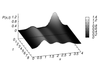
Figure 2: The supplementary 3d view showing the variation of $P(x,t)$ until the limiting distribution is attained. Calculated for the same conditions as in Fig. 1. The formation of ”tree-hill” (long-term) asymptotics is visible.

Figure 3: The non-equilibrium behavior of the Shannon entropy $S_{\rm sh}$ (part a) and Markovian entropy rate $S_{\rm mr}$ (part b). The complementary dependencies to those presented in Fig. 2) calculated for perturbations - 3 distinct environments with the same mean $\mu^{\rm e}=1$, but different dispersion $\sigma^{\rm e}=0.2,0.6,1.5$. The calculation shows the non-monotonously growing entropy (on the level of the clone) (see Eqs. (19,20)). The alternative information-theoretic measure, the Markovian entropy rate shows that transitions between attractors exhibit diversity decrease and saturation.

V Therapy as inverse problem

Despite the exclusively theoretical nature of our work, we outline its eventual contribution for therapy design. When the therapeutic intervention is to consist in purposeful manipulation with the statistics of the tumor microenvironment (represented here by the parameters $\mu^{\rm e},\sigma^{\rm e}$) aimed to reduce heterogeneity ($\propto S_{\rm sh})$, the therapy may be formally viewed as the entropy minimization problem and solved by standard optimization techniques Floudas2009 . To be more specific, the system of equations for $\sigma^{\rm e}(t)$ and $\mu^{\rm e}(t)$ can be written, that, in principle, represents steepest descent gradient dynamics towards their values in ’physiological’ or ’desired’ conditions, denoted by $\sigma^{\rm e}_{\rm des}$, $\mu^{\rm e}_{\rm des}$ and $s^{\rm e}_{\rm des}$

$$\frac{{\rm d}\ln\sigma^{\rm e}}{{\rm d}t} = -\frac{\partial d_{\rm ther}^{2}\,\,\,}{\partial\ln\sigma^{\rm e}}\,,$$ (21)

$$\frac{{\rm d}\mu^{\rm e}}{{\rm d}t} = -\frac{\partial d_{\rm ther}^{2}\,\,\,}{\partial\mu^{\rm e}}\,,$$

which minimizes objective function in the form of ’therapeutic’ weighted squared Euclidean distance

$$d_{\rm ther}^{2} = v_{S}\delta_{S}^{2}+v_{\sigma}\delta_{\sigma}^{2}+v_{\mu}\delta_{\mu}^{2}$$ (22)

consisting of the differences of desired and actual values of generalized coordinates

$$\delta_{S} = \ln S_{\rm sh,des}-\ln S_{\rm sh}\,,$$ (23)

$$\delta_{\sigma} = \ln\sigma_{\rm des}^{\rm e}-\ln\sigma^{\rm e}\,,$$

$$\delta_{\mu} = \mu_{\rm des}^{\rm e}-\mu^{\rm e}\,,$$

weighted by the respective constants $v_{S}>0$, $v_{\sigma}>0$, $v_{\mu}>0$. The term $\ln\sigma^{\rm e}$ is used instead of $\sigma^{\rm e}$ to keep the constraint $\sigma^{\rm e}\geq 0$ for any eventual solution. Under some conditions, proper choice of desired entropy value of $S_{\rm sh,des}\gtrsim 0$ can, in principle, provide formally correct entropy decrease, prevented, however, by the effect of $\delta_{\sigma}$, $\delta_{\mu}$, or by principal impossibility to decrease entropy beyond certain limits. The constant parameters $v_{\mu}$, $v_{\sigma}$ are used to bias optimization pressure from the values of $\mu^{\rm e}$, $\sigma^{\rm e}$ providing formally correct but, eventually, non-physiological solution ($\delta_{S}\sim 0$), towards their values $\mu_{\rm des}^{\rm e}$, $\sigma_{\rm des}^{\rm e}$ in standard physiological conditions.

We emphasize that the above therapeutic considerations are implied by applying the generalized distance-based concept as the crucial aspect of our approach. In this context it is worth mentioning that therapeutic model based on the construction of $d_{\rm ther}^{2}$ minimization pathway is inspired by the broad class of inverse problems discussed in Tarantola2004 . The above system of nonlinear equations (21) must be solved simultaneously with equations for $\{p_{i}(t)\}_{i=1}^{N}$ regarding instant $S_{\rm sh}$.

VI Conclusion

Here outlined Markovian-based conceptualization links the uncertainty of environment with intratumor heterogeneity, both expressed in probabilistic terms. Evolutionary nature of carcinogenesis Nowell1976 is respected, as the transition probabilities correlate with statistical match between environment and the attractors of the respective states, which corresponds to the bet-hedging strategy Dejong2011 , evolved in biological populations that face time-varying environment Muller2013 .

Recently, the evolutionary strategy called ’evolutionary trap’ was proposed Chen2015 . It consists of two steps, in which the first stress ’channels’ karyotypically divergent population into one with a predominant drugable karyotypic feature, the second stress targeting this feature Chen2015 . Here presented approach follows the same aim, to lower diversity of cancer cells population, in a more formal way. Therapy is formulated as the optimization problem, representing inverse modeling approach, which means evolving desired phenotypic heterogeneity by purposeful manipulating with the environment’s statistics. Here, the ’desired’ intratumor heterogeneity corresponds to probability distribution represented by the only peak, as narrow as possible. We believe that the combination of the more formal approach, as proposed here, with numerical simulations may provide interesting strategies, going beyond usual intuition.

This work was supported by the (i) Scientific Grant Agency of the Ministry of Education of Slovak Republic under the grant VEGA No. 1/0348/15, and (ii) CELIM (316310) funded by 7FP EU (REGPOT).

Appendix: Regularization of Hellinger distance for the pair of gaussian distributions

The purpose of this appendix is to review some elements of Hellinger distance calculus. We define the square of the Hellinger distance $d^{2}$ in terms of elementary probability theory. If we denote the parametrization of the probability densities as $\phi(x,\theta_{s})$, $s=1,2$, then the squared Hellinger distance can be expressed as

$$d^{2}(\theta_{1},\theta_{2})=1-\int_{-\infty}^{\infty}\sqrt{\phi(x,\theta_{1})\phi(x,\theta_{2})}{\rm d}x\,.$$ (24)

In the case of the pair of two Gaussian distributions $\phi_{g}(x,\mu_{1},\sigma_{1})$, $\phi_{g}(x,\mu_{2},\sigma_{2})$ constructed from the ”template”

$$\phi(x,\theta)\equiv\phi_{g}(x,\mu,\sigma)=\frac{1}{\sqrt{2\pi}\sigma}\exp\left[-\frac{(x-\mu)^{2}}{2\sigma^{2}}\right]$$ (25)

we obtained

$$\begin{split}d^{2}(\mu_{1},\sigma_{1},\mu_{2},\sigma_{2})=\ \ \ \ \ \ \ \ \ \ \ \ \ \ \ \ \ \ \ \ \ \ \ \ \ \ \ \ \ \ \ \ \ \ \ \ \ \ \ \ \ \ \ \ \\ 1-\sqrt{\frac{2\sigma_{1}\sigma_{2}}{\sigma_{1}^{2}+\sigma_{2}^{2}}}\exp\left(-\frac{(\mu_{1}-\mu_{2})^{2}}{4(\sigma_{1}^{2}+\sigma_{2}^{2})}\right)\,.\end{split}$$ (26)

Since the limit $(\sigma_{1},\sigma_{2})\rightarrow(0,0)$ may create the interpretation problems, the original form of $d^{2}(.)$ should be regularized. One possible way is to use additive extra dispersion $\epsilon>0$ as follows

$$\begin{split}d^{2}(\mu_{1},\sigma_{1},\mu_{2},\sigma_{2},\epsilon)=1-\sqrt{\frac{2(\sigma_{1}+\epsilon)(\sigma_{2}+\epsilon)}{(\sigma_{1}+\epsilon)^{2}+(\sigma_{2}+\epsilon)^{2}}}\\ \times\exp\left(-\frac{(\mu_{1}-\mu_{2})^{2}}{4((\sigma_{1}+\epsilon)^{2}+(\sigma_{2}+\epsilon)^{2})}\right)\,.\end{split}$$ (27)

Thus, in the case when the original dispersions $\sigma_{1},\sigma_{2}$ shrink to zero we have

$$d^{2}(\mu_{1},0,\mu_{2},0,\epsilon)=1-\exp\left(-\frac{(\mu_{1}-\mu_{2})^{2}}{8\epsilon^{2}}\right)\,.$$ (28)

Then the Taylor expansion of the previously obtained function at $\mu_{1}\sim\mu_{2}$ yields

$$\begin{split}d^{2}(\mu_{1},0,\mu_{2},0,\epsilon)=\ \ \ \ \ \ \ \ \ \ \ \ \ \ \ \ \ \ \ \ \ \ \ \ \ \ \ \ \ \ \ \ \ \ \ \ \ \ \ \ \ \ \ \ \\ \frac{(\mu_{1}-\mu_{2})^{2}}{8\epsilon^{2}}-\frac{(\mu_{1}-\mu_{2})^{4}}{128\epsilon^{4}}+{\cal O}((\mu_{1}-\mu_{2})^{6})\,\end{split}$$ (29)

with the leading term proportional to the dissimilarity measure analogous to the one dimensional quadratic Euclidean squared distance $(\mu_{1}-\mu_{2})^{2}$ between Cartesian coordinates $\mu_{1}$ and $\mu_{2}$ in 1d. Such demonstration of the asymptotic consistency between generalized distance measure of the probability distributions and classical analytical Euclidean distance in 1d supports the adequacy of $\epsilon>0$ regularization.

The derivation highlights the interesting connection between traditional geometric and functional distance measures. A further perspective in the analysis of tumors consisting of several spatial compartments should also be mentioned. In such case, the consequences of random switching could be readily quantified using Lukaszyk-Karmowski distance $\int{\rm d}\mu_{1}\int{\rm d}\mu_{2}\,\pi(\mu_{1})\pi(\mu_{2})|\mu_{1}-\mu_{2}|$ Lukaszyk2003 , which specifies geometric distance of the points with coordinates $\mu_{1}$ and $\mu_{2}$ known up to the respective probability distributions $\pi(\mu_{1})$, $\pi(\mu_{2})$.

References

- (1) A. Marusyk, K. Polyak, Science 339, 528 (2013)
- (2) M. M. Gottesman, Annu. Rev. Med. 53, 615 (2002)
- (3) S. J. Altschuler, L. F. Wu, Cell 141, 559 (2010)
- (4) N. D. Marjanovic, R. A. Weinberg, C. L. Chaffer, Clin. Chem. 59, 253 (2013)
- (5) S. Huang, Cancer Metastasis Rev. 32, 423 (2013)
- (6) K. Kemper, P. L. de Goeje, D. S. Peeper, R. van Amerongen, Cancer Res. 74, 5937 (2014)
- (7) W. L. Tam, R. A. Weinberg, Nat. Med. 19, 1438 (2013)
- (8) W. M. ElShamy, R. J. Douhé, Cancer Lett. 341, 2 (2013)
- (9) N. A. Saunders, et al., EMBO Mol. Med. 4, 675 (2012)
- (10) S. T. Buckland, A. E. Magurran, R. E. Green, R. M. Fewster, Phil. Trans. R. Soc. B 360, 243 (2005)
- (11) C. J. Keylock, OIKOS 109, 203 (2005)
- (12) R. S. Mendes, L. R. Evangelista, S. M. Thomaz, A. A. Agostinho, L. C. Gomes, Ecography 31, 450 (2008)
- (13) L. Preziosi, Cancer Modeling and Simulation, CRC Press (2003)
- (14) C. Maenhaut, J. E. Dumont, P. P. Roger, W. C. G. Staveren, Carcinogenesis 31, 149 (2010)
- (15) H. H. Chang, M. Hemberg, M. Barahona, D. E. Ingber, S. Huang, Nature 453, 544 (2008)
- (16) E. Quintana, et al., Cancer Cell 18, 510 (2010)
- (17) S. V. Sharma, et al., Cell 141, 69 (2010)
- (18) K. S. Hoek, C. R. Goding, Pigment Cell Melanoma Res. 23, 746 (2010)
- (19) C. L. Chaffer, et al., Proc. Natl. Acad. Sci. USA 108, 7950 (2011)
- (20) P. B. Gupta, et al., Cell 146, 633 (2011)
- (21) K. Binder, D. W. Heermann, Monte Carlo Simulation in Statistical Physics: An Introduction, Springer-Verlag (2002)
- (22) P. J. Choi, L. Cai, K. Frieda, S. Xie, Science 322, 442 (2008)
- (23) A. Raj, A. van Oudenaarden, Cell 135, 216 (2008)
- (24) A. Eldar, M. B. Elowitz, Nature 467, 167 (2010)
- (25) U. Liberman, J. V. Cleve, M. W. Feldman, Genetics 187, 837 (2011)
- (26) E. Pujadas, A. P. Feinberg, Cell 148, 1123 (2012)
- (27) E. Kussell, S. Leibler, Science 309, 2075 (2005)
- (28) E. Kussell, R. Kishony, N. Q. Balaban, S. Leibler, Genetics 169, 1807 (2005)
- (29) M. Acar, J. T. Mettetal, A. van Oudenaarden, Nat. Genet. 40, 471 (2008)
- (30) W. E. Frankenhuis, K. Panchanathan, Proc. R. Soc. Lond. B 278, 3558 (2011)
- (31) E. Libby, P. B. Rainey, Proc. R. Soc. Lond. B 278, 3574 (2011)
- (32) D. Fudenberg, L. A. Imhof, Bull. Math. Biol. 74, 399 (2012)
- (33) S. Fedotov, A. Iomin, Phys. Rev. Lett. 98, 118101 (2007)
- (34) S. Fedotov, A. Iomin, Phys. Rev. E 77, 031911 (2008)
- (35) P. C. Nowell, Science 194, 23 (1976)
- (36) L. M. F. Merlo, J. W. Pepper, B. J. Reid, C. C. Maley, Nat. Rev. Cancer 6, 924 (2006)
- (37) M. Greaves, Nat. Rev. Cancer 7, 213 (2007)
- (38) L. López-Maury, S. Marguerat, J. Bähler, Nat. Rev. Genet. 9, 583 (2008)
- (39) J. X. Zhou, M. D. S. Aliyu, E. Aurell, S. Huang, J. R. Soc. Interface 9, 3539 (2012)
- (40) M. B. Elowitz, A. J. Levine, E. D. Siggia, P. S. Swain, Science 297, 1183 (2002)
- (41) H. Crauel, A. Debussche, F. Flandoli, J. Dynam. Differential Equations 9, 307 (1997)
- (42) J. Braun, M. Mattia, NeuroImage 52, 740 (2010)
- (43) O. Stiller, A. Becker, L. Kramer, Phys. Rev. Lett. 68, 3670 (1992)
- (44) M. C. Donaldson-Matasci, M. Lachmann, C. T. Bergstrom, Evol. Ecol. Res. 10, 493 (2008)
- (45) E. Hellinger, J. Reine Angew. Math. 1909, 210 (1909)
- (46) C. Hesse, D. Holtackers, T. Heskes, in Proceedings of the 1st Annual Symposium IEEE EMBS Benelux Chapter, Brussels, Belgium (2006)
- (47) D. Hull, The Metaphysics of Evolution, Stony Brook: State University of New York Press (1989)
- (48) A. Solopova, et al., Proc. Natl. Acad. Sci. USA 111, 7427 (2014)
- (49) H. Kuwahara, O. S. Soyer, Mol. Syst. Biol. 8, art. 564 (2012)
- (50) C. A. Floudas, P. M. P. (eds.), Encyclopedia of Optimization, Springer (2009)
- (51) A. Tarantola, Inverse Problem Theory and Methods for Model Parameter Estimation, Society for Industrial and Applied Mathematics, Philadelphia, PA, USA (2004)
- (52) I. de Jong, P. Haccou, O. P. Kuipers, BioEssays 33, 215 (2011)
- (53) J. Müller, B. A. Hense, T. M. Fuchs, M. Utz, C. Pötzsche, J. Theor. Biol. 336, 144 (2013)
- (54) G. Chen, et al., Cell 160, 771 (2015)
- (55) S. Lukaszyk, Comput. Mech. 33, 299 (2003)