Upper limits to the magnetic field in central stars of planetary nebulae
Abstract
More than about twenty central stars of planetary nebulae (CSPN) have been observed spectropolarimetrically, yet no clear, unambiguous signal of the presence of a magnetic field in these objects has been found. We perform a statistical (Bayesian) analysis of all the available spectropolarimetric observations of CSPN to constrain the magnetic fields on these objects. Assuming that the stellar field is dipolar and that the dipole axis of the objects are oriented randomly (isotropically), we find that the dipole magnetic field strength is smaller than 400 G with 95% probability using all available observations. The analysis introduced allows integration of future observations to further constrain the parameters of the distribution, and it is general, so that it can be easily applied to other classes of magnetic objects. We propose several ways to improve the upper limits found here.
Subject headings:
magnetic fields — polarization — techniques: polarimetric — methods: data analysis, statistical1. Introduction
The detection of magnetic fields in the CSPN has been a subject of considerable interest recently. The presence of magnetic fields on CSPN could shed some light on the magnetic field of planetary nebulae (PNe) themselves, and hence on the role of magnetic fields on the shaping of PNe (Chevalier & Luo, 1994; Tweedy et al., 1995; García-Segura et al., 1999; Blackman et al., 2001a, b; Balick & Frank, 2002; Soker, 2004, 2006; Vlemmings et al., 2006; Sabin et al., 2007). Yet, magnetic fields on CSPN have proved elusive and so far, no clear, unambiguous spectropolarimetric detection of a magnetic field in a CSPN has been possible (Leone et al., 2011; Bagnulo et al., 2012; Jordan et al., 2012).
Spectropolarimetry of CSPN is challenging because they are intrinsically faint and must be observed at relatively low spectral resolutions, which leads to cancellations attenuating the, already weak, polarimetric signals. Additionally, CSPN present a relatively low number of spectral lines, which hampers line addition techniques that exploit the collective contribution of hundreds (or even thousands) of spectral lines to increase the signal-to-noise ratio (Semel & Li, 1996; Donati et al., 1997; Martínez González et al., 2008).
Here we follow a different approach. We aim at constraining the magnetic field on CSPN statistically, combining the overall information of all available observations to constrain the magnetism of CSPN (in a way similar, but more general, to the analysis of magnetic fields in RR Lyrae of Kolenberg & Bagnulo, 2009). A common procedure would be combining the inferred values of the field strengths (obtained for example, from least-squares fitting) in a histogram. However, this is unsuitable because on the one hand, noise introduces large uncertainties and degeneracies in the determination of the field that are not properly propagated when carrying out a histogram; and on the other, the magnetic field is not a directly measurable quantity, it is inferred from observations. Consequently, a robust inference of the distribution of magnetic fields in CSPN is better done within the Bayesian formalism (see Bovy et al., 2011, 2011 for a similar approach). In fact, we will follow a hierarchical Bayesian approach similar to that recently follower by Hogg et al. (2010) to estimate the distribution of eccentricities in the orbits of binary stars and exoplanets; but unlike them, here, we carry out the full hierarchical Bayesian analysis.
2. Magnetic field inference under a Bayesian hierarchical analysis
In magnetized atmospheres, spectral lines show a characteristic circular polarization pattern dominated by the Zeeman effect. If the Zeeman splitting is sufficiently small so that it does not dominate the broadening of the spectral lines, and assuming that the magnetic field is roughly constant along the line of sight (LOS) and has a dipolar topology in the stellar surface, this circular polarization flux pattern can be simply modeled as (see Landi Degl’Innocenti, 1992; Martínez González et al., 2012)
| (1) |
where is the intensity flux, and , with being the magnetic field strength in the pole and the inclination of the dipole axis with respect to the LOS. Additionally, in the absence of limb darkening (see Martínez González et al., 2012, for the general expression), is the central wavelength of the spectral line (in Å), and is the effective Landé factor of the transition (Landi Degl’Innocenti, 1982). For a general discussion about the weak-field approximation in stellar magnetism, we refer to Martínez González et al. (2012). From the observational point of view, is easier to measure because it is less prone to errors (e.g., Bagnulo et al., 2009). Consequently, we work instead with
| (2) |
Although all the subsequent formalism is presented in terms of to simplify the notation, they are still valid provided one substitutes for and for .
A number of different methods have been devised to infer the magnetic field of an object from a set of observations of the flux of the Stokes and Stokes spectra at some given wavelengths . Maximum likelihood methods consist on choosing the parameter(s) that maximizes the likelihood function , which is the probability of observing the data (here, the intensity and polarization profiles), given the physical parameters of the model (here, the average longitudinal magnetic field) (e.g., Jaynes & Bretthorst, 2003; Martínez González et al., 2012). The likelihood ensues simply from equation (1) and our model for the noise (here, Gaussian; see Appendix):
| (3) |
where extends over all the spectral lines in the observed spectrum (each with wavelengths), and are the variances of the Gaussian noise of the circular polarization profile and the derivative of the intensity respectively, and and are combination of averages of the observed and defined in the Appendix. The denominator of each term in the exponential can be understood as (twice) the variance of the linear combination of the two random variables and : , assuming that is the average correlation between and (Press et al., 1992; Asensio Ramos & Manso Sainz, 2011). For typical modulation schemes, . Hence, , where is the spectral resolution and the characteristic wavelength. In the optical ( Å), for , and for relatively weak fields, the second and third terms can be neglected so that equation (3) simplifies to
| (4) |
where and have been redefined as in equation (A8) (for clarity, the explicit dependence of on the spectral line is not shown). Note that is the maximum likelihood estimate for (see Martínez González et al., 2012; Leone et al., 2013).
In a Bayesian analysis, the a posteriori probability for the presence of a magnetic field in the object given some observations is simply obtained from the Bayes theorem (e.g., Jaynes & Bretthorst, 2003; Gregory, 2005)
| (5) |
where , measures our a priori knowledge on the value of the field, and is the so-called evidence, which we will not consider explicitly in the following since it is just a scaling factor so that the posterior is normalized (). There is, in principle, no a priori reason for the field pointing towards us or away from us, and it seems likely that the most probable value of be zero. Hence, a natural choice for would be a normal distribution for some fixed variance (which can be potentially very large). Equation (5) may thus be used to infer the magnetic field of an object from polarimetric observations (see, for example, Asensio Ramos et al., 2007; Asensio Ramos, 2009, 2011). Instead, here, we are interested on the statistical distribution of all of them and how this distribution is constrained by the observations.
| Object (PNe) | [G]aafootnotemark: | [G] (with error)bbfootnotemark: | ||
|---|---|---|---|---|
| NGC 2392 | 4 | 1.310-7 | ||
| NGC 1360 | 12 | 3.210-8 | ||
| NGC 1360 | 16 | 2.910-8 | ||
| NGC 1360 | 4 | 8.210-7 | ||
| NGC 6826 | 12 | 2.110-7 | ||
| NGC 6826 | 4 | 3.210-9 | ||
| PHL 932 | 20 | 2.310-8 | ||
| LSS 1362 | 4 | 1.610-7 | ||
| Abell 36 | 8 | 3.810-7 | ||
| Abell 36 | 12 | 4.410-7 | ||
| IC 4637 | 4 | 2.810-7 | ||
| LSE 125 | 12 | 1.410-6 | ||
| LSE 125 | 4 | 2.010-7 | ||
| NGC 4361 | 7 | 2.010-7 | ||
| NGC 7293 | 2 | 4.110-9 | ||
| Tc 1 | 6 | 2.910-7 | ||
| Tc 1 | 1 | 1.910-8 | ||
| NGC 6026 | 30 | 1.810-6 | ||
| HD 44179 | 16 | 2.310-5 |
We now make the simplification of assuming that all observations are statistically independent. In other words, observing an object tells you nothing about the magnetic field of another one. Repeated observations of the same star are modeled by using the same unless the observations are obtained in too different epochs. In this case, they are considered to be different objects because of the potential variability of the source. Strictly speaking, the assumption of independence is surely not correct for different observations of the same star at different epochs and one should include the covariance between them. However, we make this simplification for the sake of obtaining a simpler analytical final result and because this covariance is difficult to model and estimate. If the previous conditions hold, we can factorize the likelihood and the priors so that the posterior reads
| (6) |
where is the set of all the observed Stokes profiles averaged over the stellar surface, , and is a Gaussian with mean 0 and variance . Instead of using a fixed , we follow a hierarchical Bayesian approach and we introduce into the Bayesian inference scheme (Gregory, 2005), so that
| (7) |
The parameters is then termed hyperparameter, since it is a parameter of the prior. Note that is does not affect the likelihood. The joint prior for and can be factorized as
| (8) |
so that the marginal prior for could be obtained by marginalizing (i.e., integrating out)
| (9) |
As discussed above, we consider . Integrating equation (6) over all the variables (using equation [4]), the marginalized posterior for is obtained, resulting in
| (10) |
where is given by
| (11) |
while is the prior to be chosen over the hyperparameter . The previous expression can be considered as a multiobject and multiline approach to magnetic field detection.
We do not have any a priori information on , which is a scale variable. A convenient uninformative prior in these cases is the Jeffreys prior because it distributes probability uniformly in the logarithm: it is as likely to find between 0.1 and 1 G, as between 10 and 100 G (Jeffreys, 1968; Jaynes & Bretthorst, 2003). This prior is improper (its integral is not finite) and here, it yields an improper posterior too. For that reason, a cutoff has to be chosen. For any informative data set (peaked ), the value of the cutoff becomes irrelevant but for, perhaps, ridiculously small values; for less informative (i.e., flatter) , we must check the sensitivity of the results to the value of .
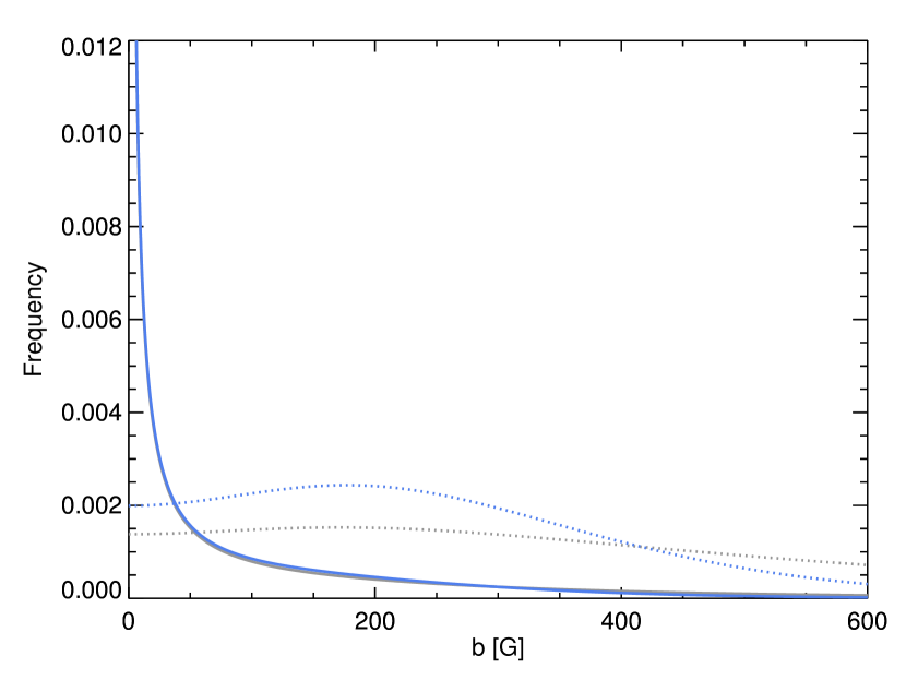
Figure 1 shows, in grey, (dotted line) and the posterior using a Jeffreys’ prior (solid line) for the CSPN data compiled in Leone et al. (2013) and summarized in table 1. A characteristic of the likelihood displayed in equation (11) is that it only depends on the maximum likelihood estimation of the longitudinal field, and of the coefficients (the coefficients represent just a scaling of the likelihood and are of no importance for our purpose). According to equation (A9), can be obtained from the uncertainty in the estimation of , as computed by Martínez González et al. (2012). Therefore, we can make use of the recent results of Jordan et al. (2012) and use their estimations to upgrade our observations. Note that, since their results represent a longitudinal magnetic field averaged on the stellar surface, they have to be multiplied by 4 to account for the dipolar dilution (Martínez González et al., 2012). According to Fig. 1, the addition of the observations of Jordan et al. (2012) barely modifies the posterior distribution . The results point to a very small value of .
From the posterior of the hyperparameter, we derive the posterior probability of the longitudinal field for all the sources as
| (12) |
This distribution depends on the cut-off , but only weakly for ranging between - G. Although we do not display the figure, choosing mG, is below 250 G in absolute value with 95% probability.
More interesting is to consider the distribution of , the magnetic field strength of the dipole, which can be obtained from the distribution of assuming that the dipole inclination angle of the different CSPN is randomly (isotropically) oriented in space, which seems reasonable since there is no clear evidence for a preferential orientation of PNe themselves (Corradi et al., 1998). This computation is not possible in the general case in which is interpreted as an average longitudinal field over the stellar surface. Then, a-priori, follows a Maxwellian distribution:
| (13) |
Proceeding as above we derive the distribution of dipolar magnetic field strength from all the observed sources as
| (14) |
It is interesting to compare this equation with Eq. (7) of Kolenberg & Bagnulo (2009) and point out the differences. Although the two formalism assume an isotropic distribution of fields, our approach is more general for the following reasons: i) we use a fully Bayesian approach in which we model the observed Stokes profiles to correctly propagate all uncertainties in the observations to the magnetic field distribution, while Kolenberg & Bagnulo (2009) use the maximum likelihood estimation of the and ii) we take into account that each source can have a different magnetic field strength and that it is known with imprecision.
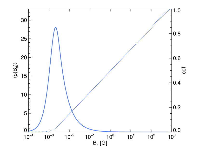
Figure 2 shows the corresponding probability density function (solid) and the cumulative distribution (dotted) for the data of Leone et al. (2013) alone and what happens when we add the data of Jordan et al. (2012). From this, the dipolar magnetic field strength is larger than 3 mG and smaller than 400 G with 95% probability. Note that this result is independent of , since equation (14) is not divergent for , unlike equation (12).
3. Discussion and conclusions
An important property of is its ability to concentrate for large . Consider, for example, an ensemble of objects with similar spectra that are observed with identical uncertainties (hence, they have similar ); they only differ in their magnetic field strength (i.e., ). Then, the maximum of (or ) in equation (11) will lie at
| (15) |
where . In the first case, the observations are inadequate (too noisy, and therefore, too large), for the estimated to be informative. is relatively flat near and when multiplied by the Jeffreys prior, the posterior clearly diverges towards smaller values, always reaching its maximum a-posteriori (MAP) value at the cut-off, , which is not very helpful. An illustration of this situation is given by one of the dotted lines in figure 3, which corresponds to an incomplete subset of just four observed objects from table 1. The two other dotted lines correspond to different subsets with the same number of objects. In those other cases, has a maximum at some non-zero value , which is noticeable also in the posterior . But they are notably wider (spanning several hundreds of gauss) than the likelihood obtained from the full set of observed objects (gray solid line). In fact, it can be shown that for large values of , the width of converges to 0 as . Therefore, becomes more and more informative on the value of as we accumulate observations (), even if the individual observations are too noisy to get a clear detection (cf. solid gray line in Figure 3). In a sense, this is a generalization of multiline addition techniques in which the collective contribution of many individual spectral lines from an object is used to increase the signal-to-noise ratio of the polarization pattern (Semel & Li, 1996; Donati et al., 1997; Martínez González et al., 2008). Here, the collective contribution of many different objects contribute to constrain the statistical distribution of fields.
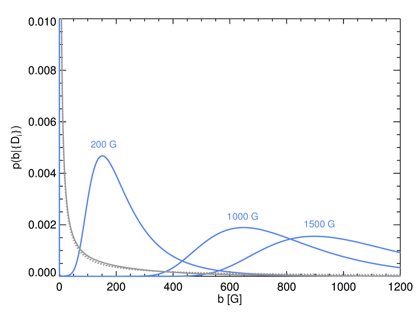
It is also interesting to see how a few better observations may affect the estimates. For example, consider that we observed two objects with well-defined , but with a much better precision than up to now (say, is a factor 100 better), i.e., in case we had a clear detection for some (perhaps, different) object. Figure 3 shows how change from the original (solid grey line) for three different values of . Likewise, we also display in dotted grey line what happens if we only take into account 4 of the available observations. This demonstrates that, although there is not a single detection of magnetic fields, adding more objects produces a collapse of the posterior.
We have introduced two major simplifications in the method which are not essential. The first one regards noise estimation. We have assumed that the variance of the observed quantities ( and ) was known for the derivation the likelihood functions (see Appendix), and that they are independent of wavelength. Their actual values have been independently estimated from the intensity fluctuations in the continuum windows between spectral lines. Estimating the unknown variance of a set of measurements is a fundamental problem in Bayesian theory which can be done independently (like here) or consistently within the Bayesian analysis itself by assigning (e.g., non-informative, Jeffreys) priors to and , and marginalizing these parameters. We have not pursued this more general approach here to keep our main argument simple.
Secondly, the approximation in equation (4) has allowed the analytical derivation of equation (11). This approximation is accurate beyond the strict limits stated above. When the more general equation (3) is required, the integrals in equation (11) have to be performed numerically using Markov Chain Monte Carlo methods or alike, depending on the dimensionality of the problem.
An important characteristic of the analysis presented is that it naturally allows integration of new data to improve the magnetic field estimates. We have already shown how things change when the data of Jordan et al. (2012) is added to the observations of Leone et al. (2013). From the analysis of all the available observations so far we have obtained the upper-limit of 400 G.
Our analysis here suggests several ways in which such estimates can be improved. As shown above, the mere addition of new observations helps constraining the magnetic field distribution, even when no clear detection in the individual objects is possible. The constraints on the global distribution can be even stronger when either the new observations have a better (lower) noise level, or if clear detection on individual objects is achieved.
The analysis presented in this paper is not limited to any particular spectral range, provided that the weak-field approximation holds. Observations at different spectral windows can be straightforwardly included in the analysis after computing their corresponding , , and values (although in some cases it might be advisable to consider the general expression for the likelihood (Eq. (3)). Given that the amplitude of the Zeeman Stokes scales with (see, e.g., Landi Degl’Innocenti & Landolfi, 2004), spectropolarimetry of the Paschen and Brackett series should be favoured.
The joint analysis of linear and circular polarization would impose stronger constrains on the magnetic field distribution under the, very likely, assumption of isotropic distribution of fields for the observed objects. The Zeeman effect generates linear polarization patterns which are usually smaller than those of circular polarization and that are, in the weak-field approximation, proportional to the square of the transversal component of the magnetic field to the LOS (e.g., Landi Degl’Innocenti, 1992; Landolfi et al., 1993; Martínez González et al., 2012). However, we understand that the detection of linear polarization is extremely improbable, given that no reliable detection of circular polarization has been achieved so far.
Additionally, magnetic alignment of dust grains creates linear polarization in the continuum from which we may infer the presence of a magnetic field (e.g., Davis & Greenstein, 1951; Lazarian, 2007). The information thus obtained is not quantitative and cannot be directly included in our formalism. Yet, it may provide important general and symmetry constraints and bounds that could be implemented within the Bayesian methodology.
Finally, it is clear that the approach presented here can be applied to other sets of objects (e.g., white dwarfs, …) once they can be assumed to belong to the same magnetic class, i.e., they are all characterized by the same statistical distribution of fields.
Appendix A Computation of the likelihood
We assume that the observed circular polarization flux is given by equation (1) but that it is corrupted by a normaly distributed noise with zero mean and variance :
| (A1) |
the flux derivative, in turn, is corrupted by a noise :
| (A2) |
Assuming that both sources of error are independent, then the joint likelihood of the data is
| (A3) |
The true value is treated as a nuisance parameter that we may integrate out for some uniform vague prior
| (A4) |
Assuming statistical independence for the wavelengths, and constant and accross the spectral line,
| (A5) |
where, introducing the notation , , , then,
Note that , and implicitly depend on the spectral line considered and also explicitly through the effective Landé factor within . Extending the argument to all the spectral lines
| (A6) |
where represents the wavelength point of line . In equation (A6), and are, in principle, different for the each spectral line; they are estimated from their adjacent continuum (for clarity, we do not write the subscript ). To second order on ,
| (A7) |
where
| (A8) |
with ; ; and . Interestingly, the coefficient can be related to the error bar of as shown by Martínez González et al. (2012)
| (A9) |
Therefore, all the ingredients to carry out our calculations are readly available from any work that tabulates the maximum-likelihood estimation of the longitudinal field and its associated error bar.
References
- Asensio Ramos (2009) Asensio Ramos, A. 2009, ApJ, 701, 1032
- Asensio Ramos (2011) —. 2011, ApJ, 731, 27
- Asensio Ramos & Manso Sainz (2011) Asensio Ramos, A., & Manso Sainz, R. 2011, ApJ, 731, 125
- Asensio Ramos et al. (2007) Asensio Ramos, A., Martínez González, M. J., & Rubiño-Martín, J. A. 2007, A&A, 476, 959
- Bagnulo et al. (2009) Bagnulo, S., Landolfi, M., Landstreet, J. D., Landi Degl’Innocenti, E., Fossati, L., & Sterzik, M. 2009, PASP, 121, 993
- Bagnulo et al. (2012) Bagnulo, S., Landstreet, J. D., Fossati, L., & Kochukhov, O. 2012, A&A, 538, A129
- Balick & Frank (2002) Balick, B., & Frank, A. 2002, ARA&A, 40, 439
- Blackman et al. (2001a) Blackman, E. G., Frank, A., Markiel, J. A., Thomas, J. H., & Van Horn, H. M. 2001a, Nature, 409, 485
- Blackman et al. (2001b) Blackman, E. G., Frank, A., & Welch, C. 2001b, ApJ, 546, 288
- Bovy et al. (2011) Bovy, J., Hennawi, J. F., Hogg, D. W., Myers, A. D., Kirkpatrick, J. A., Schlegel, D. J., Ross, N. P., Sheldon, E. S., McGreer, I. D., Schneider, D. P., & Weaver, B. A. 2011, ApJ, 729, 141
- Chevalier & Luo (1994) Chevalier, R. A., & Luo, D. 1994, ApJ, 421, 225
- Corradi et al. (1998) Corradi, R. L. M., Aznar, R., & Mampaso, A. 1998, MNRAS, 297, 617
- Davis & Greenstein (1951) Davis, Jr., L., & Greenstein, J. L. 1951, ApJ, 114, 206
- Donati et al. (1997) Donati, J.-F., Semel, M., Carter, B. D., Rees, D. E., & Collier Cameron, A. 1997, MNRAS, 291, 658
- García-Segura et al. (1999) García-Segura, G., Langer, N., Różyczka, M., & Franco, J. 1999, ApJ, 517, 767
- Gregory (2005) Gregory, P. C. 2005, Bayesian Logical Data Analysis for the Physical Sciences: A Comparative Approach with ‘Mathematica’ Support (Cambridge: University Press)
- Hogg et al. (2010) Hogg, D. W., Myers, A. D., & Bovy, J. 2010, ApJ, 725, 2166
- Jaynes & Bretthorst (2003) Jaynes, E. T., & Bretthorst, G. L. 2003, Probability Theory, the Logic of Science (Cambridge: University Press)
- Jeffreys (1968) Jeffreys, H. 1968, Theory of Probability (Oxford: University Press)
- Jordan et al. (2012) Jordan, S., Bagnulo, S., Werner, K., & O’Toole, S. J. 2012, A&A, 542, A64
- Kolenberg & Bagnulo (2009) Kolenberg, K., & Bagnulo, S. 2009, A&A, 498, 543
- Landi Degl’Innocenti (1982) Landi Degl’Innocenti, E. 1982, Sol. Phys., 77, 285
- Landi Degl’Innocenti (1992) —. 1992, Magnetic field measurements, ed. F. Sánchez, M. Collados, & M. Vázquez (Cambridge: University Press), 71
- Landolfi et al. (1993) Landolfi, M., Landi Degl’Innocenti, E., Landi Degl’Innocenti, M., & Leroy, J. L. 1993, A&A, 272, 285
- Landi Degl’Innocenti & Landolfi (2004) Landi Degl’Innocenti, E. & Landolfi, M. 2004, Polarization in Spectral Lines (Kluwer Academic Publishers)
- Lazarian (2007) Lazarian, A. 2007, JQSRT, 106, 225
- Leone et al. (2013) Leone, F., Martínez González, M. J., Corradi, R. L. M., Asensio Ramos, A., & Manso Sainz, R. 2014, A&A, 563, A43
- Leone et al. (2011) Leone, F., Martínez González, M. J., Corradi, R. L. M., Privitera, G., & Manso Sainz, R. 2011, ApJL, 731, L33
- Martínez González et al. (2008) Martínez González, M. J., Asensio Ramos, A., Carroll, T. A., Kopf, M., Ramírez Vélez, J. C., & Semel, M. 2008, A&A, 486, 637
- Martínez González et al. (2012) Martínez González, M. J., Manso Sainz, R., Asensio Ramos, A., & Belluzzi, L. 2012, MNRAS, 419, 153
- Press et al. (1992) Press, W. H., Teukolsky, S. A., Vetterling, W. T., & Flannery, B. P. 1992, Numerical recipes in FORTRAN. The art of scientific computing (Cambridge: University Press)
- Sabin et al. (2007) Sabin, L., Zijlstra, A. A., & Greaves, J. S. 2007, MNRAS, 376, 378
- Semel & Li (1996) Semel, M., & Li, J. 1996, Sol. Phys., 164, 417
- Soker (2004) Soker, N. 2004, in ASP Conf. Series, Vol. 313, Asymmetrical Planetary Nebulae III: Winds, Structure and the Thunderbird, ed. M. Meixner, J. H. Kastner, B. Balick, & N. Soker, 562
- Soker (2006) Soker, N. 2006, PASP, 118, 260
- Tweedy et al. (1995) Tweedy, R. W., Martos, M. A., & Noriega-Crespo, A. 1995, ApJ, 447, 257
- Vlemmings et al. (2006) Vlemmings, W. H. T., Diamond, P. J., & Imai, H. 2006, Nature, 440, 58