Models of parton distributions and the description of form factors of nucleon.

Abstract

The comparative analysis of different sets of the parton distribution functions (PDFs), based on the description of the whole sets of experimental data of electromagnetic form factors of the proton and neutron, is made in the framework of the model of t dependence of the generalized parton distributions (GPDs) with minimum free parameters and some extending variants of the model. In some cases, a large difference in the description of electromagnetic form factors of nucleons with using the different sets of PDF are found out. The different variants of the flavor dependence of the up and down quark form factors are presented and discussed. The gravitation form factors, obtained with the different sets of PDF, are also calculated and the anomalous gravimagnetic moment is compared with the equivalence principle. The calculations of the differential cross sections of the real Compton scattering are presented.

I Introduction

The structure of nucleons is the most intriguing problem of the old and new physics. In the first place, it is connected with the electromagnetic structure of the nucleon which can be obtained from the electron-hadron elastic scattering. In the Born approximation, the Feynman amplitude for the elastic electron-proton scattering Lomon is

$$M_{ep\rightarrow ep}=\frac{1}{q^{2}}[e\bar{u}(k_{2})\gamma^{\mu}u(k_{1}][e\bar{U}(p_{2}\Gamma_{\mu}(p_{1},p_{2})U(p_{1}],$$ (1)

where $u$ and $U$ are the electron and nucleon a Dirac spinors,

$$\Gamma^{\mu}=F_{1}(t)\gamma^{\mu}\ +\ F_{2}(t)\frac{i\sigma^{\mu\nu}q_{\nu}}{2m},$$ (2)

where $m$ is the nucleon mass, $\kappa$ is the anomalous part of the magnetic moment and $t=-q^{2}=-(p-p^{\prime})^{2}$ is the square of the momentum transfer of the nucleon.

The functions $F_{1}(t)$ and $F_{2}(t)$ are named the Dirac and Pauli form factors, which depend upon the nucleon structure. The normalization of the form factors QA12 is given by

$$F_{1}^{p}(t=0)=1,\ \ \ F_{2}^{p}(t=0)=\kappa_{p}=1.793$$ (3)

for the proton and

$$F_{1}^{n}(t=0)=0,\ \ \ F_{2}^{n}(t=0)=\kappa_{n}=-1.913$$ (4)

for the neutron.

Two important combinations of the Dirac and Pauli form factors are the so-called Sachs form factors Ernst60 ; Sachs62 . In the Breit frame the current is separated into the electric and magnetic contributions Kelly-02

$$\bar{u}(p^{\prime},s^{\prime})\Gamma^{\mu}u(p,s)=\chi^{{\dagger}}_{s^{\prime}}\left(G_{E}(t)+\frac{i\vec{\sigma}\times\vec{q_{B}}}{2m}G_{M}(t)\right)\chi_{s},$$ (5)

where $\chi_{s}$ is the two-component of the Pauli spinor, $G_{E}(t)$ and $G_{M}(t)$ are the Sachs form factors given by

$$G_{E}^{p/n}(t)=F_{1}^{p/n}(t)-\tau F_{2}^{p/n}(t),$$ (6)

$$G_{M}^{p/n}(t)=F_{1}^{p/n}(t)+F_{2}^{p/n}(t),$$ (7)

where $\tau=t/(4M^{2})$. Their three-dimensional Fourier transform provides the electric charge density and the magnetic current density distribution Sachs62 . Those form factors can be extracted from experimental data on the elastic electron-nucleon scattering by the Rosenbluth method or from the polarization electron proton elastic scattering.

Some experiments were based on the Rosenbluth formula Rosenbluth

$$\frac{d\sigma}{d\Omega}=\frac{\sigma_{Mott}}{\epsilon(1+\tau)}[\tau G^{2}_{M}(t)+\epsilon G^{2}_{E}(t)],$$ (8)

where $\tau=Q^{2}/4M^{2}_{p}$ and $\epsilon=[1+2(1+\tau)\tan^{2}(\theta_{e}/2)]^{-1}$ is the measure of the virtual photon polarization. Early experiments at modest $t$, based on the Rosenbluth separation method, suggested that the scaling behavior of both the proton form factors and the neutron magnetic form factor approximately described by a dipole form

$$G^{p}_{E}(t)\approx\frac{G^{p}_{M}(t)}{\mu_{p}}\approx\frac{G^{n}_{M}(t)}{\mu_{n}}\approx G_{D}(t)=\frac{\Lambda^{4}}{(\Lambda^{2}-t)^{2}},$$ (9)

which leads to

$$F_{1}^{D}(t)=\frac{4M_{p}^{2}-t\mu_{p}}{4M_{p}^{2}-t}G_{D}(t);$$ (10)

$$F_{2}^{D}(t)=\frac{4k_{p}M_{p}^{2}}{(4M^{2}_{p}-t]}G_{D}(t);$$ (11)

with $\Lambda^{2}=0.71$ GeV².

Recently, better data have been obtained by using the polarization method Akhiezer ; Arnold . Measuring both transverse and longitudinal components of the recoil proton polarization in the electron scattering plane, the data on the ratio

$$\frac{G^{p}_{E}(t)}{G^{p}_{M}(t)}=-\frac{P_{t}}{P_{l}}\frac{E+E^{{}^{\prime}}}{2M_{p}}\tan(\theta/2)$$ (12)

were obtained. These data manifested a strong deviation from the scaling law and, consequently, disagreement with data obtained by the Rosenbluth technique. The results consist in an almost linear decrease of $G^{p}_{E}/G^{p}_{M}$. There were attempts to solve the problem by inclusion of additional radiative correction terms related to two-photon exchange approximations ( for example, Guichon ). In recent works Kuraev1 ; Kuraev2 , the box amplitude is calculated when the intermediate state is a proton or the $\Delta$ resonance. The results of the numerical estimation show that the present calculation of radiative corrections can bring into better agreement the conflicting experimental results on proton electromagnetic form factors. Note, however, that the data of a Rosenbluth measurement of the proton form factors at $Q^{2}=4.\$ GeV² Qat05 lie so high that they require very large corrections to move them down to meet the polarization data.

In the parton language, the hadron structure can be described by the parton distribution functions (PDFs). In the quantum chromodynamics (QCD) it can be presented by gluons and quarks. Practically, all modern descriptions of the high-energy experiments are based on some PDFs of the hadrons. To our regret, at the present time PDFs cannot be calculated from the first principles. They are determined by the modeling of the dip inelastic processes, including modern physical results obtained at the LHC. Including the new experimental results leads to the change of the parameters of the PDF model description. The different forms of PDF were proposed during the last 15 years. Now all these models give a sufficiently good description of the high-energy experimental data on the dip inelastic processes.

The hadronic current as a sum of quark currents can be decomposed into the Pauli and Dirac form factors of the nucleon with the flavor quark components Gates

$$F_{1,2}^{u}(t) = 2F_{1,2}^{p}(t)+F_{1,2}^{n}(t);$$

$$F_{1,2}^{d}(t) = F_{1,2}^{p}(t)+2F_{1,2}^{n}(t),$$ (13)

with the normalization $F_{1}^{u}(t=0)=2$, $F_{2}^{u}(t=0)=\kappa_{u}$, and $F_{1}^{d}(t=0)=1$, $F_{2}^{d}(t=0)=\kappa_{d}$, where the anomalous magnetic moments for the $u$ and $d$ quarks are $\kappa_{u}=2\kappa_{p}+\kappa_{n}=1.673$ and $\kappa_{d}=\kappa_{p}+2\kappa_{n}=-2.033$.

The next step in the development of the picture of the hadron was made by introducing the nonforward structure functions, general parton distributions (GPDs) Muller94 ; Ji97 ; R97 with the spin-independent $H_{q}(x,\xi,t)$ and the spin-dependent $E_{q}(x,\xi,t)$ parts. Generally, GPDs depend on the momentum transfer $t$, and the average momentum fraction $x=0.5(x_{i}+x_{f})$ of the active quark, and the skewness parameter $2\xi=x_{f}-x_{i}$ measures the longitudinal momentum transfer. One can choose the special case $\xi=0$ of the nonforward parton densities R98 ${\cal{F}}^{a}_{\xi}(x;t)$ for which the emitted and reabsorbed partons carry the same momentum fractions:

$${\cal{H}}^{q}(x,t)\ =\ H^{q}(x,\xi=0,t)\ -\ H^{\bar{q}}(-x,\xi=0,t),$$ (14)

$${\cal{E}}^{q}(x,t)\ =\ E^{q}(x,\xi=0,t)\ -\ E^{\bar{q}}(-x,\xi=0,t).$$ (15)

Some of the advantages of GPDs were presented by the sum rules Ji97 which impose the connections of GPDs with the standard electromagnetic hadron form factors

$$F_{1}^{q}(t)=\int^{1}_{0}\ dx\ {\cal{H}}^{q}(x,\xi=0,t),$$ (16)

$$F_{2}^{q}(t)=\int^{1}_{0}\ dx\ {\cal{E}}^{q}(x,\xi=0,t).$$ (17)

Non-forward parton densities also provide information about the distribution of the parton in the impact parameter space Burk00 , which is connected with the $t$ dependence of GPDs. Now we cannot obtain this dependence from the first principles, but it must be obtained from the phenomenological description with GPDs of the nucleon electromagnetic form factors.

The obtaining of the true $t$ dependence of GPDs in a straightforward way from the analysis of the dip inelastic processes meets many problems. Such analysis requires to take into account the gluon and sea contributions and many assumptions about these processes (see, for example, Kumer10 ; Kumer11 ). The additional $\xi$ dependence and, in most part, bound on the size of $x$ and $t$ create a wide corridor for the $t$ dependence of GPDs Guidal13 .

Note, that in some works the factorization form of GPDs was used. The factorization supposes that all $x$ dependence of GPDs is concentrated in PDFs and all $t$ dependence is concentrated in the Regge-like exponential form. Such a factorization form cannot describe the corresponding electromagnetic form factors in a wide region of the momentum transfer, as we know that they can have the approximately exponential form only at small momentum transfer.

Many different forms of the $t$ dependence of GPDs were proposed. There are two approaches to the GPDs: 1) the factorization form, where the t dependence is taken in the simple factorized Ansatz with Regge-like form for the t dependence of GPDs Vander01 ; Boffi07 , and (2) the nonfactorization form, where the function with the $t$ dependence has some complicated form of $x$ R04 ; Guidal13

$${\cal{H}}^{q}(x,t)\ \sim q(x)e^{f(x)^{q}\ t}.$$ (18)

In R04 , $f(x,t)$ was taken in two forms

$$a)(R1)f(x,t) = -t\ Ln(x);$$ (19)

$$b)(R2)f(x,t) = -t(1-x)\ Ln(x).$$ (20)

In the last case they made a qualitative analysis of the nucleon form factors.

In the quark diquark model Liuti1 ; Liuti2 , the form of GPDs consists of three parts - PDFs, function distribution and the Regge-like function,

$$H(E)_{q}(x,t)=N_{q}\ G_{M_{x}^{I.II}}^{\lambda^{I.II}}(x,t)\ R_{Pq}^{\alpha_{q}\alpha_{q}^{\prime}}(x,t).$$ (21)

The parameters have the flavor dependence for all three parts. In other works (see, e.g., Kroll04 ; Kroll13 ) the description of the $t$ dependence of GPDs was developed in a complicated picture using the exponential with polynomial forms with respect to $x$ with

$$f^{q}(x)=A_{q}\ (1-x)^{n}Log(1/x)+B_{q}(1-x)^{n-1}+C_{q},$$ (22)

where $n=3$ or $n=2$ in the different variants and the coefficients $A_{q}$, $B_{q}$, and $C_{q}$ are the flavor dependence.

Note that in Yuan03 , it was shown that at large $x\rightarrow 1$ and momentum transfer the behavior of GPDs requires a larger power of $(1-x)^{n}$ in the $t$-dependent exponent

$${\cal{H}}^{q}(x,t)\ \sim exp[a\ (1-x)^{n}\ t]\ q(x);\ \ \ n\geq 2.$$ (23)

It was noted that $n=2$ naturally leads to the Drell-Yan-West duality between parton distributions at large $x$ and the form factors.

The existing experimental data of DVCS/DVMP of HERMES and JLab are obtained only on some bins of $x_{i},t_{i}$ at small $x$ and $t$. That and many different Ansatze and assumptions in the models of GPDs including the necessity to take into account the twist two and three contributions to the DVCS amplitude Anikin11 do not allow one to determine the corresponding $t$ dependence of GPDs. The model independent analysis of these data leads to the large uncertainty in the definition of GPDs parts Guidal09 ; Guidal10 . So, in our work we used an Ansatz with minimum free parameters based of some theoretical results and compared its form with the complete sets of the experimental data on the electromagnetic form factors of the nucleons in the region of small and large of $t$ and using the different PDF sets in a wide region of $x$. Then we intend to use the obtained form of the electromagnetic and gravimagnetic form factor to describe the elastic hadron scattering in a wide region of the energy and momentum transfer.

The hadron structure in the form of the form factors is used in the different models of the elastic hadron scattering Rev-LHC . The new data of the TOTEM Collaboration TOTEM-1395 ; TOTEM-11 show that none of the model predictions can describe the high-energy elastic cross sections. The one of the main problems of the dynamical models is the form factors of the hadrons. In most part, the model is based on the assumption that the strong form factors correlate with the electromagnetic form factors. In practice, the models use some phenomenological forms of the form factors with the parameters determined by the fit of the experimental data of the hadron elastic scattering. In some works Miettinen ; Valin , the idea was introduced that the strong form factors can be proportional to the matter distribution of the hadrons. In M1 , the model was developed with the two forms of the form factors - one is the exact electromagnetic form factors and the second is proportional to the matter distribution of the hadron. Both form factors were obtained from the General Parton distributions (GPDs), which are based on the parton distributions (PDF) obtained from the data on the dip inelastic scattering. The model used the old PDF obtained in MRST02 . In the framework of the model, the good description of the high-energy of the proton-proton and proton-antiproton elastic scattering was obtained only with 3 high-energy fitting parameters. The question arises how the different PDF sets describe the electromagnetic form factor of the hadrons. For that, we made for the first time the numerical simultaneous fits of all available experimental data on the proton and neutron electromagnetic form factors. In the framework of our model of the $t$ dependence of GPDs we made for the first time the comparative analysis of 24 sets of the PDFs of the different Collaborations and compared the obtained fitting parameters of $t$ dependence for the different PDFs. This allows us to determine the true size of our fitting parameters independently of the form of PDFs to determine the form of the electromagnetic $F_{1}(t)$ and gravimagnetic $A_{gr}(t)$ form factors of the nucleons.

In Secs. $II$ and $III$, we look through the different forms of the GPD and PDF sets of the different Collaborations. In Secs. $IV$, the fitting of a wide set of experimental data on the electromagnetic form factors of the proton and neutron with the different sets of PDF are carried out. In Secs. $V$, the analysis of the flavor dependence of the separate parts of the electromagnetic form factors is given. The second moments of GPDs and the corresponding gravimagnetic form factors are obtained and discussed in Secs. VI. In Secs. VII we present our calculations of the differential cross section of the real Compton scattering.

II The descriptions of the electromagnetic form factors

The electromagnetic form factors can be represented as first moments of GPDs following from the sum rules Ji97 . We introduced a simple form for this $t$ dependence ST-PRDGPD based on the original Gaussian form corresponding to that of the wave function of the hadron. It satisfies the conditions of nonfactorization, introduced in R98 ; R04 , and the condition, Eq.(23), on the power of $(1-x)^{n}$ in the exponential form of the $t$ dependence.

Let us modify the original Gaussian Ansatz in order to incorporate the observations of R98 and Burk04 and choose the $t$ dependence of GPDs in the usual form ST-PRDGPD

$${\cal{H}}^{q}(x,t)=\ g^{q}(x)\ e^{f^{q}(x)\ t},$$ (24)

$${\cal{E}}^{q}(x,t)=\ g^{q}(x)\ g_{e}^{q}(x)\ e^{f^{q}(x)\ t},$$ (25)

with

$$f^{q}(x)= 2\ \alpha_{H,E}\frac{(1-x)^{p_{1}}}{(x_{0}+x)^{p_{2}}},$$ (26)

with $p_{1}=2$, $p_{2}=0.4\div 0.5$ and $x_{0}\approx 0$. In this case, the functions $f^{q}(x)$ are independent of the flavor of quarks. The additional function $g_{e}^{q}(x)$ was taken from the corresponding work R04 in the form $(1-x)^{e_{q}}$ with $e_{u}=1.52$ for the $u$ quark and $e_{d}=0.31$ for the $d$ quark. With this form and PDFs obtained in MRST02 , we get the qualitatively good descriptions of the electromagnetic form factors of the proton and neutron ST-PRDGPD .

Now, first we take this variant as the basic form and try to describe the electromagnetic form factors of nucleons with different PDF sets by quantitatively using the standard fitting procedure. Then we expand this form of $f^{q}(x)$ to a more complicated form which can have the parameters with the flavor dependence,

$$f_{exp}^{q}(x)=2\ \alpha_{H,E}\ z^{d}_{2}[\frac{(1-x)^{p_{1}z^{d}_{1}}}{(x_{0}+x)^{p_{2}}}].$$ (27)

As the result, the GPD functions will be

$${\cal{H}}^{q}(x,t)\ = \frac{2}{3}\ g^{u}(x)\ e^{f^{u}_{exp}\ t}-\frac{1}{3}\ g^{d}(x)\ e^{f^{d}_{exp}\ t},$$ (28)

$${\cal{E}}^{q}(x,t)= \frac{k_{u}}{N_{u}}\frac{2}{3}\ g^{u}(x)(1-x)^{e_{u}}e^{f_{exp}^{u}\ t}$$ (29)

$$+\frac{k_{d}}{N_{d}}\frac{1}{3}\ g^{d}(x)\ (1-x)^{e_{d}}\ e^{f_{exp}^{d}\ t},$$

with now $e_{u}$ and $e_{d}$ being the free fitting parameters. According to the normalization of the Sachs form factors, we calculate $N_{d}$ and $N_{u}$ to obtain the anomalous magnetic moments of the quarks $k_{u}=1.673,\ \ \ k_{d}=-2.033$. Here the parameters for the $d$ quark $z^{d}_{1}=1$ and $z^{d}_{2}=1$ if we take the flavor independent case and take as a free parameters in the contrary case.

III The sets of PDFs and experimental data of the nucleon form factors

Table 1: The sets of the PDFs with its basic parameters

N	Model	Reference	$g_{2}^{q}(x)$	Order, ($Q_{0}^{2}$)
1	ABKM09	ABKM09	Eq. (36)	NNLO (9.)
2a	JR08a	JR08	Eq. (32)	NNLO (0.55)
2b	JR08b	JR08	Eq. (32)	NNLO (2.)
3	ABM12	ABM12	Eq. (37)	NNLO (9.)
4a	KKT12a	KKT12	Eq. (34)	NLO (4.)
4b	KKT12b	KKT12	Eq. (34)	NLO (4.)
5a	GJR07d	GJR07	Eq. (32)	LO (0.3)
5b	GJR07b	GJR07	Eq. (32)	NLO (0.3)
5c	GJR07a	GJR07	Eq. (32)	NLO (2.)
5d	GJR07c	GJR07	Eq. (32)	NLO (0.3)
6a	MRST02	MRST02	Eq. (32)	NLO (1.)
6b	MRST01	MRST01	Eq. (32)	NLO (1.)
7a	GP08a	GP08	Eq. (33)	NLO (0.5)
7b	GP08b	GP08	Eq. (33)	NNLO (1.5)
7c	GP08c	GP08	Eq. (33)	NLO (2.)
7d	GP08d	GP08	Eq. (33)	NNLO (0.5)
8a	MRST09	MRST09	Eq. (32)	LO (1.)
8b	MRST09	MRST09	Eq. (32)	NLO (1.)
8c	MRST09	MRST09	Eq. (32)	NNLO (1.)
9	MRST02P	CTEQ6M	Eq. (35)	NLO (1.3)
10a	CJ12amin	CJ12	Eq. (32)	NLO(1.7)
10b	CJ12am	CJ12	Eq. (32)	NLO(1.7)
10c	CJ12bmid	CJ12	Eq. (32)	NLO(1.7)
10c	CJ12cmax	CJ12	Eq. (32)	NLO(1.7)
11	MRSTR4	MRST02	Eq. (32)	NLO (1.3)

Table 2: Experimental data of the electromagnetic form factors)

N points	Proton	References
111	$G^{p}_{E}$	Andivadis94 ; Walker94 ; Boosted92 ; Zhan11 ; Ron11 ; Borkovsky75 ; Arrington07 ;
196	$G^{p}_{M}$	Andivadis94 ; Walker94 ; Sill93 ; Boosted92 ; Bartel73 ; Grawford06 ;
		Borkovsky75 ; Arrington07 ;
87	$\mu G^{p}_{E}/G^{p}_{M}$	Walker94 ; Bartel73 ; Milbrath97 ; Jones06 ; Gayou01 ; Arrington07 ;
	neutron
13	$G^{n}_{E}$	Bermuth03 ; Glazier04 ; Madey03 ; Rock82 ; Eden94 ; Becker99 ; Zhu01 ;
		Warren03 ; Rohe99 ;
38	$G^{n}_{M}$	Kubon01 ; Brooks00 ; Lachnet00 ; Markowitz93 ; Bruins95 ;
6	$\mu G^{n}_{E}/G^{n}_{M}$	Riordan10 ; Madey03 ;

The PDF sets of the different Collaborations (see Table 1) have the common form

$$xg^{q}(x)=N_{q}g^{q}_{1}(x)\ g^{q}_{2}(x),$$ (30)

where the basic part $g^{q}_{1}(x)$ has the same form for all the sets

$$g^{q}_{1}(x)=x^{a_{1}}(1-x)^{a_{2}},$$ (31)

which give the rough presentation at small and large $x$. The second part $g_{2}(x)$ inputs some corrections to the basic form and has different forms,

$$g^{q}_{2}(x)=(1+a_{3}\sqrt{x}+a_{4}x),$$ (32)

in MRST01 ; MRST02 ; MRST09 ; CJ12 , JR08 , and with the additional power of $x$ in GP08 ,

$$g^{q}_{2}(x)=(1+a_{3}\sqrt{x}+a_{4}x+a_{5}x^{1.5}),$$ (33)

or with the free power of $x$ KKT12 ,

$$g^{q}_{2}(x)=(1+a_{3}x^{a_{5}}+a_{4}x).$$ (34)

Some more complicated form with the exponential dependence was used in CTEQ6M ,

$$g^{q}_{2}(x)=e^{a_{3}x}\ (1+xe^{a_{4}x})^{a_{5}},$$ (35)

and in power form in ABKM09 ,

$$g^{q}_{2}(x)=x^{a_{3}x+a_{4}x^{2}},$$ (36)

and with slightly different form in ABM12 ,

$$g^{q}_{2}(x)=x^{a_{3}x+a_{4}x^{2}+a_{5}x^{3}}.$$ (37)

The PDF sets are determined from the inelastic processes in some bounded region of $x$. However, to obtain the form factors, we have to integrate over $x$ in the whole range $0\div 1$. Hence, the behavior of PDFs, when $x\rightarrow 0$ or $x\rightarrow 1$, can impact the form of the calculated form factors.

IV Analysis and Results

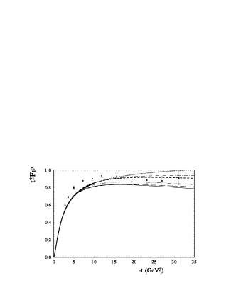
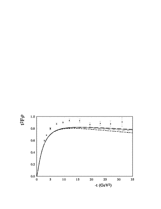
Figure 1: Proton Dirac form factor multiplied by $t^{2}$ in (a) top panel, the basic variant I Eq.(26) and (b) bottom panel, the variant IV Eq.(27).

Table 3: The sum of $\chi^{2}$ for the different PDFs sets and with different number of the fitting parameters.

N	Model	$\chi^{2}_{0}$	$\chi^{2}_{+1p}$	$\chi^{2}_{+1p}$	$\chi^{2}_{+2p}$	$\chi^{2}_{+3p}$	$\chi^{2}_{+4p}$
1	ABKM09	984	984	953	936	903	872
2a	JR08a	$1119$	861	891	861	860	857
2b	JR08b	$1242$	1242	880	868	868	864
3	ABM12	$1036$	1033	1031	1020	919	904
4a	KKT12a 8	$1170$	1133	1170	1108	934	888
4b	KKT12b	$1074$	1074	1064	1064	1036	988
5a	GJR07d	$1772$	1042	1553	936	884	878
5b	GJR07b	$1172$	1078	992	947	887	865
5c	GJR07a	$1215$	1214	1079	1024	940	894
5d	GJR07c	$8423$	1230	7279	1042	954	891
6a	MRST02	$1089$	1041	1035	1013	932	905
6b	MRST01	$1167$	1002	1129	999	898	873
7a	GP08a	$2189$	1575	1495	1017	886	879
7b	GP08b	$1423$	1382	1009	988	891	888
7c	GP08c	$1278$	1226	991	974	898	892
7d	GP08d	$4587$	2484	4575	3483	2388	2388
8a	MRST09a	$1785$	1184	1598	1107	974	887
8b	MRST09b	$1382$	1226	1149	1052	972	894
8c	MRST09c	$1260$	1168	1005	960	930	881
9	MR02P	$1344$	1187	1120	1044	946	875
10a	O12a	$1523$	1458	1080	1054	1007	932
10b	O12am	$1534$	1468	1077	1050	1007	932
10c	O12b	$1377$	1361	1134	1127	1052	958
10d	O12c	$1366$	1359	1192	1191	1085	981
11	MRST02R4	$2360$	2358	1879	1819	1786	1780

We analyzed the PDF sets in five cases: first, with minimum free parameters and flavor independence $f(x,t)$ Eq.(26) (basic variant), as was made in ST-PRDGPD , and then with an increase in the number of free parameters (a) free $p_{1}$ (both $u$ and $d$ quarks have the same power), (b) fixed $p_{1}$ and made as free $z_{1}$ (the $u$ quarks correspond to the basic variant and $d$ quark has the free power dependence), (c) made free $p_{1}$ and $z_{1}$ (both quarks have the independent power dependence), (d) using free $p_{1}$, $z_{1}$ and $z_{2}$ (the slopes of the $u$ and $d$ quarks can be different). The last two variants already have a small difference in $\chi^{2}$ for most variants of PDFs, as can be seen in Table 3 ( Coulomb 6 and 7). So including extra free parameters leads to small decreasing of $\chi^{2}$ and does not give new information about the properties of PDFs. We research also the case with the supplementary term of $x$ in $f(x)$ in the form $z_{3}\ x\ (1-x)$. The results are shown in the last column of Table 3. We can see that this variant does not give additional useful information about the PDF sets.

The PDF sets were taken as $24$ variants in different works with taking into account the leading order (LO), next leading order (NLO) and next-next leading order NNLO) in $\alpha_{s}$ of QCD (Table 1). The experimental data on the electromagnetic form factors were represented by $446$ experimental points.

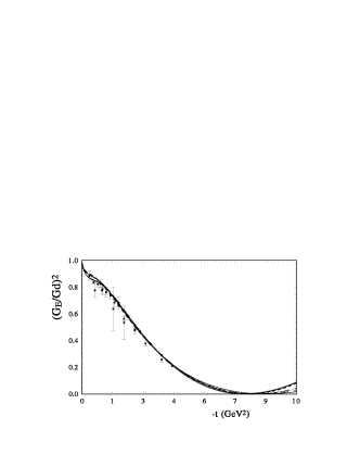
Figure 2: Proton $(G_{E}/Gd)^{2}$ in (a) top panel, the basic variant I Eq.(26) and (b) bottom panel, the variant IV Eq.(27). The data for $F_{1}^{p}$ are from Sill93 .

The whole sets of the experimental data are presented in Table 2. We include both compilations of the experimental data Andivadis94 and Arrington07 . The sets of the data have various corrections and the different methods taking into account the systematical errors. So we take into account only the statistical errors. Of course, we obtain sufficiently large $\sum\chi^{2}_{i}$. However, we are interested in the difference between $\chi^{2}$ obtained with the different PDF sets and the number of free parameters.

Table 4: Basic parameters of the model with the different PDFs sets

N	$p_{1}$	$p_{2}$	$\alpha_{H}$	$\alpha_{E}$	$x_{0}$	$e_{u}$	$e_{d}$
	fixed	$\pm 0.005$	$\pm 0.004$	$\pm 0.003$	$\pm 0.004$	$\pm 0.05$	$\pm 0.05$
1	2.0	0.507	0.377	$0.382$	$0.007$	2.69	0.09
2a	2.0	0.382	0.641	$0.735$	$0.001$	1.47	-0.53
2b	2.0	0.428	0.487	$0.567$	$0.004$	1.69	-0.55
3	2.0	0.510	0.377	$0.370$	$0.008$	2.86	0.24
4a	2.0	0.433	0.491	$0.479$	$0.008$	2.26	-0.04
4b	2.0	0.422	0.495	$0.508$	$0.008$	1.97	-0.04
5a	2.0	0.238	0.849	$0.837$	$0.000$	1.87	0.12
5b	2.0	0.342	0.683	$0.716$	$0.003$	1.79	-0.09
5c	2.0	0.415	0.498	$0.508$	$0.010$	2.29	0.09
5d	2.0	0.140	0.974	$1.019$	$0.000$	1.49	-0.23
6a	2.0	0.421	0.565	$0.550$	$0.005$	2.24	0.21
6b	2.0	0.392	0.596	$0.576$	$0.004$	2.20	0.21
7a	2.0	0.328	0.694	$0.878$	$0.007$	1.13	-0.99
7b	2.0	0.355	0.525	$0.657$	$0.006$	1.21	-1.12
7c	2.0	0.315	0.547	$0.662$	$0.003$	1.27	-0.97
7d	2.0	0.449	0.763	$0.635$	$0.000$	1.60	0.59
8a	2.0	0.218	0.776	$0.841$	$0.000$	1.46	-0.38
8b	2.0	0.326	0.632	$0.710$	$0.002$	1.54	-0.43
8c	2.0	0.357	0.600	$0.681$	$0.003$	1.56	-0.46
9	2.0	0.389	0.528	$0.561$	$0.002$	2.05	-0.11
10a	2.0	0.377	0.533	$0.615$	$0.001$	1.71	-0.44
10b	2.0	0.378	0.533	$0.613$	$0.001$	1.73	-0.44
10c	2.0	0.377	0.539	$0.628$	$0.000$	1.43	-0.61
10c	2.0	0.384	0.536	$0.619$	$0.000$	1.41	-0.60
11	2.0	0.388	0.579	$0.610$	$0.002$	1.52fix	0.31fix

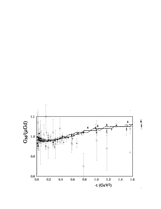
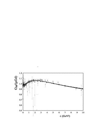
Figure 3: Proton $G_{M}/(\mu Gd)$ in (a) top and middle panels, the basic variant I Eq.(26) and (b) bottom panel, the variant IV Eq.(27).

Table 5: The fitting parameters of the GPDs with flavor dependence)

N	Model	$p_{1}$	$p_{2}$	$\alpha_{H}$	$\alpha_{E}$	$e_{u}$	$e_{d}$	$x_{0}$	$z_{1}$	$z_{2}$
		$\pm 0.02$	$\pm 0.01$	$\pm 0.01$	$\pm 0.03$	$\pm 0.07$	$\pm 0.05$	$\pm 0.002$	$\pm 0.03$	$\pm 0.03$
1	ABKM09	2.11	0.42	$0.45$	$0.57$	$0.67$	-1.88	0.004	$0.57$	$0.91$
2a	JR08a	1.93	0.42	0.62	$0.75$	$0.74$	$-1.37$	$0.006$	$0.76$	$0.98$
2b	JR08b	2.05	0.40	0.54	$0.67$	$0.71$	$-1.68$	$0.004$	$0.71$	$1.00$
3	ABM12	2.13	0.406	0.47	$0.61$	$0.55$	$-2.06$	$0.002$	$0.49$	$0.87$
4a	GJR07d	2.05	0.35	0.57	$0.74$	$0.47$	$-1.85$	$0.006$	$0.55$	$0.89$
4b	GJR07b	1.90	0.38	0.65	$0.80$	$0.62$	$-1.37$	$0.009$	$0.66$	$0.91$
4c	GJR07a	1.48	0.35	0.60	$0.78$	$0.32$	$-1.43$	$0.007$	$0.58$	$0.91$
4d	GJR07c	1.81	0.29	0.75	$0.89$	$0.67$	$-1.06$	$0.002$	$0.67$	$0.90$
5a	Kh-12a	1.97	0.40	0.52	$0.68$	$0.44$	$-2.00$	$0.007$	$0.51$	$0.83$
5b	Kh-12b	2.00	0.40	0.51	$0.58$	$1.38$	$-0.42$	$0.005$	$0.91$	$0.96$
6a	MRST02	1.94	0.42	0.57	$0.68$	$0.82$	$-1.20$	$0.006$	$0.63$	$0.88$
6b	MRST01	1.87	0.43	0.56	$0.68$	$0.71$	$-1.28$	$0.01$	$0.58$	$0.86$
7a	GP08a	1.74	0.58	0.51	$0.53$	$1.43$	$-0.49$	$0.04$	$1.05$	$1.21$
7b	GP08b	1.99	0.39	0.52	$0.56$	$1.47$	$-0.75$	$0.008$	$1.03$	$1.17$
7c	GP08c	1.98	0.35	0.53	$0.57$	$1.48$	$-0.69$	$0.005$	$1.02$	$1.13$
7d	GP08d	1.66	0.54	0.56	$0.73$	$0.12$	$-1.82$	$0.00$	$0.51$	$0.71$
8a	MRST09A	1.80	0.28	0.67	$0.88$	$0.34$	$-1.70$	$0.002$	$0.64$	$0.90$
8b	MRST09B	1.85	0.40	0.57	$0.75$	$0.35$	$-1.88$	$0.009$	$0.63$	$0.92$
8c	MRST09C	1.89	0.41	0.57	$0.73$	$0.46$	$-1.77$	$0.01$	$0.66$	$0.94$
9	MR02P	1.87	0.43	0.50	$0.65$	$0.46$	$-1.81$	$0.008$	$0.55$	$0.90$
10a	O12A	1.92	0.40	0.53	$0.71$	$0.27$	$-2.18$	$0.003$	$0.59$	$0.94$
10b	O12Am	1.92	0.40	0.53	$0.72$	$0.27$	$-2.19$	$0.003$	$0.59$	$0.94$
10c	O12C	1.94	0.39	0.54	$0.74$	$0.26$	$-2.26$	$0.001$	$0.63$	$0.92$
10c	O12D	1.97	0.37	0.55	$0.76$	$0.26$	$-2.26$	$0.00$	$0.64$	$0.91$
11	MRST02R4	1.88	0.48	0.51	$0.51$	$1.52$	$0.31fix$	$0.001$	$0.86$	$0.97$

In the final variant, most of the PDF sets gave approximately the same $\chi^{2}$ (Table 3). On this background of PDFs, one variant of GP08d GP08 and all variants of O12 CJ12 are essentially different and have large $\chi^{2}$. In the last row of Table 3, we show the calculation of the MRST02 MRST02 with the fixed parameters used by R04 and by us ST-PRDGPD . In this case $\chi^{2}$, is two times larger, but, on the whole, it confirms our qualitative model. The best descriptions were obtained with the PDF sets ABKM09 ABKM09 and JR08 JR08 . In this case, all 6 variants of the $t$ dependence gave a very close size of $\chi^{2}$. Also, we obtained a good description with the PDF sets ABM12 ABM12 and KKT12 KKT12 . It is interesting to note that the good result was obtained with the sufficiently old PDF sets MRST02 MRST02 and MRST01 MRST01 .

In most part, the best descriptions of the electromagnetic nucleon form factors were given by PDFs with the non-power forms of $g_{1}^{q}(x)$ eqs.(35)-(37). However, the PDFs JR08 used the standard form of the $g_{1}^{q}(x)$ though with free power of $x$, Eq.(34), instead of the standard $\sqrt{x}$.

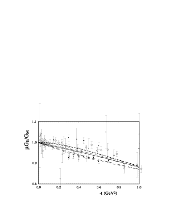
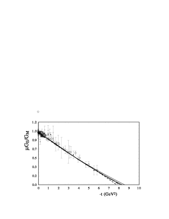
Figure 4: Proton $\mu G_{E}/G_{M}$ in (a) top and middle panels, the basic variant I Eq.(26) and (b) bottom panel, the variant IV Eq.(27).

The impact of the difference forms of PDFs will be seen, maybe, in the description of the separate form factors. It is worth noting, that the different PDF sets gave the similar descriptions in the proton form factors and a large difference in the description of the neutron form factors (see Fig.2, Fig.3, Fig.4 for the proton case and Fig. 6 , Fig. 7 for the neutron case). Probably, just the neutron data, in most part, lead to an essentially better description of the polarization data on the electromagnetic form factors.

In our qualitative model we showed that the descriptions of the experimental data, related with the Rosenbluth and polarization methods, can be obtained by changing the slopes of the $t$ dependence of the $u$ and $d$ quarks. In the present analysis all PDF sets led to the polarization case. Some difference was obtained only at large momentum transfer.

In Table 4, the values of the parameters of the basic variant are presented. Except some separate PDF sets, the slopes of $H$ and $E$ have the mean value $0.55$ and $0.6$, respectively. As shown in our previous work ST-PRDGPD , it is related with the Polarization variant of the obtained form factors. The Rosenbluth variant requires a large difference in these slopes. The value of the power $x$ in $f_{q}(x)$ equals approximately $0.4$. We can see that the difference of PDFs incoming in $E$ is distinguished, in most part, by the form of $u$-quark. It has the additional factor $(1-x)^{e_{u}}$ with $e_{u}\sim 2$. Some PDF sets gave the large $\chi^{2}$, especially one variant of GJR07 GJR07 and one variant of GP08 GP08 . If in last case we think it is the result of the Log-Log approximation; in the case of GJR07 it is, maybe, the result of some misprint of the printed parameters.

The number of the parameters of the variant IV (with 4 additional free parameters) is given in Table 5. If in the previous case the power of $(1-x)$ in $f(x)$ was fixed by $p_{1}=2$, now its value does not go out far. The arithmetic mean value over all 24 variants of PDFs $\bar{p}_{1}=1.91$. In the best variants it is slightly above $2$. In some other case it is less but, very likely, it reflects some attempt to improve the $x$ dependence of PDFs. The power of $x$ has arithmetic mean value $\bar{p}_{2}=0.39$. It coincides with the value in the previous (basic) case. The arithmetic mean of the slopes of $H$ and $E$ is $0.58$ and $0.72$. It is slightly above the previous case but again they do not strongly differ from each other. The large difference between variants I and IV comes from $e_{u}$ and $e_{d}$. Now $e_{u}$ decreases essentially and $e_{d}$ increases in absolute value. The coefficient $z_{1}$, reflecting the flavor dependence of the power $x$, differs from unity. It is related with the exchange value of $e_{u}$ and $e_{d}$. However, the next flavor dependence $z_{2}$ , which reflects the flavor dependence of the slopes GPDs, rest, on the average, near unity. It is interesting that in the last variant Mrst02R4 with fixed $e_{u}$ and $e_{d}$ we obtained the values of both parameters $z_{1}$ and $z_{2}$ near unity.

In Fig.1, it can be seen that the basic variant with minimum free parameters leads to a better description of the $t$ dependence of the data of the Dirac form factor $F_{1}(t)$. In this case, PDFs CJ12a, which gave one of the worst $\chi^{2}$ in the descriptions of all experimental data, gave the best description of $F_{1}^{p}(t)$. Note that the data on Fig.1 are related to the Rosenbluth method. Hence, it is very likely that these data are in contradiction with other data.

The description of the electric form factor $G_{E}(t)$ is good in both variants (the basic (I) and with 4 additional free parameters (IV)) (see Fig.2). In this figure, we can see that the difference between PDFs occurs only in the region of $t\approx 0.5$ GeV² and $-t\sim 6\div 7$ GeV². The description of the magnetic form factor $G_{M}(t)$ is good in all variants, especially with 4 additional parameters in the whole region of momentum transfer (Fig. 3c). The basic variant also gave a good description at small $t$ ( Fig. 3a) and not a large difference at large $t$ (Fig. 3b). Note that the best PDF ABKM09 (the low curve of Fig.3b) gave the maximum slope of $G_{M}^{p}$ and GP08 PDFs gave the minimal slope (upper curve of Fig.3b). As the result, we can see that the ratio $R_{p}=\mu G{E}(t)/G_{M}(t)$ for the proton describes well all existing polarization data. Some difference occurs at small $t$ and $-t>6$ GeV² for the basic variant (I). Such a difference practically disappears for the (IV) variant (see Fig.4c). Note that the PDFs ABKM09 in the gave the medium result at small and large $t$ (Fig. 4a and Fig. 4b). The PDFs GP08 gave the minimal result at small and large $t$ and the maximal value was given the PDFs MRST09. In Fig. 5, we show the difference between variant I and IV for the ratio $R_{p}$ for the different PDFs. It confirms our $\chi^{2}$ results. It can be seen that the difference is small up to $-t=4$ GeV² for all PDFs, especially for ABKM09 and MRST02. At large $t$ the difference grows fast especially for the PDF GP08 (upper curve on Fig. 5b) and PDFs O12 (low curve on Fig.5b).

For the neutron form factors, which were obtained with the same parameters as for the proton case using the isotopic symmetry, we obtained a larger difference for the PDF sets. Farther, we will show only the results for variant IV (with four additional free parameters). It should be noted that the experimental data for neutron form factors are obtained, in most part, from the deuteron or Helium target. It may lead to an increase in the uncertanty at large $t$, as we do not know exactly the wave functions of the light nuclei at large $t$.

The electric form factor of the neutron $G_{E}^{n}(t)$ describes well all PDFs, except GP08L and GP08c (upper curves on Fig. 6 ). At small $t$ the minimal values were given by PDFs O12C and maximal values PDFs ABKM09 which gave the medium value at large $t$. The magnetic form factor $G_{M}^{n}(t)$ has a larger difference for PDF (Fig.7). The large value is obtained with PDF GP08a and GP08c and minimal values with PDFs O12a and O12c. Hence, the ratio $R_{n}(t)=\mu_{n}G_{E}^{n}/G_{M}^{n}$ has a large difference already after $-t>2$ GeV² (Fig.8). The upper curves present the calculations with GP08a and GP08c. The lower curves correspond to the calculations with the PDFs O12c. As usual, in most part, the calculations with PDFs ABKM09 are in the mid-position. We see that the slope of the ratio $R_{n}(t)$ decreases at large $t$ for most PDF sets.

In Fig. 9, the ratio $R_{M}^{pn}(t)=\mu_{p}G_{M}^{n}(t)/(\mu_{n}G_{M}^{p}(t))$ is given. The ratio has a small difference for different PDFs up to $-t=2$ GeV² and then this difference grows. The decreasing ratio with $t$ is less for the PDFs GP08a and GP08c and larger for PDFs O12a and O12c.

The $t$ dependence of the Dirac and Pauli form factors of the proton and neutron are shown in Fig. 10. The Dirac form factor has the same slope at large $t$ for the proton and neutron cases and for different PDF sets (Fig.10a). All PDF sets lead to approximately the same $t$ dependence for the proton Pauli form factor up to large $t\sim 15$ GeV². The neutron Pauli form factors decrease slightly faster and have a wider region for different PDF sets. The faster decreasing is due to PDFs O12A and O12C, and low decreasing is given by PDFs MRST02.

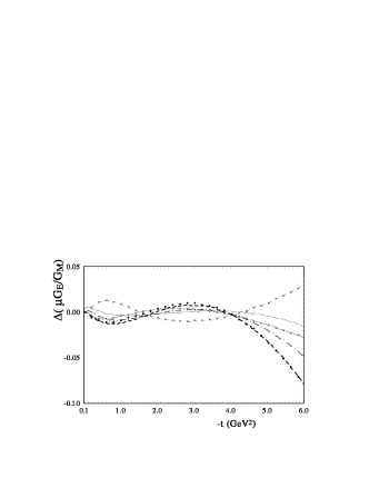
Figure 5: Difference between the basic variant I Eq.(26) and variant IV Eq.(27) of the ratio $R$.

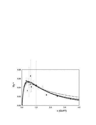
Figure 6: Neutron $G_{E}^{n}(t)$.

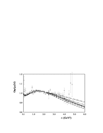
Figure 7: Neutron $G_{M}^{n}/(\mu_{n}Gd)$.

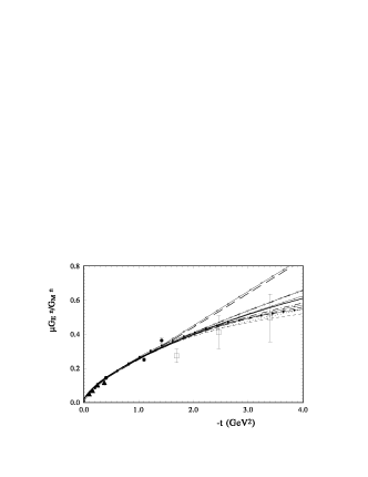
Figure 8: Neutron $R_{n}(t)=\mu_{n}G_{E}^{n}(t)/G_{M}^{n}(t)$.

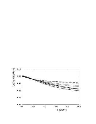
Figure 9: Ratio $R_{M}^{pn}=\mu_{p}G_{M}^{n}/(\mu_{n}G_{M}^{p})$.

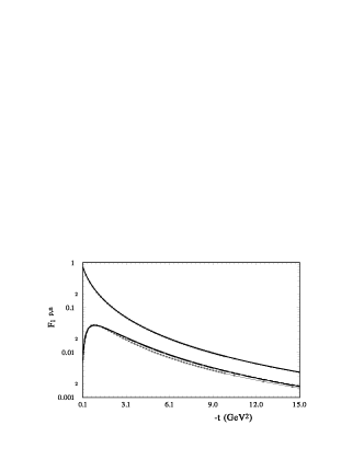
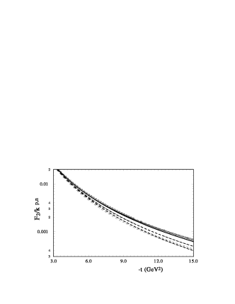
Figure 10: a) (top panel) Proton and neutron Dirac form factors $F^{p,n}_{1}$; b) (bottom panel) Proton and neutron Pauly form factors $F^{p,n}_{2}/k_{p,n}$.

V Flavor dependence of GPDs

Let us examine separate contributions of the $u$ and $d$ quarks to the electromagnetic form factors in our model of the $t$-dependence of GPDs. In the basic variant I, all flavor dependence comes only from the difference of the coefficients $e_{u}$ and $e_{d}$, Eq.(29), in PDFs incoming in $E(x,t)$. The coefficient $e_{d}$ is small and changing near zero for most PDFs. In these cases PDFs sets used non-power forms of $g_{2}^{q}(x)$. The PDFs, which used the standard Eq.(32) and Eq.(33), have the large negative size of $e_{d}$ and lead to the large $\chi^{2}$. The coefficient $e_{u}$ in this case is positive and large $1.5<e_{u}<2.5$. Hence, the $d$-distribution in $E(x,t)$ is, in most part, approximately the same as the $d$-distribution in $H(x,t)$. In the case of the additional free parameters (case IV, Table 5), the the coefficient $e_{d}$ increases up to $-2$ but the coefficient $e_{u}$ decreases and has positive values. In this case, we include the parameters which take into account the flavor difference $z^{d}_{1}$ and $z^{d}_{2}$ of GPDs, Eq.(27). The value of $z^{d}_{1}$ changes the behavior of the $d$ quark $(1-x)^{p_{1}z^{d}_{1}}$. So its size heavily depends on the $x$-dependence of PDFs. However, the difference in the slope of the $u$ and $d$ quarks is small. The coefficient $z^{d}_{2}$ near $1\pm 0.1$ is mostly of PDFs. It is very likely that the change of the coefficient reflects the problems of minimization of $\chi^{2}$ only.

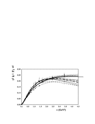
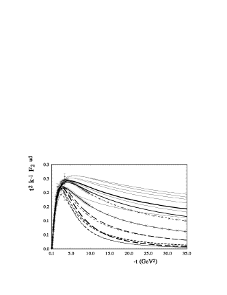
Figure 11: The $t$ dependence of $t^{2}F^{u,d}_{2}/k_{u,d}$ of the $u$ and $d$ quarks contributions at small $t$ (top) and at large $t$ (bottom panel).

In Fig.11, the obtained $t$ dependence of $t^{2}\mu_{u,d}F^{u,d}_{2}(t)$ of the $u$ and $d$ quark contributions to the form factors at small $t$ (Fig. 11a) and at large $t$ (Fig.11b) are presented. The dashed lines on these figures reproduce the $d$ quark contribution and the hard lines reproduce the $u$ quark contribution. The contribution of the $d$ quark exceeds the contribution of the $u$ quark up to $-t=2.5$ GeV² ( Fig. 11a). At larger momentum transfer the contribution of the $u$ quark exceeds the contribution of the $d$ quark, except the two cases of PDFs. First, an essentially different picture is given by PDFs GP08a. In this case, the contribution of the $d$ quark exceeds the contribution of the $u$ quark in the whole region of momentum transfer (upper dashed line with mark (x) for the $d$ quark and the low hard line with marks (x) for the $u$ quark in Fig. 11). For PDFs MRST02 the contribution of the $u$ quark has the minimum value, compared with others, at $-t=2$ GeV² and exceeds the $d$ quark contribution only after $-t=20$ GeV². The minimum $d$ contribution is obtained with PDFs O12 and MRST09a (low dashed curves in Fig. 11b ). Close to these cases PDFs ABKM09 give the $d$ contribution (thick long dashed curve in Fig. 11b). In all cases, we see the same behavior of the $u$ and $d$ quark contribution at large momentum transfer. The slopes of all curves are practically the same.

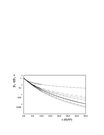
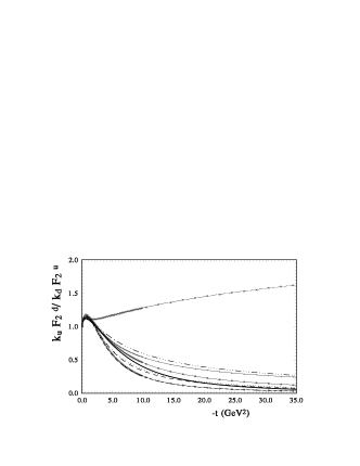
Figure 12: The ratio of the $u$ and $d$ quarks form factors $F_{1}(t)$ (top) and $F_{2}(t)$ (bottom panel) at large momentum transfer.

We obtain a remarkable picture for the ratio of the contributions of the $u$ and $d$ quarks to Dirac and Pauli form factors (Fig. 12). Again, we see a very different behavior for PDFs GP08a (upper lines in Fig. 12a and 12b). Other PDFs give a similar behavior. The PDFs O12 and MRST09a (low dashed curves in Fig. 12a,b) give the fastest decrease, and the PDFs JR08 and GJR07 less decrease in the ratio of the $d$ and $u$ quarks. It is interesting that this ratio of the contributions of the $u$ and $d$ quarks to the Dirac and Pauli form factors has the same relative behavior of the different PDFs. The order of the curves practically repeats the Dirac and Pauli form factors. Of course, the ratio for the Pauli form factor less decreases at large momentum transfer than the ratio for the Dirac form factor.

VI Gravitational form factors

Taking the matrix elements of energy-momentum tensor $T_{\mu\nu}$ instead of the electromagnetic current $J^{\mu}$ Pagels ; Ji97 ; PolyakovEMT

$$\left\langle p^{\prime}|\hat{T}^{Q,G}_{\mu\nu}(0)|p\right\rangle = \bar{u}(p^{\prime})\biggl{[}A^{Q,G}(t)\frac{\gamma_{mu}P_{\nu}}{2}$$

$$+ B^{Q,G}(t)\frac{i\left(P_{\mu}\sigma_{\nu\rho}+P_{\nu}\sigma_{\mu\rho}\right)\Delta^{\rho}}{4M_{N}}$$

$$+ \ C^{Q.G}(t)\frac{\Delta_{\mu}\Delta_{\nu}-g_{\mu\nu}\Delta^{2}}{M_{N}}\biggr{]}{u}(p)$$

one can obtain the gravitational form factors of quarks which are related to the second moments of GPDs

$$\int^{1}_{-1}dx\ x[H_{q}(x,\Delta^{2},\xi)=A^{q}_{2,0}(\Delta^{2})+(-2\xi)^{2}C^{q}_{2,0}(\Delta^{2}),$$

$$\int^{1}_{-1}dx\ x[E_{q}(x,\Delta^{2},\xi)=B^{q}_{2,0}(\Delta^{2})-(-2\xi)^{2}C^{q}_{2,0}(\Delta^{2}).$$ (39)

For $\xi=0$ one has

$$\int^{1}_{0}dx\ x{\cal{H}}_{q}(x,t)=A_{q}(t);\,\ \int^{1}_{0}dx\ x{\cal{E}}_{q}(x,t)=B_{q}(t).$$ (40)

Our results for $A_{u+d}(t)$ are shown in Fig.13. Our GPDs with different PDFs lead to the same $t$ dependence of $A_{u+d}(t)$. At $t=0$ these contributions equal $A(t=0)\approx 0.45$.

The corresponding calculations for $B_{q}(t)$ are shown in Figs. 14. In this case, we have the difference at $t=0$ and some difference in the $t$ dependence already at small momentum transfer. The PDFs O12a give the large values (upper curve in Fig.14) and PDFs GP8NNL gave the lower values (low curve in Fig.14). Others concentrated in two clusters. One gave $B_{grav}(t=0)=-0.15$ (the PDFs JR8a, MRST09a, MRST09b, GJR07b, and second gave $B_{grav}(t=0)=-0.11$ the PDFs ABKM09, ABM12, KKT12A, MRST02. In our previous work ST-PRDGPD , we obtained $B_{grav}(t=0)=-0.05$ that is close to the zero value. That is a sort of compensation for the $u$ and $d$ quarks supporting the conjecture Teryaev-s3 ; Teryaev:2006fk about the validity of the Equivalence Principle separately for quarks and gluons.

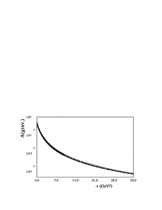
Figure 13: Gravimagnetic form factor $A(t)$.

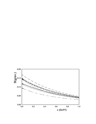
Figure 14: Gravimagnetic form factor $B(t)$.

Note that nonperturbative analysis within the framework of the lattice OCD indicates that the net quark contribution to the anomalous gravimagnetic moment $B_{u+d}(0)$ is close to zero Gockler04 ; Hagler05 . Now, our results contradict this conclusion. Probably, it points out the important contribution of the gluon part.

VII The Compton cross sections

The processes of the wide angle Compton scattering $\gamma^{*}p\rightarrow\gamma p$ gave the possibility to study the complicated hadronic dynamics in hard exclusive processes KivVan-13 . There are two processes - the deeply virtual Compton scattering (DVCS) (in this case the initial photon is highly virtual while the final photon is real and the effective masses of photons are different) and the real Compton scattering (RCS) (with both photons being real and equal). Large virtuality of the initial photon is sufficient for making the handbag diagram dominant R97 ; JiOs97 . The GPDs in this case have the large dependence on $\xi$. In the case of the RCS the GPDs have $\xi=0$. Hence, we can use our ansatz for the $t$ and $x$ dependence of the GPDs and calculate the corresponding cross sections.

Our calculations are based on the works R98 ; 104 and Kroll13 . The differential cross section for that reaction can be written as

$$\frac{d\sigma}{dt}=\frac{\pi\alpha^{2}_{em}}{s^{2}}\frac{(s-u)^{2}}{-us} [ R_{V}^{2}(t)\ -\ \frac{t}{4m^{2}}R^{2}_{T}(t)$$

$$+ \frac{t^{2}}{(s-u)^{2}}R^{2}_{A}(t)],$$

where $R_{V}((t)$, $R_{T}(t)$, $R_{A}(t)$ are the form factors given by the $1/x$ moments of corresponding GPDs $H^{q}(x,t)$, $E^{q}(x,t)$, $\tilde{H}^{q}(x,t)$ . The last is related with the axial form factors. As noted in Kroll13 , this factorization, which bears some similarity to the handbag factorization of DVCS, is formulated in a symmetric frame where the skewness $\xi=0$. For $H^{q}(x,t)$, $E^{q}(x,t)$ we used the PDFs obtained from the works JR08 ; KKT12 ; ABKM09 ; ABM12 with the parameters are presented in Table 5, obtained in our fitting procedure of the description of proton and neutron electromagnetic form factors. For $\tilde{H}^{q}(x,t)$ we take $\Delta q$ in the form

$$x\Delta q=N_{i}x^{a}_{1}(1+a_{2}\sqrt{x}+a_{3}x),$$ (42)

with the parameters are determined in 80 . Our calculations of $R_{i}$ on the whole, correspond the calculations Kroll13 , but the integrals with our Ansatz of the $t$ dependence of GPDs do not divergence at momentum transfer $-t>2$ GeV². In the work Kroll13 they presented $R_{i}$ beginning from $-t=4$ GeV². Note that the last term in Eq.(VII) has the small coefficient and its impact on the differential cross sections of RCS is very small (from 2$\%$ at small $t$ and up to $10\%$ at large momentum transfer). It is essentially less than theoretical indeterminacy.

Our calculations of the differential cross sections of RCS are shown in Fig.15 at three energies $s=9.8,10.92$ and $20$. Obviously, the calculations have sufficiently good coincidence with the existing experimental data and in whole coincides with calculations Kroll13 . The behavior of the experimental data at $s=9.8$ GeV² and large $t$ is probably connected with the kinematical property when $-t\rightarrow s$. Probably, it is necessary to take into account the next NLO terms KivVan-13 .

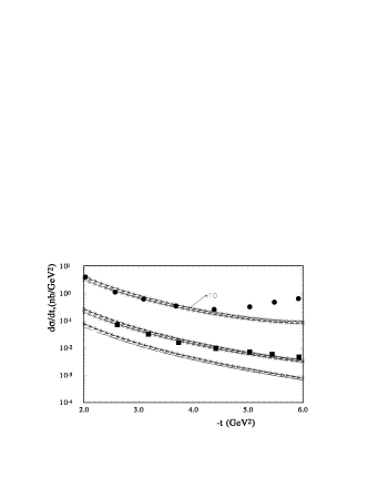
Figure 15: Differential Compton cross sections $\gamma p\rightarrow\gamma p$; the curves are our calculations at $s=8.9$ GeV² ( with factor $10$), $s=10.92$ GeV², and $s=20$ GeV² ( hard line, dashed line, dot-dashed line with (x), med-dashed line with ($+$), correspond to the PDFs [50,52,53,48]; the data points 105 are for $s=8.9$ GeV² (circles with factor $10$); $s=10.92$ GeV² (squares).

VIII Conclusions

The complex analysis of the corresponding description of the electromagnetic form factors of the proton and neutron by the different PDF sets (24 cases) was carried out . These PDFs include the leading order (LO), next leading order (NLO) and next-next leading order (NNLO) determination of the parton distribution functions. They used the different forms of the $x$ dependence of PDFs, eqs. (31 - 37). The analysis was carried out with different forms of the $t$ dependence of GPDs. The minimum number of free parameters was six and maximum were ten. We found that the best description was given by PDFs ABKM09 . In this case, the increase in the number of the free parameters leads to a small decrease in $\chi^{2}$. It means that the $x$ dependence of PDFs corresponds sufficiently well to the $u$ and $d$ distributions in the nucleon to reproduce the electromagnetic form factors. Note that these PDFs used the special power $x$ dependence of PDFs. The other PDFs JR08 ; ABM12 ; KKT12 ; GJR07 ; MRST02 also a similar behavior as ABKM09 and have a small change in $\chi^{2}$ with increasing number of the free parameters and lead to good descriptions with minimum free parameters. Note, it is remarkable that old PDFs MRST02 are in this list too. Practically in all our calculations PDFs ABKM09 gave the medium result between other PDFs. This confirms the result the minimum of $\chi^{2}$ obtained with the minimum of number of free parameters. We did not find a visible difference between PDFs with a different order. This is in accord with the conclusion of paper Forte13NLO that the theoretical uncertainty of PDFs exceeds the uncertainty of the perturbative series.

In the final analyses, we found that all PDFs in the simultaneous description of the proton and neutron electromagnetic form factors led to the ”polarization” case of the $t$-dependence of the form factors.

The flavor dependence in these cases, in most part, comes from the spin dependence part of PDFs. We obtained good descriptions of the electric and magnetic form factors of the proton and neutron simultaneously. We found that different PDFs gave almost the same descriptions of the proton form factors at small momentum transfer. The difference appears only at large $t$. Our calculations of the $u$ and $d$ quark contributions show the same $t$ dependence at large $t$.

All PDFs gave approximately the same size and the $t$-dependence of the gravitation form factors $A(t)$ as the second moment of the GPDs. The size of the gravimagnetic form factor $B(t=0)$ differs from zero. The PDFs ABKM09 gave $B_{grav.}(t=0)=-0.12$. It is above the result obtained by us in the qualitative description of the nucleon form factor ST-PRDGPD which was $B_{grav.}(t=0)=-0.05$. Hence, this may indicate on the important contribution of the gluon part.

References

- (1) E.L. Lomon, S. Pacetty, Phys.Rev. D 86 039901 (2012).
- (2) L.L. Foldy, Phys.Rev. 87 688 (1952).
- (3) I.A. Qattan and J. Arrington, Phys.Rev. C86 065210 ( 2012).
- (4) F.J. Ernst, R.G. Sachs, and K.C. Wali Phys. Rev. 119 1105 (1960).
- (5) R.G. Sachs, Phys.Rev. 126 2256 (1962).
- (6) J.J. Kelly, Phys.Rev. C66 065203 (2002).
- (7) M.N. Rosenbluth, Phys.Rev.79 615 (1950).
- (8) A.I. Akhiezer and M.P. Rekalo Sov.J.Nucl.Phys. 3 277 (1974).
- (9) R.G. Arnold, C.E. Carlson, and F. Gross, Phys.Rev. C 23 363 (1981).
- (10) P.A.M. Guichon, M. Vanderhaeghen, Phys.Rev,Lett. 91 142303-1 (2003). P.G. Blunden, W. Melnitchouk, A. Tjon, Phys.Rev,Lett. 91, 142304-1 (2003); Chen Y.C., et al., Phys.Rev.Lett. 93, 122301-1 (2004); M. P. Recalo, E. Tomasi-Gustafssn, Eur.Phys.J. A22 (204) 331; S. Dubnichka, E. Kuraev, M. Secansky, A. Vinnikov, hep-ph/0507242.
- (11) Yu.M. Bystritsky, E.A. Kuraev, and E. Tomasi-Gustafsson, arXiv:hep-ph/0603132.
- (12) E.A. Kuraev, V.V. Bytev, Yu.M. Bystritskiy, and E. Tomasi-Gustafsson, Phys.Rev. D 74 013003 (2006).
- (13) I. A. Qattan, et al., Phys.Rev.Lett. 94 142301 (2005).
- (14) G.D. Gates et al., Phys.Rev.Lett., 106 252003 (2011).
- (15) D. Muller, D. Robaschik, B. Geyer, F.M. Dittes and J. Horejsi, Fortsch. Phys. 42, 101 (1994).
- (16) Ji X.D. Phys. Lett., B. 78 610 (1997); Ji X.D., Phys. Rev. D55,7114 (1997).
- (17) Radyushkin A.V., Phys. Rev., D56, 5524 (1997).
- (18) A. V. Radyushkin, Phys. Rev. D58 114008 (1998).
- (19) M. Burkardt, Phys. Rev. D62 071503(R) (2000).
- (20) K. Kumericki and D. Muller, Nucl. Phys. B 841 1 (2010).
- (21) K. Kumericki et al. arXiv: [1105.0899].
- (22) M. Guidal, H. Moutarde, M. Vanderhaeghen, Rept.Prog.Phys. 76 066202 (2013).
- (23) K. Goeke, M.V. Polyakov, and M. Vanderhaeghen, Prog.Part.Nucl.Phys. 47, 401 (2001).
- (24) S. Boffi and B. Pasquini (0711.2625) Riv.Nuovo Cim. 30, 387 (2007).
- (25) M. Guidal, M.V. Polyakov, A.V. Radyushkin, and M. Vanderhaeghen, Phys. Rev. D 72 , 054013 (2005).
- (26) G.R. Goldstein, J.O. Hernandez, S. Liuti, Phys.Rev. D84 034007 (2011).
- (27) J.O. Gonsales-Hernandes et al., arXiv:1206.1876 v3.
- (28) M.Diehl et al., Eur.Phys. J. C 39, 1 (2005).
- (29) M.Diehl and P. Kroll, Eur.Phys. J. C 73, 1 (2013).
- (30) F. Yuan, Phys. Rev., D69, 051501(R) (2004).
- (31) I. V. Anikin et al. arxiv:1112.1849)
- (32) M. Guidal and H. Moutarge, Eur. Phys.J. A42,71 (2009).
- (33) M. Guidal, Phys.Lett. B bf 689 156 (2010).
- (34) Fiore R., et al., Mod.Phys., A24, 2551 (2009).
- (35) G. Antchev G. et al. (TOTEM Coll.), arXiv: 1110.1395.
- (36) The TOTEM Collaboration (G. Antchev et al.) EPL, 95, 41001 (2011).
- (37) H. Miettinen , Nucl.Phys. B166, 365 (1980).
- (38) S. Sanielevici, P. Valin, Phys.Rev. D29, 52 (1984).
- (39) O.V. Selyugin, Eur.Phys.J. C72, 2073 (2012).
- (40) A.D. Martin et al., Phys. Lett. B 531 216 (2002).
- (41) Selyugin O.V., Teryaev O.V., Phys. Rev. D79, 033003 (2008).
- (42) M. Burkardt , Phys.Lett. B 595, 245 (2004).
- (43) A.D. Martin, R.G. Roberts, W.J. Stirling, and G. Watt, Eur.Phys.J., C 63, 189 (2009).
- (44) A.D. Martin, R.G. Roberts, W.J. Stirling, and R.S. Thorne, Eur.Phys.J., C 23, 73 (2002).
- (45) J. F. Owens, A. Accardi, W. Melnitchouk, Phys.Rev., D 87, 094012 (2013).
- (46) M. Gluck, Phys.Rev., D 79 , 074023 (2009).
- (47) M. Gluck, C. Pisano, and E. Reya, Phys.Rev., D 77 , 074002 (2008); 78 019902(E) (2008).
- (48) H. Khanpour et al., arXiv:1205.5194
- (49) J. Pumplin, et al., JHEP 0207:012 (2002).
- (50) S. Alekhin et al., Phys.Rev. D81 , 014032 (2010);
- (51) S. Alekhin, J. Blu”mlein, and S. Moch, Phys.Rev. D86 , 054009 (2012).
- (52) M. Gluck, P. James-Delgado, E. Reya, Eur.Phys.J., C53 355 (2008).
- (53) L. Andivahis et al., Phys.Rev. D50 5491 (1994).
- (54) J. Arrington, W. Melnitchouk, J.A. Tjon, Phys.Rev., C76, 035205 (2007).
- (55) R.C. Walker et al., Phys.Rev. D49, 5671 (1994).
- (56) P.E. Boosted, et al., Phys.Rev.Lett. 68, 3841 (1992).
- (57) X. Zhan, et all., Phys.Lett., B705, 59 (2011).
- (58) G. Ron et al., Phys.Rev., C84, 055204 (2011).
- (59) F. Borkowski, et al., Nucl.Phys. B93, 461 (1975).
- (60) A.F. Sill, et al., Phys.Rev. D 48, 29 (1993).
- (61) W. Bartel Nucl.Phys., B58, 429 (1973).
- (62) C.B. Grawford, et al., Phys.Rev.Lett., 98 , 052301 (2007).
- (63) B.D. Milbrath, et al., Phys.Rev.Lett., 80 452(1998); Erratum-ibid 82 2221(1999).
- (64) M.K. Jones, et al., Phys.Rev., C 74, 034201, (2006).
- (65) O. Gayou, et al., Phys.Rev.Lett., 88 092301 (2002).
- (66) J. Bermuth, et al., Phys.Lett., B564, 199 (2003).
- (67) D.I. Glazier, et al., Eur.Phys.J. A24, 101 (2005).
- (68) R. Madey, et al., Phys.Rev.Lett., 91 122002 (2003).
- (69) S. Rock, Phys.Rev.Lett. 49 19 (1982).
- (70) P.R. Eden, Phys.Rev C50, R1749 (1994).
- (71) EPJ A6 J. Becker et al., Eur.Phys.Jour. A6, 329 1999.
- (72) H. Zhu, et al., Phys.Rev. Lett. 87 081801 (2001).
- (73) G. Warren, et al., Phys.Rev.Lett., 92 042301 (2004).
- (74) Rohe, Phys.Rev.Lett. 83, 4257 (1999).
- (75) G. Kubon, et al., Phys.Lett., B524, 26 (2002).
- (76) W.K. Brooks and J.D. Lanchniet, Nucl.Phys. A755, 261 (2005).
- (77) J. Lachniet et al., Phys.Rev.Lett. 102 19210 (2009).
- (78) P. Markowitz Phys.Rev. C 48, R5 (1993)
- (79) E.E.W. Bruins Phys.Rev.Lett. 75, 21 (1995).
- (80) S. Riordan, et al., Phys.Rev.Lett., 105, 262302 (2010).
- (81) H. Pagels Phys.Rev. 144, 1250 (1966).
- (82) K. Goeke, J. grabis, J. Ossmann, M.V. Polyakov, P. Schweitzer, A. Silva, and D. Urbano, Phys. Rev. D 75 , 094021 (2007).
- (83) O.V. Teryaev, Czech. J. Phys. 53 47A (2003).
- (84) O. V. Teryaev, AIP Conf. Proc. 915, 260 (2007).
- (85) M. Goeckeler, R. Horslay, D. Pleiter, P.E.L. Rakow, and G. Schierholz, Nucl.Phys. B, Proc.Suppl. 119, 398 (2003).
- (86) Ph. Hagler, J.W. Negele, D.B. Renner, W. Schroers, T. Lippert, and K. Schilling (LHPC Collaboration), Eur.Phys. J., A 24, 29 (2005).
- (87) N. Kivel and M. Vanderhaegen, arXiv:1312.5456.
- (88) X.D. Ji, J. Osborne, Phys. Rev. D 58, 094018 (1998).
- (89) M.Diehl, T. Feldmann, R. Jakob, and P. Kroll, Eur.Phys. J. C 8, 409 (1999).
- (90) D. de Florian, R. Sassot, m. Stratmann and W . Vogelsang, Phys. Rev. D 80, 034030 (2009).
- (91) A. Danagoulian et al. [Jeffferson Lab. Hall A Collaboration], Phys.Rev. Lett. 98 152001 (2007).
- (92) S. Forte, A. Isgro and Ch. Vita, arXiv: 1312.6688.