A multilevel stochastic collocation method
for partial differential equations with random input data
Abstract
Stochastic collocation methods for approximating the solution of partial differential equations with random input data (e.g., coefficients and forcing terms) suffer from the curse of dimensionality whereby increases in the stochastic dimension cause an explosion of the computational effort. We propose and analyze a multilevel version of the stochastic collocation method that, as is the case for multilevel Monte Carlo (MLMC) methods, uses hierarchies of spatial approximations to reduce the overall computational complexity. In addition, our proposed approach utilizes, for approximation in stochastic space, a sequence of multi-dimensional interpolants of increasing fidelity which can then be used for approximating statistics of the solution as well as for building high-order surrogates featuring faster convergence rates. A rigorous convergence and computational cost analysis of the new multilevel stochastic collocation method is provided, demonstrating its advantages compared to standard single-level stochastic collocation approximations as well as MLMC methods. Numerical results are provided that illustrate the theory and the effectiveness of the new multilevel method.
keywords:
multilevel methods, stochastic collocation, PDEs with random input data, sparse grids, uncertainty quantification, finite element methods, multivariate polynomial approximation, hierarchical methods, high-dimensional approximationAMS:
65C20, 65C30, 65N30, 65N35, 65M75, 65T50, 65T601 Introduction
Nowadays, mathematical modeling and computer simulations are used extensively in many scientific and engineering fields, usually with the goal of understanding or predicting the behavior of a system given its inputs such as the computational domain, model parameter values, and source terms. However, whether stemming from incomplete or inaccurate knowledge or from some inherent variability in the system, often these inputs may be subject to uncertainty. In order to correctly predict the behavior of the system, it is especially pertinent to understand and propagate the effect of the input uncertainty to the output of the simulation, i.e., to the solution of the mathematical model.
In this paper, we consider systems which are modeled by elliptic partial differential equations (PDEs) with random input data. We work under the finite-dimensional noise assumption, i.e., we assume that the random inputs are characterized by a finite-dimensional random vector. When enough information is available to completely characterize the randomness in the inputs, probability theory provides a natural setting for quantifying uncertainties. The object of our computations is the accurate calculation of solution of stochastic elliptic PDEs or statistics of some functional of the solution of the PDE. For instance, in addition to the solution itself, one might be interested in the expected value or variance of the solution in a given region of the computational domain.
A large number of methods have been developed for the numerical solution of PDEs with random inputs; see, e.g., [GWZ14] and the references cited therein. The most popular approach is the Monte Carlo (MC) methods which involves random sampling of the input vector of random variables (also referred to as the stochastic parameter space) and the solution of the deterministic PDE at each of the sample points. In addition to the benefits of simple implementation and a natural decoupling of the stochastic and spatial degrees of freedom, MC methods feature a convergence rate that is independent of the dimension of the stochastic space. This makes it particularly attractive for high-dimensional problems. However, the convergence is in general very slow and, especially in case the stochastic space is only of moderate dimension and the solution of the PDE or of a functional of interest is smooth, better convergence rates can be achieved using more sophisticated methods.
Stochastic collocation (SC) methods [1, 17, 18] are similar to MC methods in the sense that they involve only the solution of a sequence of deterministic PDEs at given sample points in the stochastic space. However, rather than randomly chosen samples, SC methods use a deterministic grid of points at which one then solves the corresponding deterministic PDE, and then builds an interpolant, either using global Lagrange-type polynomials [1, 17, 18] or even local hierarchical basis functions [GWZ13, Ma:2009p4298]. For problems where the solution is a smooth function of the random input variables and the dimension of the stochastic space is moderate, SC methods have been shown to converge much faster than MC methods.
Unfortunately, for most problems, stochastic collocation methods suffer from the curse of dimensionality, a phrase that refers to the deterioration of the convergence rate and the explosion of computational effort as the dimension of the stochastic space increases. In this paper, we introduce a multilevel stochastic collocation (MLSC) approach for reducing the computational cost incurred by standard, i.e., single level, SC methods. Drawing inspiration from multigrid solvers for linear equations, the main idea behind multilevel methods is to utilize a hierarchical sequence of spatial approximations to the underlying PDE model that are then combined with stochastic discretizations in such a way as to minimize computational cost. Starting with the pioneering works [15] in the field of integral equations and [12] in the field of computational finance, the multilevel approach has been successfully applied to many applications of MC methods; see, e.g., [2, 5, 8, 13, 11, 16]. The MLSC methods we consider in this paper are similar to the multilevel quadrature schemes studied in [14]. However, our focus is on the analysis of the computational complexity of the multilevel algorithms and also includes results for functionals of the solution. In particular, we prove new interpolation error bounds on functionals of the solution that are needed for the analysis of the MLSC methods.
The outline of the paper is as follows. In Section 2, we introduce the mathematical problem, the main notation used throughout, the assumptions on the parametrization of the random inputs that are used to transform the original stochastic problem into a deterministic parametric version, and needed assumptions about the regularity of the solution of the PDE. A description of the spatial and stochastic approximations as well as the formulation of the MLSC method follows in Section 3. In Section 4, we provide a general convergence and complexity analysis for the MLSC method. As an example of a specific single level SC approach satisfying our interpolation assumptions, we describe, in Section 5, a generalized sparse grid stochastic collocation approach based on global Lagrange interpolation. In Section 6, we provide numerical results that illustrate the theoretical results and complexity estimates and also explore issues related to the implementation of the MLSC method.
2 Problem Setting
Consider the problem of approximating the solution of an elliptic partial differential equation (PDE) with random input data. To this end, let , denote a bounded, Lipschitz domain with boundary denoted by and let denote a complete probability space. Here, denotes the set of outcomes, the -algebra of events, and a complete probability measure. Given random fields , the model problem we consider is stated as follows: find such that almost surely
| (1) |
We make the following assumptions on and :
-
A1.
(Finite-dimensional noise) The random fields and are determined by a finite number of random variables, denoted by the random vector .
-
A2.
(Boundedness) The image of is bounded for all and, with , the random variables have a joint probability density function , where denotes the one-dimensional PDF corresponding to the probability space of the random fields. Without loss of generality, we assume that .
Remark 1.
Another setting having a finite number of random variables is that of the coefficient and the forcing function depending on a a finite number of independent scalar random physical parameters, e.g., diffusivities, reaction rates, porosities, elastic moduli, etc. In this case, each of the parameters would have its own PDF , , so that the joint PDF is now given by . The algorithms discussed in this work all apply equally well to this setting.
Under assumptions A1 and A2, it follows from the Doob-Dynkin Lemma that the solution to (1) can also be characterized in terms of the random vector . The solution thus has a deterministic, parametric equivalent , with the probability space taking the place of ; see, e.g., [1]. Here, denotes the Borel -algebra generated by the open subsets of . In what follows, we will therefore denote the solution by for and . Then we also assume:
-
A3.
(Existence and uniqueness) The coefficients are uniformly bounded and coercive, i.e., there exists
and so that the problem (1) admits a unique solution with realizations in , i.e., almost surely.
Here, given a Banach space of functions on , the weighted Bochner spaces for are defined by
with corresponding norm given by
Assumption A1 is naturally satisfied by random fields that only depend on a finite set of parameters, e.g.,
and similarly for , where is a vector of independent random variables. If this is not the case, approximations of and that satisfy assumption A1 can be obtained by appropriately truncating a spectral expansion such as the Karhunen-Loève expansion [10]. This introduces an additional error; see [17] for a discussion of the effect of this error on the convergence of stochastic collocation methods and [9, 4] for bounds on the truncation error.
Assumption A2 can be weakened to include the case of unbounded random variables such as Gaussian variables. See [1] for an analysis of the interpolation error and note that, with only minor modifications, the multilevel stochastic collocation method introduced in this paper also applies to unbounded random variables. Furthermore, assumption A3 can be weakened to include coefficients that are not uniformly coercive; see [5, 19].
Finally, we remark that the multilevel stochastic collocation method proposed in this paper is not specific to the model problem (1); it can be applied also to higher-order PDEs and other types of boundary conditions.
3 Hierarchical multilevel stochastic collocation methods
We begin by recalling that standard stochastic collocation (SC) methods generally build an approximation of the solution by evaluating a spatial approximation at a given set of points in , where is a finite-dimensional subspace. In other words, we compute . Then, given a basis for the space , we use those samples to construct the fully discrete approximation given by the interpolant
| (2) |
where the coefficients are determined by the interpolating conditions for . In (2), we label the standard SC approximation by ‘SL’ to indicate that that approximation is constructed using a single set of points in stochastic space, in contrast to the multilevel approximations considered below that use a hierarchy of point sets; thus, we refer to (2) as a single level approximation. A wide range of choices for the interpolation points and basis functions are possible. A particular example of the approximation (2), namely global Lagrange interpolation on generalized sparse grids, is given in Section 5.
Convergence of the SC approximation (2) is often assessed in the natural -norm, and the goal is to determine a bound on the error . To obtain a good approximation with SC methods, it is necessary in general to use accurate spatial approximations and a large number of collocation points. To determine the coefficients of the interpolant (2), the method requires the computation of for so that, in practice, the cost can grow quickly with increasing . Therefore, to reduce the overall cost, we consider a multilevel version of SC methods that combines different levels of fidelity of both the spatial and parameter approximations.
3.1 Spatial approximation
For spatial approximation, we use hierarchical family of finite element discretizations [3, 6]. As discussed in [14], the formulation of the multilevel method does not depend on the specific spatial discretization scheme used and the results readily hold for other choices. For , define a hierarchy of nested finite element spaces
where each consists of continuous, piecewise polynomial functions on a shape regular triangulation of having maximum mesh spacing parameter . Note that merely serves to index the given spaces; the approximation properties of the space is governed by . For simplicity, we assume that the triangulations are generated by iterative uniform subdivisions of the initial triangulation ; this implies that for some , and that indeed the corresponding finite element spaces are nested.
Remark 2.
For simplicity, we have assumed that the finite element family of spaces is nested, and in fact, are constructed by a series of uniform subdivisions of a parent mesh with mesh size . Neither of these assumptions are necessary for our algorithms or conclusions to hold, provided for some and all ; in such cases, the finite element spaces are not necessarily nested.
We also let denote the Galerkin projection of onto , i.e., denotes the finite element approximation. Note that is still a function on the stochastic parameter space . We assume the following approximation property of the finite element spaces :
-
A4.
There exist positive constants and , independent of , such that for all ,
In general, the rate depends on the (spatial) regularity of , which in turn depends on the regularity of and as well as on the geometry of the domain . For example, if , , and are sufficiently regular so that , assumption A4 holds with and dependent only on and . For additional examples and detailed analyses of finite element errors, see [19].
3.2 Stochastic interpolation
For stochastic approximation, we use interpolation over , where we assume . The specific choice of interpolation scheme is not crucial at this juncture. We begin by letting denote a sequence of interpolation operators using points. We assume the following:
-
A5.
There exist positive constants , , and , and a Banach space containing the finite element approximations such that for all and all
for some function and a decreasing sequence that admit the estimates
Remark 3.
As in the previous section, is merely an index; we use the same index for the hierarchies of spatial and stochastic approximations because, in the multilevel SC method we introduce below, these two hierarchies are closely connected.
Remark 4.
determines the approximation properties of the interpolant. Moreover, we allow non-unique interpolation operators in the sequence, i.e., it is possible that, for any , and therefore and . Thus, although the spatial approximation improves with increasing , i.e., , we allow for the parameter space approximation for the index remaining the same as that for .
In Section 5, assumption A5 is shown to hold, with , for global Lagrange interpolation using generalized sparse grids. The bounds on the function in assumption A5 are shown to be the key to balancing spatial and stochastic discretizations through the multilevel formulation. Crucially, we make use of the fact that the interpolation error is proportional to the size of the function being interpolated, measured in an appropriate norm. In the case of the model problem (1), this norm is usually related to the (spatial) -norm. The bounds in assumption A5 then arise from the fact that for any , is bounded by a constant, independent of , whereas decays with for some . We usually have , where is as in assumption A4. Note that we have chosen to scale the bound on by to simplify calculations. Because is a constant, this does not affect the nature of the assumption.
3.3 Formulation of the multilevel method
As in the previous sections, denote by and sequences of spatial approximations and interpolation operators in parameter space, respectively. Then, for any , the formulation of the multilevel method begins with the simple telescoping identity
| (3) |
where, for simplicity, we set .
It follows from assumption A5 that as , less accurate interpolation operators are needed in order to estimate to achieve a required accuracy. We therefore define our multilevel interpolation approximation as
| (4) |
Rather than simply interpolating , this approximation uses different levels of interpolation on each difference of finite element approximations. To preserve convergence, the estimator uses the most accurate interpolation operator on the coarsest spatial approximation and the least accurate interpolation operator on the finest spatial approximation . Note that in (4) a single index is used to select appropriate spatial and stochastic approximations and thus these approximations are indeed closely related.
4 Analysis of the multilevel approximation
This section is devoted to proving the convergence of the multilevel approximation defined in Section 3.3 and analyzing its computational complexity. We first prove, in Section 4.1, a general error bound, whereas in Sections 4.2 and 4.3 we prove a bound on the computational complexity in the particular case of an algebraic decay of the interpolation errors.
4.1 Convergence analysis
We consider the convergence of the multilevel approximation to the true solution in the natural norm .
First, we use the triangle inequality to split the error into the sum of a spatial discretization error and a stochastic interpolation error, i.e.,
| (5) |
The aim is to prove that with the interpolation operators chosen appropriately, the stochastic interpolation error () of the multilevel approximation converges at the same rate as the spatial discretization error (), hence resulting in a convergence result for the total error.
For the spatial discretization error (), it follows immediately from assumption A4 that
4.2 Cost analysis
We now proceed to analyze the computational cost of the MLSC method. We consider the -cost of the estimator, denoted here by , which is the computational cost required to achieve a desired accuracy . In order to quantify this cost, we use the convergence rates of the spatial discretization error and, for the stochastic interpolation error, the rates given by assumptions A4 and A5. In particular, we will assume that A5 holds with for some .
Remark 5.
The choice best reflects approximations based on SC methods that employ sparse grids. In particular, as mentioned in Section 3.2, algebraic decay holds for the generalized sparse grid interpolation operators considered in Section 5; see Theorem 13. For other possible choices in the context of quadrature, see [14].
In general, the MLSC method involves solving, for each , the deterministic PDE for each of the sample points from ; in fact, according to (4), two solves are needed, one for each of two spatial grid levels. Thus, we also require a bound on the cost, which we denote by , of computing at a sample point. We assume:
-
A6.
There exist positive constants and , independent of , such that for all .
If an optimal linear solver is used to solve the finite element equations for , this assumption holds with (see, e.g., [3]), where is the spatial dimension. Note that the constant will in general depend on the refinement ratio described in Section 3.1.
We quantify the total computational cost of the MLSC approximation (4) using the metric
| (7) |
We now have the following result for the -cost of the MLSC method required to achieve an accuracy .
Theorem 6.
Suppose assumptions A4–A6 hold with , and assume that . Then, for any , there exists an integer such that
and
| (8) |
Proof.
As in (5), we consider separately the two error contributions and . To achieve the desired accuracy, it is sufficient to bound both error contributions by . Without loss of generality, for the remainder of this proof we assume . If this is not the case, we simply need to rescale the constants , , and .
First, we choose large enough so that . By assumption A4, it is sufficient to require . Because the hierarchy of meshes is obtained by uniform refinement, , and we have
| (9) |
This fixes the total number of levels .
In order to obtain the multilevel estimator with the smallest computational cost, we now determine the so that the computational cost (7) is minimized, subject to the requirement . Treating the as continuous variables, the Lagrange multiplier method, together with assumptions A4 and A5, results in the optimal choice
| (10) |
where
Because given by (10) is, in general, not an integer, we choose
| (11) |
Note that this choice determines the sequence and consequently . Also note that, in practice, this choice may not be possible for all interpolation schemes; see Remark 7.
With the number of samples fixed, we now examine the complexity of the multilevel approximation:
To bound the cost in terms of , first note that because by (9), we have
| (12) |
Next, we need to consider different values of and . When , is a geometric sum that converges to a limit independent of . Because implies that for , we have in this case.
When , we find that , and so, using (9) and ,
For the final case of , we reverse the index in the sum to obtain a geometric sequence
Because , this gives
This completes the proof. ∎
Remark 7.
Error and quadrature level. In this section, we characterized the convergence of the interpolation errors in terms of the number of interpolation points . Yet when computing quadratures based on sparse grid techniques (see Section 5), an arbitrary number of points will not in general have an associated sparse grid. Thus, choosing an interpolant using the optimal number of points according to (11) may not be possible in practice. However, in light of estimates such as [17, Lemma 3.9], it is not unreasonable to make the assumption that given any number of points , there exists an interpolant using points, with
| (13) |
for some . We can think of as measuring the inefficiency of our sparse grids in representing higher-dimensional polynomial spaces. Using (13), one can proceed as in Theorem 6 to derive a bound on the -cost of the resulting multilevel approximation.
Another possibility would be to solve a discrete, constrained minimization problem to find optimal interpolation levels, relying on convergence results for the interpolation error in terms of the interpolation level rather than number of points; see [18, Theorem 3.4]. However, our cost metric relies on precise knowledge of the number of points, making theoretical comparison difficult.
Remark 8.
Cancellations and computational cost. The cost estimate (7) takes into consideration the cost of all the terms in the multilevel estimator (4). However, when the same interpolation operator is used on two consecutive levels, terms in the multilevel approximation cancel and need in fact not be computed. For example, if , then
so that the computation of the interpolants of is not necessary. Especially in the context of sparse grid interpolation, in practice we choose the same interpolation grid for several consecutive levels, leading to a significant reduction in the actual computational cost compared to that estimated in Theorem 6. The effect of these cancellations is clearly visible in some of the numerical experiments of Section 6.
4.2.1 Comparison to single level collocation methods
Under the same assumptions as in Theorem 6, for any and , the error in the standard single-level SC approximation (2) can be bounded by
To make both contributions equal to , it suffices to choose and . This choice determines and hence . The computational cost to achieve a total error of is then bounded by
A comparison with the bounds on computational complexity proved in Theorem 6 shows clearly the superiority of the multilevel method.
In the case , the cost of obtaining one sample of grows slowly with respect to , and most of the computational effort of the multilevel approximation is at the coarsest level . The savings in cost compared to single level SC hence correspond to the difference in cost between obtaining samples on the coarse grid and obtaining samples on the fine grid used by the single-level method. This gives a saving of .
The case corresponds to the computational effort being spread evenly across the levels, and, up to a log factor, the savings in cost are again of order .
In contrast, when , the computational cost of computing one sample of grows quickly with respect to , and most of the computational effort of the multilevel approximation is on the finest level . The benefits compared to single level SC hence corresponds approximately to the difference between and . This gives a savings of .
4.3 Multilevel approximation of functionals
In applications, it is often of interest to bound the error in the expected value of a functional of the solution , where . Similar to (2), the SC approximation of is given by
| (14) |
and, similar to (4), the multilevel interpolation approximation of is given by
| (15) |
where, as before, we set and we also assume, without loss of generality, that . Note that in the particular case of linear functionals , we in fact have
Analogous to Theorem 6, we have the following result about the -cost for the error in the expected value of the multilevel approximation of functionals.
Proposition 9.
Suppose there exist positive constants and a real-valued function such that and, for all , assume that
-
F1.
-
F2.
-
F3.
-
F4.
.
Then, for any , there exists a value such that
with computational cost bounded as in Theorem 6.
The assumptions F1–F4 are essentially the same as the assumptions A4–A6 of Theorem 6, with perhaps different values for the constants , , , and . Certainly, bounded linear functionals have this inheritance property. In Section 5, we give some examples of nonlinear functionals that also have this property.
5 Global sparse grid interpolation
In this section, we provide a specific example of a single level SC approach, given by (2), that will be used to construct the interpolation operators in our MLSC approach. As such, we briefly recall generalized multi-dimensional (possibly sparse grid) interpolation, as well as theoretical results related to the interpolation operator. For a more thorough description, see [1, 17, 18, Beck:2011p5113].
Remark 10.
In this section, we again introduce a second notion of levels. The levels here should not be confused with the levels used previously. For the latter, ‘levels’ refer to members of hierarchies of spatial and stochastic approximations, both of which were indexed by . In this section, ‘levels’ refer to a sequence, indexed by , of stochastic polynomial spaces and corresponding point sets used to construct a specific sparse grid interpolant. The result of this construction, i.e., of using the levels indexed by , is the interpolants used in the previous sections that were indexed by .
5.1 Construction and convergence analysis of multi-dimensional interpolants
The construction of the interpolant in the -dimensional space is based on sequences of one-dimensional Lagrange interpolation operators , where denotes the space of polynomials of degree on . In particular, for each , let denote the one-dimensional level of approximation and let denote a sequence of one-dimensional interpolation points in . Here, is such that and for , so that strictly increases with and defines the total number of collocation points at level . For a univariate function , we define by
| (16) |
where , , are Lagrange fundamental polynomials of degree , which are completely determined by the property .
Using the convention that , we introduce the difference operator given by
| (17) |
For the multivariate case, we let denote a multi-index and denote the total level of the sparse grid approximation. Now, from (17), the -th level generalized sparse-grid approximation of is given by
| (18) |
where is another strictly increasing function that defines the mapping between the multi-index and the level used to construct the sparse grid. The single level approximation (18) requires the independent evaluation of on a deterministic set of distinct collocation points given by
having cardinality .
Remark 11.
The particular choices of the one-dimensional growth rate and the function define a general multi-index set used in the construction of the sparse grid, and the corresponding underlying polynomial space of the approximation denoted [Beck:2011p5113, GWZ14]. Some examples of functions and and the corresponding polynomial approximation spaces are given in Table 1. In the last example in the table is a vector of weights reflecting the anisotropy of the system, i.e., the relative importance of each dimension [18]; we then define . The corresponding anisotropic versions of the other approximations and corresponding polynomial subspaces can be analogously constructed.
| Polynomial Space | |||
|---|---|---|---|
| Tensor product | |||
| Total degree | |||
| Hyperbolic cross | |||
| Sparse Smolyak | |||
| Anisotropic Sparse Smolyak | , |
Table 1 defines several polynomial spaces. A means for constructing a basis for polynomial subspaces consists of the selecting a set of points and the defining basis functions based on those points, e.g., Lagrange fundamental polynomials. For Smolyak polynomial spaces, the most popular choice of points are the sparse grids based on the one-dimensional Clenshaw-Curtis abscissas [clenshaw_curtis_60] which are the extrema of Chebyshev polynomials, including the end-point extrema. The resulting multi-dimensional points are given by, for level and in the particular case and ,
In particular, the choice given in Table 1 for the Smolyak case results in a nested family of one-dimensional abscissas, i.e., , so that the sparse grids are also nested, i.e., . Using in (18), given as in Table 1 for the Smolyak polynomial space, corresponds to the most widely used sparse-grid approximation, as first described in [Smolyak_63].
Other nested families of sparse grids can be constructed from, e.g., the Newton-Cotes and Gauss-Patterson one-dimensional abscissas.
Remark 12.
In general, the growth rate can be chosen as any increasing function on . However, to construct the approximation (18) in the tensor product, total degree, hyperbolic cross, and Smolyak polynomial spaces, the required functions and are described in Table 1. Moreover, if the underlying abscissas can be nested, as for the Clenshaw-Curtis points described above, the approximation (18) remains a Lagrange interpolant. For non-nested point families, such as standard Gaussian abscissas, the approximation (18) is no longer guaranteed to be an interpolant. As such, additional errors may be introduced that must be analyzed [17].
5.1.1 General convergence analysis for multidimensional interpolants
The convergence with respect to the total number of collocation points for the tensor product, sparse isotropic, and anisotropic Smolyak approximations was analyzed in [1, 17, 18]. In what follows, our goal is to prove the bounds on the interpolation error in the approximate solutions and the functionals , for . Let denote a general Banach space and, for , define and let denote an arbitrary element of . We will use the following theorem, proved in [17, 18].
Theorem 13.
Let be such that for each random direction , admits an analytic extension in the region of the complex plane . Then, there exist constants and , depending on , such that
where is the number of points used by and
| (19) |
Remark 14.
Anisotropic sparse grid approximations. For anisotropic Smolyak approximations, we use a weight vector , where is related to in Lemma 16 and corresponds to the rate of convergence of the best approximation of an analytic function by a polynomial; see [18, section 2.2]. In particular, for that admits an analytic extension in the region of the complex plane for some , we have
| (20) |
with
For an isotropic grid, all the components of the weight vector are the same so that one has to take the worst case scenario, i.e., choose the components of to all equal , because one has no choice but to assume the worst convergence rate in (20).
Remark 15.
Dimension-dependent convergence rate. Table 2 provides specific values of the convergence rate in Theorem 13 for some choices of grids, including some sparse grids. In particular, the abscissas are here chosen as the nested Clenshaw-Curtis points, with the mapping given in Table 1 describing the corresponding polynomial approximation space. As seen in Table 2, the asymptotic rate of convergence in general deteriorates with growing dimension of the stochastic space. The use of sparse grid SC methods is hence only of interest for dimensions for which so that the error still converges faster than the corresponding Monte Carlo sampling error. The multilevel approximation presented in this paper suffers from the same deterioration of convergence rate, and roughly speaking, the MLSC method can improve on the multilevel Monte Carlo method only when standard SC performs better that standard Monte Carlo; see [7, Theorem 4.1].
| Grid type | |
|---|---|
| Full tensor product | |
| Classical Smolyak | |
| Anisotropic classical Smolyak |
5.2 Multilevel approximation using sparse grids
The goal of this section is to prove the analyticity assumptions of Theorem 13 for the approximate solutions and the functionals for and hence conclude that the corresponding sparse grid interpolants satisfy assumptions A5 and F2, respectively. We start with the required result for the approximate solutions ; this result was proved in [1, Lemmas 3.1 and 3.2].
Lemma 16.
If and if and uniformly bounded away from zero, then the solution of the problem (1) satisfies . Furthermore, under the assumption that, for every , there exists such that for all
the solution as a function of , , admits an analytic extension , , in the region of the complex plane with . Moreover, for all ,
for some constant independent of .
Define the Banach space consisting of all functions such that, for all , admits an analytic extension in the region . It follows from Lemma 16 that, under appropriate assumptions on and , we have . Because the dependence on is unchanged in the approximate solution , it also follows that for all , and hence also for all .
Similar to A4, it follows from standard finite element theory [3, 6] that with and as in (19), can be bounded by a constant independent of , whereas can be bounded by a constant multiple of for some . In general, the constants appearing in these estimates will depend on norms of and as well as on the mesh refinement parameter . We can hence conclude that with , assumption A5 is satisfied for the interpolation schemes considered in Theorem 13. Therefore, for the numerical examples presented in Section 6, we utilize the sparse grid stochastic collocation as the interpolatory scheme.
Now we verify the analyticity assumption in Theorem 13 also for the functionals . Because Lemma 16 already gives an analyticity result for , we use the following result, which can be found in [w65], about the composition of two functions on general normed vector spaces.
Theorem 17.
Let , , and denote normed vector spaces and let and be given. Suppose that admits an analytic extension to the set and admits an analytic extension to the set , with . Then, the composition admits an analytic extension to the set .
Hence, if we can show that is an analytic function of , we can conclude that is an analytic function of . To this end, we need the notion of analyticity for functions defined on general normed vector spaces, which we will now briefly recall.
Given normed vector spaces and and an infinitely Frèchet differentiable function , we can define a Taylor series expansion of at the point in the following way [chae]:
| (21) |
where , the notation denoting the -tuple and denoting the -linear operator corresponding to the -th Frèchet differential . The function is then said to be analytic in a set if, for every , for all in a neighbourhood , for some .
A sufficient condition for to be analytic in a set is thus that for all and some , where denotes the usual operator norm. Note that this condition is trivially satisfied if for all and all , for some .
Lemma 18.
Let the assumptions of Lemma 16 be satisfied. Suppose , viewed as a mapping from to , admits an analytic extension to the set , and for all . Then, , viewed as a mapping from to admits an anlytic extension to the set .
Together with Theorem 13, now with , it then follows from Lemma 18 that assumption F2 in Theorem 9 is satisfied for the interpolation schemes considered in this section, provided the functional is an analytic function of . Note that the function in Theorem 13 acts on instead of in this case, leading to optimal convergence rates in of the stochastic interpolation error.
To finish the analysis, we give some examples of functionals that satisfy the assumptions of Lemma 18.
Example 19.
(Bounded linear functionals) In this case, there exists a constant such that for all so that . Furthermore, for any , we have
which implies that admits an analytic extension to all of . Examples of bounded linear functionals include point evaluations of the solution in one spatial dimension and local averages of the solution in some subdomain , computed as , in any spatial dimension.
Example 20.
(Higher order moments of bounded linear functionals) As a generalization of the above example, consider the functional , for some bounded linear functional on and some . As before, it follows from the boundedness of that . For any , the differentials of are
from which it follows that admits an analytic extension to all of .
Example 21.
(Spatial -norm) Consider the functional . In this case, it follows from the Poincarè inequality that . For any , the differentials of are
which implies that admits an analytic extension to all of .
For the functional , we use the identity to derive that, for all ,
It then follows that admits an analytic extension to any subset not containing . The analysis in this example can easily be extended to the functionals and .
6 Numerical Examples
The aim of this section is to demonstrate numerically the significant reductions in computational cost possible with the use of the MLSC approach. As an example, consider the following boundary value problem on either or :
| (22) |
The coefficient takes the form
| (23) |
where is a sequence of independent, uniformly distributed random variables on [-1,1] and and are the eigenvalues and eigenfunctions of the covariance operator with kernel function . Explicit expressions for and are computable [10]. In the case , we have
where are the (real) solutions of the transcendental equation
and the constant is chosen so that . In two spatial dimensions, with , the eigenpairs can be expressed as
for some . In both one and two spatial dimensions, the eigenvalues decay quadratically with respect to [4].
It is shown in [1, Example 3] that with the coefficient of the form (23) and , the assumptions of Lemma 16 are satisfied with .
For spatial discretization, we use continuous, piecewise-linear finite elements on uniform triangulations of , starting with a mesh width of . As interpolation operators, we choose the (isotropic) sparse grid interpolation operator (18), using and given by the classic Smolyak approximation in Table 1, based on Clenshaw-Curtis abscissas; see Section 5.
The goal of the computations is to estimate the error in the expected value of a functional of the solution of (22). For fair comparisons, all values of reported are relative accuracies, i.e., we have scaled the errors by the value of itself. We consider two different settings: in Section 6.1, we consider problem (22) in two spatial dimensions with random variables whereas, in Sections 6.2 and 6.3, we work in one spatial dimension with random variables. Because the exact solution is unavailable, the error in the expected value of has to be estimated. In Sections 6.1 and 6.2, we compute the error with respect to an “overkilled” reference solution obtained using a fine mesh spacing and high interpolation level . However, because this is generally not feasible in practice, we show in Section 6.3 how the error can be estimated when the exact solution is not available and one cannot compute using a fine spatial mesh and high stochastic interpolation level. The cost of the multilevel estimators is computed as discussed in Section 4.2 and Remark 8, with , i.e., by assuming the availability of an optimal linear solver. For non-optimal linear solvers for which , the savings possible with the multilevel approach will be even greater than demonstrated below.
6.1
As the quantity of interest, we choose the average value of in a neighborhood of the midpoint , computed as , where denotes the union of the six elements adjacent to the node located at of the uniform triangular mesh with mesh size .
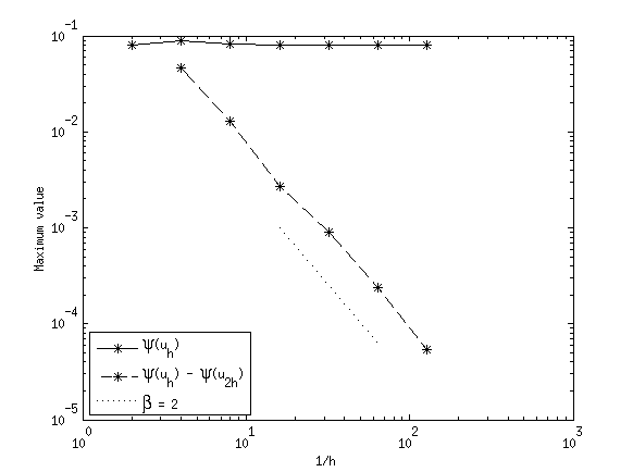
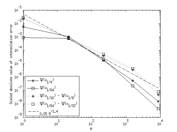
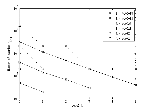
We start by confirming, in Figure 1, the assumptions of Theorem 9. The reference values are computed with spatial mesh width and stochastic interpolation level .
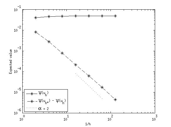
The top-left plot of Figure 1 shows the convergence of the finite element error in the expected value of , and confirms that assumption F1 of Theorem 9 holds with .
The top-right plot of Figure 1 shows the behavior of the function from Theorem 13 for the quantities and . We see that whereas is bounded by a constant independent of and decays quadratically in . This confirms assumption F3 with .
The bottom-left plot of Figure 1 shows the interpolation error in scaled by and the interpolation error in scaled by for several values of . According to assumptions F2 and F3, these plots should all result in a straight line , where . The best fit which has and is added for comparison.
The bottom-right plot of Figure 1 shows the number of samples computed using the formula (10), with and , for several values of . The finest level was determined using the estimates on the finite element error from the top-left plot. Solid lines correspond to numbers rounded up to the nearest integer, as is done in (11), whereas dotted lines correspond to the number of samples rounded up to the next level of the sparse grid.
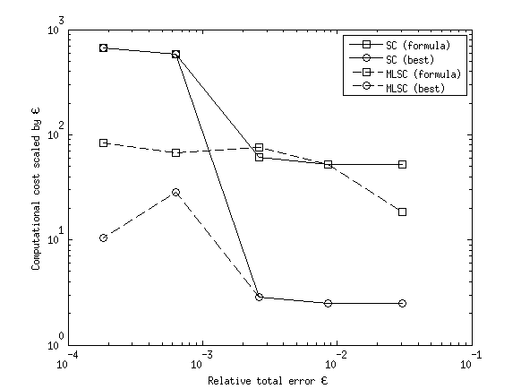
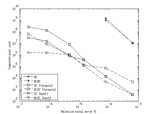
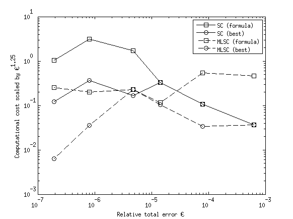
In Figure 2, we study the cost of the standard and multilevel collocation methods to achieve a given total accuracy . In both plots, the data labeled ‘SC’ and ‘MLSC’ denote standard and multilevel stochastic collocation, respectively. For data labeled ‘formula’, the number of samples was determined by the formula (10) with and , rounded up to the next sparse grid level (the dotted lines in the bottom right plot of Figure 1). For data labeled ‘best’, the number of samples was chosen manually so as to achieve a total accuracy for the smallest computational cost. For all methods, we chose .
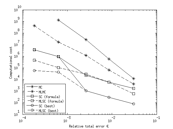
In the left plot of Figure 2, we simply plot the computational cost of the different estimators against . For comparison, we have also added corresponding results for Monte Carlo (MC) and multilevel Monte Carlo (MLMC) estimators. In both the ‘formula’ and the ‘best’ case, the multilevel collocation method outperforms standard SC. Both collocation-based methods outperform both Monte Carlo approaches.
In the right plot in Figure 2, we compare the observed computational cost with that predicted by Theorem 9 for the standard and multilevel collocation methods. In our computations, we observed , , and , which with gives computational costs of and for the multilevel and standard SC method, respectively. We therefore plot the computational cost scaled by . We see that both multilevel methods indeed seem to grow approximately like , with the ‘formula’ case growing slightly faster for large value of and the ‘best’ case growing slightly faster for small values of . The costs for both standard collocation methods grow a lot faster with .
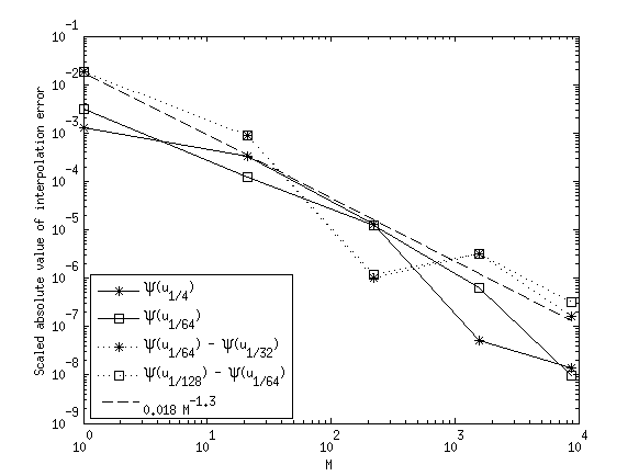
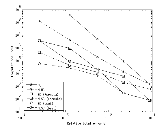
Figure 3 provides results for a different quantity of interest, . The left plot corresponds to the bottom-left plot in Figure 1 and again confirms that the interpolation error in scales with . The right plot corresponds to the left plot of Figure 2, where we plot the computational cost of the different estimators against . We see that all collocation-based methods outperform the Monte Carlo approaches. In both the ‘formula’ and the ‘best’ case, the multilevel collocation method again outperforms standard SC.
Remark 22.
Before considering the second model problem, let us briefly comment on the differences between the ‘best’ and the ‘formula’ multilevel methods. The ‘formula’ multilevel collocation method performs sub-optimally mainly for two reasons. First, it always rounds up the number of samples to the nearest sparse grid level, which may be substantially higher than the number of samples actually required. Secondly, it does not take into account sign changes in the interpolation error, which in practice can lead to significant reductions in the interpolation error of the multilevel method. For both of these reasons, the interpolation error is often a lot smaller than the required , leading to sub-optimal performance. This issue is partly addressed in Section 6.3, where we consider not always rounding up, but rounding the number of samples either up or down to the nearest sparse grid level.
6.2
We now repeat the numerical tests done in the previous section for the case and . For the quantity of interest, we choose the expected value of the solution evaluated at . The reference values are computed using the mesh width and interpolation level .
We again start by confirming, in Figure 4, the assumptions of Theorem 9. The four plots of that figure convey the same information as do the corresponding plots in Figure 1 and again confirm assumptions F1, F2, and F3 of that theorem with and and, in the bottom-right plot, the best line fit with and .
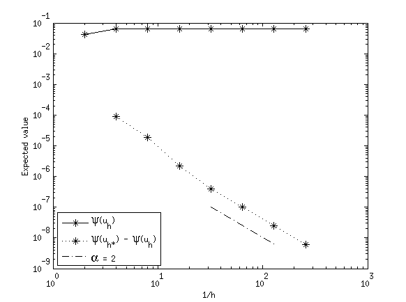
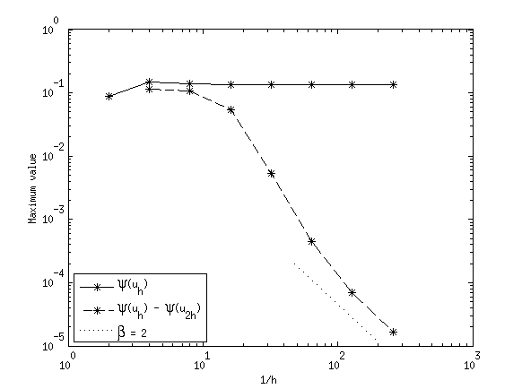
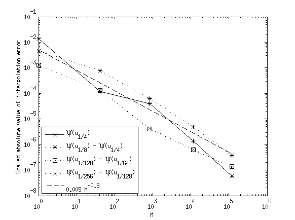
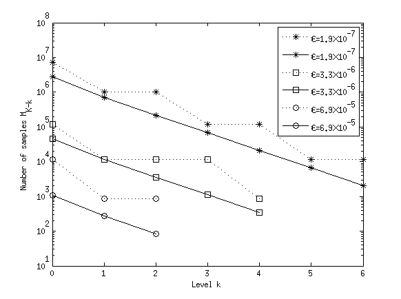
Figure 5 conveys the same information and uses the same labeling as does Figure 2. Again, for both the ‘formula’ and ‘best’ cases, the multilevel collocation method eventually outperforms standard SC and both collocation-based methods also outperform the Monte Carlo approaches. Based on the values , , and , Theorem 9 now predicts the computational costs of and for the multilevel and the standard collocation methods, respectively. The right-plot in Figure 5 indicates that the ‘formula’ multilevel collocation method indeed seems to grow like whereas the ‘best’ multilevel method actually seems to grow slower for small values of . This is likely due to the different signs of the interpolation errors in the multilevel estimator. Also, again, the costs for both standard collocation methods grow a lot faster with .
6.3 Practical implementation
In Sections 6.1 and 6.2, the accuracy of the computed estimates was assessed by comparison to a reference solution. Of course, in practice, a fine-grid, high-level reference solution is not available. Therefore, in this section, we describe how to implement the MLSC method without having recourse to a reference solution. We suggest the following practical strategy that is similar to the one proposed in [12].
-
1.
Estimate the constants , , , and .
-
2.
Start with .
-
3.
Calculate the optimal number of samples , according to the formula (10), and round to the nearest sparse grid level.
-
4.
Test for convergence using
-
5.
If not converged, set and return to step 3.
Note that in this procedure, steps 3 and 4 ensure that the interpolation error and the spatial discretization error are each less than the required tolerance , respectively.
The estimation of the constants , , , and in step 1 can be done relatively cheaply from computations done using mesh widths , , and and interpolation levels . For the results provided below, we estimated the convergence rate from the level 1 interpolants of , , and , resulting in . In light of the results in Section 5, we assumed . We then used the first three interpolation levels of and to obtain the estimates and . Note that the value of is the same as in Section 6.2 whereas the value of the constant is slightly larger. This is due to the fact that, for the large values of used to estimate this constant, the function has probably not yet settled into its asymptotic quadratic decay.
As mentioned in Section 6.1, always rounding the number of samples resulting from formula (10) up to the next sparse grid level may lead to a substantial increase in the computational cost and hence a sub-optimal performance of the multilevel method. In practice, one might therefore consider not always rounding up, but instead rounding either up or down. As long as we do not round down more frequently than we round up, or at least not much more often, this approach should still result in an interpolation error below the required tolerance .
Table 3 shows the number of samples resulting from the implementation described in this section for the model problem with and from Section 6.2. For each value of , the first row, denoted by ‘formula’, corresponds to the numbers resulting from formula (10) rounded up to the nearest integer. The second row, denoted ‘up’, are the numbers in the first row rounded up to the next corresponding sparse grid level. For the final row, denoted ‘up/down’, the rounding of the number of samples was done in the following way: First, all numbers were rounded either up or down to the nearest corresponding sparse grid level. If this resulted in more numbers being rounded down than up, we chose the number that was rounded down by the largest amount and then instead rounded this number up. This procedure was continued iteratively. The same was done when more numbers were rounded up than down.
| level | 0 | 1 | 2 | 3 | 4 | |
|---|---|---|---|---|---|---|
| 6.3e-4 | formula | 191 | 48 | 15 | ||
| up | 841 | 841 | 41 | |||
| up/down | 841 | 41 | 41 | |||
| 7.9e-5 | formula | 3002 | 747 | 233 | 73 | |
| up | 11561 | 841 | 841 | 841 | ||
| up/down | 841 | 841 | 841 | 41 | ||
| 1.4e-5 | formula | 27940 | 6949 | 2169 | 677 | 212 |
| up | 120401 | 11561 | 11561 | 841 | 841 | |
| up/down | 11561 | 11561 | 841 | 841 | 841 | |
| 4.7e-6 | formula | 110310 | 27433 | 8562 | 2672 | 834 |
| up | 120401 | 120401 | 11561 | 11561 | 841 | |
| up/down | 120401 | 11561 | 11561 | 11561 | 841 |
To confirm that the adaptive procedure still achieves the required tolerance on the total error, we have, for Table 4, computed the stochastic interpolation and finite element errors (with respect to a reference solution) and the computational cost of the multilevel approximations from Table 3. For comparison, we have added the results for the multilevel method which was manually found to give a total error less than at minimal cost, which was already computed in Section 6.2 assuming a reference solutions was available. Note that for large values of , the adaptive procedure described in this section overestimated the finite element error, leading to a larger number of levels compared to that found in Section 6.2. It is clear from Table 4 that not only does the alternative rounding procedure yield the required bound on the error, it also significantly reduces the computational cost of the multilevel method, bringing it close to what was manually found to be the minimal cost possible.
| Interpolation error | Spatial error | Cost | ||
|---|---|---|---|---|
| 6.3e-4 | up | 6.7e-5 | 3.4e-5 | 8266 |
| up/down | 2.8e-4 | 3.4e-5 | 4902 | |
| best | 8.0e-5 | 2.9e-4 | 369 | |
| 7.9e-5 | up | 2.2e-5 | 6.3e-6 | 85558 |
| up/down | 3.0e-5 | 6.3e-6 | 15650 | |
| best | 2.4e-5 | 3.4e-5 | 4591 | |
| 1.4e-5 | up | 2.7e-6 | 1.6e-6 | 853207 |
| up/down | 8.3e-6 | 1.6e-6 | 158714 | |
| best | 3.9e-6 | 6.3e-6 | 119699 | |
| 4.7e-6 | up | 7.3e-8 | 1.6e-6 | 1519787 |
| up/down | 1.2e-6 | 1.6e-6 | 1038183 | |
| best | 1.2e-6 | 1.6e-6 | 1038183 |
7 Concluding remarks
Computing solutions of stochastic partial differential equations using stochastic collocation methods can become prohibitively expensive as the dimension of the random parameter space increases. Drawing inspiration from recent work in multilevel Monte Carlo methods, this work proposed a multilevel stochastic collocation method, based on a hierarchy of spatial and stochastic approximations. A detailed computational cost analysis showed, in all cases, a sufficient improvement in costs compared to single-level methods. Furthermore, this work provided a framework for the analysis of a multilevel version of any method for SPDEs in which the spatial and stochastic degrees of freedom are decoupled.
The numerical results practically demonstrated this significant decrease in complexity versus single level methods for each of the problems considered. Likewise, the results for the model problem showed multilevel SC to be superior to multilevel MC even up to dimensions.
One of the largest obstacles to the practicality of stochastic collocation methods is the huge growth in the number of points between grid levels. In the multilevel case, this can lead to a large amount of computational inefficiency. Certain simple rounding schemes were proposed to mitigate this effect, and proved to be extremely effective for the problems considered. Similarly, since most of our example problems involved computation of a reference solution for the estimation of the necessary constants, a more practical multilevel stochastic collocation algorithm that dispensed with the need for a reference solution was proposed and tested.
It is clear that for any sampling method for SPDEs, whether Monte Carlo or stochastic collocation, multilevel methods are to be preferred over single-level methods for improved efficiency. Especially in the case of stochastic collocation methods, multilevel approaches enable one to further delay the curse of dimensionality, tempering the explosion of computational effort that results when the stochastic dimension increases. Though Monte Carlo methods are often preferable for problems involving a large stochastic dimension, multilevel approaches greatly improve the effectiveness of stochastic collocation methods versus Monte Carlo methods.
Acknowledgements
The first and the fourth authors are supported by the US Department of Defense Air Force Office of Scientific Research (AFOSR) under grant number FA9550-11-1-0149 and by he US Department of Energy Advance Simulation Computing Research (ASCR) program under grant number DE-SC0010678.
The second and third authors are supported by the US AFOSR under grant number 1854-V521-12 and by the US Department of Energy ASCR under grant number ERKJ259. Also supported by the Laboratory Directed Research and Development (LDRD) Program at the Oak Ridge National Laboratory (ORNL). The ORNL is operated by UT-Battelle, LLC, for the US Department of Energy under Contract DE-AC05-00OR22725.
References
- [1] Ivo Babuška, Fabio Nobile, and Raul Tempone, A Stochastic Collocation Method for Elliptic Partial Differential Equations with Random Input Data, SIAM Journal on Numerical Analysis, 45 (2007), pp. 1005–1034.
- [2] Andrea Barth, Christoph Schwab, and Nathaniel Zollinger, Multi-level Monte Carlo Finite Element method for elliptic PDEs with stochastic coefficients, Numerische Mathematik, 119 (2011), pp. 123–161.
- [3] S.C. Brenner and L.R. Scott, The Mathematical Theory of Finite Element Methods, vol. 15 of Texts in Applied Mathematics, Springer, third ed., 2008.
- [4] J. Charrier, Strong and weak error estimates for the solutions of elliptic partial differential equations with random coefficients, SIAM J. Numer. Anal, 50 (2012), pp. 216–246.
- [5] J Charrier, R Scheichl, and A L Teckentrup, Finite element error analysis of elliptic PDEs with random coefficients and its application to multilevel Monte Carlo methods, SIAM Journal on Numerical Analysis, 51 (2013), pp. 322–352.
- [6] P. G. Ciarlet, The Finite Element Method for Elliptic Problems, North–Holland, 1978.
- [7] KA Cliffe, MB Giles, Robert Scheichl, and Aretha L Teckentrup, Multilevel monte carlo methods and applications to elliptic pdes with random coefficients, Computing and Visualization in Science, 14 (2011), pp. 3–15.
- [8] S. Dereich and F. Heidenreich, A multilevel Monte Carlo algorithm for Lévy-driven stochastic differential equations, Stochastic Process. Appl., 121 (2011), pp. 1565–1587.
- [9] P. Frauenfelder, Ch. Schwab, and R.A. Todor, Finite elements for elliptic problems with stochastic coefficients, Comput. Methods Appl. Mech. Engrg., 194 (2005), pp. 205–228.
- [10] R. G. Ghanem and P. D. Spanos, Stochastic finite elements: a spectral approach, Springer-Verlag, New York, 1991.
- [11] M.B. Giles and C. Reisinger, Stochastic finite differences and multilevel Monte Carlo for a class of SPDEs in finance, SIFIN, 1 (2012), pp. 575–592.
- [12] Michael B Giles, Multilevel monte carlo path simulation, Operations Research, 56 (2008), pp. 607–617.
- [13] C.J. Gittelson, J. Könnö, Ch. Schwab, and R. Stenberg, The multilevel Monte Carlo finite element method for a stochastic Brinkman problem, Numer. Math., (published online March 2013).
- [14] Helmut Harbrecht, Michael Peters, and Markus Siebenmorgen, On multilevel quadrature for elliptic stochastic partial differential equations, in Sparse Grids and Applications, Springer, 2013, pp. 161–179.
- [15] Stefan Heinrich, Multilevel monte carlo methods, in Large-scale scientific computing, Springer, 2001, pp. 58–67.
- [16] H. Hoel, E. von Schwerin, A. Szepessy, and R. Tempone, Adaptive multilevel Monte Carlo simulation, in Numerical Analysis of Multiscale Computations, B. Engquist, O. Runborg, and Y.-H. R. Tsai, eds., vol. 82 of Lecture Notes in Comput. Sci., Springer, 2012, pp. 217–234.
- [17] F. Nobile, R. Tempone, and C. Webster, A sparse grid stochastic collocation method for partial differential equations with random input data, SIAM J. Numer. Anal., 46 (2008), pp. 2309–2345.
- [18] F. Nobile, R. Tempone, and C. G. Webster, An anisotropic sparse grid stochastic collocation method for partial differential equations with random input data, SIAM J. Numer. Anal., 46 (2008), pp. 2411–2442.
- [19] A. L. Teckentrup, R. Scheichl, M. B. Giles, and E. Ullmann, Further analysis of multilevel Monte Carlo methods for elliptic PDEs with random coefficients, Numer. Math., (published online March 2013).