Contrasting the wide Feshbach resonances in ⁶Li and ⁷Li

Abstract

We compare and contrast the wide Feshbach resonances and the corresponding weakly bound states in the lowest scattering channels of ultracold ⁶Li and ⁷Li. We use high-precision measurements of binding energies and scattering properties to determine interaction potentials that incorporate non-Born-Oppenheimer terms to account for the failure of mass scaling between ⁶Li and ⁷Li. Correction terms are needed for both the singlet and the triplet potential curves. The universal formula relating binding energy to scattering length is not accurate for either system. The ⁶Li resonance is open-channel-dominated and the van der Waals formula of Gao [J. Phys. B 37, 4273 (2004)] gives accurate results for the binding energies across much of the resonance width. The ⁷Li resonance, by contrast, is weakly closed-channel-dominated and a coupled-channels treatment of the binding energies is required. Plotting the binding energies in universal van der Waals form helps illustrate subtle differences between the experimental results and different theoretical forms near the resonance pole.

I Introduction

The magnetically tunable threshold scattering resonances of two atoms provide a powerful tool for investigating many-body and few-body phenomena in ultracold quantum gases Chin et al. (2010). Here we compare and contrast the wide resonances of the species ⁶Li and ⁷Li using accurate quantum scattering calculations interpreted within the framework of universal van der Waals quantum defect theory. These Li resonances, which are quite different in character despite a superficial similarity in magnetic-field width Chin et al. (2010), have been used in numerous experimental studies involving the ⁶Li fermion Cubizolles et al. (2003); Jochim et al. (2003); Strecker et al. (2003); Bourdel et al. (2004); Zwierlein et al. (2004); Bartenstein et al. (2005); Schunck et al. (2005); Partridge et al. (2005); Zwierlein et al. (2005, 2006); Partridge et al. (2006); Zürn et al. (2013) or ⁷Li boson Abraham et al. (1997); Bradley et al. (1997); Strecker et al. (2002); Pollack et al. (2009); Gross et al. (2009, 2010, 2011); Rem et al. (2013); Dyke et al. (2013). They serve as a prototype of the variations encountered among the many different resonances and species of interest for ultracold physics. Using the universal properties of the van der Waals potential gives a powerful way to characterize the variation in resonance properties in terms of dimensionless variables.

The fundamental quantity for studies of the interactions of ultracold atoms at very small collision energy $E$ is the $s$-wave scattering length, which can be tuned approximately according to the resonant formula Moerdijk et al. (1995); Chin et al. (2010)

$$a(B)=a_{\mathrm{bg}}\left(1-\frac{\Delta}{B-B_{0}}\right)\,,$$ (1)

where $a_{\mathrm{bg}}$ is a near-constant “background” scattering length far from the resonance pole at magnetic field $B=B_{0}$ and $\Delta$ is the resonance width. The resonance is due to the variation with magnetic field of the energy of a “closed-channel” bound state with a magnetic moment $\mu_{\mathrm{mol}}$ that is different from the combined magnetic moment $\mu_{\mathrm{atoms}}$ of the two separated atoms that define the open entrance channel. The mixing of the “bare” or uncoupled open and closed channels results in a coupled-channels bound state with an energy $E_{\mathrm{b}}$ that is universally related to the scattering length when the latter is sufficiently large Chin et al. (2010),

$$E_{\mathrm{b}}(B)\approx-\frac{\hbar^{2}}{2\mu a(B)^{2}}\,,$$ (2)

where $\mu$ is the reduced mass of the pair of atoms. While this equation is widely used, it is actually not quantitatively very accurate until the scattering length become extraordinarily large, and departures from it show up readily in experimental measurements of binding energies. In fact, the binding energy of a Feshbach molecule comprised of two ⁶Li atoms in different spin states has been measured so accurately Zürn et al. (2013) that the actual binding energy of the resonant state deviates from the universal value in Eq. (2) by 200 times the measurement uncertainty, even when the scattering length is on the order of 2000 $a_{0}$, where $a_{0}$ is the Bohr radius. We will use accurate coupled-channels calculations to investigate the relationship between $E_{\mathrm{b}}(B)$ and $a(B)$ for resonances for both ⁶Li atoms and ⁷Li atoms, and compare these to the predictions of simple single-channel formulas that correct Eq. (2) in the case of a van der Waals potential Gribakin and Flambaum (1993); Gao (2004); Chin et al. (2010). The two species show quite different departures from the universal formula because of their very different resonance character.

The long-range potential between two S-state neutral atoms has the van der Waals form $-C_{6}/R^{6}$, where $R$ is the interatomic distance. The strength of the van der Waals potential sets a characteristic length and energy associated with low-energy collisions Gribakin and Flambaum (1993); Chin et al. (2010),

$$\bar{a}=\frac{2\pi}{\Gamma(\frac{1}{4})^{2}}\left(\frac{2\mu C_{6}}{\hbar^{2}}\right)^{\frac{1}{4}};\qquad\bar{E}=\frac{\hbar^{2}}{2\mu\bar{a}^{2}}.$$ (3)

Using $C_{6}=$ 1393.39 E${}_{\mathrm{h}}a_{0}^{6}$ Yan et al. (1996), where $E_{\rm h}$ is the Hartree energy, and the respective values of $\bar{a}$ and $\bar{E}/h$ are 29.884 $a_{0}$ and 671.93 MHz for two ⁶Li atoms and 31.056 $a_{0}$ and 533.41 MHz for two ⁷Li atoms.

Ultracold $s$-wave collisions occur in the domain of collision energy $E\ll\bar{E}$ or, correspondingly, of de Broglie wavelength $2\pi/k\gg\bar{a}$, where $\hbar k$ is the relative collision momentum. Furthermore, the “pole strength” of the resonant pole in $a(B)$ in Eq. (1) is characterized by a dimensionless parameter $s_{\mathrm{res}}=(a_{\mathrm{bg}}/\bar{a})(\delta\mu\Delta/\bar{E})$, where $\delta\mu=\mu_{\mathrm{atoms}}-\mu_{\mathrm{mol}}$. Chin et al. Chin et al. (2010) distinguish two distinct types of resonance. Those with $s_{\mathrm{res}}\gg 1$ are “open-channel-dominated” and have a bound state that takes on the character of the open entrance channel over a tuning range spanning much of the width of the resonance. By contrast, “closed-channel-dominated” resonances with $s_{\mathrm{res}}\ll 1$ have bound states that take on the character of the closed channel except when $B$ is tuned very close to the resonance pole. The ⁶Li and ⁷Li resonances that we study have respective $s_{\mathrm{res}}$ parameters of 59 Chin et al. (2010) and 0.49 Jachymski and Julienne (2013), and thus show very different relationships between $E_{\mathrm{b}}(B)$ and $a(B)$, in spite of the fact that they have widths $\Delta$ of similar magnitude.

For heavy diatomic molecules, the differences between the binding energies for different isotopes can be well accounted for by retaining the same potential curves and simply changing the masses used in the calculation  Seto et al. (2000); Docenko et al. (2007); Falke et al. (2008); Kitagawa et al. (2008); Strauss et al. (2010); Brue and Hutson (2013); Borkowski et al. (2013). However, it is known that mass corrections due to the breakdown of the Born-Oppenheimer approximation are important for light species like H₂ Kołos and Wolniewicz (1964, 1965), and also have significant effects in LiK Tiemann et al. (2009) and LiRb Ivanova et al. (2011). For the case of Li₂, Le Roy and coworkers have analyzed extensive electronic spectra and have shown that mass corrections are essential for both the singlet Le Roy et al. (2009) and triplet Dattani and Le Roy (2011) states. In order to reproduce the resonance positions, we also find that we have to use slightly different singlet and triplet potentials for the two isotopes. The mass corrections correspond to an isotopic shift of about 4 G in the position of the ⁷Li resonance from its mass-scaled position.

This paper will describe the basic molecular physics of the near-threshold states of the Li₂ molecule and our fitting of the potentials to the combined experimental results for ⁶Li₂ and ⁷Li₂. Our potentials reproduce the measured threshold two-body results for both isotopes. We will then compare the binding energies calculated from our coupled-channels models, using a universal van der Waals form to demonstrate the near-threshold relationships between scattering length and binding energy and to test the approximate formulas that have been developed to treat this relationship. Both isotopes exhibit clear deviation from the universal predictions of Eq. (2), even in regions of magnetic tuning where the scattering length is large compared to $\bar{a}$. However, the behavior depends upon the value of the $s_{\mathrm{res}}$ parameter. We will show that the formula of Gao Gao (2004) for the bound states in a single van der Waals potential provides a good approximation for the strong resonance in ⁶Li₂ but fails to represent the binding energies for the much weaker resonance in ⁷Li₂.

II Overview of ⁶Li and ⁷Li

Figure 1 shows the hyperfine/Zeeman atomic structure of the ²S_1/2 ground state of the ⁶Li and ⁷Li atoms. The electron spin $s=\frac{1}{2}$ couples to the nuclear spin $i$ to give a resultant atomic spin $f$ with projection $m_{f}$. When $B$ is non-zero, the states of different $f$ mix, but the projection $m_{f}$ remains a good quantum number. We designate the atomic states in order of increasing energy by the labels 1, 2, $\ldots$ for each species. A collision of two atoms is characterized by their relative angular momentum given by the partial-wave quantum number $L$. We are interested in the lowest-energy $L=0$ ($s$-wave) spin channels of ⁶Li₂ and ⁷Li₂, for which the Feshbach resonances have been identified and characterized. These are the (1,2) channel of ⁶Li₂ Schunck et al. (2005); Bartenstein et al. (2005); Zürn et al. (2013) with $M_{F}=m_{f,{\rm a}}+m_{f,{\rm b}}=0$ and the (1,1) Pollack et al. (2009); Gross et al. (2010, 2011); Rem et al. (2013); Dyke et al. (2013) and (2,2) Gross et al. (2009, 2011) channels of ⁷Li₂ with $M_{F}=$ 2 and 0 respectively. Here we label the channels by the states $(i,j)$ of the two separated atoms.

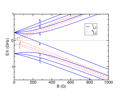
Figure 1: (Color online) Energy levels of the ²S_1/2 ground state of the ⁶Li and ⁷Li atoms, showing the different hyperfine structure of the two isotopes, which at zero field have upper and lower total angular momentum quantum numbers $f$=$\frac{1}{2}$ and $\frac{3}{2}$ for ⁶Li and $f=$ 1 and 2 for ⁷Li. The energy zero is the energetic center of gravity of the hyperfine multiplet. The numbers indicate the state labels for all the states of ⁷Li and the lowest two states of ⁶Li. The lowest and highest-energy states at finite $B$ have $m_{f}$=$+\frac{1}{2}$ and $+\frac{3}{2}$ for ⁶Li and $m_{f}$=+1 and +2 for ⁷Li.

Figure 2 shows the adiabatic potential energy curves for the lowest singlet and triplet states of the Li₂ molecule, ${}^{1}\Sigma_{g}^{+}$ and ${}^{3}\Sigma_{u}^{+}$. The inset shows the asymptotic hyperfine structure for the five spin channels of ⁷Li₂ that have projection $M_{F}=2$, which are (1,1), (1,7), (2,8), (6,8) and (7,7). For a light species like Li, where the spacing between vibrational levels is much larger than the atomic hyperfine splitting, the molecular bound states, even near threshold, are primarily of either ${}^{1}\Sigma_{g}^{+}$ or ${}^{3}\Sigma_{u}^{+}$ character. The inset of Fig. 2 indicates the energy $-2.668$ GHz $\times\ h$ of the last zero-field $s$-wave bound state of the ⁷Li₂ molecule; this is the $v=41$ vibrational level of the ${}^{1}\Sigma_{g}^{+}$ potential, with total nuclear spin $I=2$ and projection $M_{I}=2$. The next $s$-wave bound states down from threshold are the hyperfine components of a ${}^{3}\Sigma_{u}^{+}$ level near $-12$ GHz. A similar figure for ⁶Li in Ref. Chin et al. (2010) shows the long-range hyperfine channels for the $M_{F}=0$ states of ⁶Li₂; in this case the highest zero-field level is the $v=38$ vibrational level of the ${}^{1}\Sigma_{g}^{+}$ state, which has two nuclear spin components $I=0$, $M_{I}=0$ and $I=2$, $M_{I}=0$ that lie respectively at $-1.625$ GHz and $-1.612$ GHz. The next ⁶Li₂ levels down are components of the ${}^{3}\Sigma_{u}^{+}$ state near $-24$ GHz.

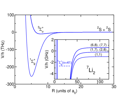
Figure 2: (Color online) Born-Oppenheimer potential energy curves of the Li₂ molecule correlating with two ground-state atoms. The inset shows the adiabatic potential curves of the 5-channel potential matrix at $B=0$ for the states with partial wave $L=0$ ($s$-wave) and total spin projection $M_{\mathrm{tot}}=2$, using the notation of Fig. 1 to label the channels. The inset also shows the location of the last zero-field $s$-wave level of the ⁷Li₂ molecule.

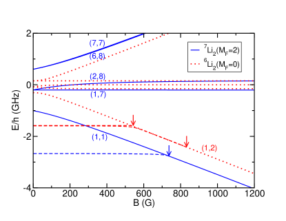
Figure 3: (Color online) Energies of the separated-atom channels for $s$-wave scattering with total spin projection $M_{F}=2$ for ⁷Li₂ (solid lines) and $M_{F}=0$ for ⁶Li₂ (dotted lines). The dashed lines show the energy of the last molecular bound state in each case. The arrows show the pole positions $B_{0}$ of the Feshbach resonances in the lowest-energy $s$-wave channel of each species.

Figure 3 shows the separated-atom energies for the respective $M_{F}=0$ and $M_{F}=2$ states of ⁶Li₂ and ⁷Li₂. The upper dashed line for ⁶Li₂ shows the $v=38$, $I=2$, $M_{I}=0$ ${}^{1}\Sigma_{g}^{+}$ level that is very weakly coupled to the entrance-channel continuum. It crosses threshold near 543.26 G to make a very narrow closed-channel-dominated resonance Strecker et al. (2003); Schunck et al. (2005); Chin et al. (2010); Hazlett et al. (2012). The lower dashed line shows the bound state that makes the very broad open-channel-dominated resonance near 832 G Bartenstein et al. (2005); Zürn et al. (2013). For fields below approximately 540 G, this bound state has the character of the $v=38$, $I=0$, $M_{I}=0$ ${}^{1}\Sigma_{g}^{+}$ level, but it switches at higher $B$ to become the last ($v=10$) level of the ${}^{3}\Sigma_{u}^{+}$ state, with the spin character of the $(1,2)$ channel. Above about 600 G, it is a halo state of open-channel character and produces a scattering length that is large compared to the van der Waals length for a field range spanning nearly 200 G below resonance, or approximately 70% of the resonance width $\Delta\approx$ 300 G Chin et al. (2010). While the $v=41$, $I=2$, $M_{I}=2$ ${}^{1}\Sigma_{g}^{+}$ level of ⁷Li shown in Fig. 3 also produces a resonance with a large width $\Delta\approx$ 170 G Gross et al. (2011); Dyke et al. (2013), in this case the bound state takes on the character of an open-channel halo molecule over only approximately 1% of the resonance width, very close to the resonance pole. We will demonstrate that the very different character of the ⁶Li and ⁷Li resonances shows up clearly in precise measurements of binding energies.

The scattering lengths for ⁶Li and ⁷Li are shown as a function of magnetic field in Fig. 4. Despite the similarity in magnetic-field widths $\Delta$, it may be seen that they have visually quite different pole strengths corresponding to their different $s_{\rm res}$ values. The magnetic-field width $\Delta$ for ⁷Li is in a sense anomalously large because the resonance has a very small background scattering length.

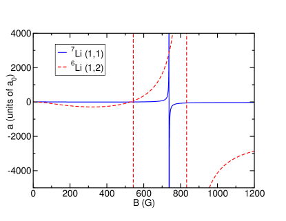
Figure 4: (Color online) Scattering length $a$ as a function of magnetic field $B$ for the (1,2) channel of ⁶Li and the (1,1) channel of ⁷Li, showing the difference in pole strength for the two systems despite a superficial similarity in magnetic-field width $\Delta$. The feature near 543 G in ⁶Li is an additional narrow resonance.

III Theoretical model

The Hamiltonian for the interaction of two alkali-metal atoms in their ground ${}^{2}S$ states may be written

$$\frac{\hbar^{2}}{2\mu}\left[-R^{-1}\frac{d^{2}}{dR^{2}}R+\frac{\hat{L}^{2}}{R^{2}}\right]+\hat{h}_{1}+\hat{h}_{2}+\hat{V}(R),$$ (4)

where $\hat{L}^{2}$ is the operator for the end-over-end angular momentum of the two atoms about one another, $\hat{h}_{1}$ and $\hat{h}_{2}$ are the monomer Hamiltonians, including hyperfine couplings and Zeeman terms, and $\hat{V}(R)$ is the interaction operator.

In the present work we solve the bound-state and scattering problems by coupled-channels calculations using the MOLSCAT Hutson and Green (1994) and BOUND Hutson (1993) packages, as modified to handle magnetic fields González-Martínez and Hutson (2007). Both scattering and bound-state calculations use propagation methods and do not rely on basis sets in the interatomic distance coordinate $R$. The methodology is exactly the same as described for Cs in Section IV of Ref. Berninger et al. (2013), so will not be repeated here. The basis sets included all functions for $L=0$ and $L=2$ with the required $M_{\rm tot}=M_{F}+M_{L}$. The energy-dependent $s$-wave scattering length $a(k)$ is obtained from the diagonal S-matrix element in the incoming channel,

$$a(k)=\frac{1}{ik}\left(\frac{1-S_{00}}{1+S_{00}}\right),$$ (5)

where $k^{2}=2\mu E/\hbar^{2}$ and $E$ is the kinetic energy Hutson (2007).

The interaction operator $\hat{V}(R)$ may be written

$${\hat{V}}(R)=\hat{V}^{\rm c}(R)+\hat{V}^{\rm d}(R).$$ (6)

Here $\hat{V}^{\rm c}(R)=V_{0}(R)\hat{\cal{P}}^{(0)}+V_{1}(R)\hat{\cal{P}}^{(1)}$ is an isotropic potential operator that depends on the electronic potential energy curves $V_{0}(R)$ and $V_{1}(R)$ for the lowest singlet and triplet states of Li₂, as shown in Figure 2. The singlet and triplet projectors $\hat{\cal{P}}^{(0)}$ and $\hat{\cal{P}}^{(1)}$ project onto subspaces with total electron spin quantum numbers 0 and 1 respectively. The term $\hat{V}^{\rm d}(R)$ accounts for the dipolar interaction between the magnetic moments of the two atoms, and for Li is represented simply as

$$\hat{V}^{\rm d}(R)=\frac{E_{\rm h}\alpha^{2}}{(R/a_{0})^{3}}\left[\hat{s}_{1}\cdot\hat{s}_{2}-3(\hat{s}_{1}\cdot\vec{e}_{R})(\hat{s}_{2}\cdot\vec{e}_{R})\right]\,,$$ (7)

where $\vec{e}_{R}$ is a unit vector along the internuclear axis and $\alpha\approx 1/137$ is the fine-structure constant.

At long range, the electronic potentials are

$$V_{S}^{\rm LR}(R)= - C_{6}/R^{6}-C_{8}/R^{8}-C_{10}/R^{10}$$ (8)

$$\pm V_{\rm ex}(R),$$

where $S=0$ and 1 for singlet and triplet, respectively. The dispersion coefficients $C_{n}$ are common to both potentials and are taken from Yan et al. Yan et al. (1996). The exchange contribution is Smirnov and Chibisov (1965)

$$V_{\rm ex}(R)=A(R/a_{0})^{\gamma}\exp(-\beta R/a_{0}),$$ (9)

with parameters $\beta=1.25902\ a_{0}^{-1}$ and $\gamma=4.55988$ Côté et al. (1994). The prefactor $A$ is chosen to match the difference between the singlet and triplet potentials at $R=15.5\ a_{0}$. The exchange term makes an attractive contribution for the singlet and a repulsive contribution for the triplet.

The detailed shapes of the short-range singlet and triplet potentials are relatively unimportant for the ultracold scattering properties and near-threshold binding energies considered here, although it is crucial to be able to vary the volume of the potential wells to allow adjustment of the singlet and triplet scattering lengths. In the present work we retained the functional forms used by O’Hara et al. O’Hara et al. (2002) and Zürn et al. Zürn et al. (2013), which are based on the short-range singlet potential of Coté et al. Côté et al. (1994) and the short-range triplet potential of Linton et al. Linton et al. (1999). We used the methodology of Ref. Côté et al. (1994) to connect the short-range and long-range potentials.

The flexibility needed to adjust the singlet and triplet scattering lengths is provided by simply adding a quadratic shift to each of the singlet and triplet potentials inside its minimum,

$$V_{S}^{\rm shift}(R)=S_{S}(R-R_{eS})^{2}\hbox{\qquad for\qquad}R<R_{eS},$$ (10)

with $R_{e0}=2.673247$ Å and $R_{e1}=4.173$ Å.

IV Fitting interaction potentials

We have carried out simultaneous fits to experimental results for the scattering properties and near-threshold bound states of both ⁶Li and ⁷Li. For ⁶Li the experimental data set was exactly the same as for the fitting described in ref. Zürn et al. (2013), and was made up of highly precise bound-state energies $E_{\rm b}$, expressed as frequencies $\nu_{\rm b}=|E_{\rm b}|/h$, for the (1,2) channel at fields between 720 and 812 G Zürn et al. (2013), together with transition frequencies between states in the (1,2) and (1,3) channels at fields between 660 and 690 G Bartenstein et al. (2005) and a precise measurement of the position of the zero-crossing in the scattering length for the (1,2) channel Du et al. (2008). For ⁷Li we fitted to a subset of the bound-state energies for the (1,1) channel measured by Dyke et al. Dyke et al. (2013) at fields between 725 and 737 G, together with measurements of a zero-crossing in the (1,1) channel Pollack et al. (2009) and two poles in the (2,2) channel Gross et al. (2011). We carried out direct least-squares fitting to the results of coupled-channels calculations, using the I-NoLLS package Law and Hutson (1997) (Interactive Non-Linear Least-Squares), which gives the user interactive control over step lengths and assignments as the fit proceeds.

As described above, it is not adequate to use the same interaction potentials for ⁶Li and ⁷Li and to rely on mass-scaling (and changes in hyperfine parameters) to reproduce the results for both isotopes. We have therefore chosen to introduce different short-range shift parameters $S_{0}$ and $S_{1}$ for the two isotopes, with the difference between them as explicit fitting parameters. We define $S_{S}^{(7)}=S_{S}^{(6)}+\Delta S_{S}$ and fit to the 4 parameters $S_{0}^{(6)}$, $\Delta S_{0}$, $S_{1}^{(6)}$ and $\Delta S_{1}$. In principle we could also fit to additional parameters such as $C_{6}$, $C_{8}$, etc., as was done for Cs Berninger et al. (2013), but this was not found to be necessary to reproduce the threshold results for Li.

6Li	Present fit		Experiment
$\nu_{\rm b,12}-\nu_{\rm b,13}+\nu_{\rm ff}$	83 665.9(8)		83 664.5(10)		Bartenstein et al. (2005)
at 661.436 G
$\nu_{\rm b,12}-\nu_{\rm b,13}+\nu_{\rm ff}$	83 297.3(5)		83 296.6(10)		Bartenstein et al. (2005)
at 676.090 G
$\nu_{\rm b,12}$ at 720.965 G	127	.115(58)	127	.115(31)	Zürn et al. (2013)
$\nu_{\rm b,12}$ at 781.057 G	14	.103(37)	14	.157(24)	Zürn et al. (2013)
$\nu_{\rm b,12}$ at 801.115 G	4	.342(24)	4	.341(50)	Zürn et al. (2013)
$\nu_{\rm b,12}$ at 811.139 G	1	.828(16)	1	.803(25)	Zürn et al. (2013)
Zero in $a_{12}$	527	.32(8)	527	.5(2)	Du et al. (2008)
Narrow pole in $a_{12}$	543	.41(12)	543	.286(3)	Hazlett et al. (2012)
$a_{\rm s}$	45	.154(2)
$a_{\rm t}$	$-$2113	(2)

7Li	Present fit		Experiment
Pole in $a_{11}$	737	.69(2)
Zero in $a_{11}$	543	.64(19)	543.6(1)		Pollack et al. (2009)
Pole in $a_{22}$	845	.31(4)	844.9(8)		Gross et al. (2011)
Pole in $a_{22}$	893	.78(4)	893.7(4)		Gross et al. (2011)
$\nu_{\rm b,11}$ at 736.8 G	34	.3(1.0)	40	(3)	Dyke et al. (2013)
$\nu_{\rm b,11}$ at 736.5 G	61	.4(1.3)	62	(2)	Dyke et al. (2013)
$\nu_{\rm b,11}$ at 735.5 G	209	.2(2.3)	212	(2)	Dyke et al. (2013)
$\nu_{\rm b,11}$ at 734.3 G	474	.6(3.5)	469	(3)	Dyke et al. (2013)
$\nu_{\rm b,11}$ at 733.5 G	772	(5)	775	(9)	Dyke et al. (2013)
$\nu_{\rm b,11}$ at 732.1 G	1378	(7)	1375	(10)	Dyke et al. (2013)
$\nu_{\rm b,11}$ at 728.0 G	4114	(14)	4019	(90)	Dyke et al. (2013)
$a_{\rm s}$	34	.331(2)
$a_{\rm t}$	$-$26	.92(7)

Table 1: Quality of fit between coupled-channels calculations on the best-fit 4-parameter Li potential and the experiments, together with key derived quantities calculated using the potential. All frequencies are given in kHz, all lengths in $a_{0}$ and all magnetic fields in G. The quantities in parentheses are statistical 95% confidence limits in the final digits for the fit results and quoted uncertainties for the experiments. The quantity $\nu_{\rm ff}$ is the frequency of the transition between thresholds 2 and 3 for free ⁶Li atoms at the magnetic field concerned.

The set of experimental results used for fitting is listed in Table 1. The quantity optimized in the least-squares fits was the sum of squares of residuals ((obs$-$calc)/uncertainty), with the uncertainties listed in Table 1. We carried out both 3-parameter and 4-parameter fits, either including or excluding the $\Delta S_{1}$ parameter that describes the deviation from mass-scaling for the weakly bound triplet potential. We found that 3-parameter fits were capable of reproducing most of the experimental results, but gave a zero-crossing about 1 G in error for the scattering length in the (1,1) channel for ⁷Li. The 4-parameter fit, by contrast, was able to reproduce this along with all the other data. We thus consider the 4-parameter fit preferable, and give the results based on it in Table 1. The optimized parameter values are given in Table 2, together with their 95% confidence limits Le Roy (1998). The optimized potential for ⁶Li is identical to that of Ref. Zürn et al. (2013), because the data set is identical for this isotope, but the parameter correlations and hence the 95% confidence limits are different in the 4-parameter space used in the present work. It may be seen that the 95% confidence limits for the $\Delta S_{0}$ parameter is less than 2.5% of its value, and even that for the $\Delta S_{1}$ parameters is less than 25% of its value.

Table 2: Parameters of the fitted potential, together with statistical confidence limits and sensitivities that indicate the precision needed to reproduce the calculated quantities.

	fitted value	confidence	sensitivity
		limit (95%)
$S_{0}^{(6)}$ ($\mu E_{\rm h}\,a_{0}^{-2}$)	$-11.8959$	$0.0383$	$0.0003$
$\Delta S_{0}$ ($\mu E_{\rm h}\,a_{0}^{-2}$)	$3.0429$	$0.0714$	$0.0006$
$S_{1}^{(6)}$ ($\mu E_{\rm h}\,a_{0}^{-2}$)	$0.51031$	$0.00203$	$0.00002$
$\Delta S_{1}$ ($\mu E_{\rm h}\,a_{0}^{-2}$)	$0.69955$	$0.15149$	$0.00142$

It should be emphasized that the 95% confidence limits are statistical uncertainties within the particular parameter set. They do not include any errors due to the choice of the potential functions. Such model errors are far harder to estimate, except by performing a large number of fits with different potential models, which is not possible in the present case.

In a correlated fit, the statistical uncertainty in a fitted parameter depends on the degree of correlation. However, to reproduce the results from a set of parameters, it is often necessary to specify many more digits than implied by the uncertainty. A guide to the number of digits required is given by the parameter sensitivity Le Roy (1998), which essentially measures how fast the observables change when one parameter is varied with all others held fixed. This quantity is included in Table 2.

The singlet and triplet scattering lengths and the pole positions of the $s$-wave resonances are not directly observed quantities. Nevertheless, their values may be extracted from the final potential. In addition, the statistical uncertainties in any quantity obtained from the fitted potentials may be obtained as described in Ref. Le Roy, 1998. The values and 95% confidence limits obtained in this way, for both the derived parameters such as scattering lengths and the experimental observables themselves, are given in Table 1. It may be noted that the statistical uncertainties in the calculated properties are independent of the experimental uncertainties, and in some cases are smaller.

V Discussion of Results

V.1 Born-Oppenheimer corrections

For a single potential curve with long-range form $-C_{6}R^{-6}$, the scattering length is given semiclassically by Gribakin and Flambaum (1993)

$$a=\bar{a}\left[1-\tan\left(\Phi-\frac{\pi}{8}\right)\right],$$ (11)

where $\Phi$ is a phase integral evaluated at the threshold energy,

$$\Phi=\int_{R_{0}}^{\infty}\left(\frac{-2\mu V(R)}{\hbar^{2}}\right)^{\frac{1}{2}}\,dR$$ (12)

and $R_{0}$ is the inner turning point at this energy. A value of $a$ thus directly implies the fractional part of $\Phi/\pi$. In the Born-Oppenheimer approximation, $V(R)$ is independent of reduced mass, so that the values of $\Phi/\pi$ for different isotopologues are related by simple mass scaling. For alkali metals heavier than Li, such mass scaling is very accurate Seto et al. (2000); Docenko et al. (2007); Falke et al. (2008); Simoni et al. (2008); Cho et al. (2013); Blackley et al. (2013). For Li, however, significant corrections are needed, as shown in Section IV. Eq. (11) may be used to convert the singlet and triplet scattering lengths in Table 1 into the corresponding fractional parts of $\Phi/\pi$. Together with the reduced mass ratio $\mu^{(7)}/\mu^{(6)}=1.1166394$, these are sufficient to determine unambiguously the integer part of $\Phi/\pi$, which for ⁶Li is 38 for the singlet state and 10 for the triplet state. The resulting values for $\Phi/\pi$ for both isotopes are given in Table 3. Comparison of these values obtained directly from the scattering lengths for ⁷Li with those obtained by mass-scaling the ⁶Li results shows that the non-Born-Oppenheimer terms contribute an additional $-9.4\times 10^{-4}$ to $\Phi/\pi$ for singlet ⁷Li and $-1.7\times 10^{-3}$ for triplet ⁷Li. The deviations from mass-scaling in the scattering lengths thus do not by themselves contain any information on the $R$-dependence of the non-Born-Oppenheimer terms, but do provide a strong constraint on their overall magnitude, which could be included in spectroscopic fits such as those of refs. Le Roy et al. (2009) and Dattani and Le Roy (2011).

Table 3: Phase integrals obtained from the fitted singlet and triplet scattering lengths.

	6Li	mass-scaled	7Li
		6Li to 7Li
$\Phi_{\rm s}/\pi$	38.97463	42.09250	42.09156
$\Phi_{\rm t}/\pi$	10.62056	11.47018	11.46846

V.2 Relationship of binding energy to scattering length

Figure 5 shows the calculated binding energy as a function of $B$ for the (1,1) channel of ⁷Li, illustrating the good agreement with the results of Dyke et al. Dyke et al. (2013). Our calculation also agrees well with the results of Navon et al. Navon et al. (2011), although we did not use these in the fits to obtain potentials. We do not show the results of Gross et al. Gross et al. (2011), since they report a magnetic-field calibration uncertainty of 0.3 G. Their results would be in reasonable agreement with our calculation if they were shifted to lower field by about 0.34 G.

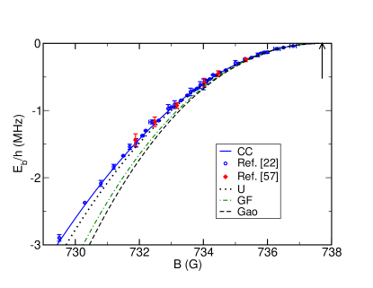
Figure 5: (Color online) Observed and calculated bound-state energies $E_{\mathrm{b}}$ in the (1,1) channel of ⁷Li as a function of magnetic field $B$: Coupled-channels calculation (solid line), experimental results from Refs. Dyke et al. (2013) (open circles) and Navon et al. (2011) (diamonds), and approximations from the universal (dotted), Gribakin-Flambaum (dot-dash) and Gao (dashed) formulas.

Figure 5 also shows the results of three simple single-channel formulas that relate the binding energy to the scattering length,

$$E^{\mathrm{U}}_{\mathrm{b}} = -\frac{\hbar^{2}}{2\mu a^{2}},$$ (13)

$$E^{\mathrm{GF}}_{\mathrm{b}} = -\frac{\hbar^{2}}{2\mu(a-\bar{a})^{2}},$$ (14)

$$E^{\mathrm{Gao}}_{\mathrm{b}} = -\frac{\hbar^{2}}{2\mu(a-\bar{a})^{2}}\left[1+\frac{g_{1}\bar{a}}{a-\bar{a}}+\frac{g_{2}\bar{a}^{2}}{(a-\bar{a})^{2}}\right],$$ (15)

where $g_{1}=\Gamma(1/4)^{4}/(6\pi^{2})\approx 2.9179$ and $g_{2}=(5/4)g_{1}^{2}-2\approx-0.9468$. The first formula is the familiar universal relationship between the last bound state and the scattering length Chin et al. (2010). The second gives a correction for the van der Waals potential that follows from the work of Gribakin and Flambaum Gribakin and Flambaum (1993). The final formula, due to Gao Gao (2004), includes higher-order corrections based on the analytic solutions of the Schrödinger equation for the van der Waals potential.

A good way to highlight the differences between the calculations, experimental results and approximate formulas is to plot $\epsilon r^{2}$ as a function of $1/r^{2}$, using van der Waals units of energy $\epsilon=E_{\mathrm{b}}/\bar{E}$ and length $r=a/\bar{a}$ . In these units the approximate formulas are

$$\epsilon^{\mathrm{U}}r^{2} = -1,$$ (16)

$$\epsilon^{\mathrm{GF}}r^{2} = \frac{-1}{\left(1-\frac{1}{r}\right)^{2}},$$ (17)

$$\epsilon^{\mathrm{Gao}}r^{2} = \frac{-1}{\left(1-\frac{1}{r}\right)^{2}}\left[1+\frac{g_{1}}{r-1}+\frac{g_{2}}{(r-1)^{2}}\right].$$ (18)

In this representation, the positions of the experimental points themselves depend upon the $a(B)$ mapping used to interpret them.

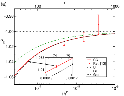
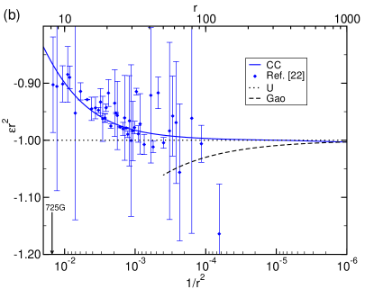
Figure 6: (Color online) Plots of $\epsilon r^{2}$ against $1/r^{2}$, using van der Waals units of energy and length. The solid lines show the coupled-channels calculation, the points give the experimental results mapped using the calculated $a(B)$ function evaluated at the measured $B$ values, and the dotted, dot-dash, and dashed lines give the results of the universal, Gribakin-Flambaum, and Gao formulas, respectively. (a) Bound-state energies in the (1,2) channel of ⁶Li, showing experimental results from Zürn et al. Zürn et al. (2013). The inset shows an expanded view near $1/r^{2}=0.00018$, or $a\approx 2200$ $a_{0}$. (b) Bound-state energies in the (1,1) channel of ⁷Li, showing experimental results from Dyke et al. Dyke et al. (2013).

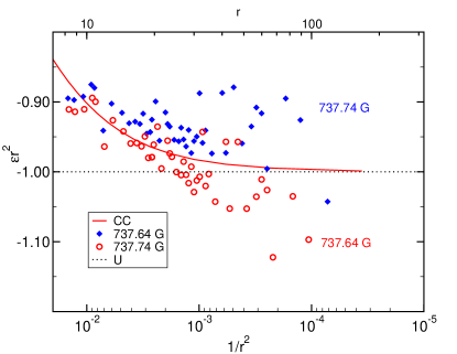
Figure 7: (Color online) Plots of $\epsilon r^{2}$ against $1/r^{2}$ in the (1,1) channel of ⁷Li, showing the experimental results of Dyke et al. Dyke et al. (2013), mapped with two different $a(B)$ functions calculated when the ${}^{1}\Sigma_{g}^{+}$ potential is adjusted slightly to give two different pole positions, 737.74 G and 737.64 G, which differ by $\pm 0.05$ G from our fitted value of 737.69(2) G.

Figure 6(a) compares the coupled-channels bound-state energies, the experimental results of Zürn et al. Zürn et al. (2013) and the three approximate formulas near the pole of the broad resonance in the (1,2) channel of ⁶Li. Even for this open-channel-dominated resonance with $s_{\mathrm{res}}\gg 1$, the universal formula differs from the coupled-channel bound-state energy by 3% at $1/r^{2}=0.0001$, or $a=100\bar{a}$. The Gribakin-Flambaum correction reduces the difference to about 1%, while Gao’s single-channel formula, Eq. (18), gives an excellent representation of the bound-state energy that differs from the coupled-channels result by only 0.06% at $1/r^{2}=0.0001$. Nevertheless, the measurement precision of ref. Zürn et al. (2013) is so good that the difference between the experimental results and the Gao formula reaches 5 times the experimental error of 0.02% near $1/r^{2}=0.00018$, or $a=74\bar{a}$, as shown in the inset of Fig. 6(a). The coupled-channels model, on the other hand, agrees with the measured value within experimental uncertainty. It may be noted that the universal value of $-1$ for $\epsilon r^{2}$ differs from the experimental value by nearly 200 times the experimental uncertainty for this point.

Figure 6(b) shows a similar comparison between the calculated bound-state energies and the experimental results of Dyke et al. Dyke et al. (2013) for the (1,1) channel of ⁷Li. There is much more scatter in the experimental results than for the ⁶Li results of Zürn et al., but the overall agreement with the coupled-channels model is good. The fluctuations in the experimental results near the pole are much more evident in this plot than in Fig. 5. It is also clear that the bound-state energies are quite poorly represented by Gao’s single-channel formula around this closed-channel-dominated resonance with $s_{\mathrm{res}}<1$. The apparent agreement with the universal formula over a wider range than for ⁶Li is an artifact, arising because, in the ⁷Li case, $\epsilon r^{2}$ deviates from its universal value of $-1$ in the opposite direction to that predicted by Gao’s single-channel formula.

Plotting measured values of $E_{\rm b}(B)$ as $\epsilon r^{2}$ against $1/r^{2}$ provides a sensitive test of the mapping $a(B)$ between magnetic field $B$ and scattering length $a$. In particular, if a mapping with an incorrect pole position is used, the results do not properly approach the limit $-1$ as $1/r^{2}\to 0$. Figure 7 shows this behavior for two coupled-channels models that have slightly incorrect pole positions, in this case differing by about $\pm 0.05$ G from our best value. It may be seen that the two sets of points clearly deviate from $-1$ in opposite directions as $1/r^{2}\to 0$. Such an error would be even more apparent in Fig. 6(a) if we plotted the recent experimental results of Zürn et al. Zürn et al. (2013) using the older $a(B)$ mapping from Bartenstein et al. Bartenstein et al. (2005). The points would then lie well off the coupled-channels and Gao curves, and the point nearest the pole would lie 10% away from the limiting value of $-1$ because of the 2 G difference in pole position between Bartenstein et al. and Zürn et al.

VI Conclusions

We have produced a new coupled-channels model for the collision of two cold Li atoms, based on published bound-state and scattering properties for both isotopic species ⁶Li and ⁷Li. Our new model simultaneously fits results for both isotopes to obtain ${}^{1}\Sigma_{g}^{+}$ and ${}^{3}\Sigma_{u}^{+}$ interaction potentials that include terms to account for the small mass-dependent corrections to the Born-Oppenheimer approximation. It is necessary to include such corrections for both the ${}^{1}\Sigma_{g}^{+}$ and ${}^{3}\Sigma_{u}^{+}$ potentials. Our calculations show the overall magnitude of the mass-correction effect through the difference in threshold phase for each of these potentials. Such constraints on the magnitude can be tested against theory if future ab initio studies determine the magnitude of the mass-dependent corrections to the Born-Oppenheimer approximation.

Our new model allows a careful study of the differences between three different approximate formulas that relate the binding energy of the Feshbach molecule to the scattering length of the two atoms. To do this, it is helpful to express the binding energy and scattering length in van der Waals units of $\bar{E}$ and $\bar{a}$. In these units, the conventional universal relationship predicts that the product of the bound-state energy and the square of scattering length has a constant magnitude $-1$, independent of species. Departures from this limit are readily apparent. Plotting the results in this way requires a mapping between the magnetic field $B$ and the scattering length $a$ and provides a sensitive test of the position of the resonance pole in $a(B)$. The high precision of measurement for ⁶Li₂ bound states and the quality of our coupled-channels model permit the differences between the experimental results and the approximate formulas to be seen clearly. Both the ⁶Li₂ and ⁷Li₂ bound states show pronounced departure from the universal formula as the binding energy increases away from resonance, even while the scattering length remains large compared to the characteristic van der Waals length. The two isotopologues show quite different patterns of variation away from the universal relationship, due to the large difference in their resonance pole strength $s_{\mathrm{res}}$. The binding energies near the strong ⁶Li resonance with $s_{\mathrm{res}}\gg 1$ agree well with the Gao relationship Gao (2004) for a single channel. However, those near the much weaker ⁷Li resonance with $s_{\mathrm{res}}<1$ are not well reproduced by any of the approximate formulas and require a coupled-channels model.