Additional Evidence Supporting a Model of Shallow, High-Speed Supergranulation

Abstract

Recently, Duvall and Hanasoge (Solar Phys. 287, 71-83, 2013) found that large distance $[\Delta]$ separation travel-time differences from a center to an annulus $[\delta t_{\rm{oi}}]$ implied a model of the average supergranular cell that has a peak upflow of $240\rm{\,m\,s^{-1}}$ at a depth of $2.3\rm{\,Mm}$ and a corresponding peak outward horizontal flow of $700\rm{\,m\,s^{-1}}$ at a depth of $1.6\rm{\,Mm}$. In the present work, this effect is further studied by measuring and modeling center-to-quadrant travel-time differences $[\delta t_{\rm{qu}}]$, which roughly agree with this model. Simulations are analyzed that show that such a model flow would lead to the expected travel-time differences. As a check for possible systematic errors, the center-to-annulus travel-time differences $[\delta t_{\rm{oi}}]$ are found not to vary with heliocentric angle. A consistency check finds an increase of $\delta t_{\rm{oi}}$ with the temporal frequency $[\nu]$ by a factor of two, which is not predicted by the ray theory.

1 Introduction

Supergranulation, first seen as a 30 Mm cellular pattern of horizontal flows detected by Doppler shifts [Hart (1954), Leighton, Noyes, and Simon (1962)] in the solar photosphere, continues to puzzle investigators (see review by Rieutord10). Recent work attempts to understand supergranulation by revealing its subsurface structure by numerical simulations [Stein et al. (2006)] or by local helioseismology [Gizon, Birch, and Spruit (2010)].

Detailed radiative-hydrodynamic simulations of the outer convection zone and atmosphere show no excess flow signal at the supergranular scale in the photosphere, in contrast to the observational results [Nordlund, Stein, and Asplund (2009)]. These simulations, which match the observations of the solar granulation so well, would seem to have all of the ingredients required to reproduce supergranulation. In particular, the early suggestion of Leighton62 that He II ionization could give rise to supergranulation, is tested by the simulations with a null result. One possibility remaining to be tested is the simulation of magnetic field, which is known to be present along cell boundaries.

Local helioseismology has been used extensively to study supergranulation (see review by Gizon10), although no consensus has emerged about fundamental questions such as the depth of the peak flow and the existence or not of counterflows at depth. Some efforts centered on making inversions of individual realizations of the supergranular flow field [Duvall et al. (1997), Zhao and Kosovichev (2003), Woodard (2007), Jackiewicz, Gizon, and Birch (2008), Švanda et al. (2012)]. In some of the work there is great difficulty in separating a horizontally diverging outflow from an upflow [Zhao and Kosovichev (2003), Dombroski et al. (2013)], although in other work this may have been solved [Švanda et al. (2012)]. To make flow maps of individual supergranular realizations, it has been necessary to restrict the measurements to small separations $[\Delta<5^{\circ}]$ for which the signal-to-noise ratio is large.

To measure the general properties of supergranulation, a large number of cells needs to be examined (in the present work, $6\times 10^{4}$ supergranules are analyzed). To increase the signal-to-noise ratio (S/N), spatial averages are made about cell locations determined from shallow signals such as peaks in the flow divergence. Such a method was first used by Birch06 and subsequently by Duvall10 and Svanda12. Weak signals can be separated cleanly from realization noise, although more attention to systematic errors is required. As noticed by Svanda12, the present method of defining cells is probably biased towards larger cells than the average. This might be corrected (in the future) by directly modeling the spatial autocovariance of the travel-time maps.

The averaging of the signals from many cells makes it possible to use larger $\Delta$s (up to $24^{\circ}$ in the present study), which would normally not be feasible for a 12-hour observation because of the increased noise due to the amplitude reduction from the geometrical spreading of the wavefront [Gizon and Birch (2004)]. The separation of the horizontal and vertical flow signals is much better at larger $\Delta$, as the rays are more vertical in the critical near-surface region. Duvall13 (hereafter Article I) found that the center-to-annulus travel-time difference $[\delta t_{\rm{oi}}]$ was roughly constant at $5.1$ seconds in the range $\Delta=10-25^{\circ}$. In a simple ray-theory interpretation, this requires a vertical upflow considerably larger than the $10\rm{\,m\,s^{-1}}$ observed at the photosphere [Duvall and Birch (2010)] and in fact the best-fit model had a peak upflow of $240\rm{\,m\,s^{-1}}$ at $z=-2.3\rm{\,Mm}$. Plots of this model and the bracketing models are shown in Figure F-flowmodels. That large vertical upflows are required was recently confirmed by the analysis of Svanda12 by a considerably different formalism.

The strategy for obtaining the best model was developed in Article I and is as follows: We assumed the simplest vertical-flow model that reduces to a $10\rm{\,m\,s^{-1}}$ vertical flow at the surface and still approaches the $5.1$ seconds for the asymptotic behavior of the $\delta t_{\rm{oi}}$ signal at large $\Delta$. This is the gaussian with a single peak. For a particular choice of depth of the peak vertical flow $[z_{0}]$, the width of the gaussian and its amplitude are determined uniquely by the $5.1$ seconds $\delta t_{\rm{oi}}$ signal requirement and the $10\rm{\,m\,s^{-1}}$ upward flow at the photosphere. With some reasonable choices for the horizontal parameters $k$ and $R$ (see Article I), the horizontal flow is then determined from the vertical flow and the continuity equation. Three models were examined that bracket the observations. These are distinguished by the height of the peak flow, $z_{0}=-1.15\rm{\,Mm}$, $z_{0}=-2.30\rm{\,Mm}$, and $z_{0}=-3.45\rm{\,Mm}$. The $\delta t_{\rm{oi}}$ signal is computed from the ray theory using both the vertical and horizontal flow components. We found that the $z_{0}=-2.30\rm{\,Mm}$ model was most similar to the observations. For the $z_{0}=-3.45\rm{\,Mm}$ model (and any with a deeper $z_{0}$), the horizontal component contributes significantly and leads to a behavior at large separations that is inconsistent with the observations. We conclude that if there is a deeper horizontal flow, it must have a small magnitude to not be observed in the $\delta t_{\rm{oi}}$ signal.

In the present work, the efforts of Article I are extended to include quadrant analysis in Section sec-quad, an attempt to measure a heliocentric-angle (or center-to-limb) dependence in Section sec-heliocen, tests with simulations in Section sec-sim, and an attempt to measure a temporal-frequency $[\nu]$ dependence in Section sec-nu. We give some conclusions in Section sec-dis.

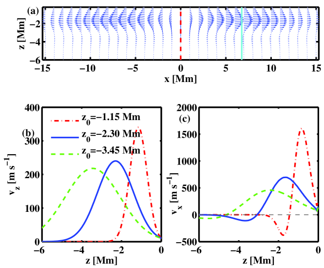
Figure 1.: The flow models from Article I. (a) Velocity vectors for the best model. This is the model labeled g2 in Table 1 of Article I, with peak upward flow of $240\rm{\,m\,s^{-1}}$ at $z=-2.3\rm{\,Mm}$ and peak horizontal flow of $700\rm{\,m\,s^{-1}}$ at $z=-1.6\rm{\,Mm}$ and $x=7\rm{\,Mm}$. The cuts shown in (b) are taken at the location of the red dashed vertical line in (a). The cuts in (c) are taken at the location of the turquoise line in (a) at $x=7\rm{\,Mm}$. (b) Cuts of the vertical flow at cell center for the three models in Article I, model g1 (green; dashed), model g2 (blue; solid), and g3 (red; dot-dashed). (c) Cuts of the horizontal flow versus height at the location of the peak flow. Colors and line styles are the same as in (b). F-flowmodels

2 Analysis

2.1 Quadrant Analysis

sec-quad In Article I it was shown that the center–annulus travel-time difference $[\delta t_{\rm{oi}}]$ at large distances $[\Delta]$ is mostly sensitive to the supergranular vertical-flow signal. We might expect that at large $\Delta$ that the center-to-quadrant signals $[\delta t_{\rm{qu}}]$, where $qu$ corresponds to the West–East and North–South quadrant signals $[\delta t_{\rm{we}}$ and $\delta t_{\rm{ns}}]$, would be mostly sensitive to the horizontal supergranular flow. To test this idea, travel-time difference maps were constructed with ray-theory modeling of the average supergranule-flow model g2 from Article I. The results are shown in Figure F-model_cuts with the horizontal, vertical, and sum flow contributions to the travel time differences shown separately. For these relatively large $\Delta$s of $11.76^{\circ}$ and $20.64^{\circ}$, the center–annulus time differences $[\delta t_{\rm{oi}}]$ show very little contribution to the peak signal from the horizontal flow (relative magnitude 0.008 for $\Delta=11.76^{\circ}$ and 0.001 for $\Delta=20.64^{\circ}$). The contribution of the vertical signal to the peak $\delta t_{\rm{we}}$ is a little larger (0.064 for $\Delta=11.76^{\circ}$ and 0.050 for $\Delta=20.64^{\circ}$), but still small. Therefore the center–annulus differences $[\delta t_{\rm{oi}}]$ and quadrant directional differences $[\delta t_{\rm{qu}}]$ do separate the vertical and horizontal contributions quite well, if the ray theory can be believed. It would be very difficult to construct a model with these responses in which the horizontal flows are leaking into the $\delta t_{\rm{oi}}$ signal to yield the five-second signal at large $\Delta$.

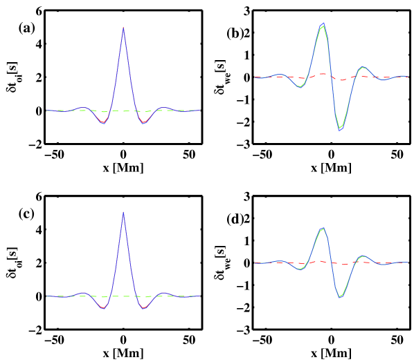
Figure 2.: Cuts in the east–west direction across model maps for center–annulus travel time differences $[\delta t_{\rm{oi}}]$ ((a) and (c)) and west–east travel-time differences $[\delta t_{\rm{we}}]$ ((b) and (d)) for distances $\Delta=11.76^{\circ}$ ((a) and (b)) and $\Delta=20.64^{\circ}$ ((c) and (d)). Vertical-flow contributions to the travel times are in red (solid in (a) and (c); dashed in (b) and (d); horizontal contributions are in green (dashed in (a) and (c); solid in (b) and (d)); and the sum is in blue. The model is the nominal one from Article I (g2) in which the peak upward vertical flow is at a depth of $2.3\rm{\,Mm}$ with magnitude of $240\rm{\,m\,s^{-1}}$. The peak horizontal flow is at a depth of $1.6\rm{\,Mm}$ at a distance $7\rm{\,Mm}$ from cell center and with velocity $700\rm{\,m\,s^{-1}}$. In general it is very difficult to separate the sum signal (blue) from the dominant signal (vertical flow (red) in (a) and (c) and horizontal flow (green) in (b) and (d)). F-model˙cuts

To compare the quadrant signals with the models, Helioseismic and Magnetic Imager (HMI) data were analyzed as in Article I with some improvements. The same 64 12-hour intervals (10 June 2010-10 July 10 2010) were analyzed with the same constant degree–width filter with width $\Gamma_{\rm{\ell}}=400$. Cross-correlation maps were constructed for each 12-hour period for the in and out-annulus signals and for the four quadrant signals (eastward, etc. direction of waves) for the 14 distance ranges of Article I and two additional ones at small $\Delta$ (centered at $1.20^{\circ}$ and $1.44^{\circ}$). The coordinate system used has equal increments in longitude and latitude of $0.24^{\circ}$. Gizon–Birch travel times [Gizon and Birch (2004)] were computed for each set of cross correlations and the desired differences: $\delta t_{\rm{oi}}$, $\delta t_{\rm{we}}$, and $\delta t_{\rm{ns}}$. The reference correlation was taken as the average over the in and out correlations averaged over the map, which is of size $96.24^{\circ}$ on a side. An average of these travel-time differences is made about the supergranular centers. In this average, the latitude–longitude travel-time difference maps are transformed locally to a Postel’s coordinate system centered on the feature. In this way, features at different latitudes are treated equally and the resultant average maps can be compared more readily with theory. Note that this was not the case in Article I, where the averages about the feature locations were done in the latitude–longitude coordinate system. However, as only the center of the maps where the peak $\delta t_{\rm{oi}}$ signal was obtained were used, it was acceptable. The supergranular-averaged 12-hour maps are averaged over the 64 different intervals. One advantage of doing the analysis in this way is that an estimate of the error can be made at each map location from the scatter of the 64 different intervals. One might imagine that the scatter would be larger where the average signal is larger just because of the variability in the supergranular signal. However, this was not the case, and the maps of errors showed no distinguishable features.

Some background signals are removed from these superposed images before further analysis. The $\delta t_{\rm{oi}}$ signal approaches a nonzero constant far from the central feature. This constant is measured and removed for each $\Delta$ range from the overall image as in Article I. The $\delta t_{\rm{we}}$ signal has a relatively large constant (six seconds for the smallest $\Delta$ to one second for the largest) removed. This signal is due to the average rotation over the field. This signal could be reduced by adjusting the tracking rate from the nominal Carrington rate. The $\delta t_{\rm{ns}}$ signal has both constant offsets and slopes in the North–South direction at different distances $[\Delta]$. The magnitudes are generally small ($<$ one second), but they are present in the background and hence were removed. Of these signals subtracted, only the rotation one is well understood.

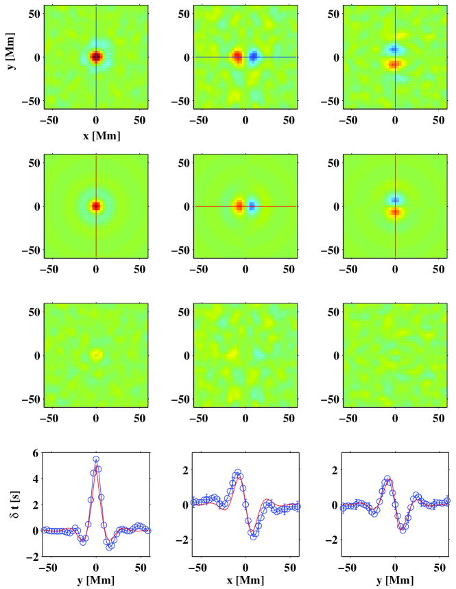
Figure 3.: Comparison of data with models for the distance range $\Delta=19.1$ – $22.2^{\circ}$. The first column is the center–annulus travel time difference $[\delta t_{\rm{oi}}]$, The second column is the quadrant West–East travel time difference $[\delta t_{\rm{we}}]$ and the third column is North–South $[\delta t_{\rm{ns}}]$. The top row is for the data 32-day average of all supergranules. The second row is the model and the third row is the difference of data minus model. The fourth row are cuts through the data and model images with data shown as blue (with symbols) and model as red. Where the cuts are taken is shown by the lines across the maps in the top two rows. The color scales of the images are in a spectral sequence with the first column covering -5 [seconds] for blue and +5 [seconds] for red. This is reduced in the second and third columns to -3 [seconds] for blue and +3 [seconds] for red. The dominant blue-green color corresponds to 0 [seconds]. The observed images are made antisymmetric in x about the center point in the middle column and antisymmetric in y about the center point in the right column. F-cmp˙model

Comparisons between models and data are shown in Figure F-cmp_model for the 15th (of 16) distance range ($\Delta=19.1$ – $22.2^{\circ}$). $\delta t_{\rm{oi}}$ are shown in the left column, $\delta t_{\rm{we}}$ in the middle column, and $\delta t_{\rm{ns}}$ in the right column. The 32-day average data are shown in the top row; model g2 from Article I images are shown in the second row; and the residual (data – model) are shown in the third line from the top. The fourth line shows cuts across important parts of the data and model images. In general, there is good agreement between the data and the ray theory modeling. The only apparent systematic difference between the data and the model is in the $\delta t_{\rm{oi}}$ signal near the center. It would seem that the width or amplitude of the model could be slightly adjusted.

One might imagine that if the five-second peak signal in $\delta t_{\rm{oi}}$ were due to an incorrect kernel, that the quadrant signals might be very different from the predicted. However, this is not the case. It does not preclude the possibility that at these large separations all of the ray kernels are multiplied by some factor. Birch07 have found a case where the ray kernel is a factor of two larger than the Born-approximation kernel, although this was at small $\Delta$ and for the fundamental $f-$mode.

To compare the $\delta t_{\rm{we}}$ and $\delta t_{\rm{ns}}$ signals with model predictions, the quadrant signals are characterized by the peak signal in the cuts shown in Figure F-cmp_model. Once the maximum signal is found, the neighboring two points are used to compute a parabola to refine the value of the maximum. Model travel-time images are treated the same way as the data. The three models from Article I are compared with the peak quadrant signals in Figure F-wens_vs_model. At the upper half of the $\Delta$ range, the observed signals agree pretty well with the model with peak vertical flow at depth $2.30\rm{\,Mm}$, the same model that agreed best with the $\delta t_{\rm{oi}}$ signal in Article I. At shorter $\Delta$, the observed signals deviate significantly from that model and agree better with the more shallow model with peak vertical flow at depth $1.15\rm{\,Mm}$. Either the precise form of the model is not right or the kernels are incorrect.

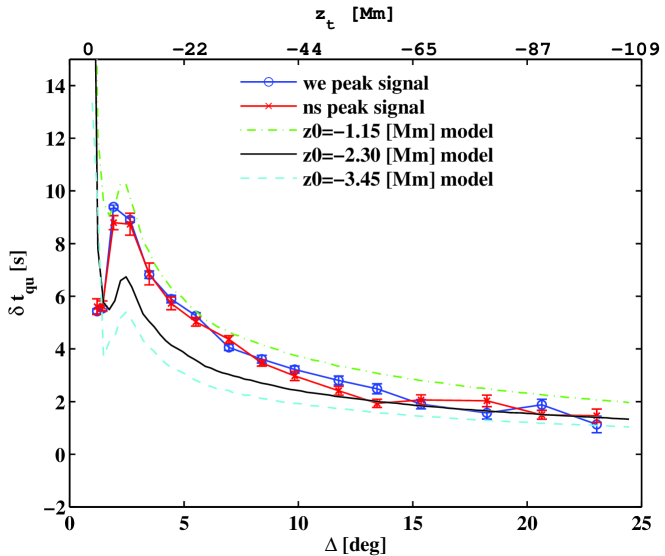
Figure 4.: Measured West–East and North–South quadrant peak travel-time differences $[\delta t_{\rm{qu}}]$ versus those from the three models from Article I. The blue symbols and error bars (hardly visible) are for the $\delta t_{\rm{we}}$ and the red for the $\delta t_{\rm{ns}}$. The central model (black) is the one that agreed best with the $\delta t_{\rm{oi}}$ signal. $z_{0}$ is the height of the peak vertical flow. On the bottom axis is shown the separation between center and quadrant $[\Delta]$ and on the top axis the corresponding turning point depth $[z_{t}]$. F-wens˙vs˙model

2.2 Heliocentric Angle Analysis

sec-heliocen Recently it has been found that there are flow artifacts with a center-to-limb, or heliocentric angle $[\theta]$ dependence [Zhao et al. (2012)]. As the center–annulus travel time difference $[\delta t_{\rm{oi}}]$ of $5.1\pm 0.1\rm{\,seconds}$ at distances $\Delta>10^{\circ}$ is a somewhat surprising signal, it was decided to check whether there is any $\theta$-dependence, which would indicate an artifact. This is done by separating the different supergranules into 11 bins based on the heliocentric angle of the cell center at the central observation time. The bins were chosen to give roughly equal numbers of features in each bin to attempt to equalize the errors from the different bins.

The analysis follows the quadrant analysis in Section sec-quad, except that when the average cross correlations are computed about the supergranular centers, there are 11 averages computed for the different $\theta$ bins.

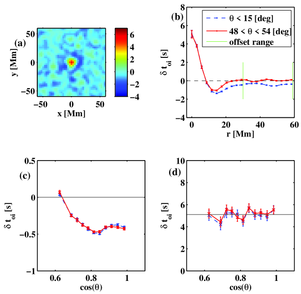
Figure 5.: (a) Center–annulus travel-time difference averaged about supergranule centers for the range of $\Delta=14.4$ – $24^{\circ}$ for heliocentric angle $\theta<15^{\circ}$. The scale of the colorbar at right is in seconds. (b) Azimuthal average of (a) (blue; dashed) and for $\theta=48$ – $54^{\circ}$ (red; solid). The range $r=30$ – $60\rm{\,Mm}$ over which the offset is averaged is noted by the vertical green lines. Note the offset at large radii that is smaller (in absolute value) at large $\theta$. This offset is believed to be an artifact which needs to be removed from the results. (c) The offset at $r=30$ – $60\rm{\,Mm}$ for the different travel-time definitions versus $\cos(\theta)$. Blue (dashed) is for the Gabor wavelet phase time differences. Red (solid) is for the Gizon–Birch phase time differences. (d) The resultant travel time differences averaged for the 64 12–hour datacubes corrected for the offset in (c) versus $\cos(\theta)$. The colors are the same as in (c). In (a) – (d) distances were averaged over the range $\Delta=14.4$ – $24^{\circ}$. F-tt˙rho

Gizon–Birch travel times are computed for each 12-hour interval and the results from the 64 intervals are averaged. The reference correlation was taken as the average over the in and out correlations averaged over the superposed map, which is of size $9.84^{\circ}$ on a side. There is thus a separate reference correlation for each $\theta$ bin. This is important as the reference correlation varies from center to limb, and if it is not taken into account, spurious results are obtained. With the 11 bins in heliocentric angle, there was insufficient S/N ratio to compute Gabor-wavelet times for the individual 12-hour intervals. So, the correlations from the 64 12-hour intervals were averaged and the Gabor wavelets were fit to the result. With the travel-time differences computed in this way, the Gabor wavelet and Gizon–Birch times are almost identical. This should not be too surprising as the same correlation windows are fit in the two cases. Even the noise in the resultant travel-time difference maps is highly correlated.

Results for the center–annulus travel-time difference $[\delta t_{\rm{oi}}]$ are presented in Figure F-tt_rho. The average Gabor-wavelet-phase time difference for the first bin ($\theta<15^{\circ}$) and for the distance range $\Delta=14.4$ – $24^{\circ}$ is shown in Figure F-tt_rhoa. The normal large positive signal of $\approx$ five seconds is seen at cell center surrounded by a negative moat with signal $\approx-$one $\rm{\,seconds}$ corresponding to the region of downflow of the average cell and also the downflow for neighboring cells. The overall mottling of the picture has roughly supergranular scale and is presumably due to incomplete averaging of the supergranular field. To get a better indication of the average signal, which we expect to be azimuthally symmetric about cell center, an azimuthal average of the signal in Figure F-tt_rhoa is shown in Figure F-tt_rhob (blue;dashed). Also shown in Figure F-tt_rhob in red (solid) is the azimuthal average signal in the outer $\theta$ bin.

We would expect a zero signal far from cell center. That it is not, at least for the inner $\theta$ bin, is apparent in Figure F-tt_rhob. This signal, which we measure as the average on $r=30$ – $60\rm{\,Mm}$, is shown in Figure F-tt_rhoc for Gabor-wavelet fitting (blue;dashed) and Gizon–Birch times (red;solid). The variation with $\cos{\theta}$ suggests that this signal is an artifact that could safely be used to correct the signal at cell center. It may be related to the center-to-limb flow artifact reported by Zhao12, as a cell center at disk center will see a $\delta t_{\rm{oi}}$ of roughly the magnitude shown for the annulus radii used here.

The results in Figure F-tt_rhoc are subtracted from the cell center signal to yield the corrected cell center signal in Figure F-tt_rhod. Again the Gabor-wavelet times and the Gizon–Birch times are very close and in addition, no significant center-to-limb signal is apparent. Fitting a line to the results yields a slope with an error about equal to the value. The average over $\theta$, $5.1\rm{\,seconds}$, is consistent with the results of Article I.

2.3 Simulations

sec-sim In Article I, a convectively stabilized solar model [Hanasoge and Duvall (2006)] was used with vertical-flow features with flow peaking at a depth of $z_{0}=-2.3\rm{\,Mm}$ with Gaussian depth profile with width $\sigma_{z}=0.82\rm{\,Mm}$ and horizontal Gaussian width $\sigma_{h}=5.1\rm{\,Mm}$. A global simulation of wave propagation is performed with wave sources near the surface [Hanasoge, Duvall, and Couvidat (2007)]. Center to annulus travel-time differences $[\delta t_{\rm{oi}}]$ were measured from the simulation results as a function of the annulus radius $[\Delta]$. To obtain travel times similar to the observed $5.1\rm{\,seconds}$ required the peak amplitude of the Gaussian flow to be $338\rm{\,m\,s^{-1}}$. Ray-theory calculations were made and we found that the $\delta t_{\rm{oi}}$ for the ray theory were 24 % larger, suggesting some problem. However, we had used the standard Model S [Christensen-Dalsgaard et al. (1996)] to do the ray-theory calculations where we should have been using the convectively stablilized model, which it turns out makes a significant difference. A revised version of Figure 2 of Article I is shown in Figure F-sim_vert. On the distance range $10$ – $24^{\circ}$, the average measured travel-time difference $[\delta t_{\rm{oi}}]$ is now very close to the ray-theory prediction. This result shows that vertical flows like the ones suggested in Article I are correctly modeled by the ray theory, as long as one is using the correct background model. It does not tell us, however, what might happen to the corresponding horizontal flows and whether the separation of horizontal and vertical flows by the $\delta t_{\rm{oi}}$ and $\delta t_{\rm{qu}}$ is valid.

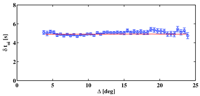
Figure 6.: Comparison of the center–annulus travel-time differences $[\delta t_{\rm{oi}}]$ from the linear simulation (blue with symbols) with the travel-time difference computed from the ray theory with the same flow perturbations (red line). The model used in the ray-theory computation is the convectively stablized one used in the simulation. The error bars are computed from the scatter far from the feature locations. No filtering has been done before the travel-time measurements. The average travel-time difference in the range $\Delta=10$ – $24^{\circ}$ has been scaled to match the observationally determined mean $5.1\rm{\,seconds}$. The same scaling factor is then used to scale the ray-theory results. F-sim˙vert

To test whether the horizontal- and vertical-flow components are separated by the measurements of $\delta t_{\rm{oi}}$ and $\delta t_{\rm{qu}}$, a simulation was done using a flow model identical to model g2 of Article I. The solar model used is the convectively stabilized one described above and a Cartesian simulation is done using the SPARC code (Hanasoge06b,2008;Hanasoge06). 500 features identical to the flow in model g2 are placed randomly in the horizontal plane. Center–annulus and quadrant travel-time differences are measured as described above. The horizontal spacing of the simulation is $5.7\rm{\,Mm}$ with $512\times 512$ pixels. The maximum depth is $104\rm{\,Mm}$. The attempt was to go as deeply as possible in order to be able to use large distances. In order to be able to put the 500 features over the entire horizontal field and still be able to obtain full annulus coverage for large separations, the horizontal periodicity of the simulation was used in the travel-time computation.

The travel-time differences from the simulation and ray-theory computations are shown in Figure F-sim_oiwe. The travel-time differences are only shown up to $\Delta=13^{\circ}$, as the simulation was not deep enough to go to larger $\Delta$. The $\delta t_{\rm{oi}}$ measurements in Figure F-sim_oiwea seem noisier than expected from the error bars. There is a rough agreement with the ray theory. The asymptotic limit at $\Delta=24^{\circ}$ is only $3.1\rm{\,seconds}$, as opposed to the expected $5.1\rm{\,seconds}$. This is because in the convectively stabilized model the sound speed is modified, which affects the ray-theory estimate of the travel-time differences in the integral $\int{{\rm dr}(v/c^{2})}$. There is less general agreement of the quadrant travel-time differences with the ray theory. Especially for $\Delta<5^{\circ}$, the ray theory is predicting too large a travel-time difference, while for $\Delta>10^{\circ}$ the opposite may be the case.

For both the spherical simulation (Figure F-sim_vert) and for the Cartesian one (Figure F-sim_oiwea), the ray theory has general agreement with the $\delta t_{\rm{oi}}$ measured from the simulations. This suggests that the ray theory can adequately predict $\delta t_{\rm{oi}}$ for the range of $\Delta$ examined and for flows at this depth of $z=-2.3\rm{\,Mm}$. For the quadrant travel times, the situation is more problematic. One question is whether a more shallow flow peaking at the surface could somehow have its quadrant signal mimic the $\delta t_{\rm{oi}}$ signal of $5.1\rm{\,seconds}$. This will need to wait for future work.

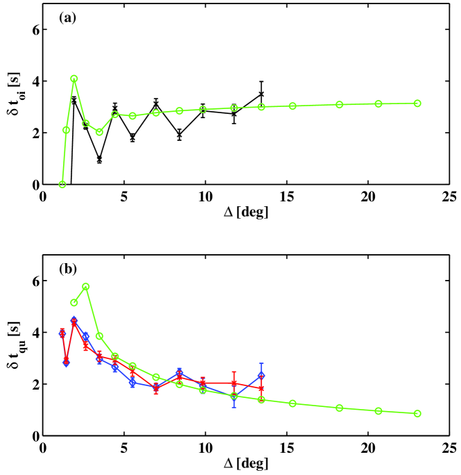
Figure 7.: Comparison of travel-time differences measured from a simulation with ray-theory computations. (a) Center-annulus travel-time differences $[\delta t_{\rm{oi}}]$ from the simulation (black with crosses, error bars, and connecting lines) and ray-theory computations of $\delta t_{\rm{oi}}$ (green circles). (b) Quadrant travel-time differences $\delta t_{\rm{we}}$ (blue diamonds) and $\delta t_{\rm{ns}}$ (red crosses) for the simulation and ray-theory computations for $\delta t_{\rm{we}}$ (green circles). F-sim˙oiwe

2.4 Travel Times Versus Temporal Frequency $[\nu]$

sec-nu Another way to test the validity of the ray theory applied to flow measurements is to measure the travel times versus the temporal frequency $[\nu]$. To first order, at the same distance $\Delta$, the travel-time differences due to flows should be constant, according to the ray theory. To our knowledge, such a test has not been carried out, although the frequency dependence of travel times has been measured extensively, e.g. Dombroski13. For the ridge filtering used in that study, a $\nu$-dependence is expected, however. Such a test was conducted for the 64 12-hour intervals at the largest distance range used, $\Delta=22.1$ – $24^{\circ}$. The travel-time results versus $\nu$ are shown in Figure F-vs_freq.

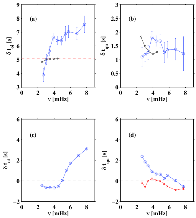
Figure 8.: Peak signals and backgrounds versus the temporal frequency $[\nu]$ for the largest distance band $\Delta=22.1$ – $24^{\circ}$. (a) The center–annulus travel-time difference $[\delta t_{\rm{oi}}]$ versus the temporal frequency $[\nu]$ (blue circles). The red horizontal dashed line is at $5.1\rm{\,seconds}$, the result for the $\nu$-averaged data. The black crosses and line are ray-path calculations based on model g2 from Article I. (b) The peak quadrant travel-time difference $[\delta t_{\rm{qu}}]$ (blue cirlces), where the $\delta t_{\rm{we}}$ and $\delta t_{\rm{ns}}$ signals have been averaged to reduce the error bar size. The red horizontal dashed line is at the value for the $\nu$-averaged result, $1.3\rm{\,seconds}$. The black crosses and curve are ray-path calculations based on model g2 from Article I. (c) The center–annulus background signal far from the supergranule centers versus $\nu$ (blue circles). This signal was subtracted from the observed signal to yield the result in (a). The dashed black line indicates zero. (d) The background signals for $\delta t_{\rm{we}}$ (blue circles) and $\delta t_{\rm{ns}}$ (red crosses). These were subtracted from the observed signals and then the $\delta t_{\rm{we}}$ and $\delta t_{\rm{ns}}$ were averaged to yield the result in (b). The dashed black line indicates zero. F-vs˙freq

To obtain these results, the datacubes were filtered as before with the phase-speed filter with constant degree width $\Gamma_{\ell}=400$, and in addition a frequency filter. Ten separate frequency filters were used. The first seven had central frequencies from $\nu=2.5\rm{\,mHz}$ to $\nu=5.5\rm{\,mHz}$ in steps of $0.5\rm{\,mHz}$ with power full width at half maximum of $0.5\rm{\,mHz}$. The last three filters had central frequencies of $\nu=6,7,8\rm{\,mHz}$ with power full width at half maximum of $1.0\rm{\,mHz}$. Center–annulus and quadrant cross-correlation maps were constructed for each of the 64 12-hour intervals. Average correlations were used to measure guess times for the different $\nu$ intervals. Gizon–Birch travel-time maps were computed for the 64 intervals and the results were averaged over $\Delta$ and the various differences computed. Average maps about the supergranulation centers were made. Background signals were measured far from the central feature for each $\nu$ for the different signals. These are shown in Figure F-vs_freqc and F-vs_freqd. These are subtracted from the peak signals observed to yield the results for $\delta t_{\rm{oi}}$ in Figure F-vs_freqa and for the two quadrant signals subsequently averaged to yield Figure F-vs_freqb.

The center–annulus travel time differences $[\delta t_{\rm{oi}}]$ in Figure F-vs_freqa are clearly not constant with frequency but increase by a factor of $\approx$two over the $\nu$ range. For $\nu<\nu_{\rm ac}$, where $\nu_{\rm ac}\approx 5\rm{\,mHz}$ is the peak acoustic-cutoff frequency of the atmosphere, the variation is approximately linear with a zero intercept. For $\nu>\nu_{\rm ac}$, the increase with frequency is somewhat smaller. There have not been any predictions of flow travel times for $\nu>\nu_{\rm ac}$, but it was feasible to measure them, and so it was done. Ray-theory calculations of the travel-time differences are also shown in Figure F-vs_freqa and Figure F-vs_freqb. This result casts some doubt on the simple interpretation of the $\delta t_{\rm{oi}}$ measurements in terms of the ray theory. The acoustic-cutoff frequency used in the ray calculations is Lamb’s definition $\omega_{c}=c/2H_{p}$ Lamb (1909), where $c$ is the sound speed and $H_{p}$ is the pressure scale height. It is interesting that the peak quadrant travel times $[\delta t_{\rm{qu}}]$ in Figure F-vs_freqb are approximately constant over the $\nu$ range, although with a mean signal of $1.3\rm{\,seconds}$, the uncertainty in this conclusion is large. The ray-theory estimates are consistent with the measurements for the quadrant travel times.

The background signal for the $\delta t_{\rm{oi}}$ shown in Figure F-vs_freqc is very interesting. It is measured far from the central location, but is basically consistent with taking the average signal over a large area. In the trapped mode region $[\nu<\nu_{\rm ac}]$, the signal is relatively small and negative, while for $\nu>\nu_{\rm ac}$, it becomes positive and increases with $\nu$. We have no particular hypothesis for the source of this signal, but this additional information on the $\nu$ variation may be important for understanding it. The background for the quadrant signals $[\delta t_{\rm{we}}$ and $\delta t_{\rm{ns}}]$ are shown in Figure F-vs_freqd. These signals are measured far from the central location in the North–South direction for the $\delta t_{\rm{we}}$ and in the West–East direction for the $\delta t_{\rm{ns}}$ signal. The $\delta t_{\rm{we}}$ signal has a linear variation over the frequency range. This background signal is possibly due to solar rotation, although it would imply that the solar rotation yields a $\nu$-dependent $\delta t_{\rm{we}}$ while the supergranular signal does not. Whatever causes background signals, they need to be removed from the supergranular signal.

3 Conclusions

sec-dis

The bulk of the evidence in the present article continues to support a model of the average supergranulation cell as having an upflow with a velocity much larger than the surface upflow of $10\rm{\,m\,s^{-1}}$, possibly as large as $240\rm{\,m\,s^{-1}}$ and a peak flow $2$ – $3\rm{\,Mm}$ below the surface as seen in the best model g2. In Article I, center–annulus travel time differences $[\delta t_{\rm{oi}}]$ were shown to agree well with model g2, while in the present article, the quadrant travel-time differences $[\delta t_{\rm{we}}$ and $\delta t_{\rm{ns}}]$ also agree mostly with this type of model. However, there is some disagreement that varies with $\Delta$ for the $\delta t_{\rm{qu}}$, suggesting that either the functional form of the model needs to be adjusted or the ray kernels are incorrect, or both.

The apparent disagreement between the present work and the smaller flows seen before has largely disappeared with the work of Svanda12. That article does an analysis of average supergranules similar to the averaging done in the present article. He used $f$-modes and small separation p-modes and finds flows that largely confirm the present results. There may be a factor of two difference between the two results, which needs to be resolved.

The lack of a center-to-limb variation of the $\delta t_{\rm{oi}}$ signal is useful for a general check of systematic errors. However, the $\nu$-dependence of the $\delta\tau_{\rm oi}$ signal as predicted by ray theory differs from observations, suggesting that ray theory may be inaccurate in near-surface layers. The errors may be due to unmodeled finite-frequency effects or possibly differences in the acoustic-cutoff frequency between the Sun and Model S (used in ray modelling here). That the acoustic-cutoff frequency may differ from that derived from Model S was shown by Jefferies94. In a model with the reflection point that is a significant function of frequency, the travel-time difference $[\delta t_{\rm{oi}}]$ could then also be a function of frequency. At a minimum, the variation in $\delta t_{\rm{oi}}$ by a factor of roughly two over the $\nu$-range observed would seem to make the suggested flows uncertain by a similar factor.

The simulation results (Section sec-sim) show that the type of model considered (model g2) does induce the kind of travel-time shifts observed. These are then seen by both the travel-time shifts measured from the simulation and by ray theory calculated with the model used. It is unfortunate that the modification to the solar model to stablize it has such a large effect on the resulting $\delta t_{\rm{oi}}$.

Some of the earlier work finds the flow velocity peaking very near the surface with a monotonic decrease with depth Birch et al. (2006); Woodard (2007). These results would appear to be inconsistent with this article and Article I. It was suggested in Article I that the perturbations to the p-mode spectrum due to supergranulation are significant in $\ell$, the spherical-harmonic degree. The idea is that the supergranulation pattern, with a spectrum peaking near $\ell=120$ would induce a modulation of a $p$-mode ridge that would have a width in $\ell$ of at least twice this amount. To capture all of the supergranulation signal requires a filter of at least a full-width-half-max of $\Gamma_{\ell}=240$ and likely larger. This justifies the value chosen for the present work of $\Gamma_{\ell}=400$, which clearly captures all of the $\delta t_{\rm{oi}}$ signal at large $\Delta$. This conclusion is supported by Figure 4 of Article I. Of course, if the modeling is correct, one can use any filter. However, if much of the supergranulation signal is not being captured, one becomes much more sensitive to the modeling. In Woodard07, the filters are narrower than used here, particularly at low frequencies.

Because the acoustic wavelength at the depth of the peak flow is larger than the depth of the peak flow, ray theory may show inaccuracies. To improve the quality of the flow model, it would therefore be useful to include finite-frequency effects Birch and Gizon (2007). Further, the functional dependence of travel times on the background-flow model may exceed the linear limit if flow speeds are indeed on the order of $700\rm{\,m\,s^{-1}}$. Therefore a non-linear inversion for supergranular flow may be necessary to explain the measured travel times Hanasoge et al. (2011).

Acknowledgements

The data used here are courtesy of NASA/SDO and the HMI Science Team. We thank the HMI team members for their hard work. This work is supported by NASA SDO.

References

- Birch and Gizon (2007) Birch, A.C., Gizon, L.: 2007, Astronomische Nachrichten 328, 228.
- Birch et al. (2006) Birch, A., Duvall, T.L. Jr., Gizon, L., Jackiewicz, J.: 2006, Bull. of the Am. Astronom. Soc. 38, 224.
- Christensen-Dalsgaard et al. (1996) Christensen-Dalsgaard, J. et al.: 1996, Science, 272, 1286.
- Duvall and Birch (2010) Duvall, T.L. Jr., Birch, A.C.: 2010, Astrophys. J. Lett. 725, L47.
- Duvall and Hanasoge (2013) Duvall, T.L. Jr., Hanasoge, S.M.: 2013, Solar Phys. 287, 71. ADS, DOI. (Article I)
- Dombroski et al. (2013) Dombroski, D. E.; Birch, A. C.; Braun, D. C.; Hanasoge, S. M.: 2013, Solar Phys. 282, 361. ADS, DOI.
- Duvall et al. (1997) Duvall, T.L. Jr., Kosovichev, A.G., Scherrer, P.H., Bogart, R.S., Bush, R.I., deForest, C., Hoeksema, J.T., Schou, J., Saba, J.L.R., Tarbell, T.D., Title, A.M., Wolfson, C.J., Milford, P.N.: 1997, Solar Phys. 170, 63. ADS, DOI.
- Gizon and Birch (2004) Gizon, L., Birch, A.C.: 2004, Astrophys. J. 614, 472.
- Gizon, Birch, and Spruit (2010) Gizon, L., Birch, A.C., Spruit, H.C.: 2010, Ann. Rev. Astron. Astrophys. 48, 289.
- Hanasoge and Duvall (2006) Hanasoge, S.M., Duvall, T.L. Jr.: 2006, in: Fletcher, K., Thompson, M. eds., Proceedings of SOHO 18/GONG 2006/HELAS I, Beyond the spherical Sun, ESA SP-624, 40.1.
- Hanasoge, Duvall, and Couvidat (2007) Hanasoge, S.M., Duvall, T.L. Jr., Couvidat, S.: 2007, Astrophys. J. 664, 1234.
- Hanasoge et al. (2006) Hanasoge, S.M., Larsen, R.M., Duvall, T.L. Jr., De Rosa, M.L., Hurlburt, N.E., Schou, J., Roth, M., Christensen-Dalsgaard, J., Lele, S.K.: 2006, Astrophys. J. 648, 1268.
- Hanasoge et al. (2008) Hanasoge, S.M., Couvidat, S., Rajaguru, S.P., Birch, A.C.: 2008, Mon. Not. Roy. Astron. Soc. 391, 1931.
- Hanasoge et al. (2011) Hanasoge, S.M., Birch, A., Gizon, L., Tromp, J.: 2011, Astrophys. J. 738, 100.
- Hart (1954) Hart, A.B.: 1954, Mon. Not. Roy. Astron. Soc. 114, 17.
- Jackiewicz, Gizon, and Birch (2008) Jackiewicz, J., Gizon, L., Birch, A.C.: 2008, Solar Phys. 251, 381. ADS, DOI.
- Jefferies et al. (1994) Jefferies, S.M., Osaki, Y., Shibahashi, H., Duvall, T.L. Jr., Harvey, J.W., Pomerantz, M.A.: 1994, Astrophys. J. 434, 795.
- Lamb (1909) Lamb, H.: 1909, Proc. London Math. Soc. (2)7, 122.
- Leighton, Noyes, and Simon (1962) Leighton, R.B., Noyes, R.W., Simon, G.W.: 1962, Astrophys. J. 135, 474.
- Nordlund, Stein, and Asplund (2009) Nordlund, A., Stein, R.F., Asplund, M.: 2009, Living Rev. Solar Phys. 6, 2. doi: 10.12942/Irsp-2019-2.
- Rieutord and Rincon (2010) Rieutord, M., Rincon, F.: 2010, Living Rev. Solar Phys. 7, 2. doi: 10.12942/Irsp-2010-2.
- Stein et al. (2006) Stein, R.F., Benson, D., Georgobiani, D., Nordlund, Å.: 2006, in: Fletcher, K., Thompson, M. eds., Proceedings of SOHO 18/GONG 2006/HELAS I, Beyond the spherical Sun ESA SP-624, 79.1
- Švanda et al. (2012) Švanda, M.: 2011, Astron. & Astrophys. 530, A148.
- Švanda (2012) Švanda, M.: 2012, Astrophys. J. 759, L29.
- Woodard (2007) Woodard, M.F.: 2007, Astrophys. J. 668, 1189.
- Zhao and Kosovichev (2003) Zhao, J., Kosovichev, A.G.: 2003, In: Sawaya-Lacoste, H. ed., GONG+ 2002. Local and Global Helioseismology: the Present and Future SP-517, ESA, 417.
- Zhao et al. (2012) Zhao, J., Nagashima, K., Bogart, R.S., Kosovichev, A.G., Duvall, T.L., Jr.: 2012, Astrophys. J. 749, L5.