Strong-randomness phenomena in quantum Ashkin-Teller models

Abstract

The $N$-color quantum Ashkin-Teller spin chain is a prototypical model for the study of strong-randomness phenomena at first-order and continuous quantum phase transitions. In this paper, we first review the existing strong-disorder renormalization group approaches to the random quantum Ashkin-Teller chain in the weak-coupling as well as the strong-coupling regimes. We then introduce a novel general variable transformation that unifies the treatment of the strong-coupling regime. This allows us to determine the phase diagram for all color numbers $N$, and the critical behavior for all $N\neq 4$. In the case of two colors, $N=2$, a partially ordered product phase separates the paramagnetic and ferromagnetic phases in the strong-coupling regime. This phase is absent for all $N>2$, i.e., there is a direct phase boundary between the paramagnetic and ferromagnetic phases. In agreement with the quantum version of the Aizenman-Wehr theorem, all phase transitions are continuous, even if their clean counterparts are of first order. We also discuss the various critical and multicritical points. They are all of infinite-randomness type, but depending on the coupling strength, they belong to different universality classes.

I Introduction

Simple models of statistical thermodynamics have played a central role in our understanding of phase transitions and critical phenomena. For example, Onsager’s solution of the two-dimensional Ising model Onsager (1944) paved the way for the use of statistical mechanics methods in the physics of thermal (classical) phase transitions. More recently, the transverse-field Ising chain has played a similar role for quantum phase transitions Sachdev (1999).

The investigation of systems with more complex phase diagrams requires richer models. For example, the quantum Ashkin-Teller spin chain Ashkin and Teller (1943); Kohmoto et al. (1981); Igloi and Solyom (1984) and its $N$-color generalization Grest and Widom (1981); Fradkin (1984); Shankar (1985) feature partially ordered intermediate phases, various first-order and continuous quantum phase transitions, as well as lines of critical points with continuously varying critical exponents. Recently, the quantum Ashkin-Teller model has reattracted considerable attention because it can serve as a prototypical model for the study of various strong-randomness effects predicted to occur at quantum phase transitions in disordered systems Vojta (2006, 2010).

In the case of $N=2$ colors, the correlation length exponent $\nu$ of the clean quantum Ashkin-Teller model varies continuously with the strength of the coupling between the colors. The disorder can therefore be tuned from being perturbatively irrelevant (if the Harris criterion Harris (1974) $d\nu>2$ is fulfilled) to relevant (if the Harris criterion is violated). For more than two colors, the clean system features a first-order quantum phase transition. It is thus a prime example for exploring the effects of randomness on first-order quantum phase transitions and for testing the predictions of the (quantum) Aizenman-Wehr theorem Aizenman and Wehr (1989); Greenblatt et al. (2009).

In this paper, we first review the physics of the random quantum Ashkin-Teller chain in both the weak-coupling and the strong-coupling regimes, as obtained by various implementations of the strong-disorder renormalization group. We then introduce a variable transformation scheme that permits a unified treatment of the strong-coupling regime for all color numbers $N$. The paper is organized as follows: The Hamiltonian of the $N$-color quantum Ashkin-Teller chain is introduced in Sec. II. Section III is devoted to disorder phenomena in the weak-coupling regime. To address the strong-coupling regime in Sec. IV, we first review the existing results and then introduce a general variable transformation. We also discuss the resulting phase diagrams and phase transitions. We conclude in Sec. V.

II $N$-Color quantum Ashkin-Teller chain

The one-dimensional $N$-color quantum Ashkin-Teller model Grest and Widom (1981); Fradkin (1984); Shankar (1985) consists of $N$ identical transverse-field Ising chains of length $L$ (labeled by the “color” index $\alpha=1\ldots N$) that are coupled via their energy densities. It is given by the Hamiltonian

$$H= - \sum_{\alpha=1}^{N}\sum_{i=1}^{L}{\left(J_{i}S_{\alpha,i}^{z}S_{\alpha,i+1}^{z}+h_{i}S_{\alpha,i}^{x}\right)}$$

$$- \sum_{\alpha<\beta}\sum_{i=1}^{L}{\left(K_{i}S_{\alpha,i}^{z}S_{\alpha,i+1}^{z}S_{\beta,i}^{z}S_{\beta,i+1}^{z}+g_{i}S_{\alpha,i}^{x}S_{\beta,i}^{x}\right)}~{}.$$

$S_{\alpha,i}^{x}$ and $S_{\alpha,i}^{z}$ are Pauli matrices that describe the spin of color $\alpha$ at lattice site $i$. The strength of the inter-color coupling can be characterized by the ratios $\epsilon_{h,i}=g_{i}/h_{i}$ and $\epsilon_{J,i}=K_{i}/J_{i}$. In addition to its fundamental interest, the Ashkin-Teller model has been applied to absorbed atoms on surfaces Bak et al. (1985), organic magnets, current loops in high-temperature superconductors Aji and Varma (2007, 2009) as well as the elastic response of DNA molecules Chang et al. (2008). The quantum Ashkin-Teller chain (II) is invariant under the duality transformation $S_{\alpha,i}^{z}S_{\alpha,i+1}^{z}\to\tilde{S}_{\alpha,i}^{x}$, $S_{\alpha,i}^{x}\to\tilde{S}_{\alpha,i}^{z}\tilde{S}_{\alpha,i+1}^{z}$, $J_{i}\rightleftarrows h_{i}$, and $\epsilon_{J,i}\rightleftarrows\epsilon_{h,i}$, where $\tilde{S}_{\alpha,i}^{x}$ and $\tilde{S}_{\alpha,i}^{z}$ are the dual Pauli matrices Baxter (1982). This self-duality symmetry will prove very useful in fixing the positions of various phase boundaries of the model.

In the clean problem, the interaction energies and fields are uniform in space, $J_{i}\equiv J$, $K_{i}\equiv K$, $h_{i}\equiv h$, $g_{i}\equiv g$, and so are the coupling strengths $\epsilon_{h,i}\equiv\epsilon_{h}$ and $\epsilon_{J,i}\equiv\epsilon_{J}$. In the present paper, we will be interested in the effects of quenched disorder. We therefore take the interactions $J_{i}$ and transverse fields $h_{i}$ as independent random variables with probability distributions $P_{0}(J)$ and $R_{0}(h)$. $J_{i}$ and $h_{i}$ can be restricted to positive values, as possible negative signs can be transformed away by a local transformation of the spin variables. Moreover, we focus on the case of nonnegative couplings, $\epsilon_{J,i},\epsilon_{h,i}\geq 0$. In most of the paper we also assume that the coupling strengths in the bare Hamiltonian (II) are spatially uniform, $\epsilon_{J,i}=\epsilon_{h,i}=\epsilon_{I}$. Effects of random coupling strengths will be considered in the concluding section.

III Weak coupling regime

For weak coupling and weak disorder, one can map the Ashkin-Teller model onto a continuum field theory and study it via a perturbative renormalization group Dotsenko (1985); Giamarchi and Schulz (1988); Goswami et al. (2008). This renormalization group displays runaway-flow towards large disorder indicating a breakdown of the perturbative approach. Consequently, nonperturbative methods are required even for weak coupling.

Carlon et al. Carlon et al. (2001) therefore investigated the weak-coupling regime $|\epsilon_{I}|<1$ of the two-color random quantum Ashkin-Teller chain using a generalization of Fisher’s strong-disorder renormalization group Fisher (1992, 1995) of the random transverse-field Ising chain. Analogously, Goswami et al. Goswami et al. (2008) considered the $N$-color version for $0\leq\epsilon_{I}<\epsilon_{c}(N)$ where $\epsilon_{c}$ is an $N$-dependent constant. In the following, we summarize their results to the extent necessary for our purposes, focusing on nonnegative $\epsilon_{I}$.

The bulk phases of the random quantum Ashkin-Teller model (II) in the weak-coupling regime are easily understood. If the interactions $J_{i}$ dominate over the fields $h_{i}$, the system is in the ordered (Baxter) phase in which each color orders ferromagnetically. In the opposite limit, the model is in the paramagnetic phase.

The idea of any strong-disorder renormalization group method consists in finding the largest local energy scale and integrating out the corresponding high-energy degrees of freedom. In the weak-coupling random quantum Ashkin-Teller model, the largest local energy is either a transverse field $h_{i}$ or an interaction $J_{i}$. We thus set the high-energy cutoff of the renormalization group to $\Omega=\max(h_{i},J_{i})$. If the largest energy is the transverse-field $h_{i}$, the local ground state $|\to\to\ldots\to\rangle$ has all spins at site $i$ pointing in the positive $x$ direction (each arrow represents one color). Site $i$ thus does not contribute to the order parameter, the $z$-magnetization, and can be integrated out in a site decimation step. This leads to effective interactions between sites $i-1$ and $i+1$. Specifically, one obtains an effective Ising interaction

$$\tilde{J}=\frac{J_{i-1}J_{i}}{h_{i}+(N-1)g_{i}}~{}$$ (2)

and an effective four-spin interaction

$$\tilde{K}=\frac{K_{i-1}K_{i}}{2[h_{i}+(N-2)g_{i}]}~{}.$$ (3)

This implies that the coupling strength $\epsilon$ renormalizes as

$$\tilde{\epsilon}_{J}=\frac{\epsilon_{J,i-1}\epsilon_{J,i}}{2}~{}\frac{1+(N-1)\epsilon_{h,i}}{1+(N-2)\epsilon_{h,i}}~{}.$$ (4)

The recursion relations for the case of the largest local energy being the interaction $J_{i}$ can be derived analogously or simply inferred from the self-duality of the Hamiltonian. In this case, the sites $i$ and $i+1$ are merged into a single new site whose fields and coupling strength are given by

$$\tilde{h}=\frac{h_{i}h_{i+1}}{J_{i}+(N-1)K_{i}}~{},$$ (5)

$$\tilde{g}=\frac{g_{i}g_{i+1}}{2[J_{i}+(N-2)K_{i}]}~{},$$ (6)

$$\tilde{\epsilon}_{h}=\frac{\epsilon_{h,i}\epsilon_{h,i+1}}{2}~{}\frac{1+(N-1)\epsilon_{J,i}}{1+(N-2)\epsilon_{J,i}}~{}.$$ (7)

According to eqs. (4) and (7), the coupling strengths $\epsilon$ renormalize downward without limit under the strong-disorder renormalization group provided their initial values are sufficiently small. Assuming a uniform initial $\epsilon_{I}$, the coupling strength decreases if $\epsilon_{I}<\epsilon_{c}(N)$ with the critical value given by

$$\epsilon_{c}(N)=\frac{2N-5}{2N-2}+\sqrt{\left(\frac{2N-5}{2N-2}\right)^{2}+\frac{2}{N-1}}~{}.$$ (8)

It takes the value $\epsilon_{c}(2)=1$ and increases monotonically with $N$ towards the limit $\epsilon_{c}(\infty)=2$.

If $\epsilon_{I}<\epsilon_{c}(N)$, the $N$ random transverse-field Ising chains making up the random quantum Ashkin-Teller model asymptotically decouple. The low-energy physics of the random quantum Ashkin-Teller model is thus identical to that of the random transverse-field Ising chain. In particular, there is a direct quantum phase transition between the ferromagnetic and paramagnetic phases. In agreement with the self-duality of the Hamiltonian, it is located at $J_{\rm typ}=h_{\rm typ}$ where the typical values $J_{\rm typ}$ and $h_{\rm typ}$ are be defined as the geometric means of the distributions $P_{0}(J)$ and $R_{0}(h)$. The critical behavior of the transition is of infinite-randomness type and in the random transverse-field Ising universality class Fisher (1995). It is accompanied by power-law quantum Griffiths singularities.

IV Strong coupling regime

IV.1 Existing results

If $\epsilon_{I}>\epsilon_{c}(N)$, the coupling strengths increase under the renormalization group steps of Sec. III. If they get sufficiently large, the energy spectrum of the local Hamiltonian changes, and the method breaks down. To overcome this problem, two recent papers have implemented versions of the strong-disorder renormalization group that work in the strong-coupling limit $\epsilon\to\infty$ Hrahsheh et al. (2012, 2014).

For large $\epsilon$, the inter-color couplings in the second line of the Hamiltonian (II) dominate over the Ising terms in the first line. The low-energy spectrum of the local Hamiltonian therefore consists of a ground-state sector and a pseudo ground-state sector, depending on whether or not a state satisfies the Ising terms Hrahsheh et al. (2012). For different numbers of colors $N$, this leads to different consequences.

For $N>4$, the local binary degrees of freedom that distinguish the two sectors become asymptotically free in the low-energy limit. By incorporating them into the strong-disorder renormalization group approach, the authors of Ref. Hrahsheh et al. (2012) found that the direct continuous quantum transition between the ferromagnetic and paramagnetic phases on the self-duality line $J_{\rm typ}=h_{\rm typ}$ persists in the strong-coupling regime $\epsilon_{I}>\epsilon_{c}(N)$. In agreement with the quantum Aizenman-Wehr theorem Greenblatt et al. (2009), the first order transition of the clean model is thus replaced by a continuous one. However, the critical behavior in the strong-coupling regime differs from the random transverse-field Ising universality class that governs the weak-coupling case. The critical point is still of infinite-randomness type, but the additional degrees of freedom lead to even stronger thermodynamic singularities. The method of Ref.  Hrahsheh et al. (2012) relies on the ground-state and pseudo ground-state sectors decoupling at low energies and thus holds for $N>4$ colors only.

We now turn to $N=2$. The strong-coupling regime of the two-color random quantum Ashkin-Teller model was recently attacked Hrahsheh et al. (2014) by the variable transformation

$$\sigma_{i}^{z} = S_{1,i}^{z}S_{2,i}^{z}~{},\quad\eta_{i}^{z}=S_{1,i}^{z}~{}$$ (9)

which introduces the product of the two colors as an independent variable. The corresponding transformations for the Pauli matrices $S_{1,i}^{x}$ and $S_{2,i}^{x}$ read

$$\sigma_{i}^{x} = S_{2,i}^{x}~{},\quad\eta_{i}^{x}=S_{1,i}^{x}S_{2,i}^{x}~{}.$$ (10)

Inserting these transformations into the $N=2$ version of the Hamiltonian (II) gives

$$H= - \sum_{i}(K_{i}\sigma_{i}^{z}\sigma_{i+1}^{z}+h_{i}\sigma_{i}^{x})-\sum_{i}(J_{i}\eta_{i}^{z}\eta_{i+1}^{z}+g_{i}\eta_{i}^{x})$$ (11)

$$- \sum_{i}(J_{i}\sigma_{i}^{z}\sigma_{i+1}^{z}\eta_{i}^{z}\eta_{i+1}^{z}+h_{i}\sigma_{i}^{x}\eta_{i}^{x})~{}.$$

An intuitive physical picture of the strong-coupling regime $\epsilon\gg 1$ close to self duality, $h_{\rm typ}\approx J_{\rm typ}$, emerges directly from this Hamiltonian. The product variable $\sigma$ is dominated by the four-spin interactions $K_{i}$ while the behavior of the variable $\eta_{i}$ which traces the original spins is dominated by the two-spin transverse fields $g_{i}$. All other terms vanish in the limit $\epsilon\to\infty$, i.e., the pair product variable and the spin variable asymptotically decouple. The system is therefore in a partially ordered phase in which the pair product variable $\sigma^{z}$ develops long-range order while the spins remain disordered. A detailed strong-disorder renormalization group study Hrahsheh et al. (2014) confirms this picture and also yields the complete phase diagram (see Fig. 1) as well as the critical behaviors of the various quantum phase transitions.

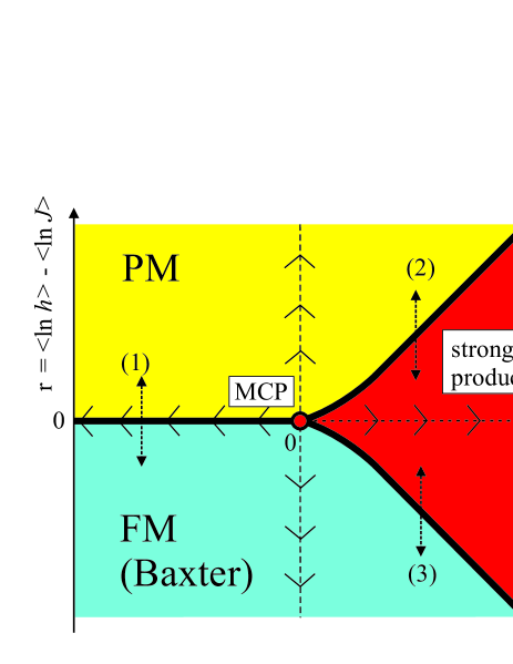
Figure 1: Schematic ground state phase diagram of the two-color random quantum Ashkin-Teller chain. For $\epsilon_{I}<\epsilon_{c}(1)=1$, the paramagnetic and ferromagnetic phases are connected by a direct continuous quantum phase transition. For $\epsilon_{I}>1$, they are separated by a partially ordered “product” phase characterized by strong randomness and renormalization group flow towards infinite coupling. The two regimes are separated by a multicritical point (MCP) at $\epsilon=1$. (after Ref. Hrahsheh et al. (2014)).

For example, the transitions between the product phase and the paramagnetic and ferromagnetic phases (transitions 2 and 3 in Fig. 1) are both of infinite-randomness type and in the random transverse-field Ising universality class.

The strong-coupling behavior of the random quantum Ashkin-Teller chains with $N=3$ and 4 colors could not be worked out with the above methods.

IV.2 Variable transformation for $N=3$

In this and the following subsections, we present a method that allows us to study the strong-coupling regime of the random quantum Ashkin-Teller model for any number $N$ of colors. It is based on a generalization of the variable transformation (9), (10) of the two-color problem. We start by discussing $N=3$ colors which is particularly interesting because it is not covered by the existing work Hrahsheh et al. (2012, 2014). Furthermore, it is the lowest number of colors for which the clean system features a first-order transition. After $N=3$, we consider general odd and even color numbers $N$ which require slightly different implementations.

In the three-color case, the transformation is defined by introducing two pair variables and one product of all three original colors,

$$\sigma_{i}^{z}=S_{1,i}^{z}\,S_{3,i}^{z},\quad\tau_{i}^{z}=S_{2,i}^{z}\,S_{3,i}^{z},\quad\eta_{i}^{z}=S_{1,i}^{z}\,S_{2,i}^{z}\,S_{3,i}^{z}~{}.$$ (12)

The corresponding transformation of the Pauli matrices $S_{\alpha,i}^{x}$ is given by

$$S_{1,i}^{x}=\sigma_{i}^{x}\,\eta_{i}^{x},\quad S_{2,i}^{x}=\tau_{i}^{x}\,\eta_{i}^{x},\quad S_{3,i}^{x}=\sigma_{i}^{x}\,\tau_{i}^{x}\,\eta_{i}^{x}~{}.$$ (13)

Inserting these transformations into the Hamiltonian (II) yields

$$H= -\sum_{i}g_{i}\left(\sigma_{i}^{x}+\tau_{i}^{x}+\sigma_{i}^{x}\tau_{i}^{x}\right)$$

$$-\sum_{i}K_{i}\left(\sigma_{i}^{z}\sigma_{i+1}^{z}+\tau_{i}^{z}\tau_{i+1}^{z}+\sigma_{i}^{z}\sigma_{i+1}^{z}\tau_{i}^{z}\tau_{i+1}^{z}\right)$$

$$-\sum_{i}h_{i}\left(\sigma_{i}^{x}+\tau_{i}^{x}+\sigma_{i}^{x}\tau_{i}^{x}\right)\eta_{i}^{x}$$

$$-\sum_{i}J_{i}\left(\sigma_{i}^{z}\sigma_{i+1}^{z}+\tau_{i}^{z}\tau_{i+1}^{z}+\sigma_{i}^{z}\sigma_{i+1}^{z}\tau_{i}^{z}\tau_{i+1}^{z}\right)\eta_{i}^{z}\eta_{i+1}^{z}.$$

We see that the triple product $\eta_{i}$ does not show up in the terms containing $g_{i}$ and $K_{i}$. In the strong-coupling limit, $\epsilon\gg 1$, $g_{i}$ and $K_{i}$ are much larger than $h_{i}$ and $J_{i}$. The behavior of the pair variables $\sigma_{i}$ and $\tau_{i}$ is thus governed by the first two lines of (IV.2) only and becomes independent of the triple products $\eta_{i}$. The $\eta_{i}$ themselves are slaved to the behavior of the $\sigma_{i}$ and $\tau_{i}$ via the large brackets in the third and fourth line of (IV.2).

The qualitative features of the strong-coupling regime follow directly from these observations. The first two lines of (IV.2) form a two-color random quantum Ashkin-Teller model for the variables $\sigma_{i}$ and $\tau_{i}$. As all terms in the brackets have the same prefactor, this two-color Ashkin-Teller model is right at its multicritical coupling strength $\epsilon_{c}$ (as demonstrated in Ref. Hrahsheh et al. (2014) and shown in Fig. 1). The $\sigma_{i}$ and $\tau_{i}$ thus undergo a direct phase transition between a paramagnetic phase for $g_{\rm typ}>K_{\rm typ}$ and a ferromagnetic phase for $g_{\rm typ}<K_{\rm typ}$. In agreement with the quantum Aizenman-Wehr theorem, the transition is continuous; it is in the infinite-randomness universality class of the random transverse-field Ising model. Moreover, in contrast to the $N=2$ case, there is no additional partially ordered phase.

What about the triple product variables $\eta_{i}$? For large disorder, the brackets in the third and fourth line of (IV.2) can be treated as classical variables. If the $\sigma_{i}$ and $\tau_{i}$ order ferromagnetically, $\sigma_{i}^{x}+\tau_{i}^{x}+\sigma_{i}^{x}\tau_{i}^{x}$ vanishes (for all sites surviving the strong-disorder renormalization group at low energies) while in the paramagnetic phase, $\sigma_{i}^{z}\sigma_{i+1}^{z}+\tau_{i}^{z}\tau_{i+1}^{z}+\sigma_{i}^{z}\sigma_{i+1}^{z}\tau_{i}^{z}\tau_{i+1}^{z}$ vanishes. Thus, each $\eta_{i}$ becomes a classical variable that is slaved to the behavior of $\sigma_{i}$ and $\tau_{i}$. This means, the $\eta_{i}$ align ferromagnetically if the $\sigma_{i}$ and $\tau_{i}$ are ferromagnetic while they form a spin-polarized paramagnet if $\sigma_{i}$ and $\tau_{i}$ are in the paramagnetic phase.

All these qualitative results are confirmed by a strong-disorder renormalization group calculation which we now develop for the case of general odd $N$.

IV.3 Variable transformation and strong-disorder renormalization group for general odd $N$

For general odd $N>2$, we define $N-1$ pair variables and one product of all colors

$$\sigma_{\alpha,i}^{z}=S_{\alpha,i}^{z}\,S_{N,i}^{z}\quad(\alpha=1\ldots N-1),\quad\eta_{i}^{z}=\prod_{\alpha=1}^{N}S_{\alpha,i}^{z}~{}.$$ (15)

The corresponding transformation of the Pauli matrices $S_{\alpha,i}^{x}$ is given by

$$S_{\alpha,i}^{x}=\sigma_{\alpha,i}^{x}\,\eta_{i}^{x}\quad(\alpha=1\ldots N-1),\quad S_{N,i}^{x}=\prod_{\alpha=1}^{N-1}\sigma_{\alpha,i}^{x}\,\eta_{i}^{x}~{}.$$ (16)

In terms of these variables, the Hamiltonian (II) reads

$$H= -\sum_{i}g_{i}{\left[\sum_{\alpha<\beta}^{N-1}\sigma_{\alpha,i}^{x}\sigma_{\beta,i}^{x}+\sum_{\alpha=1}^{N-1}\prod_{k\neq\alpha}^{N-1}\sigma_{k,i}^{x}\right]}$$

$$-\sum_{i}K_{i}{\left[\sum_{\alpha<\beta}^{N-1}\sigma_{\alpha,i}^{z}\sigma_{\alpha,i+1}^{z}\sigma_{\beta,i}^{z}\sigma_{\beta,i+1}^{z}+\sum_{\alpha=1}^{N-1}\sigma_{\alpha,i}^{z}\sigma_{\alpha,i+1}^{z}\right]}$$

$$-\sum_{i}~{}h_{i}{\left[\sum_{\alpha=1}^{N-1}\sigma_{\alpha,i}^{x}+\prod_{k=1}^{N-1}\sigma_{k,i}^{x}\right]}\eta_{i}^{x}$$

$$-\sum_{i}~{}J_{i}{\left[\sum_{\alpha=1}^{N-1}\prod_{k\neq\alpha}^{N-1}\sigma_{k,i}^{z}\sigma_{k,i+1}^{z}+\prod_{k=1}^{N-1}\sigma_{k,i}^{z}\sigma_{k,i+1}^{z}\right]}\eta_{i}^{z}\eta_{i+1}^{z}.$$

As in the three-color case, the $N$-product variable $\eta_{i}$ does not appear in the terms containing the large energies $g_{i}$ and $K_{i}$.

We now implement a strong-disorder renormalization group for the Hamiltonian (IV.3). This can be conveniently done using the projection method described, e.g., by Auerbach Auerbach (1998) and applied to the random quantum Ashkin-Teller model in Ref. Hrahsheh et al. (2014). Within this technique, the (local) Hilbert space is divided into low-energy and high-energy subspaces. Any state $\psi$ can be decomposed as $\psi=\psi_{1}+\psi_{2}$ with $\psi_{1}$ in the low-energy subspace and $\psi_{2}$ in the high-energy subspace. The Schroedinger equation can then be written in matrix form

$$\left(\begin{matrix}H_{11}&H_{12}\\ H_{21}&H_{22}\end{matrix}\right)\left(\begin{matrix}\psi_{1}\\ \psi_{2}\end{matrix}\right)=E\left(\begin{matrix}\psi_{1}\\ \psi_{2}\end{matrix}\right)$$ (18)

with $H_{ij}=P_{i}HP_{j}$. Here, $P_{1}$ and $P_{2}$ project on the low-energy and high-energy subspaces, respectively. Eliminating $\psi_{2}$ from these two coupled equations gives $H_{11}\psi_{1}+H_{12}(E-H_{22})^{-1}H_{21}\psi_{1}=E\psi_{1}$. Thus, the effective Hamiltonian in the low-energy Hilbert space is

$$H_{\rm eff}=H_{11}+H_{12}(E-H_{22})^{-1}H_{21}~{}.$$ (19)

The second term can now be expanded in inverse powers of the large local energy scale $g_{i}$ or $K_{i}$.

In the strong-coupling regime, $\epsilon\gg 1$, the strong-disorder renormalization group is controlled by the first two lines of (IV.3). It does not depend on the $N$-products $\eta_{i}$ which are slaved to the $\sigma_{i}$ and $\tau_{i}$ via the large brackets in the third and forth lines of (IV.3).

If the largest local energy scale is the “Ashkin-Teller field” $g_{i}$, site $i$ does not contribute to the order parameter and is integrated out via a site decimation. The recursions resulting from (19) take the same form as in the weak-coupling regime, i.e., the effective interactions and coupling strength are given by eqs. (2) to (4) .

What about the product variable $\eta_{i}$? The bracket in the third line of the Hamiltonian (IV.3) takes the value $N$ while the bracket in the fourth line vanishes. However, because $h_{i}\ll g_{i}$, the value of $\eta_{i}^{x}$ is not fixed by the renormalization group step. Thus $\tilde{\zeta}_{i}\equiv\eta_{i}^{x}$ becomes a classical Ising degree of freedom with energy $-Nh_{i}\tilde{\zeta}_{i}$ that is independent of the terms in the renormalized Hamiltonian. This means, it is “left behind” in the renormalization group step. Consequently, $\eta_{i}^{x}$ plays the role of the additional “internal degree of freedom” first identified in Ref. Hrahsheh et al. (2012).

The bond decimation step performed if the largest local energy is the four-spin interaction $K_{i}$ can be derived analogously. The recursion relations are again identical to the weak-coupling regime, i.e., the resulting effective field and coupling are given by eqs. (5) to (7). In this step, the bracket in the fourth line of the Hamiltonian (IV.3) takes the value $N$ while the bracket in the third line vanishes. Thus, the renormalization group step leaves behind the classical Ising degree of freedom $\tilde{\zeta}_{i}\equiv\eta_{i}^{z}\eta_{i+1}^{z}$ with energy $-NJ_{i}\tilde{\zeta}_{i}$. In the bond decimation step, the additional “internal degree of freedom” of Ref. Hrahsheh et al. (2012) is thus given by $\tilde{\zeta}_{i}\equiv\eta_{i}^{z}\eta_{i+1}^{z}$.

All of these renormalization group recursions agree with those of Ref. Hrahsheh et al. (2012) where the renormalization group was implemented in the original variables for $N>4$ colors.

IV.4 Variable transformation and strong-disorder renormalization group for general even $N$

For general even $N\geq 4$, the variable transformation is slightly more complicated than in the odd $N$ case. We define $N-2$ pair variables, a product of $N-1$ colors and a product of all $N$ colors,

$$\sigma_{\alpha,i}^{z} = S_{\alpha,i}^{z}\,S_{N-1,i}^{z}\quad(\alpha=1\ldots N-2),$$

$$\eta_{i}^{z}~{} = \prod_{\alpha=1}^{N-1}S_{\alpha,i}^{z}~{},\quad\tau_{i}^{z}=\prod_{\alpha=1}^{N}S_{\alpha,i}^{z}.$$ (20)

The Pauli matrices $S_{\alpha,i}^{x}$ then transform via

$$S_{\alpha,i}^{x}=\sigma_{\alpha,i}^{x}\,\eta_{i}^{x}\,\tau_{i}^{x}\quad(\alpha=1\ldots N-2),$$

$$S_{N-1,i}^{x}=\prod_{\alpha=1}^{N-2}\sigma_{\alpha,i}^{x}\,\eta_{i}^{x}\tau_{i}^{x}~{},\quad S_{N,i}^{x}=\tau_{i}^{x}~{}.$$ (21)

After applying these transformations to the Hamiltonian (II), we obtain

$$H = -\sum_{i=1}^{\infty}g_{i}\left[\sum_{\alpha<\beta}^{N-2}\sigma_{\alpha,i}^{x}\sigma_{\beta,i}^{x}+\sum_{\alpha=1}^{N-2}\prod_{\beta\neq\alpha}^{N-2}\sigma_{\beta,i}^{x}+\right.$$

$$\hskip 99.58464pt+\left.\left(\sum_{\alpha=1}^{N-2}\sigma_{\alpha,i}^{x}+\prod_{\beta=1}^{N-2}\sigma_{\beta,i}^{x}\right)\eta_{i}^{x}\right]$$

$$-\sum_{i=1}^{\infty}K_{i}\left[\sum_{\alpha<\beta}^{N-2}\sigma_{\alpha,i}^{z}\sigma_{\alpha,i+1}^{z}\sigma_{\beta,i}^{z}\sigma_{\beta,i+1}^{z}+\sum_{\alpha=1}^{N-2}\sigma_{\alpha,i}^{z}\sigma_{\alpha,i+1}^{z}+\right.$$

$$\hskip 14.22636pt+\left.\left(\sum_{\alpha=1}^{N-2}\prod_{\beta\neq\alpha}^{N-2}\sigma_{\beta,i}^{z}\sigma_{\beta,i+1}^{z}+\prod_{\beta=1}^{N-2}\sigma_{\beta,i}^{z}\sigma_{\beta,i+1}^{z}\right)\tau_{i}^{z}\tau_{i+1}^{z}\right]$$

$$-\sum_{i=1}^{\infty}~{}h_{i}\left[\left(\sum_{\alpha=1}^{N-2}\sigma_{\alpha,i}^{x}\eta_{i}^{x}+\prod_{\beta=1}^{N-2}\sigma_{\beta,i}^{x}\eta_{i}^{x}\right)+1\right]\tau_{i}^{x}$$

$$-\sum_{i=1}^{\infty}~{}J_{i}\left[\sum_{\alpha=1}^{N-2}\prod_{\beta\neq\alpha}^{N-2}\sigma_{\beta,i}^{z}\sigma_{\beta,i+1}^{z}+\prod_{\beta=1}^{N-2}\sigma_{\beta,i}^{z}\sigma_{\beta,i+1}^{z}+\right.$$

$$\hskip 156.49014pt+\tau_{i}^{z}\tau_{i+1}^{z}{\Bigg{]}}\eta_{i}^{z}\eta_{i+1}^{z}.$$

In contrast to the odd $N$ case, the decoupling between the pair variables $\sigma_{\alpha,i}$ and the $(N-1)$ and $N$-products $\eta_{i}$ and $\tau_{i}$ is not complete. Each of the products is contained in one but not both of the terms that dominate for strong coupling $\epsilon\gg 1$ (first two lines of (IV.4)). As a result, the phase diagram in the strong-coupling regime is controlled by a competition between the $\sigma_{\alpha,i}^{z}$ and $\sigma_{\alpha,i}^{x}$ via the first two lines of (IV.4) while the $\eta_{i}$ and $\tau_{i}$ variables are slaved to them. It features a direct transition between the ferromagnetic and paramagnetic phases at $g_{\rm typ}=K_{\rm typ}$, in agreement with the self-duality of the original Hamiltonian.

To substantiate these qualitative arguments, we have implemented the strong-disorder renormalization group for the Hamiltonian (IV.4), using the projection method as in the last subsection. In the case of a site decimation, i.e., if the largest local energy is the “Ashkin-Teller field” $g_{i}$, we again obtain the recursion relations (2) to (4). The variable $\tau_{i}^{x}$ is not fixed by the renormalization group. Thus $\tilde{\zeta}_{i}\equiv\tau_{i}^{x}$ represents the extra classical Ising degree of freedom that is left behind in the renormalization group step. Its energy is $-Nh_{i}\tilde{\zeta}_{i}$. If the largest local energy is the four-spin interaction $K_{i}$, we perform a bond decimation. The resulting recursions relations agree with the weak-coupling recursions (5) to (7). In this case, the product $\eta_{i}^{z}\eta_{i+1}^{z}$ is not fixed by the decimation step. Therefore, the left-behind Ising degree of freedom in this decimation step is $\tilde{\zeta}_{i}\equiv\eta_{i}^{z}\eta_{i+1}^{z}$ with energy $-NJ_{i}\tilde{\zeta}_{i}$.

The above strong-disorder renormalization group works for all even color numbers $N>4$. For $N=4$, an extra complication arises because the left-behind internal degrees of freedom $\tilde{\zeta}_{i}$ do not decouple from the rest of the Hamiltonian. For example, when decimating site $i$ (because $g_{i}$ is the largest local energy), the $\tau^{z}$ term in the fourth line of (IV.4) mixes the two states of the left-behind $\tau_{i}^{x}$ degree of freedom in second order perturbation theory. An analogous problem arises in a bond decimation step. Thus, for $N=4$ colors, the internal $\tilde{\zeta}_{i}$ degrees of freedom need to be kept, and the renormalization group breaks down. In contrast, for $N>4$, the coupling between the internal $\tilde{\zeta}_{i}$ degrees of freedom and the rest of the Hamiltonian only appears in higher order of perturbation theory and is thus renormalization-group irrelevant.

IV.5 Renormalization group flow, phase diagram, and observables

For color numbers $N=3$ and all $N>4$, the strong-disorder renormalization group implementations of the last two subsections all lead to the recursion relations (2) to (7). The behavior of these recursions has been studied in detail in Ref. Hrahsheh et al. (2012). In the following, we therefore summarize the resulting renormalization group flow, phase diagram, and key observables.

According to (4) and (7), the coupling strengths $\epsilon$ flow to infinity if their initial value $\epsilon_{I}>\epsilon_{c}(N)$. Moreover, the competition between interactions $K_{i}$ and “fields” $g_{i}$ is governed by the recursion relations (3) and (6) which simplify to

$$\tilde{K}=\frac{K_{i-1}K_{i}}{2(N-2)g_{i}}~{},\quad\tilde{g}=\frac{g_{i}g_{i+1}}{2(N-2)K_{i}}$$ (23)

in the large-$\epsilon$ limit. They take the same form as Fisher’s recursions of the random transverse-field Ising model Fisher (1995). (The extra constant prefactor $2(N-2)$ is renormalization-group irrelevant). The renormalization group therefore leads to a direct continuous phase transition between the ferromagnetic and spin-polarized paramagnetic phases on the self-duality line $g_{\rm typ}=K_{\rm typ}$ (or, equivalently, $h_{\rm typ}=J_{\rm typ}$) . The renormalization group flow on this line is sketched in Fig. 2.

Figure 2: Schematic of the renormalization-group flow diagram on the self-duality line of the random quantum Ashkin-Teller model with $N=3$ or $N>4$ colors in the disorder–coupling strength parameter space. For $\epsilon<\epsilon_{c}(N)$ (left arrows), the critical flow approaches the usual Ising infinite-randomness critical point of Ref. Fisher, 1995. For $\epsilon>\epsilon_{c}$ (right arrows), we find a distinct infinite-randomness critical point with even stronger thermodynamic singularities (after Ref. Hrahsheh et al. (2012)).

In the weak-coupling regime, $\epsilon_{I}<\epsilon_{c}(N)$, the flow is towards the random-transverse field Ising quantum critical point located at infinite disorder and $\epsilon=0$, as explained in Sec. III. In the strong-coupling regime, $\epsilon_{I}>\epsilon_{c}(N)$, the $N$-color random quantum Ashkin-Teller model ($N=3$ and $N>4$) features a distinct infinite-randomness critical fixed point at infinite disorder and infinite coupling strength. It is accompanied by two lines of fixed points for $r=\ln(g_{\rm typ}/K_{\rm typ})>0$ ($r<0$) that represent the paramagnetic (ferromagnetic) quantum Griffiths phases.

The behavior of thermodynamic observables in the strong-coupling regime at criticality and in the Griffiths phases can be worked out by incorporating the left-behind internal degrees of freedom $\zeta$ in the renormalization-group calculation. This divides the renormalization group flow into two stages and leads to two distinct contributions to the observables Hrahsheh et al. (2012). For example, the temperature dependence of the entropy at criticality takes the form

$$S=C_{1}\left[\ln{\left(\frac{\Omega_{I}}{T}\right)}\right]^{-\frac{1}{\psi\phi}}\ln 2+C_{2}\left[\ln{\left(\frac{\Omega_{I}}{T}\right)}\right]^{-\frac{1}{\psi}}N\ln 2,$$ (24)

where $\psi=1/2$ is the tunneling exponent, $\phi=\frac{1}{2}(1+\sqrt{5})$, $C_{1}$ and $C_{2}$ are nonuniversal constants, and $\Omega_{I}$ is the bare energy cutoff. The second term is the usual contribution of clusters surviving under the strong-disorder renormalization group to energy scale $\Omega=T$. The first term represents all internal degrees of freedom $\zeta$ left behind until the renormalization group reaches this scale. As $\phi>1$, the low-$T$ entropy becomes dominated by the extra degrees of freedom $S\to S_{\rm extra}\sim[\ln(\Omega_{I}/T)]^{-1/(\phi\psi)}$. Analogously, in the Griffiths phases, the contribution of the internal degrees of freedom gives

$$S_{\rm extra}\sim|r|^{\nu}(T/\Omega_{I})^{1/(z+Az^{\phi})}\ln 2,$$ (25)

which dominates over the regular chain contribution proportional to $T^{1/z}N\ln 2$. Here, $\nu=2$ is the correlation length critical exponent, and $z=1/(2|r|)$ is the non-universal Griffiths dynamical exponent. Other observables can be calculated along the same lines Hrahsheh et al. (2012).

The weak and strong coupling regimes are separated by a multicritical point located at $r=0$ and $\epsilon_{I}=\epsilon_{c}(N)$. At this point, the renormalization group flow has two unstable directions, $r=\ln(g_{\rm typ}/K_{\rm typ})$ and $\epsilon_{I}-\epsilon_{c}(N)$. The flow in $r$ direction can be understood by inserting $\epsilon_{c}(N)$ into the recursion relations (2) and (5) yielding

$$\tilde{J}=\frac{J_{i-1}J_{i}}{(1+(N-1)\epsilon_{c})h_{i}}~{},\quad\tilde{h}=\frac{h_{i}h_{i+1}}{(1+(N-1)\epsilon_{c})J_{i}}~{}.$$ (26)

These recursions are again of Fisher’s random transverse-field Ising type (as the prefactor $(1+(N-1)\epsilon_{c})$ is renormalization-roup irrelevant). Thus, the renormalization group flow at the multicritical point agrees with that of the weak-coupling regime. Note, however, that the $N$ transverse-field Ising chains making up the Ashkin-Teller model do not decouple at the multicritical point. Thus, the fixed-point Hamiltonians of the weak-coupling fixed point and the multicritical point do not agree.

The flow in the $\epsilon$ direction can be worked out by expanding the recursions (4) and (7) about the fixed point value $\epsilon_{c}(N)$ by introducing $\delta_{J,i}=\epsilon_{J,i}-\epsilon_{c}$ and $\delta_{h,i}=\epsilon_{h,i}-\epsilon_{c}$. This leads to the recursions

$$\tilde{\delta}_{J}=\delta_{J,i}+\delta_{J,i+1}+Y\delta_{h_{i}}~{},\quad\tilde{\delta}_{h}=\delta_{h,i}+\delta_{h,i+1}+Y\delta_{J,i}$$ (27)

with $Y=\epsilon_{c}/[(1+(N-1)\epsilon_{c})(1+(N-2)\epsilon_{c})]$. Recursions of this type have been studied in detail by Fisher in the context of antiferromagnetic Heisenberg chains Fisher (1994) and the random transverse-field Ising chain Fisher (1995). Using these results, we therefore find that $\delta$ scales as

$$\delta_{\rm typ}(\Gamma)\approx\Gamma^{\phi_{Y}}\,\delta_{I},\qquad\phi_{Y}=\frac{1}{2}(1+\sqrt{5+4Y})$$ (28)

with the renormalization group energy scale $\Gamma=\ln(\Omega_{I}/\Omega)$. The crossover from the multicritical scaling to either the weak-coupling or the strong-coupling fixed point occurs when $|\delta_{\rm typ}|$ reaches a constant $\delta_{x}$ of order unity. It thus occurs at an energy scale $\Gamma_{x}=|\delta_{x}/\delta_{I}|^{1/\phi_{Y}}$.

V Conclusions

To summarize, we have investigated the ground state phase diagram and quantum phase transitions of the $N$-color random quantum Ashkin-Teller chain which is one of the prototypical models for the study of various strong-disorder effects at quantum phase transitions. After reviewing existing strong-disorder renormalization group approaches, we have introduced a general variable transformation that allows us to treat the strong-coupling regime for $N>2$ in a unified fashion.

For all color numbers $N>2$, we find a direct transition between the ferromagnetic and paramagnetic phases for all (bare) coupling strengths $\epsilon_{I}\geq 0$. Thus, an equivalent of the partially ordered product phase in the two-color model does not exist for three or more colors. In agreement with the quantum version of the Aizenman-Wehr theorem Greenblatt et al. (2009), this transition is continuous even if the corresponding transition in the clean problem is of first order. Moreover, the transition is of infinite-randomness type, as predicted by the classification of rare regions effects put forward in Refs. Vojta and Schmalian (2005); Vojta (2006) and recently refined in Refs. Vojta and Hoyos (2014); Vojta et al. (2014). Its critical behavior depends on the coupling strength. In the weak-coupling regime $\epsilon<\epsilon_{c}(N)$, the critical point is in the random transverse-field Ising universality class because the $N$ Ising chains that make up the Ashkin-Teller model decouple in the low-energy limit. In the strong-coupling regime, $\epsilon>\epsilon_{c}(N)$, we find a distinct infinite-randomness critical point that features even stronger thermodynamic singularities stemming from the “left-behind” internal degrees of freedom.

The novel variable transformation also allowed us to study the multicritical point separating the weak-coupling and strong-coupling regimes. Its renormalization-group flow has two unstable directions. The flow for $r=\ln(g_{\rm typ}/K_{\rm typ})\neq 0$ and $\epsilon_{I}-\epsilon_{c}(N)=0$ is identical to the flow in the weak-coupling regime implying identical critical exponents. The flow at $r=0$ in the $\epsilon$ direction is controlled by different recursions for $\delta=\epsilon-\epsilon_{c}(N)$ which we have solved for general $N$.

So far, we have focused on systems whose (bare) coupling strengths are uniform $\epsilon_{J,i}=\epsilon_{h,i}=\epsilon_{I}$. What about random coupling strengths? If all $\epsilon_{J,i}$ and $\epsilon_{h,i}$ are smaller than the multicritical value $\epsilon_{c}(N)$, the renormalized $\tilde{\epsilon}$ decrease under the renormalization group just as in the case of uniform bare $\epsilon$. If, on the other hand, all $\epsilon_{J,i}$ and $\epsilon_{h,i}$ are above $\epsilon_{c}(N)$, the renormalized values $\tilde{\epsilon}$ increase under renormalization as in the case of uniform bare $\epsilon$. Therefore, our qualitative results do not change; in particular, the bulk phases are stable against weak randomness in $\epsilon$. The same holds for the transitions between the ferromagnetic and paramagnetic phases sufficiently far away from the multicritical point. Note that this also explains why the randomness in $\epsilon$ produced in the course of the strong-disorder renormalization group is irrelevant if the initial (bare) $\epsilon$ are uniform: All renormalized $\epsilon$ values are on the same side of the multicritical point and thus flow either to zero or to infinity.

In contrast, the uniform-$\epsilon$ multicritical point itself is unstable against randomness in $\epsilon$. The properties of the resulting random-$\epsilon$ multicritical point can be studied numerically in analogy to the two-color case Hrahsheh et al. (2014). This remains a task for the future.

References

- Onsager (1944) L. Onsager, Phys. Rev. 65, 117 (1944).
- Sachdev (1999) S. Sachdev, Quantum phase transitions (Cambridge University Press, Cambridge, 1999).
- Ashkin and Teller (1943) J. Ashkin and E. Teller, Phys. Rev. 64, 178 (1943).
- Kohmoto et al. (1981) M. Kohmoto, M. den Nijs, and L. P. Kadanoff, Phys. Rev. B 24, 5229 (1981).
- Igloi and Solyom (1984) F. Igloi and J. Solyom, J. Phys. A 17, 1531 (1984).
- Grest and Widom (1981) G. S. Grest and M. Widom, Phys. Rev. B 24, 6508 (1981).
- Fradkin (1984) E. Fradkin, Phys. Rev. Lett. 53, 1967 (1984).
- Shankar (1985) R. Shankar, Phys. Rev. Lett. 55, 453 (1985).
- Vojta (2006) T. Vojta, J. Phys. A 39, R143 (2006).
- Vojta (2010) T. Vojta, J. Low Temp. Phys. 161, 299 (2010).
- Harris (1974) A. B. Harris, J. Phys. C 7, 1671 (1974).
- Aizenman and Wehr (1989) M. Aizenman and J. Wehr, Phys. Rev. Lett. 62, 2503 (1989).
- Greenblatt et al. (2009) R. L. Greenblatt, M. Aizenman, and J. L. Lebowitz, Phys. Rev. Lett. 103, 197201 (2009).
- Bak et al. (1985) P. Bak, P. Kleban, W. N. Unertl, J. Ochab, G. Akinci, N. C. Bartelt, and T. L. Einstein, Phys. Rev. Lett. 54, 1539 (1985).
- Aji and Varma (2007) V. Aji and C. M. Varma, Phys. Rev. Lett. 99, 067003 (2007).
- Aji and Varma (2009) V. Aji and C. M. Varma, Phys. Rev. B 79, 184501 (2009).
- Chang et al. (2008) Z. Chang, P. Wang, and Y.-H. Zheng, Commun. Theor. Phys. 49, 525 (2008).
- Baxter (1982) R. Baxter, Exactly Solved Models in Statistical Mechanics (Academic Press, New York, 1982).
- Dotsenko (1985) V. S. Dotsenko, J. Phys. A 18, L241 (1985).
- Giamarchi and Schulz (1988) T. Giamarchi and H. J. Schulz, Phys. Rev. B 37, 325 (1988).
- Goswami et al. (2008) P. Goswami, D. Schwab, and S. Chakravarty, Phys. Rev. Lett. 100, 015703 (2008).
- Carlon et al. (2001) E. Carlon, P. Lajkó, and F. Iglói, Phys. Rev. Lett. 87, 277201 (2001).
- Fisher (1992) D. S. Fisher, Phys. Rev. Lett. 69, 534 (1992).
- Fisher (1995) D. S. Fisher, Phys. Rev. B 51, 6411 (1995).
- Hrahsheh et al. (2012) F. Hrahsheh, J. A. Hoyos, and T. Vojta, Phys. Rev. B 86, 214204 (2012).
- Hrahsheh et al. (2014) F. Hrahsheh, J. A. Hoyos, R. Narayanan, and T. Vojta, Phys. Rev. B 89, 014401 (2014).
- Auerbach (1998) A. Auerbach, Interacting Electrons and Quantum Magnetism (Springer, New York, 1998).
- Note (1) Strictly, (2) to (4) hold in the ground-state sector, while in the pseudo ground state, , the transverse field shows up with the opposite sign. This difference is irrelevant close to the fixed point because diverges (see Sec. IV.5). Analogous statements also holds for bond decimations and for even .
- Fisher (1994) D. S. Fisher, Phys. Rev. B 50, 3799 (1994).
- Vojta and Schmalian (2005) T. Vojta and J. Schmalian, Phys. Rev. B 72, 045438 (2005).
- Vojta and Hoyos (2014) T. Vojta and J. A. Hoyos, Phys. Rev. Lett. 112, 075702 (2014).
- Vojta et al. (2014) T. Vojta, J. Igo, and J. A. Hoyos, Phys. Rev. E 90, 012139 (2014).