TARDIS: Stably shifting traffic in space and time

Abstract

This paper describes TARDIS (Traffic Assignment and Retiming Dynamics with Inherent Stability) which is an algorithmic procedure designed to reallocate traffic within Internet Service Provider (ISP) networks. Recent work has investigated the idea of shifting traffic in time (from peak to off-peak) or in space (by using different links). This work gives a unified scheme for both time and space shifting to reduce costs. Particular attention is given to the commonly used 95th percentile pricing scheme.

The work has three main innovations: firstly, introducing the Shapley Gradient, a way of comparing traffic pricing between different links at different times of day; secondly, a unified way of reallocating traffic in time and/or in space; thirdly, a continuous approximation to this system is proved to be stable. A trace-driven investigation using data from two service providers shows that the algorithm can create large savings in transit costs even when only small proportions of the traffic can be shifted.

1 Introduction

Internet Service Providers (ISPs) that are predominantly used by residential users (sometimes called eyeball ISPs) typically have traffic patterns which are dominated by incoming traffic as their typical user downloads more than they upload. Managing this traffic to reduce cost, network congestion and network instability is a primary concern of such network operators. Traditionally, networks have attempted to manage demand through a combination of traffic shaping, artificially curbing demand, and traffic engineering through routing optimisations. Some recent research has considered alternative solutions, moving the incoming traffic in space (by downloading content from different physical locations) [20, 4, 6] or in time (by shifting delay-tolerant traffic to the off-peak) [12, 10, 9]. Both temporal and spatial traffic shifting share the same underlying premise: that reallocating traffic can improve network performance (by reducing costs, increasing stability or other goals). This work all deals with redistributing the traffic into and out of an ISPs network. However, usually the assumptions are simply to move the traffic to a “cheaper link" or to the “off peak". In fact the trade offs may not be so simple and moving too much traffic may worsen the situation. This paper presents a procedure for pricing the times and locations and an algorithm which shows how this price can be used to redistribute traffic in a stable way. A continuous time approximation of the algorithm is provably stable.

Spatial shifting of traffic is studied in a number of contexts. It is often the case that content can be downloaded from different physical locations. In some hosting infrastructures as much as 93% of content is hosted in multiple locations and by one estimate 40% of traffic could be downloaded from three or more locations [1]. Systems in common use which replicate content across locations include peer-to-peer (P2P) systems, content distribution networks (CDNs) and one-click hosting services (OCH). In these systems a number of methods have been proposed or demonstrated which show that these extra copies can be exploited to reduce traffic costs or for other engineering goals [20, 4, 6]. Even when content is available from only a single source then spatial shifting of traffic is possible by using alternative routes [7] in a multi-homed network.

In parallel, multiple papers have explored the potential for shifting delay-tolerant traffic to off-peak hours. In [12] the authors describe a mechanism that offers users higher bandwidth off-peak if they deliberately delay some of their traffic. Further contributions [10, 9, 3] represent similar attempts to shift traffic in time through user incentive schemes.

The papers above (and others) present a number of different alternative means to move traffic in either space and time and it seems certain more will arise in other contexts (for example, content centric networking explicitly encourages content to be available from multiple sources). This paper presents a control algorithm which could be used with any of the above systems alone or in parallel. The goal presented in this paper is traffic cost reduction but other engineering aims could be brought in as well for example avoiding the onset of congestion on a link.

The contributions of this paper are threefold. Firstly, the Shapley gradient is introduced, a means to compare the costs associated with traffic flows from different sources at different times and subject to different pricing schemes. This is a general mechanism which, while focused on the 95th percentile common in transit pricing, can be used for many cost models common for ISPs. Secondly, a unified mathematical framework is presented for reallocating traffic across both time and space. The algorithm shows how traffic allocation should respond to prices by shifting traffic. Thirdly this reallocation strategy is shown to be stable. The dynamical system representation of this mechanism is shown to converge to a beneficial state for the system under weak conditions. The properties of TARDIS are verified through analysis of real traffic traces from a large European ISP and a Japanese academic network.

The structure of the paper is as follows. Section 2 gives background and related work in the area. Section 4 describes an algorithm which can translate groups of links and pricing schemes to comparable costs for putting traffic on the network from a given source at a given time. Section 5 creates a dynamical systems model of the traffic shifting in response to the calculated costs. Section 6 describes a software model of the system and section 7 gives an evaluation using real user traffic data. Finally section 8 gives conclusions about the TARDIS system.

1.1 A brief description of the TARDIS procedure

This section briefly describes the TARDIS procedure as a whole. The focus of the procedure is to control where and when traffic should be assigned as it arrives on a network. If a requested download could be made from a different location or if it could be shifted in time (by several hours) to the off-peak then the TARDIS procedure calculates at what time and location the traffic should be placed in order to minimise costs. The mechanisms by which this reassignment could occur are dealt with by many other papers in the literature (as detailed in section 2) and several different mechanisms are proposed. The exact details of the mechanism used for reassignment do not affect the TARDIS procedure.

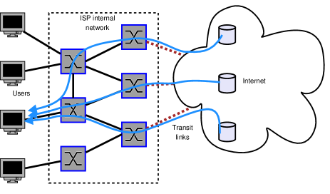
Figure 1: An eyeball ISP network where a user can download requested content from three different transit links.

Figure 1 shows the situation envisaged where shifting in space is possible. In this case, the user wishes to download content which is not available from the ISP’s internal network. The content is available from three separate transit links that are charged at different rates. The decision as to which transit link to use is not trivial as it is not always possible to know which link is “cheapest" at a given time. This is discussed in depth in section 4. Note that, of course, some links may be peering links not transit links, this does not affect TARDIS if the pricing model is one which can be addressed by the TARDIS system. Consideration to these pricing schemes is given in sections 4.3.4 and 4.3.5.

TARDIS is given as input a cost model (details of how the ISP is to be charged for its traffic) and the available choices for a given piece of traffic (the times and locations to which that traffic could be assigned, which of course, includes the possibility it cannot move at all). The TARDIS model then computes splitting rates which describe the desired proportion of traffic from the choice set which should be assigned to each time and location. Note that obviously individual flows are not split up to different destinations and times.

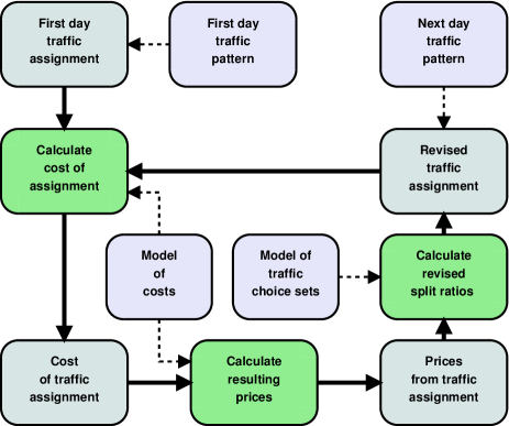
Figure 2: The TARDIS scheme for shifting traffic in space and time to reduce costs.

Figure 2 shows the basic iterative loop which would be used by TARDIS. The dotted lines show input, the solid lines flow of control. On the first day, traffic is assigned without modification. The resulting costs arising from this assignment are calculated from a model of how the ISP is charged for their traffic. These costs are used to calculate virtual prices for traffic which is assigned to a given time and location. The mechanism for this calculation is described in section 4. These prices are used to calculate splitting ratios which could be interpreted as the probabilities of traffic choosing between various destinations (or times) picking a given destination. The mechanism for calculating the splitting ratios is given in section 5. These splitting ratios will, in combination with the traffic placed on the network create a new cost. The new cost will create new prices and so on. Obviously it is of primary importance that this system is stable and this is proved in section 5 for a continuous time approximation of the system.

2 Background

ISPs pay for traffic on their networks in a variety of ways either directly through charges levied based upon the traffic level or indirectly by paying for the cost of leasing appropriate network capacity. In transit networks the most common way to charge for traffic is 95th percentile pricing (see section 4.1). If 95th percentile pricing is applied to traffic generated by many users, it is natural to ask how much each user contributes to the total cost and how this could be mapped to a cost per time period. One answer to this question is given in [17], where the authors use the Shapley value to find user cost contributions and least-squares fitting to find the unit costs that best approximate the Shapley value as a function of the traffic volume and time of day. This is described more fully in section 4.1. In [18] the authors consider pricing strategies for transit ISPs noting that transit traffic prices vary according to destination. They find that the strategy of discounting local traffic is not optimal and instead suggest an automatic way to bundle traffic into a small number of pricing tiers according to cost and demand. In [13] the authors consider the benefits of ISPs changing routing decisions to move traffic around their internal network to reduce cost. They account for a number of different network costs including fixed costs, interconnect costs, transit and backhaul. They produce an optimisation model which outputs routing decisions and uses the Shapley value formulation from [17] to assess traffic where 95th percentile billing is used. The work is considerably different in scope and intent to this paper. Their aim is to produce a comprehensive cost model and demonstrate that routing decisions in the internal network could save costs given a fixed traffic matrix. This paper takes a simpler cost model and focuses on the strategies which could be used to save costs by altering the traffic matrix. In fact, the cost models from [13] could be used as an input to the TARDIS system to improve its ability to shift traffic on the internal network as well as external traffic. The costs models formulated in [13] could all be translated simply to the Shapley gradient formulation in section 4.

A number of authors have investigated how eyeball ISPs can reduce their traffic costs by incentivising users to delay downloads. In [10] and [9], the authors describe a model which uses a control loop to adapt the prices that ISPs charge users in response to changes in their bandwidth consumption. This provides an incentive for users to shift part of their traffic to off-peak times. Another deferred download scheme is the Internet Post Office [12] in which users request files and the ISP downloads them off-peak and temporarily stores them so that users can quickly retrieve the local copies when they next log on. The idea is further developed in [3] which uses real user data to estimate the cost reductions provided by such time delays.

Spatial shifting of external traffic is studied in various contexts. Routing via different transit links in a multi-homed network (to/from the same destination) is studied in [7] which solves the problem of rerouting to reduce network costs either for percentile based pricing or linear cost pricing but not a mixture. In [8] the authors investigate cooperation between content providers and ISPs for traffic engineering and to improve server selection by choosing which replica to download from. Their system shows several benefits from merely information sharing about connections and larger benefits from more active cooperation in choice of physical location for connections.

For peer-to-peer systems a number of systems exist. ALTO/P4P [20] was tested in simulation and experiment and shown to reduce network transit costs. ONO [4] which was deployed and reduced inter ISP traffic by changing peer selection. The ALTO/P4P approach is to introduce an interface between ISPs and overlay applications with the purpose of facilitating the selection of overlay nodes based on locality. In [15] the authors assess the extent to which BitTorrent swarms can be localised, i.e. downloads can be kept within an ISPs own network, reducing the ISPs transit costs. The authors consider various strategies to bias overlay topology construction towards local peers, and develop the concept of inherent localisability, which assesses the download performance of swarms using largely local connections within an ISP. Unfortunately, the degree of localisability depends heavily both on the nature of the torrent and the ISP.

Opportunities for space shifting are also widely recognised within Content Distribution Networks (CDNs), which present both high content replication and transparency in traffic redirection. In [14], for example, alterations are made to DNS servers in order to serve traffic from different CDN hosts transparently to the end user. In [6] the authors propose content aware traffic engineering (CaTE), which allows ISPs to take advantage of content available in multiple locations to reduce link utilisation. The authors show that the gains can be substantial: more than 32% of the traffic in their dataset can be be delivered from at least 8 different subnets, and almost 40% of traffic can be obtained from 3 or more locations. This estimate focuses on traffic from major providers and does not include, for example, P2P.

One-click hosting services could provide another opportunity for spatially shifting traffic as they contribute a large proportion to traffic share and many are multi-homed [2].

The proposed TARDIS algorithm could be used in combination with any of the systems from [14, 6, 20, 4, 10, 9, 13, 12] as a control system to suggest which reallocations would most benefit the ISP.

3 Definitions

Some definitions are made here to simplify further discussion and to gather terms for the rest of the paper.

Define a traffic pricing group (TPG) as traffic grouped together for pricing purposes. In the simplest case this may be traffic over a single physical link. It may also represent several links where the traffic is aggregated to produce a final price or even a subset of traffic on a single link priced differently. The latter arises for example when providers charge for national and international traffic at different rates, a practice often referred to as unbundling [18].

Define a traffic slot as a specific TPG associated with a specific time window. Hence, a set of traffic slots represents a choice of TPGs and time windows to which traffic volumes could be allocated. For example, one set of slots may represent the possibility of downloading from a fixed location at any time in the next eight hours; another may represent the possibility of downloading only during the current time window, but from many different TPGs.

The main variables used in the next sections can be found in the following table.

$v(\mathcal{S})$	Total cost of a TPG for traffic from users in set $\mathcal{S}$
$p_{i}$	price of using slot $i$
$\mathcal{C}_{j}$	Set of slots making up the $j$th choice set
$d_{i}$	Traffic demand in bytes for traffic which could be assigned to any slot in $\mathcal{C}_{i}$
$X_{ij}$	Traffic flow in bytes which could be assigned to any slot in $\mathcal{C}_{i}$ and is assigned to slot $j$
$s_{ij}$	the proportion of traffic which could be assigned to any slot in $\mathcal{C}_{i}$ and is assigned to slot $j$

The following notational conventions are used throughout this paper. Lower case bold (e.g. $\mathbf{x}$) indicates vectors. Calligraphic script indicates sets (e.g. $\mathcal{S})$. Upper case bold indicates a matrix or a vector of sets (e.g. $\mathbf{X}$).

4 Pricing

ISPs typically pay a number of different costs for traffic entering and leaving their network their network. These may include fixed costs such as provisioning a link of fixed capacity on their internal network, or to an Internet eXchange Point (IXP) and variable costs, for example a transit link which is charged according to the volume of traffic used. Of particular importance is the 95th percentile pricing scheme, described in section 4.1. The nature of the 95th percentile pricing scheme makes it difficult to deal with analytically (as will be explained in the next section). In previous work [17] the Shapley value has been used to estimate the price of a particular time and link.

Through this section the words “price" and “cost" will be used with very specific meanings. The cost of a traffic pattern is an outcome of the shape of the traffic and the pricing scheme imposed – it is the monetary value which would actually be paid for that traffic using that scheme. The price will be used in this section to mean a notional marker for a given traffic slot which indicates the likely cost impact of assigning traffic to that slot. This price is used as an internal mechanism to work out which traffic slots should be avoided. If small amounts of traffic are moved from a high price slot to a low price slot then it would be expected that the cost would drop.

The following properties are useful for the price chosen:

1. The price can be quickly calculated.

2. An increase of traffic in a slot never causes the price of that slot to fall (monotonic with traffic).

3. The price is differentiable with respect to traffic.

The first condition is for practicality. The second condition simply says adding traffic never makes the price go down. The second and third conditions are used in the stability proof in section 5.

In this paper the Shapley gradient is introduced to solve this problem. This can be considered to answer the question “what is the likely increase in cost which would be caused by adding traffic to this link?" in a robust way which can account for a wide variety of pricing schemes including, naturally, the 95th percentile.

4.1 95th percentile pricing in brief

For transit traffic, ISPs are commonly charged for the 95th percentile of their traffic. This works as follows. For each TPG the 95th percentile cost is set to some fixed value e.g. $r$ dollars per GBps (note that this is a rate not an absolute value). For the charging period $T$ (a typical value is a month) the traffic is divided into smaller time windows of length $t$ (often 5 minutes is used). For each window $i$ the average traffic rate $f_{i}$ is calculated (it is the total traffic in that window divided by $t$ the window length). Define $f^{(95)}$ to be the traffic rate $f_{i}$ such that only $5\%$ of the $f_{i}$ are larger than $f^{(95)}$. The price charged for the period $T$ is then simply $rf^{(95)}$. It is usual that inbound and outbound traffic are tracked separately, and only the largest charged (see [5]). For eyeball ISPs this will almost always be the inbound traffic as this is larger in volume than the outbound traffic. The 95th percentile pricing provides a particular challenge for any scheme which aims to reassign traffic. In particular the question “how does adding traffic to this slot affect the amount paid?" becomes problematic. Adding or taking away a small amount of traffic to any slot has no affect on the cost unless that slot is one with traffic level $f^{(95)}$ for that TPG. A more subtle analysis is required and this is provided by building on the Shapley value as studied in [17].

4.2 Calculating prices using the Shapley gradient

Consider the traffic in a single TPG with a known pricing scheme and with $N$ users. Let $v(\mathcal{S})$ be the total cost which would be paid using this scheme for the traffic generated by a some set of users $\mathcal{S}$. Define $\mathcal{N}$ as the set of all $N$ users. The Shapley value is a concept from game theory which assesses the contribution of a user’s strategy to an overall cost/benefit. The Shapley value (see [17]) of the $i$th user is defined as

$$\phi_{i}=\frac{1}{N!}\sum_{\pi\in\mathcal{S}_{\mathcal{N}}}[v(\mathcal{S}(\pi,i))-v(\mathcal{S}(\pi,i)\backslash i)]\mbox{,}$$ (1)

where $\mathcal{S}_{\mathcal{N}}$ is the set of all $N!$ possible permutations of $\mathcal{N}$, $\pi$ is one such permutation, and $\mathcal{S}(\pi,i)$ is the set of users who arrive not later than $i$ in the permutation $\pi$. Intuitively, (1) can be interpreted as randomising the order of users, estimating the cost incurred by each user $i$ and averaging this cost over all possible user orderings. In [17] the Shapley value of a user’s traffic is used to assign a cost to each hour of the day which reflects the possibility of traffic in that slot contributing to an increased price. The full calculation of the Shapley value (1) requires considering $N!$ combinations of user traffic to analyse traffic from $N$ users but [17] shows that a relatively small sampling gives an efficient, unbiased estimator (in their work 1,000 orderings produced a low error estimate) and this sampling technique is used here.

In [17] this value (that differs for every user) is combined with a least squares fit to get an average cost to assign to each hour. However, this procedure is computationally intensive (calculating the Shapley value for every user and then doing a least squares fit) and does not produce a cost which can be compared to other pricing schemes. What is required is some measure of the cost of adding a small amount of traffic on a given TPG at a given time. This is achieved by considering the gradient of the Shapley value.

Define the Shapley gradient as the rate of increase in cost when a fictitious user $N+1$ injects an additional small amount of traffic $du$ in slot $j$. The Shapley gradient is therefore,

$$G_{j} =\frac{1}{du\,(N+1)!}$$

$$\sum_{\pi\in\mathcal{S}_{\mathcal{N}^{\prime}}}[v(\mathcal{S}(\pi,N+1))-v(\mathcal{S}(\pi,N+1)\backslash N+1)],$$ (2)

where $\mathcal{S}_{\mathcal{N}^{\prime}}$ is the set of arrangements of the users $\mathcal{N}$ plus the fictitious $(N+1)$th user and $\mathcal{S}(\pi,N+1)$ is the set of all users arriving not later than user $N+1$ in the permutation $\pi$.

Define the Shapley gradient for an individual user $i$ and slot $j$ as $\phi^{\prime}_{ij}=(\phi_{i}(d_{ij})-\phi_{i})/du$ where $\phi_{i}(d_{ij})$ is the Shapley value for user $i$ with extra traffic $du$ in slot $j$. For the traffic schemes considered here this can be shown to be approximately the mean of $\phi^{\prime}_{ij}$ over all users $i$ with the error term O(1/N). In all but the 95th percentile case $\phi^{\prime}_{ij}=G_{j}$ for all $i$. Details are given in appendix A.

4.3 Costs for various pricing schemes

In this section the Shapley gradient is calculated for various pricing schemes. The Shapley gradient is a quite general concept and works for any scheme where the Shapley value is differentiable. This condition amounts to saying that the pricing scheme is such that there is no step change with induced traffic. This would not be the case with, for example, a scheme which charged a fixed rate up to a given amount of traffic and then a higher rate above that amount. In the section 5 it will also be useful that schemes are differnentiable with respect to added traffic.

4.3.1 Shapley gradient for linear pricing

For traffic in a slot $j$ charged with linear pricing at rate $r_{j}$ then (2) reduces to simply $G_{j}=r_{j}$ as would be expected. The equation becomes $G_{j}=\frac{1}{du\,(N+1)!}\sum_{\pi\in\mathcal{S}_{\mathcal{N}^{\prime}}}r_{j}du$ since the cost of adding $du$ traffic to a slot $j$ which is priced linearly at $r_{j}$ is $r_{j}\,du$ and hence $v(\mathcal{S}(\pi,N+1))-v(\mathcal{S}(\pi,N+1)\backslash N+1)=r_{j}\,du$. Since there are $(N+1)!$ members of $\mathcal{S}_{\mathcal{N}}$ the equation reduces to $G_{j}=r_{j}$.

4.3.2 Shapley gradient for 95th percentile pricing

Let $\mathcal{T}^{(95)}(\mathcal{S}^{\prime}(\pi))$ be the set of all time periods which have a value equal to the 95th percentile value of the traffic up to and including user $N+1$ in arrangement $\pi$. Let $I(X)$ be an indicator variable – that is a variable which takes the value $1$ if X is true and $0$ if X is false. Consider a slot $j$ charged at 95th percentile at rate $r_{j}$. For some arrangement of traffic $\mathcal{S}(\pi,N+1)$ then there are two possibilities. If, for the traffic profile $\mathcal{S}(\pi,N+1)$, then the flow in slot $j$ is equal to $f^{(95)}$ then adding $du$ to slot $j$ increased the cost by $r_{j}\,du$. In all other cases then adding $du$ did not increase the cost. Therefore, $v(\mathcal{S}(\pi,N+1))-v(\mathcal{S}(\pi,N+1)\backslash N+1)=I(j\in\mathcal{T}^{(95)}(\mathcal{S}(\pi))r_{j}\,du$. Intuitively this says that adding traffic $du$ to slot $j$ in an arrangement of traffic increases the 95th percentile cost excactly when the traffic has been added to the 95th percentile slot and at no other times. Hence, (2) can be rewritten as

$$G_{j}=\frac{1}{du\,(N+1)!}\sum_{\pi\in\mathcal{S}_{\mathcal{N}^{\prime}}}[I(j\in\mathcal{T}^{(95)}(\mathcal{S}^{\prime}(\pi))r_{j}\,du].$$

This then gives

$$G_{j}=\frac{r_{j}}{(N+1)!}\sum_{\pi\in\mathcal{S}_{\mathcal{N}^{\prime}}}[I(j\in\mathcal{T}^{(95)}(\mathcal{S}^{\prime}(\pi)))].$$ (3)

As in [17], only a small sample of all combinations in $\mathcal{S}_{\mathcal{N}^{\prime}}$ need be calculated and this can be computed efficiently see [17] and [13] for further information on the performance of the estimation.

The expression (3) has the following properties useful to construct the slot prices $p_{j}$.

• When summed over all time windows associated with a TPG, the result is the 95th percentile price actually paid for that TPG with that traffic.

• It reflects the likelihood of adding traffic in a given time slot increasing the 95th percentile cost.

• Off-peak slots have near zero $G_{j}$.

4.3.3 A useful approximation for 95th percentile pricing

A problem remains with the 95th percentile $G_{j}$ as defined in (3). Moving traffic to a very busy period is just as valid a strategy for cost reduction as moving it to a quiet period. This follows because shifting traffic from busy time periods to quiet ones will lead to a lower 95th percentile, and hence, to a reduction in costs. However, shifting traffic to the busiest time periods, so that it falls in the top 5%, could also reduce costs. In practice such a policy would impact end-to-end performance adversely. The price function is therefore modified by changing $\mathcal{T}^{(95)}$ in (3) to $\mathcal{T}^{(>95)}$, the set of slots with a traffic level equal to or greater than the 95th percentile level and normalisting by the size of this set.

$$G_{j}=\frac{r_{j}}{(N+1)!}\sum_{\pi\in\mathcal{S}_{\mathcal{N}^{\prime}}}\left[\frac{I(j\in\mathcal{T}^{(>95)}(\mathcal{S}^{\prime}(\pi)))}{|\mathcal{T}^{(>95)}|}\right].$$

This alteration has the added benefit of making the slot price $p_{j}$ monotone as a function of the traffic in that slot. The results for TARDIS use this as the price function but use the unmodified 95th percentile as the cost function. This has the benefit of not inducing unrealistic traffic profiles although it means that cost reduction is not sought as aggressively as it might be.

It will later be a useful property that the price of a slot is monotonically non decreasing but also that it is continuously differentiable. This can be achieved by constructing the following approximation

$$G^{\prime}_{j}=\frac{r_{j}}{(N+1)!}\sum_{\pi\in\mathcal{S}_{\mathcal{N}^{\prime}}}\frac{A(j,\pi)}{\sum_{k}A(k,\pi)},$$ (4)

where the $k$ sum is over all time windows and $A(j,\pi)=1$ if $t(j,\pi)>f^{(95)}(\pi)$ and $\exp[(-(t(j,\pi)-f^{(95)}(\pi))^{2}/\sigma^{2}]$ otherwise. Here $t(j,\pi)$ is the traffic level in slot $j$ counting traffic up to the $N+1$th user in arrangement $\pi$ and $f^{(95)}(\pi)$ is the 95th percentile level for the traffic up to this user. The parameter $\sigma\geq 0$ is akin to variance. This effectively fits a Gaussian shape to the price for traffic below the 95th percentile level. The fall off is controlled by $\sigma$ and as $\sigma\rightarrow 0$ the approximation to the previous formula becomes exact.

4.3.4 Shapley gradient for fixed pricing with a maximum bandwidth

A common cost model on links is to pay a fixed cost for bandwidth up to a given cap. This could occur, for example, if the ISP pays for a link to an IXP with a given rate. Another situation where this would occur is an internal link within the ISP which has fixed capacity and must not be overloaded. As the fixed cost is already paid, the price for putting traffic on the link is zero as long as the traffic remains below the cap.

A naive approach to this cost system presents a problem for the TARDIS system as the cost would be zero up to the capacity then an infinite cost at that capacity when the link fails (more realistically, the cost would approach infinity, link failure, as the link approaches its maximum utilisation). Fortunately, a number of pricing schemes are possible which allow modelling an approximation to this cost function. The following scheme is inspired by the well-known result from queueing theory that the mean queue length for an M/M/1 queue with utilisation $\rho\in(0,1)$ is given by $\mathrm{E}\left[N\right]=\rho/(1-\rho)$.

Let $m$ be the maximum traffic rate allowed on a link and $\alpha\in(0,1)$ be some proportion of that rate which can always be tolerated (for example if $\alpha=0.8$ the link is considered unpriced until its utilisation is 80%). The cost for a slot $j$ carrying flow $f_{j}$ could be approximated by

$$c_{j}=\begin{cases}0&0\leq f_{j}<\alpha m\\ \frac{f_{j}-\alpha m}{m-f_{j}}&\alpha m\leq f_{j}<m.\end{cases}$$

This function gives a cost 0 up to $\alpha m$ and then rising until the cost approaches infinity as the traffic in the slot approaches $m$. The Shapley gradient will simply be the differential of this. If $f_{j}$ is the flow on slot $j$ then the price of that slot is given by the Shapley gradient

$$G_{j}=\begin{cases}0&0\leq f_{j}<\alpha m\\ \frac{(1-\alpha)m}{(m-f_{j})^{2}}&\alpha m\leq f_{j}<m.\end{cases}$$

This is equivalent to a price which is zero (or fixed and finite) for traffic less than $\alpha m$ and rising rapidly to infinity as $f_{j}$ approaches $m$.

4.3.5 Shapley gradient for other pricing schemes

It is important to consider the case where more than one cost constraint affects traffic. For example, in figure 1 traffic must cross the ISP internal network after the transit links. The ISP internal network may have bandwidth constraints on links which form an additional part of the problem in addition to minimising the cost from external links. In this case the cost of using the external link could be modelled as the sum of the cost from transit or peering plus a fixed price weight as in the previous section when the associated internal link is running near capacity. If it was known that a certain transit link experienced congestion at some times then this scheme could also be used to limit such assignment. The TARDIS system is relatively flexible in the cost/pricing which can be assigned as long as the cost can be approximated by a differentiable non decreasing function of the traffic.

The previous sections cover a large number of pricing schemes, however one practice not yet dealt with is the idea of pricing bands. For example, traffic might be charged at a particular rate (either linearly, fixed cost or at 95th percentile) up to a given level and then at a lower rate beyond this level. This presents a problem for the TARDIS system in two ways: firstly, the cost is no longer non-decreasing, at a certain point adding traffic reduces the cost; secondly these pricing bands are often pre-agreed, it would not be realistic to have an automated system switch between pricing tiers according to changing traffic patterns. Therefore such a cost model would be dealt with within TARDIS by assuming that the current price band is an input and the decision to move up or down a price band is an externally made engineering decision (made by humans or by expert systems) which can be fed into the TARDIS system if the decision is made to change the price band.

5 Dynamical systems approach

Having assigned a price $p_{i}$ to each slot $i$, this section presents a mechanism to allocate traffic to each slot so that the total cost is reduced. This is equivalent to changing the time and/or TPG of a piece of traffic. In this section a dynamical system is formulated for which a solution with a stable equilibrium is provided. This system is inspired by a system developed in the context of road traffic [16].

A naive approach would be to assign all traffic to the cheapest slot available. This, however, could easily cause problems. Shifting a significant amount of traffic in this manner may inflate slot price excessively, potentially reducing traffic shifting to a small subset of slots with wildly fluctuating prices, in a situation similar to route flapping.

In addition to the potential for oscillation, the problem is further complicated by the fact that not all traffic can be allocated to all slots. Some (possibly large) proportion of the traffic can only be assigned to a single slot, being delay-intolerant and having no alternative download locations. Other traffic may impose different restrictions, such as only being allocatable to slots in the same time window (space shifted but not time shifted), or to slots associated with the same location (time shifted but not space shifted). The approach chosen in this paper is to define choice sets, the sets of slots that a user’s traffic can take. This could be:

1. a single slot (for traffic which cannot be moved),

2. a set of different TPG at the current time (for traffic which can move in space but not time),

3. a set including the current time and a number of subsequent times up to a given maximum delay for a single TPG (for traffic which can move in time but not space),

4. the cartesian product of 2) and 3) for traffic which can shift in both space and time.

5.1 The stable assignment problem

Define a choice set $\mathcal{C}$ as a set of slots to which a given unit of traffic may be allocated. Let $\mathcal{C}_{i}$ be the $i$th such choice set, and assume that each unit of traffic demand has an associated choice set $\mathcal{C}_{i}$. Let $d_{i}$ be the amount of traffic within one period which is free to choose among these choice sets and assume this is fixed.

Let $X_{ij}$ be the customer traffic demand that can be allocated to slots in choice set $\mathcal{C}_{i}$ and is in fact allocated to a slot $j$ (naturally, $X_{ij}=0$ if $j\not\in\mathcal{C}_{i}$). Let $\mathbf{X}$ be the matrix of all such $X_{ij}$. For each slot $i$, the price $p_{i}$ is a function of the assigned traffic (in 95th percentile the slot price depends on the assignment to all slots in its pricing period). Write this explicitly as $p_{i}(\mathbf{X})$.

Definition 1

Let $\mathcal{C}_{i}$ be a choice set and $\mathbf{X}$ be the assignment of traffic within all choice sets. The choice set is said to have an equilibrium assignment (or to be in equilibrium) if $p_{k}(\mathbf{X})>p_{j}(\mathbf{X})$ implies $X_{ik}=0$. The system is said to be in equilibrium if all choice sets are in equilibrium.

In other words, at equilibrium, all the traffic is assigned to one or more slots all of which have equal cheapest price. This definition corresponds to the user equilibrium of road traffic analysis [19], or Wardrop equilibrium of the first type. It embodies the idea that at equilibrium no traffic can be assigned to a lower priced slot.

The stable assignment problem can now be stated in general terms: find a method of allocating flows to slots within their choice set such that the prices and flows resulting from such an assignment are an equilibrium assignment for all choice sets. Evidently, this represents an equilibrium state because once it is reached, no traffic could be assigned to a different, lower price slot.

5.2 A continuous dynamic model of slot choice

The model is now formulated in terms of assigning traffic (choosing the $X_{ij}$) to achieve equilibrium by moving traffic within its choice set to lower price slots. The demand $d_{i}$ represents the amount of traffic which can choose slots in $\mathcal{C}_{i}$ and is $d_{i}=\sum_{j\in\mathcal{C}_{i}}X_{ij}$. Furthermore, since the $p_{i}$ will depend on the $X_{ij}$ the problem of creating a stable dynamic system is then that of creating an adjustment process for the $X_{ij}$ that moves the system towards equilibrium. In practice both the $X_{ij}$ and the $p_{i}$ would be available only at the end of each pricing period $T$. For analytic tractability, however, a continuous time formulation is now given.

The proposed adjustment strategy is as follows. If $p_{k}>p_{j}$, traffic which can be shifted from slot $k$ to slot $j$ will do so at a rate proportional both to the price difference $p_{k}-p_{j}$ and to the amount of traffic $X_{ik}$ currently using slot $k$. Consider a toy example with two slots, 1 and 2, and a single choice set $\mathcal{C}_{1}=\{1,2\}$ (i.e. all traffic can choose between both slots). Assume some initial assignment $X_{1\,1}$ and $X_{1\,2}$. If $p_{1}>p_{2}$, then the rate of change of the two variables would be $\accentset{\mbox{\large.}}{X}_{1\,1}=-X_{1\,1}(p_{1}-p_{2})$ and $\accentset{\mbox{\large.}}{X}_{1\,2}=X_{1\,1}(p_{1}-p_{2})$, where $\accentset{\mbox{\large.}}{X}$ indicates time differentiation. This means that traffic will be re-allocated from slot 1 to slot 2: $X_{1\,1}$ will decrease and $X_{1\,2}$ will increase, leading to an increase in $p_{2}$, a decrease in $p_{1}$ and a reduction in both $\accentset{\mbox{\large.}}{X}_{1\,1}$ and $\accentset{\mbox{\large.}}{X}_{1\,1}$ as the system approaches equilibrium. Since $X_{1\,1}$ decreases by as much as $X_{1\,2}$ increases, these equations are flow preserving; in addition, it can be seen that if given positive initial values, neither $X_{1\,1}$ nor $X_{1\,2}$ will produce negative values.

More generally, for all $j\in\mathcal{C}_{i}$,

$$\accentset{\mbox{\large.}}{X}_{ij}=\sum_{k\in\mathcal{C}_{i}}\left[X_{ik}(p_{k}-p_{j})_{+}-X_{ij}(p_{j}-p_{k})_{+}\right],$$ (5)

where the notation $[x]_{+}$ means $\max(0,x)$. The first expression inside the sum shifts traffic towards $j$ if $p_{k}>p_{j}$, and the second one shifts traffic away from $j$ in the opposite case. If choice set $\mathcal{C}_{i}$ has only one member, the sum is empty and $\accentset{\mbox{\large.}}{X}_{ij}=0$ as expected since $X_{ij}$ has no freedom to move.

For reasons of space, only an outline of a stability proof can be given in this paper; it proceeds as follows. The evolution of the assignments $X_{ij}$ can be described with the differential matrix equation $\accentset{\mbox{\large.}}{\mathbf{X}}==\Phi(\mathbf{X})$ which can be decomposed into equations for each choice set $\accentset{\mbox{\large.}}{\mathbf{x}_{i}}=\Phi(\mathbf{x}_{i})$ where $\mathbf{x}_{i}$ is the $i$th row from $\mathbf{X}$ – that is the vector of flows in choice set $\mathcal{C}_{i}$ that is $\mathbf{x}_{i}=(X_{i\,1},X_{i\,2},\ldots)$ (noting that $X_{i\,j}=0$ if $j\notin\mathcal{C}_{i}$. If the system is at a Wardrop equilibrium then $\accentset{\mbox{\large.}}{\mathbf{X}}(t)=\mathbf{0}$ since for any $\mathcal{C}_{i}$ then in (5) the term $X_{ik}(p_{k}-p_{j})=0$ and $X_{ij}(p_{j}-p_{k})=0$ as either the price term or the flow term is zero. Let $\mathbf{D}$ be the set of $X_{ij}$ which are demand feasible (that is $\sum_{j}X_{ij}=d_{i}$ for all $i$) and assume that the system starts in a demand feasible state. The following theorem that is a variant of [16] applies. For set $\mathcal{C}_{i}$ define $\mathbf{x}_{i}$ as demand feasible if $\sum_{j}X_{ij}=d_{i}$ and (slightly abusing notation) $\mathbf{x}_{i}\in\mathbf{D}$. Define $\nabla_{i}(x)$ as the gradient over the vector space of $\mathbf{x}_{i}$ that is $\nabla_{i}(\mathbf{x})=(\partial\mathbf{x}/X_{i\,1},\partial\mathbf{x}/X_{i\,2},\ldots)$.

Theorem 1

If $\Phi(\mathbf{X})$ is continuously differentiable, the dynamical system $\accentset{\mbox{\large.}}{\mathbf{X}}=\Phi(\mathbf{X})$ is Lyapunov stable if there is a continuously differentiable set of functions $V(\mathbf{x}_{i})$ over $\mathbf{D}$ such that for all $i$

1. $V(\mathbf{x}_{i})\geq 0$ for all $\mathbf{x}_{i}\in\mathbf{D}$.

2. $V(\mathbf{x}_{i})=0$ if and only if $\mathbf{x}_{i}$ is in equilibrium and

3. $\nabla_{i}V(\mathbf{x}_{i})\cdot\Phi(\mathbf{x}_{i})<0$ for all $i$ if $\mathbf{X}$ is not in equilibrium.

Proof 5.2.

See appendix B.

A suitable set of $V(\mathbf{x}_{i})$ is given by $V(\mathbf{x}_{i})=\sum_{j,k\in\mathcal{C}_{i}}X_{ij}(p_{k}-p_{j})_{+}^{2}$. This is shown in appendix B.

Although this proof regards a continuous dynamical system, our simulation model, along with any implementation, would be discrete (see section 5.3). The discrete shadowing lemma shows that, in a wide variety of circumstances, the behaviour of a discrete approximation of a continuous system can remain arbitrarily close that of the original one (see Theorem 18.1.3 in [11]). Note, however, that the system proposed may not be such an approximation.

5.3 The model in practice

It is more useful to use split proportions $s_{ij}=X_{ij}/d_{i}$ since $d_{i}$ will, in fact, vary between days. This $s_{ij}$ can then be directly interpreted as the proportion of traffic choosing amongst choice set $\mathcal{C}_{i}$ which should be assigned to slot $j$.

Converting the dynamic system from section 5.2 from a continuous time to a discrete time (day-to-day) model is achieved as follows. For every choice set $\mathcal{C}_{i}$ then a descent direction is given by the vector $\accentset{\mbox{\large.}}{\mathbf{s_{i}}}=(\accentset{\mbox{\large.}}{s}_{i0},\accentset{\mbox{\large.}}{s}_{i1},\accentset{\mbox{\large.}}{s}_{i2},\ldots)$ where

$$\accentset{\mbox{\large.}}{s}_{ij}=\sum_{k\in(\mathcal{C}_{i}\backslash j)}\left[s_{ik}(p_{k}-p_{j})_{+}-s_{ij}(p_{j}-p_{k})_{+}\right].$$

Moving a delta in this direction will move the $s_{ij}$ closer to equilibrium. The ideal change in this direction would be:

$$s_{ij}:=s_{ij}+k_{i}\accentset{\mbox{\large.}}{s}_{ij},$$

for some $k_{i}$. The $k_{i}$ must have the following properties:

1. All $s_{ij}$ must stay in the range $[0,1]$.

2. $k_{i}\accentset{\mbox{\large.}}{s}_{ij}$ must remain scale invariant with respect to price (that is, if all prices in the network are multiplied by the same constant, then $k_{i}\accentset{\mbox{\large.}}{s}_{ij}$ will not change).

3. Similarly, if the pricing on a single link is multiplied by a constant factor then $k_{i}\accentset{\mbox{\large.}}{s}_{ij}$ should not change for switches of slot in time only.

4. Neither “too large” nor “too small” a proportion of traffic must be moved in every iteration.

This is achieved as follows. Firstly, define for each $\mathcal{C}_{i}$ the norm $||\mathcal{C}_{i}||=\sqrt{\sum_{j\in\mathcal{C}_{i}}\accentset{\mbox{\large.}}{s}_{ij}^{2}}.$ Note that because of the definition of $\accentset{\mbox{\large.}}{s}_{ij}$ if all prices in the network which apply to slots in $\mathcal{C}_{i}$ are multiplied by a factor $C$ then $||\mathcal{C}_{i}||$ is also multiplied by the same factor. If the constant $k_{i}$ is proportional to $1/||\mathcal{C}_{i}||$ then the value of $k_{i}\accentset{\mbox{\large.}}{s}_{ij}$ is invariant with respect to a multiplication of the price achieving 2) and 3) above. Secondly, the equations already ensure $s_{ij}\geq 0$. When $k_{i}\accentset{\mbox{\large.}}{s}_{ij}$ would cause $s_{ij}>1$ then it is reduced accordingly by multiplying $k_{i}$ by a suitable constant. Finally, to achieve 4) then $k_{i}$ is set initially to $0.1/||\mathcal{C}_{i}||$ initially reducing logarithmically to $0.001/||\mathcal{C}_{i}||$ by the end of the simulation. This roughly corresponds to $10\%$ of the traffic shifting in the earliest iterations and only $0.1\%$ by the later iterations.

In a running system, a system manager would likely want only small (cautious) steps per day as the system would run for a long time and attempting large shifts in traffic between days would be unnecessary.

6 Modelling framework

The scheme is assessed by evaluation based around real traffic traces. In order to test how the scheme would perform in a variety of different scenarios a number of assumptions about pricing are tested. The traffic traces are analysed to see how they would respond to the algorithm given hypothetical assumptions about pricing and about what traffic can be moved in time and what traffic can be moved in space.

6.1 Model inputs

Two data sets covering user traffic demand were used. The first data set (EU) was collected from a large European ISP, and contains mostly residential traffic. The second data set (JP) was obtained from non-anonymised traces collected from within a Japanese academic research network. Each data set provides the amount of data sent and received by every network user aggregated over each time window. In the EU case the traffic is all traffic leaving and entering the ISP network (over transit and peering links) aggregated for each user in hourly periods. In the JP case the traffic is collected from a single link which all traffic into and out of that network must traverse and is aggregated per IP address inside the network in 15 minute periods. In both cases cost information and mapping of traffic to external links is not known. Summaries for both EU and JP datasets are shown below.

					Data (GB)
Dataset	Start date	Days	Window	Users	Out	In
EU	07/11/11	7	1 hour	37,580	2,343	12,672
JP	17/03/08	3	15 min	12,728	849	566

The EU dataset is an example of a typical eyeball ISP, with inbound traffic far higher than outbound. Although TARDIS is expected to be especially useful for providers like these, even for networks where such behaviour is not observed traffic balancing can still reduce costs. The JP dataset exhibits higher outbound traffic because demand is driven by remote hosts spanning multiple timezones. Its inbound traffic, on the other hand, displays a much stronger diurnal pattern and typically exceeds outbound traffic during traditional peak hours. Since TPG and pricing information are unavailable for either dataset, it is necessary to make some further assumptions in order to test the TARDIS procedure.

6.1.1 Assigning traffic pricing groups and prices

The JP dataset provides full packet header traces, and thus allows traffic to be further aggregated by remote host. By using geolocation on the source IP address, inbound data can be split into hypothetical ingress TPGs. Three sets were defined according to the geographic source of data: Japan / China, United States and all other sources. This selection reduced the disparity in traffic volume between sets but also mirrors an operational reality, namely that traffic from regional and international partners is priced differently. The resulting geographical bundling is shown in figure 3 and used as a proxy to define traffic pricing groups.

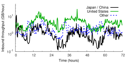
Figure 3: Inbound traffic for the JP data set split by geographic location

For the EU dataset only user traffic aggregates are available and no destination information was available to split traffic into TPGs. It would be a pessimistic assumption for TARDIS to simply split randomly as this would give each TPG the same temporal profile and reduce the opportunities for cost saving by space shifting (since each link would have its peak hour at the same time). Real traffic traces have different time behaviour for traffic originating from different destinations (for example P2P users turning off their client according to their local diurnal pattern). Therefore a means of splitting traffic was required which would induce slight difference in the diurnal cycle. The following procedure was used:

1. Half the traffic was split equally between each TPG.

2. The other half of the traffic was split between each TPG according to a weighted cosine function with 24 hour periodicity $\cos[(t-p_{i})*2\pi/24]$ where $t$ is the time period for the traffic being split (in hours) and $p_{i}$ is the time in hours hour where TPG $i$ gets peak weight.

This splitting process keeps the total amount of traffic in each hour the same but ensures that different TPGs have slightly different peaks by choosing different values for $p_{i}$. To evaluate the impact of the difference in the diurnal patterns between TPGs two different policies are used. In the policy $T_{2}$ the three TPGs have peak hours two hours apart and in $T_{4}$, four hours apart. Obviously, the more widely separated the peak hours, the better the system will perform under space shifting. Figure 4 shows inbound data for the EU dataset with the $T_{2}$ peak shift policy over the three hypothetical TPGs.

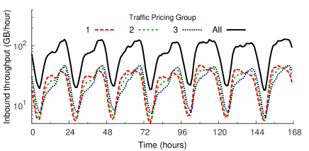
Figure 4: Inbound traffic for EU dataset split across three TPGs using $T_{2}$ weighting policy.

Having constructed hypothetical traffic pricing groups, it is now necessary to assign pricing schemes to each group. Hypothetical schemes were assumed to test a variety of scenarios (no real pricing data was available for the networks being tested). It will be assumed that traffic will be charged at the 95th percentile level on all TPGs, for the following pricing levels:

• Equal Prices, $P_{E}$, TPGs priced in the ratio 1:1:1.

• Low Variation, $P_{L}$, TPGs priced in the ratio 4:2:1.

• High Variation, $P_{H}$, TPGs priced in the ratio 10:3:1.

The high variation corresponds to “We set the unit traffic costs to be between $1 and $10 per Mbps, which corresponds to publicly available data on the current prices for Internet transit" [13].

6.2 Modelling user choice

The model discussed above can be used to determine how much demand a user places on traffic pricing groups for each time window. The next stage is to consider which other slots traffic may be shifted to. In practice, this will depend on technical feasibility, user willingness and the availability of data in another slot.

A question arises as to the correlation between traffic which can be shifted in time and traffic which can be shifted in space. If it were unlikely that time-shifting traffic could also space shift (because the two types were fundamentally different) then the two would be anti-correlated and this would mean that more traffic overall could shift than if there were no correlation. Conversely, it may be that the opposite is true and that traffic which can shift in time is more likely to be able to shift in space. If this is the case then less traffic will be able to shift at all than if there were no correlation. For the model we use we take the independence assumption as being a mid-way assumption.

An important problem in using the model in a practical context is generating the choice sets. To approach this problem systematically choice sets are generated separately for demand which can shift in time, demand which can shift in space and demand which can shift in both. For example, for space shifting, there must be a choice set for each time window containing slots for all TPGs. For time shifting within a given TPG, there must be a choice set for each time window which contains slots representing that TPG at that time window, the next time window, the time window after that, up to the maximum allowable delay shift. Although the number of choice sets is large, it is manageable as it is proportional to the product of the number of time windows and TPGs.

The user choice model selected can be condensed into the small set of parameters shown below.

$N_{T}$	Proportion of users eligible for time shifting.
$N_{S}$	Proportion of users eligible for space shifting.
$\mu_{T}$	Mean proportion of data shifted in time by eligible users.
$\mu_{S}$	Mean proportion of data shifted in space by eligible users.

Given these parameters, each user selects their time and space shifting characteristics as follows:

1. The ability to shift traffic in time or space is determined by comparing randomly generated numbers in (0,1) to thresholds $N_{T}$ and $N_{S}$ respectively.

2. For time shifting users, the proportion of time shifted data is set individually for each user to $P_{T}=R^{(1-\mu_{T})/\mu_{T}}$ where $R$ is a random number in (0,1). This produces a population of users who swap up to 100% of their traffic in time, with a mean proportion of $\mu_{T}$.

3. Similarly, for space shifting users, the proportion of space shifted data by each user is set to $P_{S}=R^{(1-\mu_{S})/\mu_{S}}$.

An assumption needs to be made about the maximum time delay allowed (here 18 hours was chosen) and which links are available for traffic to choose (here, it was chosen that traffic which could shift in space could always choose all three links). The combination of both available time windows and TPGs produces a choice set of available slots. For simplicity, traffic is treated identically within each slot. Given the available slots, the proportions $p_{ij}$ assigned by the dynamic model in section 5 are used to choose which slot to assign the traffic to. An amount of traffic $f$ can be assigned among slots in choice set $\mathcal{C}_{i}$ in two possible ways:

• All-or-nothing assignment. All of $f$ is assigned to a randomly chosen $j\in\mathcal{C}_{i}$ with probability $p_{ij}$.

• Proportional assignment. A proportion $p_{ij}$ of $f$ is assigned to each slot $j\in\mathcal{C}_{i}$.

6.3 Data analysis details

After the previous assumptions are made, the processing of data to assess the TARDIS algorithms is as follows:

1. Initialisation. A preliminary run through of all $N$ days of traffic is used to initialise the traffic splits $s_{ij}$ and to generate initial traffic profiles.

2. Pricing. Based on the traffic from the previous day, costs for each slot are calculated using the Shapley gradient procedure presented in section 4.

3. Traffic Shifting. The slot costs are used to update $s_{ij}$ for all slots in $\mathcal{C}_{i}$ as explained in section 5. Traffic assigned to each slot is updated accordingly.

4. Iteration. The next day is processed by returning to step 2. If day $N$ has been reached, processing continues by wrapping around to the first day, the second day and so on.

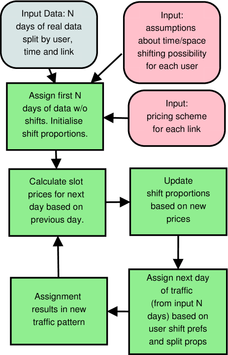
Figure 5: Diagram showing the trace driven analysis of TARDIS.

Figure 5 shows the analysis in diagramatic form. The known input is the $N$ days of traffic (from EU or from JP). This will include the assumptions $T_{0},T_{2}$ or $T_{4}$ from section 6.1 for the EU data and the geographic split for the JP data. Two assumed inputs are the time/space shifting possibilites (as discussed in section 6.2) and the pricing schemes. All pricing schemes tested here are 95th percentile (as that is the main focus of the Shapley gradient method) and the ratios between TPG are either $P_{H}$, $P_{L}$ or $P_{E}$ with $P_{H}$ the highest difference between links being the base case.

The analysis begins by modelling the traffic as if it could not choose slots for a warm up period. This initialises the shift proportions $s_{ij}$ for all choice sets $\mathcal{C}_{i}$. These are used to generate slot prices for the next day according to the Shapley gradient $G_{j}$ measured on the previous day’s traffic. The slot prices are used to update the shift proportions and these updated shift proportions are used to generate the next day of traffic in combination with the next day of traffic data from the EU or JP dataset.

Finally it is worth briefly mentioning execution time. The algorithm given is easily lightweight enough to run real time in practice for the number of users discussed here. The graphs in the next section each contain 25 graphs of 500 days and were run on only modest computing hardware. Each 500 day run took less than 1 day of real time to complete for 10,000 users. An implemented system would obviously have to perform only 1 day per day. It should also be noted that if the number of users is large then splitting rates can be calculated using only a sample of data. In fact the runs for the EU data were performed on a sample of 10,000 users – runs on the full data set produced extremely similar results. The runs for the JP data were performed on the full data set.

7 Analysis of user data

Results are presented in a common format. The simulation is run for 50 days as a “warm up" and then 500 simulated days. The effects of this recycling days is discussed in section 7.3. The split ratio is frozen for the final 50 days and the price paid over the first 50 days is compared with the price paid over the final 50 days. The graphs is repeated for different proportions of traffic being allowed to swap in time and in space. It is uncertain what proportions of traffic could in potential be engineered in this way so values from 0 to 60% are tried for space swapping and values from 0 to 20% for time swapping. The results are presented as the proportional reduction in price paid by the ISP and are compared to the theoretical maximum efficiency. The proportional reduction is given by $(P_{i}-P_{f})/P_{i}$ where $P_{i}$ is the mean daily price for the initial 50 day period and $P_{f}$ is the mean daily price for the final 50 day period. This ratio represents the reduction in price paid, e.g. 0.4 is a 40% saving. The theoretical maximum efficiency is simply the proportion of traffic which can swap either in time or in space. The data will not necessarily produce the same result on repeated runs as there are random elements to which users are assigned to swap and different users have different data profiles. Repeated tests with the same input are used to estimate the standard deviation on the obtained results and these are included on all plots. The exact procedure is described in section 7.3. Each box in the plots, therefore has the form $x\pm y(z)$ where $x$ is the calculated reduction in the price, $y$ is twice the estimated standard deviation (if the variable were normally distributed this would be a 95% confidence interval and $z$ is the reduction which would be achieved if all shifted traffic had zero cost. So, for example, $0.1\pm 0.02(0.14)$ should be interpreted as a cost reduction of 0.1 (10%) on the base costs with the true figure likely to be between 0.08 and 0.12 (the range being two standard deviations each side of the mean) and the maximum possible reduction (if all shifting traffic simply disappeared) being 0.14.

In all the cases tested here it is assumed that all three TPG are available for swapping. While this is an optimistic assumption, in many real situations more than three TPG would be available to an ISP. The high variation pricing scheme $P_{H}$ (i.e. a price ratio of 10:3:1) using 95th percentile pricing is the default for the base scenario. In addition, for the EU data set the base model includes the peak hour weighting scheme $T_{2}$ (see section 6.1.1). The base model uses the proportional assignment choice model (see section 6.2) but this was found to make no difference to the outcome (see section 7.3).

The proportion of time shifters is a combination of the proportion of users whose traffic shifts in time and the proportion of traffic shifted in time $N_{T}\mu_{T}$. Similarly for space shifting the proportion of traffic shifted in space is $N_{S}\mu_{S}$. To reduce the number of modelling parameters varied then $N_{T}=N_{S}=1$ and $\mu_{T}$ and $\mu_{S}$ are varied. However, the results were found to be no different if $\mu_{S}=\mu_{T}=1$ and $N_{T}$ and $N_{S}$ are varied (see section 7.3).

7.1 Base case results

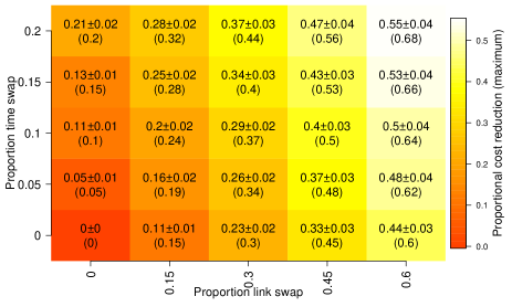
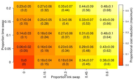
Figure 6: Base case for EU data (top) and JP data (bottom).

This section presents the results on the base case analysis. Figure 6 (top) shows the base case for the EU data. As can be seen, the savings are substantial with, in the highest case, 55% of the transit price being reduced. In many cases the saving is close to the optimal pricing that could occur. Note that in some cases it is slightly over due to statistical variances in the results (for example, if the traffic randomly selected to be allowed to shift happened to be on higher priced links in that run). It can be seen that, in particular, time shifting is extremely good at saving cost with almost all of the potential benefit being realised.

Figure 6 (bottom) shows the same results for the JP data. In this data there is more statistical variance in the results, likely because the data set has more “imbalance" in the traffic distribution with a small number of users contributing a large amount of data. Naturally, if those users move their data then this contributes more to the solution. The results show broadly the same pattern as the EU data but the link swapping is slightly less effective.

7.2 Variant results

A number of variants on the base scenario were tried and are reported here. The most obvious variant is to try the lower difference in pricing. In this scenario the link prices are split in the ratio 4:2:1 not 10:3:1. The results are presented in figure 7. The effectiveness of time swapping is not reduced significantly as might be expected. However, the effectiveness of link swapping remains relatively high, especially in scenarios with low levels of time swapping. Therefore it seems link swapping can still be extremely effective for saving cost even when cost differences are low. In fact there was still some leeway Nonetheless, in this scenario, in the cast with most swappers, almost 40% of the price is saved in both data sets (the theoretical maximum being 68%). In fact tests on the equal price policy $P_{E}$ show that by taking advantage of the peak time differences gains can be made even when there is no difference between the rates charged. For example on the JP data set a cost saving of 10% was made in a scenario with 20% space shifting and no time shifting.

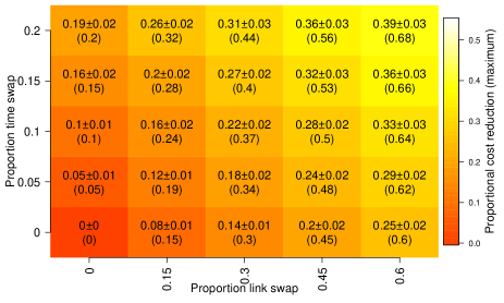
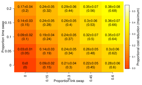
Figure 7: Low pricing variant case for EU data (top) and JP data (bottom).

An investigation was made into the effect of a wider split in the peak hours across pricing groups, the $T_{4}$ scenario described in section 6.1.1. As would be expected, this produces some advantage for the TARDIS system but in fact the advantage is slight and the results are indistinguishable from the $T_{2}$ results when error bars are accounted for. The graph for the EU data is shown in figure 8. When compared with figure 6 (top) it is apparent that little difference to the price has been made.

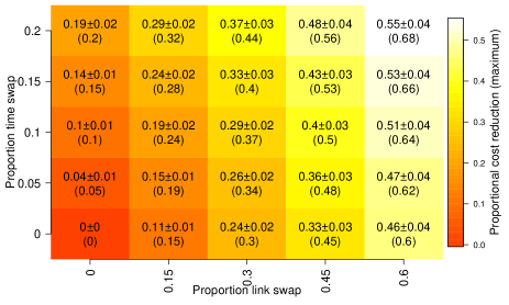
Figure 8: The $T_{4}$ variant in traffic splits, EU data

7.3 Checking data analysis assumptions

A number of assumptions on the data analysis are checked for robustness. The first, and most important, is the repeatability of runs. As mentioned, the stochastic element to assignment of which traffic can be swapped means that not every run gets the same results even with identical input. It is therefore important to calculate the repeatability of the results. This is assessed by a run with 60% link swappers and 20% time swappers repeated ten times each for the JP and EU data. The Shapiro-Wilk normality test showed that the results were not normally distributed and no simple distribution could be found hence no simple way of calculating confidence intervals was available. Instead the coefficient of variation is calculated (the ratio of standard deviation to mean). This is used to calculate estimated standard deviations for the results.

Runs were made with prices on all links equal. Benefits from swapping in space were still present as different links had different peak times. The exception was in the EU data set if policy $T_{0}$ was used to split traffic between links. In the case of exactly equal traffic on all links and equal prices on all links then no benefit was discovered from link swapping, as might be expected. With equal prices, 20% of link swappers and no time swappers produced a 5% saving in prices in the EU data (with the $T_{2}$ policy) and 10% in the JP data.

Runs were made to test assumptions about which traffic was chosen to shift. No significant difference was found in the results when $x\%$ of users were chosen to shift all their traffic or when all users were chosen to shift $x\%$ of their traffic (chosen at random).

Runs were made to test assumptions about the limited number of days of data available. In specific it might be worried that the very good performance on the data was due to the same data being recycled again and again. To test this artificial extra days were generated from the real days of data by the following procedure.

1. A total traffic level for the new day is chosen from a normal distribution with the same mean and variance as the real traffic’s daily traffic level.

2. Each user picks one day at random and uses their traffic profile for that day.

3. The traffic for each user is multiplied by a constant chosen to give the required traffic level from the first step.

This procedure will generate extra days of traffic which have the same mean traffic level and same variance in traffic level between days as the original and will also have the same split of traffic between users as the original. However, every day of traffic will be different. By using this procedure then it is certain that cost savings are not due to the traffic being “too predictable". Conversely, however, the traffic levels for the assessment days can increase or decrease (about a constant mean) so a perceived cost saving or increase could be a result of a temporary increase in traffic. Figure 9 shows these results for the JP data set. This should be compared with figure 6 (bottom). The errors are larger on this graph because of the fluctuation on the data. This can be seen especially in the base case with zero time and space shifting where the cost has got worse even though no users can shift. This is simply a random fluctuation upwards in traffic. The two standard deviation bound is larger in this graph because it includes elements for the repeatability of the assignment procedure but also variations in the traffic levels. There appears to have been a decline in the benefit in some scenarios this is within the two standard deviation bounds so it is hard to tell whether it is a real variation or a result of random traffic growth. For example $0.48\pm 0.1$ in the base case has become $0.41\pm 0.14$ in the case with varying traffic. Most falls are of around this level so if the variation in the traffic is causing worse performance it seems that it is not greatly worse.

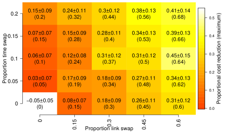
Figure 9: The JP results with randomised “extra" days of traffic.

Finally, the outcomes of using either the all-or-nothing or proportional allocation strategies (see section 6.2) were also tested. No significant differences were found between the two.

7.4 Discussion and criticism of results

It is hard to get realistic results to assess the TARDIS system for several reasons. Firstly, it is hard to get data sets for several days of data which maps ingress and egress traffic to individual users (ideally in a non-anonymised way the lack of anonymisation is what enabled separation of the JP traffic by destination). Publicly available traces known to the researchers were unsuitable for one or more of these reasons and hence non public data had to be used. Secondly, ISP pricing plans are commercially sensitive and not usually publicly disclosed. Findally, knowledge of the likely traffic which can be shifted is hard to get. The percentage shifting in space can only be estimated from work such as [1, 6, 14], estimates seem to be relatively high ([6] gives 40% of traffic available in three or more locations). Knowledge of which traffic can be time shifted is even less available although some insights can be gained from work such as [10, 9].

In the light of these problems, the results in this section are an attempt to get the best possible assessment of the system without introducing too many parameters which cannot be estimated. They should be taken as an investigation of how well the system is likely to work under a range of conditions and a robust attempt to locate potential areas where the assumptions would cause problems for such a system in practice. The large scale of the traces meant that each investigation took considerable computing time (This is because of the necessity of simulating the behaviour of tens of thousands of users for every day simulated, a real TARDIS system would only have to calculate splitting rates which is a much easier task.)

This said, the results are remarkably successful in all the system variants investigated here. In the majority of cases the TARDIS system extracted a high proportion of the maximum possible benefit available. Even when the assumptions were relatively conservative (a low variation in pricing between transit links, a small percentage of traffic able to swap in space or in time) the benefit in terms of cost saving could still be relatively large.

With more detailed knowledge of ISP pricing and internal network structures the scheme could be tested on its ability to reduce transit costs while retaining the constraints of limited traffic capacities on internal links or while avoiding causing excess congestion in downstream systems.

8 Conclusions

This paper introduced TARDIS (Traffic Assignment and Retiming Dynamics with Inherent Stability) an algorithm for determining how to reassign traffic in time and space to reduce ISP transit costs. A method was given to assign a cost to a given link at a given time of day according to any of a number of widely used pricing schemes. This time of day cost was used as an input to a reassignment scheme for traffic. Modelling the scheme as a dynamical system it was shown that a continuous approximation to the scheme was provably stable and assigned traffic to an equilibrium situation.

The scheme was tested in a realistic context by analysis of real life data sets. This analysis tested several different assumptions about pricing levels and about proportions of traffic space and time shifting. In the majority of cases a large financial saving is possible. Time shifting appears to create a considerable saving in most situations. Space shifting creates a saving in all situations except those where all links are equally priced and traffic is split equally across all links.

This research has received funding from the Seventh Framework Programme (FP7/2007-2013) of the European Union, through the FUSION project (grant agreement 318205).

Appendix A The Shapley gradient price

In section 4.2 the Shapley gradient $G_{j}$ was introduced as the cost gradient of the Shapley value when a fictitious user $N+1$ adds an amount of traffic $du$ to slot $j$. Define the per user Shapley gradient for user $i$ in slot $j$ as $\phi^{\prime}_{ij}=(\phi_{i}(d_{ij})-\phi_{i})/du$ where $\phi_{i}(d_{ij})$ is the Shapley value for user $i$ with extra traffic $du$ in slot $j$. It was stated that for all schemes considered in this paper then the mean over $i$ of $\phi^{\prime}_{ij}$ is $G_{j}$. In the simplest cases, $\phi^{\prime}_{ij}=G_{j}$ for all $i$.

Formally, from section 4.2

$$G_{j} =\frac{1}{du\,(N+1)!}$$

$$\sum_{\pi\in\mathcal{S}_{\mathcal{N}^{\prime}}}[v(\mathcal{S}(\pi,N+1))-v(\mathcal{S}(\pi,N+1)\backslash N+1)],$$

where $\mathcal{S}_{\mathcal{N}^{\prime}}$ is the set of arrangements of the users $\mathcal{N}$ plus the fictitious $(N+1)$th user and $\mathcal{S}(\pi,N+1)$ is the set of all users arriving not later than user $N+1$ in the permutation $\pi$.

For linear pricing this is trivial to show. If the slot $j$ is charged at rate $r_{j}$ then $\phi_{i}(d_{ij})-\phi_{i}=r_{j}du$ since the extra traffic $du$ costs $r_{j}du$. Hence, $\phi^{\prime}_{ij}=r_{j}$ and is not dependent on $i$. It is already shown in section 4.3.1 that $G_{j}=r_{j}$.

For the pricing of a link of fixed capacity as described in section 4.3.4 then the case is very similar. The price depends only on the total flow on the link. So

$$\phi_{i}(d_{ij})-\phi_{i} =\frac{f_{j}+du-\alpha m}{m-(f_{j}+du)}-\frac{f_{j}-\alpha m}{m-f_{j}}$$

$$=\frac{(1-\alpha)m\,du}{(m-f_{j})(m-(f_{j}+du))}$$

$$=\frac{(1-\alpha)m\,du}{(m-f_{j})^{2}},$$

where the final equality is because $du$ is infinitesimal with respect to $f_{j}$. Hence $\phi^{\prime}_{ij}=G_{j}=\frac{(1-\alpha)m}{(m-f_{j})^{2}}$ as calculated in section 4.3.4. Any scheme where the price does not depend on the user could be analysed in a similar manner.

For the 95th percentile pricing then by the arguments from section 4.3.2

$$\phi^{\prime}_{ij}=(\phi_{i}(d_{ij})-\phi_{i})/du=\frac{1}{N!}\sum_{\pi\in\mathcal{S}_{\mathcal{N}}}[F_{ij}],$$

where

$$F_{ij} =[v(\mathcal{S}(\pi,i))+I(j\in\mathcal{T}^{(95)}(\mathcal{S}(\pi,i))r_{j}\,du$$

$$\quad-v(\mathcal{S}(\pi,i)\backslash i)]/du-[v(\mathcal{S}(\pi,i))-v(\mathcal{S}(\pi,i)\backslash i)]/du$$

$$=I(j\in\mathcal{T}^{(95)}(\mathcal{S}(\pi,i))r_{j}.$$

The mean of $\phi^{\prime}_{ij}$ over all users $i$, $\overline{\phi^{\prime}_{ij}}$ is given by:

$$\overline{\phi^{\prime}_{ij}}=\sum_{i=1}^{N}\frac{\phi^{\prime}_{ij}}{N}=\frac{1}{NN!}\sum_{i=1}^{N}\sum_{\pi\in\mathcal{S}_{\mathcal{N}}}I(j\in\mathcal{T}^{(95)}(\mathcal{S}(\pi,i))r_{j}.$$

Now notice that $\sum_{\pi\in\mathcal{S}_{\mathcal{N}}}$ covers all arrangements of $N$ items and $I(j\in\mathcal{T}^{(95)}(\mathcal{S}(\pi,i))$ covers all occasions where an addition of traffic $du$ following user $i$ falls in the 95th percentile set for $\mathcal{S}(\pi,i)$. As this is summed over all values of $i$ this is exactly the same as considering those occasions where the $N+1$th user (who adds traffic $du$ to slot $j$) follows any other user over any arrangement of users in $\mathcal{N}^{\prime}$ (the set of users 1 to $N$ plus the fictitious user $N+1$). This includes every possible arrangement of users in $\mathcal{N}^{\prime}$ except those with user $N+1$ first. Therefore

$$\sum_{i=1}^{N}\frac{\phi^{\prime}_{ij}}{N} =\frac{r_{j}}{NN!}\sum_{\pi\in\mathcal{S}_{\mathcal{N}^{\prime}}}[v(\mathcal{S}(\pi,N+1))$$

$$\quad-v(\mathcal{S}(\pi,N+1)\backslash N+1)]$$

$$=\frac{N+1}{N}\frac{r_{j}}{(N+1)!}\sum_{\pi\in\mathcal{S}_{\mathcal{N}^{\prime}}}[v(\mathcal{S}(\pi,N+1))$$

$$\quad-v(\mathcal{S}(\pi,N+1)\backslash N+1)]$$

$$=\frac{N+1}{N}G_{j}.$$

As $N$ becomes large $(N+1)/N\rightarrow 1$ and hence the mean over $i$ of $\phi^{\prime}_{ij}$ becomes closer to $R_{j}$. More precisely $\overline{\phi^{\prime}_{ij}}=R_{j}+O(1/N)$ as stated in section 4.3.2.

Appendix B A stability proof for multiple choice sets

Theorem 1 is identical to that in the appendix of [16] with the exception of condition (3) which in that reference is given for a single vector $\mathbf{x}$ as $\nabla V(\mathbf{x})\cdot\Phi(\mathbf{x})<0$, in the theorem here is given over several vectors as $\nabla_{i}V(\mathbf{x}_{i})\cdot\Phi(\mathbf{x}_{i})<0$ where $\nabla_{i}$ is the gradient over the vector space of $\mathcal{C}_{i}$, that is

$$\nabla_{i}(\mathbf{x})=(\partial\mathbf{x}/X_{i\,1},\partial\mathbf{x}/X_{i\,2},\ldots).$$

Recall that $\mathbf{D}$ is the set of $X_{ij}$ which are demand feasible (that is $\sum_{j}X_{ij}=d_{i}$ for all $i$). Intuitively, this says that the demand which must be assigned to choice set $\mathcal{C}_{i}$ is equal to the sum of the demand which is actually assigned. It is important to note that the demand feasible set is decomposable by choice set in the sense that the matrix $X$ is demand feasible if and only if each of its rows $\mathbf{x}_{i}$ is. Therefore, let $\mathbf{x}_{i}$ be demand feasible if $\sum_{j}X_{ij}=d_{i}$ and (slightly abusing the notation) say that $\mathbf{x}_{i}\in\mathbf{D}$. For points on the trajectory of the dynamical system then $\accentset{\mbox{\large.}}{\mathbf{X}}=\Phi(\mathbf{X})$ and therefore, for all $i$ then $\accentset{\mbox{\large.}}{\mathbf{x}_{i}}=\Phi(\mathbf{x}_{i})$.

Having established that a demand $\mathbf{X}\in\mathbf{D}$ must be composed of vectors $\mathbf{x}_{i}$ all of which themselves are demand feasible ($\mathbf{x}_{i}\in\mathbf{D}$) then the proof now follows that in the appendix of [16] for each $\mathbf{x}_{i}$ component separately. This shows that each choice set individually converges to its equilibrium condition and hence the entire system converges.

In brief the proof in [16] follows an epsilon delta style argument. Firstly a set $\mathbf{D}_{\epsilon}$ is defined as the set of demand feasible points $\mathbf{x}\in\mathbf{D}$ with $V(\mathbf{x})>\epsilon$ for some $\epsilon>0$. It is then shown that if the system starts at a position $\mathbf{x}\in\mathbf{D}_{\epsilon}$ and the dynamical system evolves following $\accentset{\mbox{\large.}}{\mathbf{x}}=\Phi(\mathbf{x})$ and stays within $\mathbf{D}_{\epsilon}$ until some time $T$ then there is some fixed $\delta>0$ for which $\nabla V(\mathbf{x})\cdot\Phi(\mathbf{x})<-\delta$. Let $\mathbf{x}(t)$ represent the system state at time $t$. The function $V(\mathbf{x})$ must shrink at least at rate $\delta$ and hence $V(\mathbf{x}(T))-V(\mathbf{x}(0))<-\delta T$. Therefore $V(\mathbf{x}(t_{0}))<\epsilon$ for some finite $t_{0}\leq V(\mathbf{x}(0))/\delta$. In other words the points leave $\mathbf{D}_{\epsilon}$ within some finite time whatever the size of $\epsilon$. Since this argument applies for all $\epsilon$ then as $\epsilon\rightarrow 0$ the set $\mathbf{D}_{\epsilon}$ covers all of $\mathbf{D}$ except for the equilibrium positions where $V(\mathbf{X})=0$.

It is now necessary to show that the candidate $V(\mathbf{x}_{i})$ meets the three conditions of Theorem 1. Recall from section 5.2 that the candidate functions are

$$V(\mathbf{x}_{i})=\sum_{j,k\in\mathcal{C}_{i}}X_{ij}(p_{k}-p_{j})_{+}^{2}.$$

The first two conditions are trivially shown. Firstly, $V(\mathbf{x}_{i})\geq 0$ since both $X_{ij}\geq 0$ and $(p_{j}-p_{k})_{+}^{2}\geq 0$. Secondly $V(\mathbf{x}_{i})=0$ only when $\mathcal{C}_{i}$ is at equilibrium. This follows from the definition of equilibrium. If some term is non zero then $X_{ij}>0$ and $p_{j}>p_{k}$ for some $j,k\in\mathcal{C}_{i}$ then this implies there is a flow $X_{ij}$ in choice set $\mathcal{C}_{i}$ which has a price $p_{j}$ greater than some $p_{k}$ also in $\mathcal{C}_{i}$. This is counter to the definition of equilibrium in definition 1.

The final condition (3) of the theorem is the most difficult and again the proof follows [16] but generalised to several choice sets.

Begin by differentiating $V(\mathbf{x}_{i})$ by parts. Define $\Delta_{ijk}$ as a vector with $-1$ in position $j$ and $+1$ in position $k$ if $j,k\in\mathcal{C}_{i}$ and the zero vector if either $j\notin\mathcal{C}_{i}$ or $k\notin\mathcal{C}_{i}$. Define $\mathbf{p}$ as the price vector $\mathbf{p}(\mathbf{X})=(p_{1}(\mathbf{X}),p_{2}(\mathbf{X}),\ldots)$. In this form, then $V(\mathbf{x}_{i})=\sum_{j,k\in\mathcal{C}_{i}}X_{ij}(p_{j}-p_{k})_{+}^{2}$ can be written more compactly as $V(\mathbf{x}_{i})=\sum_{j,k}-X_{i\,j}\,(\mathbf{p}(\mathbf{X})\cdot\Delta_{ijk})_{+}^{2}$ (where the sum is over all flows in $\mathbf{X}$ and $\cdot$ is the inner product). Considering $\Phi(\mathbf{x}_{i})=(\accentset{\mbox{\large.}}{X_{i\,1}},\accentset{\mbox{\large.}}{X_{i\,2}},\ldots)$ the elements

$$\accentset{\mbox{\large.}}{X_{ij}}=\sum_{k\in\mathcal{C}_{i}}\left[X_{ik}(p_{k}-p_{j})_{+}-X_{ij}(p_{j}-p_{k})_{+}\right]$$

can be written as as

$$\accentset{\mbox{\large.}}{X_{ij}}=\sum_{k}X_{ij}(\mathbf{p}(\mathbf{X})\cdot\Delta_{ijk})_{+}-X_{ik}(\mathbf{p}(\mathbf{X})\cdot\Delta_{ijk})_{+}.$$

Performing the differentiation $\nabla_{i}V(\mathbf{x}_{i})$ by parts gives

$$\nabla_{i}V(\mathbf{x}_{i}) =\sum_{j,k}-2X_{ij}\,(\mathbf{p}(\mathbf{X})\cdot\Delta_{ijk})_{+}\nabla_{i}(\mathbf{p}(\mathbf{X})\cdot\Delta_{ijk})_{+}$$

$$\quad-\nabla_{i}(X_{ij})(\mathbf{p}(\mathbf{X})\cdot\Delta_{ijk})_{+}^{2}$$

$$=-2\mathbf{J}_{i}\Phi(\mathbf{x}_{i})^{T}-\sum_{j,k}(\mathbf{p}(\mathbf{X})\cdot\Delta_{ijk})_{+}^{2}\mathbf{e}_{ij},$$

where $\mathbf{e}_{ij}$ is the basis vector in the space of $\mathcal{C}_{i}$ which is 0 except for a 1 in the direction of $X_{ij}$ and $\mathbf{J}_{i}$ is the Jacobian of the price matrix at $\mathbf{X}$ in the vector space $\mathcal{C}_{i}$ given by

$$\mathbf{J}_{i}=\left[\begin{array}[]{ccc}\partial p_{1}(\mathbf{X})/\partial X_{i\,1}&\partial p_{1}(\mathbf{X})/\partial X_{i\,2}&\cdots\\ \partial p_{2}(\mathbf{X})/\partial X_{i\,1}&\partial p_{2}(\mathbf{X})/\partial X_{i\,2}&\cdots\\ \vdots&\vdots&\ddots\end{array}\right].$$

Hence

$$\nabla_{i}V(\mathbf{x}_{i})\cdot\Phi(\mathbf{x}_{i}) =-2\Phi(\mathbf{x}_{i})\mathbf{J}_{i}\Phi(\mathbf{x}_{i})^{T}$$ (6)

$$\quad-\sum_{j,k}(\mathbf{p}(\mathbf{X})\cdot\Delta_{ijk})_{+}^{2}\sum_{l,m}(\mathbf{p}(\mathbf{X})(\mathbf{e}_{ij}\cdot\Delta_{ilm}).$$

One of the conditions on $\mathbf{J}_{i}$ (the rate of change of the price) was that it was monotonically non decreasing (condition 2 in section 4). Hence $\mathbf{X}\mathbf{J}_{i}\mathbf{X}^{T}\geq 0$ for all $X$. Thus $-2\Phi(\mathbf{x}_{i})\mathbf{J}_{i}\Phi(\mathbf{x}_{i})^{T}<0$.

It can also be shown that $-\sum_{j,k}(\mathbf{p}(\mathbf{X})\cdot\Delta_{ijk})_{+}^{2}\sum_{l,m}(\mathbf{p}(\mathbf{X})(\mathbf{e}_{ij}\cdot\Delta_{ilm}\leq 0$ following [16] again by showing that the remaining term in $\nabla V(\mathbf{x}_{i})\cdot\Phi(\mathbf{x}_{i})$, given by

$$-\sum_{j,k}(\mathbf{p}(\mathbf{X})\cdot\Delta_{ijk})_{+}^{2}\sum_{l,m}(\mathbf{p}(\mathbf{X})(\mathbf{e}_{ij}\cdot\Delta_{ilm})<0.$$

Since both terms in (6) are less than zero then this gives that $\nabla V(\mathbf{x}_{i})\cdot\Phi(\mathbf{x}_{i})<0$ for all $i$ as required.

References

- [1] B. Ager, W. Mühlbauer, G. Smaragdakis, and S. Uhlig. Web content cartography. In Proc. of ACM/SIGCOMM IMC, pages 585–600, 2011.
- [2] D. Antoniades, E. P. Markatos, and C. Dovrolis. One-click hosting services: a file-sharing hideout. In Proc. of ACM/SIGCOMM IMC, pages 223–234, 2009.
- [3] P. Chhabra, N. Laoutaris, P. Rodriguez, and R. Sundaram. Home is where the (fast) internet is: Flat-rate compatible incentives for reducing peak load. In Proceedings of ACM HomeNETS, 2010.
- [4] D. R. Choffnes and F. E. Bustamante. Taming the torrent: a practical approach to reducing cross-ISP traffic in peer-to-peer systems. In Proc. of ACM SIGCOMM, 2008.
- [5] X. Dimitropoulos, P. Hurley, A. Kind, and M. P. Stoecklin. On the 95-percentile billing method. In Proc. of PAM, 2009.
- [6] B. Frank, I. Poese, G. Smaragdakis, S. Uhlig, and A. Feldmann. Content-aware Traffic Engineering. In Proceedings of ACM SIGMETRICS/Performance 2012, London, UK, June 2012.
- [7] D. K. Goldenberg, L. Qiuy, H. Xie, Y. R. Yang, and Y. Zhang. Optimizing cost and performance for multihoming. In Proc. of ACM SIGCOMM, pages 79–92, 2004.
- [8] W. Jiang, R. Zhang-Shen, J. Rexford, and M. Chiang. Cooperative content distribution and traffic engineering in an ISP network. In ACM SIGMETRICS, 2009.
- [9] C. Joe-Wong, S. Ha, and M. Chiang. Time-dependent broadband pricing: Feasibility and benefits. In Proc. of IEEE ICDCS, 2011.
- [10] C. Joe-Wong, S. Ha, and M. Chiang. Time-dependent internet pricing. In Proc. of Internet Technologies and Applications Conference (ITA), 2011.
- [11] A. Katok and B. HasselBlatt. Introduction to the Modern Theory of Dynamical Systems. Cambridge University Press, 1995.
- [12] N. Laoutaris and P. Rodriguez. Good things come to those who (can) wait: or how to handle Delay Tolerant traffic and make peace on the internet. In Proc. of ACM HotNets, 2008.
- [13] M. Motiwala, A. Dhamdhere, N. Feamster, and A. Lakhina. Towards a cost model for network traffic. SIGCOMM Comput. Commun. Rev., 42(1):54–60, 2012.
- [14] I. Poese, B. Frank, B. Ager, G. Smaragdakis, and A. Feldmann. Improving content delivery using provider-aided distance information. In Proc. of ACM/SIGCOMM IMC, pages 22–34, 2010.
- [15] R. C. Rumin, N. Laoutaris, X. Yang, G. Siganos, and P. Rodriguez. Deep diving into bittorrent locality. In Proc. of IEEE INFOCOM, 2011.
- [16] M. J. Smith. The stability of a dynamic model of traffic assignment – an application of a method of Lyapunov. Transp. Science, 18(3):245–252, 1984.
- [17] R. Stanojevic, N. Laoutaris, and P. Rodriguez. On economic heavy hitters: Shapley value analysis of 95th percentile pricing. In Proc. of ACM/SIGCOMM IMC, 2010.
- [18] V. Valancius, C. Lumezanu, N. Feamster, R. Johari, and V. Vazirani. How many tiers? pricing in the internet transit market. In Proc. of ACM SIGCOMM, 2011.
- [19] J. G. Wardrop. Some theoretical aspects of road traffic research. Proc. of the Inst. of Civil Engineers II, 1:325–378, 1952.
- [20] H. Xie, Y. R. Yang, A. Krishnamurthy, Y. Liu, and A. Silverschatz. P4P: Provider portal for applications. In Proc. of ACM SIGCOMM, 2008.