Ultrarigid periodic frameworks

Abstract

We give an algebraic characterization of when a $d$-dimensional periodic framework has no non-trivial, symmetry preserving, motion for any choice of periodicity lattice. Our condition is decidable, and we provide a simple algorithm that does not require complicated algebraic computations. In dimension $d=2$, we give a combinatorial characterization in the special case when the the number of edge orbits is the minimum possible for ultrarigidity. All our results apply to a fully flexible, fixed area, or fixed periodicity lattice.

1.  Introduction

A periodic framework is an infinite structure in Euclidean $d$-space, made of fixed-length bars connected by universal joints and symmetric with respect to a lattice $\Gamma$. To fully describe the model, we need to describe the allowed motions. The Borcea-Streinu deformation theory [7], by-now the standard in the mathematical literature on periodic frameworks, allows precisely those motions which preserve the lengths and connectivity of the bars and symmetry with respect to $\Gamma$, but not the geometric representation of $\Gamma$, which is allowed to deform continuously. We give more detail shortly, in Section 1.1, but want to call out here the key features of forced symmetry and deformable lattice representation.

For this setting there are good algebraic [7] and, in dimension $2$, combinatorial [27] characterizations of rigidity and flexibility. Simply dropping the symmetry forcing altogether is known to lead to quite complicated behavior [31], and the tools from [7, 27] do not apply directly. One alternative approach is to study the behavior when relaxing the symmetry constraints along a decreasing sequence of sublattices. In this paper, we will consider the extreme case, characterizing the periodic frameworks that are infinitesimally rigid and remain so when the symmetry constraint is relaxed to any sublattice.

1.1  The basic setup and background

A periodic framework is defined by the triple $(\tilde{G},\varphi,\tilde{\bm{\ell}})$, where $\tilde{G}$ is an infinite graph, $\varphi:\mathbb{Z}^{d}\to\operatorname{Aut}(G)$ is a free $\mathbb{Z}^{d}$-action with finite quotient, and $\tilde{\bm{\ell}}:E(\tilde{G})\to\mathbb{R}_{>0}$ is a $\varphi$-equivariant function assigning a length to each edge. A realization $(\mathbf{p},\mathbf{L})$ of $(\tilde{G},\varphi,\tilde{\bm{\ell}})$ is given by a function $\mathbf{p}:V(\tilde{G})\to\mathbb{R}^{d}$ and a matrix $\mathbf{L}\in\mathbb{R}^{d\times d}$ such that $\mathbf{p}$ is equivariant with respect to the lattice generated by the columns of $\mathbf{L}$, i.e.,

$$\begin{array}[]{rcll}||\mathbf{p}(j)-\mathbf{p}(i)||^{2}&=&\tilde{\bm{\ell}}(ij)^{2}&\text{for all $ij\in E(\tilde{G})$}\\ \mathbf{p}(\varphi(\gamma)(i))&=&\mathbf{p}(i)+\mathbf{L}\cdot\gamma&\text{for all $i\in V(\tilde{G})$ and $\gamma\in\mathbb{Z}^{d}$}\end{array}$$

Realizations are denoted by $\tilde{G}(\mathbf{p},\mathbf{L})$. The set of all realizations is denoted $\mathcal{R}(\tilde{G},\varphi,\tilde{\bm{\ell}})$, and the configuration space $\mathcal{C}(\tilde{G},\varphi,\tilde{\bm{\ell}})=\mathcal{R}(\tilde{G},\varphi,\tilde{\bm{\ell}})/\operatorname{Euc}(d)$ is then defined as the quotient of the realization space by Euclidean isometries. A realization $\tilde{G}(\mathbf{p},\mathbf{L})$ is then rigid if it is isolated in the configuration space and otherwise flexible. The realization $\tilde{G}(\mathbf{p},\mathbf{L})$ is infinitesimally rigid if the tangent space at $(\mathbf{p},\mathbf{L})$ in $\mathcal{R}(\tilde{G},\varphi,\tilde{\bm{\ell}})$ is $d+1\choose 2$-dimensional and otherwise infinitesimally flexible.

The essential results on this model from [7], which introduced it, are that: (i) the realization and configuration spaces are finite-dimensional algebraic varieties; (ii) generically, rigidity and flexibility are determined completely by the absence or presence of a non-trivial infinitesimal flex, which can be tested for in polynomial time via linear algebra; (iii) generic rigidity and flexibility are properties of the finite colored quotient graph of $(G,\bm{\gamma})$, which is a finite directed graph, with its edges labeled by elements of $\mathbb{Z}^{d}$. (See Section 2 for the dictionary between infinite periodic graphs and colored graphs.)

In dimension two, [27, Theorem A], gives a combinatorial characterization of generic periodic rigidity, in terms of the colored quotient graph. The characterization is a good one, in the sense that it is decidable by polynomial-time, combinatorial algorithms. For higher dimensions, as is also the case for finite bar-joint frameworks, finding a similar combinatorial characterization is a notable open problem.

All of the above-mentioned results on periodic frameworks rely, in an essential way, on symmetry-forcing. Simply dropping the symmetry requirements for the allowed motions leads to configuration spaces that are not treatable via the techniques from [7]. Additionally, starting with a rigid periodic framework $\tilde{G}(\mathbf{p},\mathbf{L})$ and relaxing the symmetry constraint to any sublattice at all produces a framework that is, a priori, non-generic, and so we cannot naively apply the results of [7, 27] to it.

1.2  Ultrarigidity

We define a periodic framework $\tilde{G}(\mathbf{p},\mathbf{L})$ to be periodically ultrarigid (simply ultrarigid, for short, since there is no chance of confusion) if it is rigid and remains so after relaxing the symmetry constraint to any sublattice. This definition and terminology are from [4]. That not all infinitesimally rigid periodic frameworks are ultrarigid was observed in [7]. The question of which colored graphs are generically ultrarigid was raised, for dimension $2$, in [44] under the name “sublattice question”. A similar question for periodic frameworks in all dimensions was raised in [36, Question 8.2.7].

For any sublattice $\Lambda<\mathbb{Z}^{d}$, one can compute an associated rigidity matrix whose kernel is the space of infinitesimal motions periodic relative to $\Lambda$. However, this does not provide a formulation that immediately provides a finite certificate of infinitesimal ultrarigidity. One must, a priori, compute the rank of infinitely many matrices. (A finite certificate of infinitesimal “ultraflexibility” is given simply by the rigidity matrix associated with a particular sublattice that yields a non-trivial infinitesimal motion.)

1.3  Results and roadmap

Our main theorem is an effective algebraic characterization of infinitesimal ultrarigidity. To state it, we first recall that a torsion point in $(\mathbb{C}^{\times})^{d}=(\mathbb{C}\setminus\{0\})^{d}$ is any point $\omega=(\zeta_{1},\dots,\zeta_{d})\in\mathbb{C}^{d}$ where $\zeta_{1},\dots,\zeta_{d}$ are roots of unity. Equivalently, a torsion point is any point with finite order in the group $(\mathbb{C}^{\times})^{d}$ where the group operation is component-wise multiplication. Let $\mathbf{1}=(1,1,\dots,1)$

Theorem 1.

Let $\tilde{G}(\mathbf{p},\mathbf{L})$ be an infinitesimally rigid periodic framework in dimension $d$, with colored quotient graph $(G,\bm{\gamma})$. Then there is an explicit constant $N(d,G,\mathbf{p},\mathbf{L})$ depending only on $d,G,\mathbf{p},\mathbf{L}$, and a finite collection of polynomials $p_{1},p_{2},\ldots,p_{k}\in\mathbb{C}[x_{1},x_{2},\ldots,x_{d}]$ such that $\tilde{G}(\mathbf{p},\mathbf{L})$ is infinitesimally ultrarigid if and only if $\mathbf{1}$ is the only torsion point of order $\leq N(d,G,\mathbf{p},\mathbf{L})$ in the common solution set of $p_{1},p_{2},\ldots,p_{k}$. If $\mathbf{p},\mathbf{L}$ are rational, we can replace $c(d,G,\mathbf{p},\mathbf{L})$ with a constant $c(d,G)$ depending only on $d,G$.

Theorem 1 follows directly from: a characterization of infinitesimal ultrarigidity from which the polynomials $p_{i}$ are derived (Theorem 2 below); and a general theorem regarding torsion points as common solutions to polynomials of bounded degree (Theorem 3 below).

1.3.1.  Infinitesimal ultrarigidity

The polynomials $p_{i}$ are given by minors of a matrix $\hat{S}_{G,\mathbf{d}}$ with entries in the group ring $\mathbb{R}[\mathbb{Z}^{d}]$ with the pattern

$$\bordermatrix{&&i&&j&\cr&\dots&\dots&\dots&\dots&\dots\cr ij&\dots&-\mathbf{d}_{ij}&\dots&\mathbf{d}_{ij}\otimes\gamma_{ij}&\dots\cr&\dots&\dots&\dots&\dots&\dots}$$ (1)

where $\mathbf{d}_{ij}=\mathbf{p}_{j}-\mathbf{p}_{i}+\mathbf{L}\cdot\mathbf{\gamma}_{ij}$ is the edge vector associated with the colored edge $ij\in E(G)$, $\gamma_{ij}$ is viewed as an element of the group ring, and $\otimes$ denotes component-wise multiplication.

We can view $\hat{S}_{G,\mathbf{p},\mathbf{L}}$ as a matrix with monomial entries in $\mathbb{R}[x_{1},x_{1}^{-1},\dots,x_{d},x_{d}^{-1}]$ via the natural isomorphism $\mathbb{R}[\mathbb{Z}^{d}]\to\mathbb{R}[x_{1},x_{1}^{-1},\dots,x_{d},x_{d}^{-1}]$ defined by $\gamma\mapsto x^{\gamma}:=x_{1}^{\gamma_{1}}x_{2}^{\gamma_{2}}\cdots x_{d}^{\gamma_{d}}$ where $\gamma_{i}$ are the components of $\gamma$. That this rigidity matrix captures the infinitesimal motions is the first part of the proof of Theorem 1, and it follows from:

Theorem 2 (name=[9, 32]).

Let $\tilde{G}(\mathbf{p},\mathbf{L})$ be an infinitesimally rigid periodic framework in dimension $d$, with colored quotient graph $(G,\bm{\gamma})$ on $n$ vertices. Then, $\tilde{G}(\mathbf{p},\mathbf{L})$ is infinitesimally ultrarigid if and only if for every torsion point $\bm{\omega}\neq\mathbf{1}$, evaluating the entries of $\hat{S}_{G,\mathbf{d}}$ at $\bm{\omega}$ results in a matrix of rank $dn$.

In Section 2 we provide a direct derivation of Theorem 2, since this form of $\hat{S}_{G,\mathbf{d}}$ gives exactly the polynomials $p_{i}$ appearing in Theorem 1. However, one may deduce it from previous work as follows. The rigidity matrix $\hat{S}_{G,\mathbf{d}}$ is a simple, rank-preserving, transformation, of a rigidity matrix from [32]. The key difference between our setting and that of [32] is that we do not start with the assumption that all infinitesimal motions must fix the lattice representation. To bridge this gap, we can then use [9, Theorem 5.1]. Translated to our terminology, [9, Theorem 5.1] says that if $\tilde{G}(\mathbf{p},\mathbf{L})$ is not infinitesimally ultrarigid, then there is a sublattice $\Lambda^{\prime}<\Lambda$ such that there is a non-trivial infinitesimal motion $(\mathbf{v},\operatorname{Id})$, periodic with respect to $\Lambda^{\prime}$. This brings the question back into the setting of [32], and Theorem 2 follows.

1.3.2.  Torsion points

Theorem 1 states that checking finitely many possibilities is sufficient to ensure $\mathbf{1}$ is the only torsion point in the variety defined by the minors of the above rigidity matrix. This is a consequence of a more general result, which is a consequence of the more explicit Corollary 13 in Section 3.

Theorem 3.

For any collection of polynomials $p_{1},\ldots,p_{k}\in\mathbb{C}[x_{1}^{\pm 1},\ldots,x_{d}^{\pm 1}]$, there is a number $N_{0}$, depending only on the degrees of the $p_{i}$ and the coefficient field, such that if $\mathbf{1}$ is the only torsion point up to order $N_{0}$ in the common solution set of $p_{1},\ldots,p_{k}$, then $\mathbf{1}$ is the only torsion point in the common solution set of $p_{1},\ldots,p_{k}$.

A number of similar statements are known. Hindry [20, Theorem 1] gives an effective upper bound on the minimal order of torsion points in the case where the $p_{i}$ are defined over a number field. Bombieri and Zannier [3] bound the minimal order of torsion points in terms of degrees of the $p_{i}$ and the heights of coefficients. We do not, however, know any result that implies exactly the statement of Theorem 3.

1.3.3.  Algorithmic results

In Section 3, we provide an explicit $N_{0}$ suitable for Theorem 3 which depends on the degrees and coefficient fields of the $p_{i}$. Consequently, we obtain:

Corollary 4.

Infinitesimal ultrarigidity is a decidable property.

Apart from our own Theorem 3, this also follows from the combination of Theorem 2 and the existence of known algorithms computing the torsion cosets lying in an algebraic variety (e.g. [1, 25]). For periodic frameworks with rational coordinates, we give a more efficient algorithm. Here $\|\cdot\|_{1}$ denotes the $L_{1}$-norm of a vector.

Theorem 5.

Let $\tilde{G}(\mathbf{p},\mathbf{L})$ be an infinitesimally rigid periodic framework with $\mathbf{p}$ and $\mathbf{L}$ rational, and let $(G,\bm{\gamma})$ be the associated colored graph with $n$ vertices and $m$ edges and $D=\sum_{ij\in E(G)}\|\gamma_{ij}\|_{1}$. There is an algorithm with running time polynomial in $m$, $n$, and $D$ that decides the infinitesimal ultrarigidity of $\tilde{G}(\mathbf{p},\mathbf{L})$.

The algorithm is presented and analyzed in Section 3.6. The algorithm is not polynomial time, because of the dependence on $D$, though in many applications we will have $D=O(m)$. Additionally, the implied constants grow exponentially in the ambient dimension $d$ and the exponents of $m$, $n$, and $D$ in the running time are $\Theta(d^{2})$.

Note that a kind of finiteness result [9, Corollary 6.1, 6.2] is proved by Connelly–Shen–Smith. However, the results are considerably different, and, e.g., are not suitable for producing an algorithm to check infinitesimal ultrarigidity.

1.3.4.  Combinatorial results

For $d=2$ we are also able to give a combinatorial characterization in the special case where the quotient $(G,\bm{\gamma})$ is a graph on $n$ vertices and $m=2n+1$ edges. The families of $\Delta$-$(2,2)$ and colored-Laman graphs appearing in the statement of Theorem 6 come from [27, 29] and are defined in Section 4.1.

Theorem 6.

Let $\tilde{G}(\mathbf{p},\mathbf{L})$ be a generic $2$-dimensional periodic framework with associated colored graph $(G,\bm{\gamma})$ on $n$ vertices and $m=2n+1$ edges. Then $\tilde{G}(\mathbf{p},\mathbf{L})$ is infinitesimally ultrarigid if and only if $(G,\bm{\gamma})$ is colored-Laman and $(G,\Psi(\bm{\gamma}))$ is $\Delta$-$(2,2)$ spanning for all finite cyclic groups $\Delta$ and epimorphisms $\Psi:\mathbb{Z}^{2}\to\Delta$. Moreover, it is sufficient to check a finite set of epimorphisms $\Psi$ which depends only on $(G,\bm{\gamma})$.

For the above theorem, generic means that the coordinates of $\mathbf{p}(i)$ and $\mathbf{L}$ are algebraically independent over $\mathbb{Q}$, for a choice of vertex representatives $i\in V(\tilde{G})$. Consequently, graphs satisfying the above combinatorial conditions have a full measure set of ultrarigid frameworks. At present, we are unable to say whether the set of infinitesimal ultrarigid frameworks contains an open dense set of all periodic realizations. However, Theorem 1 implies that among rational realizations, the infinitesimally ultrarigid ones are the complement of a proper algebraic variety. We also remark that it is unclear whether, even generically, infinitesimal ultrarigidity must coincide with ultrarigidity. (It is untrue in the case of the fixed lattice.) We discuss these issues in more detail in Section 5.

Fixed lattice and fixed volume

Aside from Theorem 6, all of the above theorems transfer straightforwardly to ultrarigidity in the context of a fixed lattice (f.l., for short) or lattices of fixed volume (f.v. in $d\geq 3$, or f.a. in $d=2$, for short). Moreover, with a few additional lemmas we can also prove fixed-lattice and fixed-area analogues of Theorem 6. The unit-area-Laman graphs and Ross graphs are defined below in Section 4.1.

Theorem 7.

Let $\tilde{G}(\mathbf{p},\mathbf{L})$ be a generic $2$-dimensional periodic framework with associated colored graph $(G,\bm{\gamma})$ on $n$ vertices and $m=2n$ edges. The following are equivalent:

• $\tilde{G}(\mathbf{p},\mathbf{L})$ is infinitesimally f.l. ultrarigid

• $\tilde{G}(\mathbf{p},\mathbf{L})$ is infinitesimally f.a ultrarigid

• $(G,\bm{\gamma})$ is unit-area-Laman and $(G,\Psi(\bm{\gamma}))$ is $\Delta$-$(2,2)$ spanning for all finite cyclic groups $\Delta$ and epimorphisms $\Psi:\mathbb{Z}^{2}\to\Delta$.

• $(G,\bm{\gamma})$ is Ross-spanning and colored-Laman-sparse, and $(G,\Psi(\bm{\gamma}))$ is $\Delta$-$(2,2)$ spanning for all finite cyclic groups $\Delta$ and epimorphisms $\Psi:\mathbb{Z}^{2}\to\Delta$.

We note that unit-area-Laman graphs are always generically rigid in the fixed-lattice model. The combinatorial conditions in Theorem 6 are equivalent to ones that do not reference any finite quotients of $\Gamma$ (see Lemma 4.8 below). This is useful for computational purposes, and the conditions in Theorems 6 and 7 are all checkable in polynomial time. Section 4.9.2 gives the algorithms.

1.4  Motivations

Infinite frameworks have been used as geometric models for crystalline structures (e.g., [42]) for quite some time. A specific class of silicates, zeolites, which exhibit flexibility [37] has been studied via bar-joint framework models quite a bit in the recent past [34, 21]. Studies from physics and engineering have used a variety of ad-hoc deformation theories for infinite frameworks.

Of particular interest here are perhaps the recent study [41] of the Kagome lattice, which observes the emergence of long range phonons in a particular very symmetric realization, while observing that in other realizations, the floppy modes that emerge appear to be determined by the lattice’s topology. The response letter [45] points to the role of geometry in such special configurations.

1.5  Other related work

Our method is based on the representation theory of $\mathbb{Z}^{d}$. The use of representation theory to study frameworks originates, to our knowledge, with [13]. For finite discrete subgroups of $\operatorname{Euc}(d)$, the analog of ultrarigidity is “incidental symmetry” (see, e.g., [38, 39, 40]).

A nontrivial class of ultrarigid and f.a. ultrarigid examples constructed from periodic pointed pseudo-triangulations are described in [6]. Some implications and related questions are discussed in Section 5.

1.6  Acknowledgements

LT is supported by the European Research Council under the European Union’s Seventh Framework Programme (FP7/2007-2013) / ERC grant agreement no 247029-SDModels. JM is supported by the European Research Council under the European Union’s Seventh Framework Programme (FP7/2007-2013) / ERC grant agreement no 226135.

2.  Rigidity matrices

In this section, we characterize infinitesimal ultrarigidity of periodic frameworks in terms of matrices. Ultrarigidity turns out to be characterized in a natural way by an $\mathbb{R}[\mathbb{Z}^{d}]$-linear system and, concretely, by one $\mathbb{R}[\mathbb{Z}^{d}]$ matrix and one real matrix. We now fix some dimension $d$ and let $\Gamma=\mathbb{Z}^{d}$. In this section, we will write the group operation in $\Gamma$ multiplicatively.

The matrices $\hat{S}$ appearing below are essentially the matrices $\phi_{C}(z)$ defined by Power in [32] where the connection to ultrarigidity is also made. We present a different derivation of them by starting from motions periodic with respect to some finite index $\Lambda<\mathbb{Z}^{d}$ and using representation theory. Moreover, in [32], Power only discusses motions not deforming the lattice representation or “unit-cell” while the derivation here starts without that assumption. As discussed in the introduction, an alernative path is to reduce the more general question to the setting of [32] via a result from [9].

Colored quotient graph

A periodic graph is a pair $(\tilde{G},\varphi)$ where $G$ is an infinite graph and $\varphi:\Gamma\to\operatorname{Aut}(\tilde{G})$ is a free action of $\Gamma$ on $\tilde{G}$. We will assume that the number of vertex and edge orbits is finite. Since $\Gamma$ acts freely, the quotient map $\tilde{G}\to\tilde{G}/\Gamma$ is a covering map, and the data $(\tilde{G},\varphi)$ can be encoded by $\tilde{G}/\Gamma$ and a representation $\pi_{1}(\tilde{G}/\Gamma,i)\to\Gamma$. A more convenient encoding is via colors (or “gains”). Let $G=\tilde{G}/\Gamma$, and choose some orientation of the edges. For each vertex $i\in V(G)$, choose a representative vertex $\tilde{i}\in V(\tilde{G})$ of the corresponding orbit. Given any edge $ij$, there is a unique lift to $E(\tilde{G})$ with head $\tilde{i}$; the tail is $\gamma_{ij}\cdot\tilde{j}$ for a unique $\gamma_{ij}\in\Gamma$, and $\gamma_{ij}$ is the color for $ij$. In general, a $\Gamma$-colored graph $(G,\bm{\gamma})$ (for arbitrary groups $\Gamma$) is a directed graph with edges labelled by elements of $\Gamma$. (These are also known as “gain graphs”.)

Using our choice of representatives, we can furthermore identify $V(G)\times\Gamma\cong V(\tilde{G})$ via $(i,\gamma)\mapsto\gamma\cdot\tilde{i}$. For any edge $ij\in E(G)$, there is a corresponding orbit of edges where $(i,\gamma)$ is connected to $(j,\gamma\gamma_{ij})$ for all $\gamma\in\Gamma$.

2.1  Parameterizing periodic realizations

A ($\Gamma$-periodic) realization of $(\tilde{G},\varphi)$ is an equivariant pair $(\mathbf{p},\mathbf{L})$ of a function $\mathbf{p}:V(\tilde{G})\to\mathbb{R}^{d}$ and a representation $\mathbf{L}:\Gamma\to\mathbb{R}^{d}$ where “equivariant” means that $\mathbf{p}(\gamma\cdot i)=\mathbf{p}(i)+\mathbf{L}(\gamma)$. Using the free action, we will describe this in slightly different language, and then give an alternate parameterization.

First, set $\mathcal{X}=\operatorname{Func}(\Gamma,\mathbb{R})$ which has a natural (left/right) action, namely $(\gamma\cdot f)(\gamma_{0})=f(\gamma^{-1}\gamma_{0})$. Then any (not necessarily periodic) realization of $(\tilde{G},\varphi)$ is an element $(\mathbf{p},\mathbf{L})\in(\mathcal{X}^{d})^{n}\times\operatorname{Hom}(\Gamma,\mathbb{R}^{d})$ where $\mathbf{p}=(\mathbf{p}_{1},\dots,\mathbf{p}_{n})$ and $\mathbf{p}_{i}(\gamma)$ is the position of vertex $(i,\gamma)\in V(\tilde{G})$. We say that $(\mathbf{p},\mathbf{L})\in(\mathcal{X}^{d})^{n}\times\operatorname{Hom}(\Gamma,\mathbb{R}^{d})$ is a $\Lambda$-periodic realization if $\lambda^{-1}\mathbf{p}-\mathbf{p}=\mathbf{L}(\lambda)$ for all $\lambda\in\Lambda$ where we view $\mathbf{L}(\lambda)$ as a constant function in $\operatorname{Func}(\Gamma,\mathbb{R}^{d})\cong\mathcal{X}^{d}$.

We obtain an alternative parameterization as follows. Let $\mathcal{P}=\mathcal{X}^{dn}\times\operatorname{Hom}(\Gamma,\mathbb{R}^{d})$ and define a $\Gamma$-action as follows: $\gamma\cdot(\mathbf{q},\mathbf{L})=(\gamma\cdot\mathbf{q},\mathbf{L})$. For any subgroup $\Lambda<\Gamma$, let $\mathcal{P}_{\Lambda}$ be the subspace of $\Lambda$-invariant vectors. We define an $\mathbb{R}$-linear isomorphism $\Psi:\mathcal{P}\to\mathcal{P}$ as $\Psi(\mathbf{q},\mathbf{L})=((\mathbf{q}_{1}+\mathbf{L},\mathbf{q}_{2}+\mathbf{L},\dots,\mathbf{q}_{n}+\mathbf{L}),\mathbf{L})$. (Note that we can view $\mathbf{L}\in\operatorname{Hom}(\Gamma,\mathbb{R}^{d})\subset\operatorname{Func}(\Gamma,\mathbb{R}^{d})\cong\mathcal{X}^{d}$.) It is straightforward to check that $\Psi(\mathcal{P}_{\Lambda})$ is precisely the space of $\Lambda$-periodic frameworks. We therefore call $(\mathbf{q},\mathbf{L})\in\mathcal{P}$ an alternative parameterization of the realization $\Psi(\mathbf{q},\mathbf{L})$. In the following, we will work almost exclusively with $(\mathbf{q},\mathbf{L})$.

2.2  Length functions and differentials

For any realization $(\mathbf{p},\mathbf{L})$ of $(\tilde{G},\varphi)$ (not requiring any symmetry or periodicity), all lengths (squared) of edges corresponding to $ij\in E(G)$ can be encoded in the function $\|\mathbf{p}_{j}\cdot\gamma_{ij}^{-1}-\mathbf{p}_{i}\|^{2}\in\mathcal{X}$ where the value at $\gamma$ is the squared-length of the edge going from $(i,\gamma)$ to $(j,\gamma\gamma_{ij})$. We therefore define a function $\ell_{ij}:\mathcal{P}\to\mathcal{X}$ where for $(\mathbf{q},\mathbf{L})\in\mathcal{P}$ with $(\mathbf{p},\mathbf{L})=\Psi(\mathbf{q},\mathbf{L})$, we set

$$\ell_{ij}(\mathbf{q},\mathbf{L})=\|\mathbf{p}_{j}\cdot\gamma_{ij}^{-1}-\mathbf{p}_{i}\|^{2}=\|(\mathbf{q}_{j}+\mathbf{L})\cdot\gamma_{ij}^{-1}-(\mathbf{q}_{i}+\mathbf{L})\|^{2}=\|\mathbf{q}_{j}\cdot\gamma_{ij}^{-1}-\mathbf{q}_{i}+\mathbf{L}(\gamma_{ij})\|^{2}$$

(Here again, we view $\mathbf{L}(\gamma_{ij})$ as a constant function.) It is clear from definitions that $\ell_{ij}$ is $\Gamma$-equivariant and thus $\ell_{ij}(\mathcal{P}_{\Lambda})\subseteq\mathcal{X}_{\Lambda}$. Moreover, note that $\mathcal{P}_{\Lambda},\mathcal{X}_{\Lambda}$ are preserved by $\Gamma$ (since all $\Lambda<\Gamma$ are normal), so $\ell_{ij}$ is $\Gamma$-equivariant as a map $\mathcal{P}_{\Lambda}\to\mathcal{X}_{\Lambda}$. We let $\ell:\mathcal{P}\to\mathcal{X}^{m}$ be the $m$-tuple of all length functions and set $\ell_{\Lambda}:=\ell|_{\mathcal{P}_{\Lambda}}:\mathcal{P}_{\Lambda}\to\mathcal{X}_{\Lambda}^{m}$.

For any (alternatively parameterized) $\Lambda$-periodic configuration $(\mathbf{q},\mathbf{L})$, the $\Lambda$-periodic realization space is $\ell_{\Lambda}^{-1}(\ell_{\Lambda}(\mathbf{q},\mathbf{L}))$ and the space of infinitesimal motions is the kernel of the differential $d\ell_{\Lambda}$. Thus, the problem of infinitesimal ultrarigidity is determining when $(\mathbf{q},\mathbf{L})\in\mathcal{P}_{\Gamma}$ induces the minimal possible kernel of $d\ell_{\Lambda}$ at the point $(\mathbf{q},\mathbf{L})$ over all sublattices $\Lambda<\Gamma$. Since $\mathcal{P}_{\Lambda}$ and $\mathcal{X}_{\Lambda}$ are finite dimensional linear spaces, the tangent space at each point for both respectively is naturally isomorphic to $\mathcal{P}_{\Lambda},\mathcal{X}_{\Lambda}$. Moreover, the $ij$ coordinate of the differential $d\ell_{\Lambda}(\mathbf{q},\mathbf{L}):\mathcal{P}_{\Lambda}\to\mathcal{X}_{\Lambda}^{m}$ applied to $(\mathbf{v},\mathbf{M})$ is computed to be

$$\langle\mathbf{v}_{j}\cdot\gamma_{ij}^{-1}-\mathbf{v}_{i}+\mathbf{M}(\gamma_{ij}),\mathbf{q}_{j}\cdot\gamma_{ij}^{-1}-\mathbf{q}_{i}+\mathbf{L}(\gamma_{ij})\rangle.$$

Passing to group rings over finite groups:

The above computation of $d\ell_{\Lambda}$ applies to any $\Lambda$-periodic realization. If we know additionally that $(\mathbf{q},\mathbf{L})\in\mathcal{P}_{\Gamma}\subset\mathcal{P}_{\Lambda}$, we can say more. Since $\ell_{\Lambda}$ is $\Gamma$-equivariant, the map on tangent bundles $d\ell_{\Lambda}:T\mathcal{P}_{\Lambda}\to T\mathcal{X}_{\Lambda}^{m}$ is too, so for any $\gamma\in\Gamma$

$$\gamma\cdot d\ell_{\Lambda}(\mathbf{q},\mathbf{L},\mathbf{v},\mathbf{M})=d\ell_{\Lambda}(\gamma\cdot(\mathbf{q},\mathbf{L},\mathbf{v},\mathbf{M}))=d\ell_{\Lambda}(\gamma\cdot\mathbf{q},\mathbf{L},\gamma\cdot\mathbf{v},\mathbf{M})).$$

When $(\mathbf{q},\mathbf{L})\in\mathcal{P}_{\Gamma}$, we also have $(\gamma\cdot\mathbf{q},\mathbf{L})=(\mathbf{q},\mathbf{L})$ and so $d\ell_{\Lambda}(\mathbf{q},\mathbf{L}):\mathcal{P}_{\Lambda}\to\mathcal{X}_{\Lambda}^{m}$ is $\Gamma$-equivariant. This can also be verified via the formula for $d\ell_{\Lambda}$. Specifically, one must use the fact that $\mathbf{q}_{j}\cdot\gamma_{ij}^{-1}-\mathbf{q}_{i}+\mathbf{L}(\gamma_{ij})=\mathbf{q}_{j}-\mathbf{q}_{i}+\mathbf{L}(\gamma_{ij})$ is a constant function.

Note that the formula for $d\ell_{\Lambda}$ makes no reference to $\Lambda$. Thus, for $(\mathbf{q},\mathbf{L})\in\mathcal{P}_{\Gamma}$, we define $R_{\mathbf{q},\mathbf{L}}:\mathcal{P}\to\mathcal{X}^{m}$ as

$$R_{\mathbf{q},\mathbf{L}}(\mathbf{v},\mathbf{M})=\langle\mathbf{v}_{j}\cdot\gamma_{ij}^{-1}-\mathbf{v}_{i}+\mathbf{M}(\gamma_{ij}),\mathbf{q}_{j}-\mathbf{q}_{i}+\mathbf{L}(\gamma_{ij})\rangle.$$

By definition, the map $R_{\mathbf{q},\mathbf{L}}$ restricted to $\mathcal{P}_{\Lambda}$ is $d\ell_{\Lambda}(\mathbf{q},\mathbf{L})$, and so we obtain directly:

Lemma 2.1.

The framework $G(\mathbf{p},\mathbf{L})$ is infinitesimally ultrarigid if and only if the dimension of $\displaystyle\ker(R_{\mathbf{q},\mathbf{L}})\cap\left(\bigcup_{\Lambda<_{f.i.}\Gamma}\mathcal{P}_{\Lambda}\right)$ is $d+1\choose 2$ for $(\mathbf{q},\mathbf{L})=\Psi(\mathbf{p},\mathbf{L})$. ∎

Since $d\ell_{\Lambda}(\mathbf{q},\mathbf{L})$ is $\Gamma$-equivariant and $\Lambda$ acts trivially on $\mathcal{P}_{\Lambda},\mathcal{X}_{\Lambda}$, the map $R_{\mathbf{q},\mathbf{L}}$ restricted to $\mathcal{P}_{\Lambda}$ is a map of $\mathbb{R}[\Gamma/\Lambda]$-modules. We describe the map as follows. It is straightforward to check that $\mathcal{X}_{\Lambda}\to\mathbb{R}[\Gamma/\Lambda]$ defined by

$$f\mapsto\frac{1}{[\Gamma:\Lambda]}\sum_{[\gamma]\in\Gamma/\Lambda}f(\gamma)[\gamma]$$

is an isomorphism of $\mathbb{R}[\Gamma/\Lambda]$-modules. This moreover induces an isomorphism $\mathcal{P}_{\Lambda}\cong\mathbb{R}[\Gamma/\Lambda]\times\operatorname{Hom}(\Gamma,\mathbb{R}^{d})$ where $\operatorname{Hom}(\Gamma,\mathbb{R}^{d})$ is taken to be $d^{2}$ copies of the trivial $\mathbb{R}[\Gamma/\Lambda]$-module. We define a pairing $[-,-]:\mathbb{R}[\Gamma/\Lambda]^{d}\times\mathbb{R}[\Gamma/\Lambda]^{d}\to\mathbb{R}[\Gamma/\Lambda]$ as

$$[(b_{1},\dots,b_{d}),(c_{1},\dots c_{d})]=\sum_{k=1}^{d}b_{k}c_{k}.$$

We identify $\mathbb{R}^{d}\otimes\mathbb{R}[\Gamma/\Lambda]\cong\mathbb{R}[\Gamma/\Lambda]^{d}$ via $\mathbf{(}b_{1},\dots,b_{d})\otimes c\mapsto(b_{1}c,\dots,b_{d}c)$. For $(\mathbf{q},\mathbf{L})\in\mathcal{P}_{\Gamma}$, let $\mathbf{d}_{ij}=\mathbf{q}_{j}(0)-\mathbf{q}_{i}(0)+\mathbf{L}(\gamma_{ij})\in\mathbb{R}^{d}$, and let $\hat{R}_{\mathbf{q},\mathbf{L}}:\mathbb{R}[\Gamma/\Lambda]^{dn}\times\operatorname{Hom}(\Gamma,\mathbb{R}^{d})\to\mathbb{R}[\Gamma/\Lambda]^{m}$ be the ($\mathbb{R}[\Gamma/\Lambda]$-linear) map whose $ij$ coordinate is

$$[\mathbf{w}_{j},\mathbf{d}_{ij}\otimes[\gamma_{ij}^{-1}]]-[\mathbf{w}_{i},\mathbf{d}_{ij}\otimes 1]+\langle\mathbf{M}(\gamma_{ij}),\mathbf{d}_{ij}\rangle\frac{1}{[\Gamma:\Lambda]}\sum_{[\gamma]\in\Gamma/\Lambda}[\gamma]$$

We remark that $\mathbf{d}_{ij}$ is also equal to $\mathbf{p}_{j}(0)-\mathbf{p}_{i}(0)+\mathbf{L}(\gamma_{ij})$ for $(\mathbf{p},\mathbf{L})=\psi(\mathbf{q},\mathbf{L})$.

Lemma 2.2.

Let $(\mathbf{q},\mathbf{L})\in\mathcal{P}_{\Gamma}$ and let $R_{\mathbf{q},\mathbf{L}},\hat{R}_{\mathbf{q},\mathbf{L}}$ be defined as above. Then the following diagram commutes:

$$\begin{CD}\mathcal{P}_{\Lambda}@>{R_{\mathbf{q},\mathbf{L}}}>{}>\mathcal{X}_{\Lambda}^{m}\\ @V{}V{\cong}V@V{}V{\cong}V\\ \mathbb{R}[\Gamma/\Lambda]^{dn}\times\operatorname{Hom}(\Gamma,\mathbb{R}^{d})@>{\hat{R}_{\mathbf{q},\mathbf{L}}}>{}>\mathbb{R}[\Gamma/\Lambda]^{m}\end{CD}$$

Proof.

This follows in a straightforward manner from the definitions. ∎

A few facts from finite representation theory:

Let $\Delta=\Gamma/\Lambda$ which is a finite abelian group. The ring $\mathbb{R}[\Delta]$ can be identified, as an $\mathbb{R}$-algebra, with a finite direct product $\mathbb{R}[\Delta]\cong\prod_{k=1}^{t}A_{k}$ where each $A_{k}$ is either $\mathbb{R}$ or $\mathbb{C}$. The corresponding projection $\mathbb{R}[\Delta]\to A_{k}$ must map each $\Delta$ to some subgroup of $\mathbb{C}^{\times}$ generated by a root of unity. Moreover, all such homomorphisms $\Delta\to\mathbb{C}^{\times}$ (up to complex conjugation) correspond to some $A_{k}$. Since any homomorphism $\Delta\to\mathbb{C}^{\times}$ is induced by some map $\Gamma\to\mathbb{C}^{\times}$, for each $k$ there is a $d$-tuple $\bm{\omega}_{k}=(\zeta_{k,1},\dots,\zeta_{k,d})$ of roots of unity such that the projection $\mathbb{R}[\Delta]\to A_{k}$ maps $[\gamma]$ to $\bm{\omega}_{k}^{\gamma}:=\zeta_{k,1}^{\gamma_{1}}\cdots\zeta_{k,d}^{\gamma_{d}}$ where $\gamma_{i}$ is the $i$th component of $\gamma$. For convenience, we assume the projection $\mathbb{R}[\Delta]\to A_{1}=\mathbb{R}$ is the trivial one sending all $\delta\in\Delta$ to $1$. For any $N$, we can use the above to identify the modules $\mathbb{R}[\Delta]^{N}\cong\oplus_{k=1}^{\ell}A_{k}^{N}$. The following lemma is an elementary consequence of the above discussion and representation theory.

Lemma 2.3.

Let $R=\hat{R}_{\mathbf{q},\mathbf{L}}$ for some $(\mathbf{q},\mathbf{L})\in\mathcal{P}_{\Gamma}$. The map $\displaystyle\mathbb{R}[\Delta]^{dn}\times\operatorname{Hom}(\Gamma,\mathbb{R}^{d})\overset{R}{\to}\mathbb{R}[\Delta]^{m}$ satisfies

• $R(A_{1}^{dn}\times\operatorname{Hom}(\Gamma,\mathbb{R}))\subseteq A_{1}^{m}$ and $R(A_{k}^{dn})\subseteq A_{k}^{m}$ for $k\neq 1$

• For $k\neq 1$, the map $A_{k}^{dn}\to A_{k}^{m}$ is $\mathbb{R}[\Delta]$-linear and the $ij$ coordinate of $R(\mathbf{w})$ for $\mathbf{w}\in A_{k}^{dn}$ is

  $$\bm{\omega_{k}}^{-\gamma_{ij}}\langle\mathbf{d}_{ij},\mathbf{w}_{j}\rangle-\langle\mathbf{d}_{ij},\mathbf{w}_{i}\rangle.$$

• The map $A_{1}^{dn}\times\operatorname{Hom}(\Gamma,\mathbb{R}^{d})\to A_{k}^{m}$ is $\mathbb{R}[\Delta]$-linear and the $ij$ coordinate of $R(\mathbf{w},\mathbf{M})$ for $(\mathbf{w},\mathbf{M})\in A_{k}^{dn}\times\operatorname{Hom}(\Gamma,\mathbb{R}^{d})$ is

  $$\langle\mathbf{d}_{ij},\mathbf{w}_{j}\rangle-\langle\mathbf{d}_{ij},\mathbf{w}_{i}\rangle+\langle\mathbf{d}_{ij},\mathbf{M}(\gamma_{ij})\rangle$$

The above lemma tells us that determining infinitesimal ultrarigidity reduces to analyzing two matrices. One matrix is the real $m\times(dn+d^{2})$ matrix, denoted by $S=S_{G,\mathbf{d}}$, which, given a colored graph $(G,\bm{\gamma})$ and edge directions $\mathbf{d}_{ij}$, has rows given by

$$\begin{array}[]{cccccc}&i&&j&&\mathbf{M}\\ (\dots&-\mathbf{d}_{ij}&\dots&\mathbf{d}_{ij}&\dots&\gamma_{ij,1}\mathbf{d}_{ij}\;\dots\;\gamma_{ij,d}\mathbf{d}_{ij})\end{array}$$

This is the rigidity matrix for periodic rigidity as in [7, 27]. The new data is the matrix with $\mathbb{R}[\Gamma]$ entries, denoted by $\hat{S}=\hat{S}_{G,\mathbf{d}}$, which, given a colored graph $(G,\bm{\gamma})$ and edge directions $\mathbf{d}_{ij}$, has rows of the form:

$$\begin{array}[]{ccccc}&i&&j&\\ (\dots&-\mathbf{d}_{ij}&\dots&\mathbf{d}_{ij}\otimes\gamma_{ij}^{-1}&\dots)\end{array}$$

For any $\bm{\omega}\in\mathbb{C}^{d}$ which is a $d$-tuple of roots of unity, there is a unique surjective homomorphism $pr_{\bm{\omega}}:\mathbb{R}[\Gamma]\to\mathbb{F}_{\bm{\omega}}$ satisfying $pr_{\bm{\omega}}(\gamma)=\bm{\omega}^{\gamma}$ where $\mathbb{F}_{\bm{\omega}}=\mathbb{R}$ if $\bm{\omega}\in\mathbb{R}^{d}$ and $\mathbb{F}_{\bm{\omega}}=\mathbb{C}$ otherwise. For a matrix with entries in $\mathbb{R}[\Gamma]$, we can apply $pr_{\bm{\omega}}$ to each entry. We set $\mathbf{1}=(1,\dots,1)\in\mathbb{C}^{d}$.

An an immediate corollary of Lemma 2.3, we obtain:

Corollary 8.

Let $G(\mathbf{p},\mathbf{L})$ be a periodic framework and $\mathbf{d}_{ij}$ the edge vectors. It is infinitesimally ultrarigid if and only if $S_{G,\mathbf{d}}$ has rank $dn+{d\choose 2}$ and $pr_{\bm{\omega}}(\hat{S}_{G,\mathbf{d}})$ has $\mathbb{C}$-rank $dn$ for all $\bm{\omega}\neq\mathbf{1}$.

Since $S_{G,\mathbf{d}}$ having full rank verifies that $G(\mathbf{p},\mathbf{L})$ is infinitesimally rigid as a periodic framework, we have proved: See 2

Substituting polynomials for colors in $S,\hat{S}$

The ring $\mathbb{R}[\Gamma]$ is easily reinterpreted as a polynomial ring. There is a canonical isomophism $\mathbb{R}[\Gamma]\to\mathbb{R}[x_{1}^{\pm 1},\dots,x_{d}^{\pm 1}]$ which maps $\gamma$ to $\mathbf{x}^{\gamma}:=x_{1}^{\gamma_{1}}\cdots x_{d}^{\gamma_{d}}$. From this viewpoint, $pr_{\bm{\omega}}$ is equivalent to evaluating the polynomial at the point $\bm{\omega}$. The matrix $S$ is unchanged and $\hat{S}$ becomes

$$\begin{array}[]{ccccc}&i&&j&\\ (\dots&-\mathbf{d}_{ij}&\dots&\mathbf{d}_{ij}\otimes\mathbf{x}^{-\gamma_{ij}}&\dots)\end{array}$$

2.3  Fixed-Lattice and Fixed-Volume Ultrarigidity

It is easy to specialize the above discussion to get an algebraic criterion for a framework $G(\mathbf{p},\mathbf{L})$ to be infinitesimally fixed-lattice ultrarigid, i.e. any $\Lambda$-respecting infinitesimal motions with $\mathbf{M}=0$ are trivial. In this case, we can simply drop the columns for $\mathbf{M}$ from $S$ to obtain the right condition. In fact, we can simplify more since $pr_{\mathbf{1}}(\hat{S})$ is precisely that matrix. Note that since $\mathbf{L}$ is fixed, this forbids all trivial motions aside from translations. As alluded to above, the following statement, in slightly different language, was proven previously by Power [32].

Corollary 9.

Let $G(\mathbf{p},\mathbf{L})$ be a periodic framework with edge vectors $\mathbf{d}_{ij}$. It is infinitesimally f.l. ultrarigid if and only if $pr_{\bm{\omega}}(\hat{S}_{G,\mathbf{d}})$ has $\mathbb{C}$-rank $dn$ for all $\bm{\omega}\neq\mathbf{1}$ and $dn-d$ for $\bm{\omega}=\mathbf{1}$.

A framework $G(\mathbf{p},\mathbf{L})$ is infinitesimally fixed-volume ultrarigid if any $\Lambda$-respecting infinitesimal motions where $\mathbf{M}$ does not (infinitesimally) change the (co)volume of $\mathbf{L}(\Gamma)$ are trivial motions. Here, the volume of $\mathbf{L}(\Gamma)<\mathbb{R}^{d}$ is the volume of $\mathbb{R}^{d}/\mathbf{L}(\Gamma)$ or equivalently $\det(\mathbf{L}(e_{1})\dots\mathbf{L}(e_{d}))$ where $e_{i}$ are the standard basis vectors of $\Gamma=\mathbb{Z}^{d}$. For f.v. ultrarigidity, we will require that $\mathbf{L}$ be full rank, or equivalently that $(\mathbf{L}(e_{1})\dots\mathbf{L}(e_{d}))$ be invertible.

Of course, any $\mathbf{L}\in\operatorname{Hom}(\Gamma,\mathbb{R}^{d})$ can be viewed as the matrix $\mathbf{L}=(\mathbf{L}(e_{1})\dots\mathbf{L}(e_{d}))\in\operatorname{Mat}_{d}(\mathbb{R})$ and infinitesimal motions $\mathbf{M}$ of $\mathbf{L}$ also lie in $\operatorname{Mat}_{d}(\mathbb{R})$. Note that if $\mathbf{L}=\operatorname{Id}$, then the infinitesimal motions preserving volume are precisely the vectors in the tangent space $T_{\operatorname{Id}}(\operatorname{SL}_{d}(\mathbb{R}))$ which is the lie algebra $\operatorname{sl}_{d}(\mathbb{R})$ of trace $0$ matrices. Thus, for arbitrary invertible matrices $\mathbf{L}$, the infinitesimal motions $\mathbf{M}$ preserving volume are those satisfying $\operatorname{tr}(\mathbf{L}^{-1}\mathbf{M})=0$.

Corollary 10.

Let $G(\mathbf{p},\mathbf{L})$ be a periodic framework with edge vectors $\mathbf{d}_{ij}$. It is infinitesimally f.v. ultrarigid if and only if the system defined by $S_{G,\mathbf{d}}$ and $\operatorname{tr}(\mathbf{L}^{-1}\mathbf{M})=0$ has rank $dn+{d\choose 2}$ and $pr_{\bm{\omega}}(\hat{S}_{G,\mathbf{d}})$ has $\mathbb{C}$-rank $dn$ for all $\bm{\omega}\neq\mathbf{1}$.

Remark 2.4.

One could alternatively view f.v. ultrarigidity as follows. For each $\Lambda$, we could allow those motions which preserve the volume of $\mathbf{L}(\Lambda)$, not $\mathbf{L}(\Gamma)$. However, note that the volume of $\mathbf{L}(\Lambda)$ is always a constant multiple of $\mathbf{L}(\Gamma)$ as $\mathbf{L}$ varies over all possibilities (the multiple is the index), so the two notions are equivalent.

Affine invariance

In the cases of a fully flexible lattice or fixed lattice, the dimension of $\Lambda$-respecting motions remains under an affine transformation [7]. Particularly, if $A\in\operatorname{GL}_{d}(\mathbb{R})$, then $G(\mathbf{p},\mathbf{L})$ and $G(A\cdot\mathbf{p},A\circ\mathbf{L})$ have the same dimension of $\Lambda$-respecting motions where $(A\cdot\mathbf{p}_{i})(\gamma)=A(\mathbf{p}_{i}(\gamma))$. The dimension of motions is not preserved by affine transformations in the case of the fixed-volume lattice. In fact, this failure is an integral part in establishing a Maxwell-Laman type theorem for fixed-area rigidity in dimension $2$ [30].

2.4  Connection to the RUM spectrum

Viewing $\hat{S}$ as a matrix with polynomial entries, we can consider the rank after evaluating $\mathbf{x}$ at any vector $\omega\in(\mathbb{C}^{\times})^{d}$. In [32], Power defines the RUM (Rigid Unit Mode) spectrum of a framework $G(\mathbf{p},\mathbf{L})$ to be the subset of vectors $\mathbf{k}=(k_{1},\dots,k_{d})\in[0,1)^{d}$ such that the matrix $\hat{S}$ evaluated at $\mathbf{x}=(\exp(2\pi ik_{1}),\dots,\exp(2\pi ik_{d}))$ has nontrivial kernel. Those points in the RUM spectrum with rational coordinates (the rational RUM spectrum) correspond precisely to torsion points. The algorithm described in Section 3 thus determines when the rational RUM spectrum of a framework is trivial.

The term rigid unit mode is also used to describe certain kinds of low-energy phonons of certain crystalline materials, which have been studied by Dove et al [10], Giddy et al [15], Hammonds et al [17, 18], and Swainson and Dove [42]. For the precise connection between these two notions, we refer the reader to [32, Section 6].

3.  Algorithmic detection of infinitesimal rigidity

In this section, we establish our algorithm for checking infinitesimal ultrarigidity in time polynomial in the degrees of the minors. The key fact (Lemma 3.5) to be proved is that if a polynomial has no torsion points up to a certain order except $\mathbf{1}$, then it has no torsion points at all except $\mathbf{1}$. The proof of this fact uses a few ideas from the proof of a theorem of Liardet [22, 26] which shows that if the variety of a polynomial of two variables has a torsion point of high order, then it contains an entire torsion coset. As a consequence of our work below, we prove an analogue of this theorem for arbitrarily many variables with explicit estimates.

3.1  Preliminary facts about lattices

For a lattice $\Lambda\subseteq\mathbb{R}^{d}$, the volume of $\Lambda$, denoted $\operatorname{vol}(\Lambda)$ is the volume of $\mathbb{R}^{d}/\Lambda$. This is also known as the determinant of $\Lambda$ since it is the determinant of any $d\times d$ matrix whose columns are a basis of $\Lambda$. If $\Lambda\subset\mathbb{R}^{d}$ is discrete but not a lattice, we set $\operatorname{vol}(\Lambda)=\operatorname{vol}(\mathbb{R}\cdot\Lambda/\Lambda)$. The following theorem of [24] implies that there is a basis of $\Lambda$ which is as “small” as its volume. Let $\|\cdot\|_{2}$ denote the standard $L^{2}$-norm (i.e. Euclidean norm) on $\mathbb{R}^{d}$.

Theorem 11 (name=[24]).

Let $\Lambda\subseteq\mathbb{R}^{d}$ be a lattice. There exists a basis $\lambda_{1},\dots,\lambda_{d}$ of $\Lambda$ such that

$$\prod_{i=1}^{d}\|\lambda_{i}\|_{2}\leq{\small\left(\frac{4}{3}\right)}^{d(d-1)/4}\operatorname{vol}(\Lambda)$$

Lemma 3.1.

Suppose $\{0\}\neq\Lambda$ is a subgroup of $\mathbb{Z}^{d}\subset\mathbb{R}^{d}$. Then, $\operatorname{vol}(\Lambda)\geq 1$.

Proof.

If $\Lambda$ has rank $d$, then $\operatorname{vol}(\Lambda)=[\mathbb{Z}^{d}:\Lambda]\operatorname{vol}(\mathbb{Z}^{d})=[\mathbb{Z}^{d}:\Lambda]\geq 1$. If $\operatorname{rk}(\Lambda)=k<d$, then there is a subset $e_{i_{1}},\dots,e_{i_{d-k}}$ of standard basis vectors such that $\Lambda$ and $e_{i_{1}},\dots,e_{i_{d-k}}$ generate a rank $d$ subgroup $\Lambda^{\prime}$. We have

$$1\leq\operatorname{vol}(\Lambda^{\prime})\leq\operatorname{vol}(\Lambda)\prod_{\ell=1}^{d-k}\|e_{i_{\ell}}\|_{2}=\operatorname{vol}(\Lambda).$$

∎

3.2  Some preliminaries on torsion points and torsion cosets

We henceforth set $U=(\mathbb{C}^{\times})^{d}\subset\mathbb{C}^{d}$. For any point $\mathbf{a}=(a_{1},\dots,a_{d})\in U$ and integer point $\lambda=(\lambda_{1},\dots,\lambda_{d})\in\mathbb{Z}^{d}$, we set

$$\mathbf{a}^{\lambda}:=\prod_{i=1}^{d}a_{i}^{\lambda_{i}}.$$

Recall that $\bm{\omega}\in U$ is a torsion point if $\bm{\omega}=(\zeta_{1},\dots,\zeta_{d})$ where all $\zeta_{i}$ are roots of unity, i.e. $\bm{\omega}$ is a finite order element in the multiplicative group $U$. A torsion coset is a subvariety of $U$ of the form $V_{U}(x^{\lambda_{i}}-\eta_{i})$ where the $\lambda_{i}$ generate a direct summand of $\mathbb{Z}^{d}$ and $\eta_{i}$ are roots of unity.

Lemma 3.2.

Let $\Lambda^{\prime}<\Lambda$ be subgroups of rank $k$ in $\mathbb{Z}^{d}$ and let $M=[\Lambda:\Lambda^{\prime}]$. If $\bm{\omega}^{\lambda^{\prime}}=1$ for all $\lambda^{\prime}\in\Lambda^{\prime}$, then $\bm{\omega}^{\lambda}$ is an $M$th root of unity for all $\lambda\in\Lambda$.

Proof.

For any $\lambda\in\Lambda$, we have $M\lambda\in\Lambda^{\prime}$. Thus, $(\bm{\omega}^{\lambda})^{M}=\bm{\omega}^{M\lambda}=1$. ∎

The ring of regular functions $\mathbb{C}(U)$ is $\mathbb{C}[x_{1}^{\pm 1},\dots,x_{d}^{\pm 1}]$. For any collection $q_{1},\dots,q_{k}\in\mathbb{C}[x_{1}^{\pm 1},\dots,x_{d}^{\pm 1}]$, we denote the zero set in $U$ by $V_{U}(q_{1},\dots,q_{k})$.

Lemma 3.3.

Let $\Lambda\subseteq\mathbb{Z}^{d}$ be a rank $k$ subgroup with generators $\lambda_{1},\dots\lambda_{k}$ and let $\eta_{1},\dots,\eta_{k}$ be roots of unity. If $\Lambda$ is a direct summand of $\mathbb{Z}^{d}$, then $V_{U}(x^{\lambda_{i}}-\eta_{i}:i\in[k])$ is an irreducible quasi-projective variety.

Proof.

There exists a (non-unique) automorphism $\mathbb{Z}^{d}\to\mathbb{Z}^{d}$ mapping $\lambda_{i}\mapsto e_{i}$ where $e_{i}$ is the standard generator. This induces an automorphism $\varphi$ of $\mathbb{C}[x_{1}^{\pm 1},\dots,x_{d}^{\pm 1}]$ satisfying $\varphi(x^{\lambda_{i}})=x_{i}$. Thus, under $\varphi$, the ideal $(x^{\lambda_{1}}-\eta_{1},\dots,x^{\lambda_{k}}-\eta_{k})$ is the preimage of $(x_{1}-\eta_{1},\dots,x_{k}-\eta_{k})$ which is prime. ∎

3.3  Bezout’s inequality in affine space

We recall the notion of degree from [19]. One particular advantage we will use is that degree is defined for any variety without requiring knowledge of the defining polynomials. Note that Heintz defines degree for any “constructible” set, but varieties will suffice for us.

Definition 1.

Let $X\subset\mathbb{C}^{d}$ be an irreducible variety of dimension $r$. Then

$$\deg(X)=\sup\{|E\cap X|\;\;:\;\;E\text{ is a }(d-r)\text{-dimensional affine subspace such that }E\cap X\text{ is finite}\}$$

For $X$ reducible with components $X_{1},\dots,X_{c}$,

$$\deg(X)=\sum_{i=1}^{c}\deg(X_{i})$$

We state some basic facts about degree.

• If $X=V(p)$, then $\deg(X)=\deg(p)$ [19, Remark 2.(3)].

• If $X$ is finite then $\deg(X)=|X|$.

We can phrase Bezout’s inequality as follows.

Theorem 12 (name=[19, Theorem 1]).

Let $X,Y$ be subvarieties of $\mathbb{C}^{d}$. Then, $\deg(X\cap Y)\leq\deg(X)\cdot\deg(Y)$.

We will apply this theorem to our particular situation of varieties in $U$. We define a kind of degree for polynomials in $\mathbb{C}[x_{1}^{\pm 1},\dots,x_{d}^{\pm 1}]$. We set

$$\widetilde{\deg}(p)=\min_{\gamma\in\mathbb{Z}^{d}}(\deg(x^{\gamma}p)\;\;|\;\;x^{\gamma}p\in\mathbb{C}[x_{1},\dots,x_{d}])$$

where $\deg$ on the right hand side is the usual degree of a polynomial.

For any $\lambda=(\ell_{1},\dots,\ell_{d})\in\mathbb{Z}^{d}$, let $\ell_{i}^{+}=\ell_{i}$ if $\ell_{i}>0$ and let $\ell_{i}^{+}=0$ otherwise. Let $\ell_{i}^{-}=-\ell_{i}$ if $\ell_{i}<0$ and let $\ell_{i}^{-}=0$ otherwise. Set $\lambda^{+}=(\ell_{1}^{+},\dots,\ell_{d}^{+})$ and $\lambda^{-}=(\ell_{1}^{-},\dots,\ell_{d}^{-})$. It follows that $\lambda^{+}$ and $\lambda^{-}$ have disjoint support and are nonnegative vectors, and that $\lambda=\lambda^{+}-\lambda^{-}$.

Lemma 3.4.

Let $\lambda_{1},\dots,\lambda_{d-1}$ generate a summand of $\mathbb{Z}^{d}$, and let $\eta_{1},\dots,\eta_{d-1}\in\mathbb{C}$ be roots of unity. Let $p\in\mathbb{C}[x_{1}^{\pm 1},\dots,x_{d}^{\pm 1}]$, and set $q_{i}=x^{\lambda_{i}}-\eta_{i}$ for $1\leq i\leq d-1$. Then, either $V_{U}(p)\supset V_{U}(q_{1},\dots,q_{d-1})$ or

$$|V_{U}(p)\cap V_{U}(q_{1},\dots,q_{d-1})|\leq\widetilde{\deg}(p)\cdot\prod_{i=1}^{d-1}\|\lambda_{i}\|_{1}.$$

Proof.

Let $Y=V_{U}(q_{1},\dots,q_{d-1})$. By Lemma 3.3, $Y$ is a $1$-dimensional irreducible quasi-projective variety. Consequently, $V_{U}(p)\cap Y$ is either $Y$ or a finite set of points. It suffices to show that if the intersection is finite, then $|V_{U}(p)\cap Y|\leq\widetilde{\deg}(p)\cdot\prod_{i=1}^{d-1}\|\lambda_{i}\|_{1}$. So w.l.o.g. assume the intersection is finite.

We bound degrees. Let $\tilde{q}_{i}=x^{\lambda_{i}^{+}}-\eta_{i}x^{\lambda_{i}^{-}}\in\mathbb{C}[x_{1},\dots,x_{d}]$ and let $X=V(\tilde{q}_{1},\dots,\tilde{q}_{d-1})$. Let $\overline{Y}$ be the Zariski closure of $Y$ in $\mathbb{C}^{d}$. Clearly, $\overline{Y}$ is an irreducible component of $X$, so $\deg(\overline{Y})\leq\deg(X)$, and by Bezout’s inequality

$$\deg(X)\leq\prod_{i=1}^{d-1}\deg(\tilde{q}_{i})\leq\prod_{i=1}^{d-1}\|\lambda_{i}\|_{1}.$$

Let $\tilde{p}=x^{\gamma}p$ such that $\deg(\tilde{p})=\widetilde{\deg}(p)$ and $p\in\mathbb{C}[x_{1},\dots,x_{d}]$. Then, $V_{U}(p)=V_{U}(\tilde{p})$. By Bezout’s inequality

$$\deg(V(\tilde{p})\cap\overline{Y})\leq\deg(V(\tilde{p}))\deg(\overline{Y})\leq\widetilde{\deg}(p)\prod_{i=1}^{d-1}\|\lambda_{i}\|.$$

The lemma now follows from the “basic facts”. ∎

3.4  Torsion points in varieties

The key algebraic lemma required for our algorithm is the following. To condense notation, we set $C_{d}=\left(\frac{4}{3}\right)^{(d-1)(2d-3)/4}d^{(d-1)/2}$.

Lemma 3.5.

Let $p\in\mathbb{Q}[x_{1}^{\pm 1},\dots,x_{d}^{\pm 1}]$. Suppose $V(p)$ contains a torsion point $\bm{\omega}$ of order $N$ with

$$\phi(N)>C_{d}\widetilde{\deg}(p)N^{(d-1)/d}.$$

Then $V(p)$ contains a torsion point $\bm{\omega}^{\prime}\neq\mathbf{1}$ of order $M<N$ where $\bm{\omega}^{\prime},M$ depend only on $\bm{\omega}$.

To prove this, we show that any torsion point of sufficiently high order is contained in a one-dimensional torsion coset defined by polynomials of relatively small degree. Moreover, we ensure that the torsion coset contains a torsion point of lower order. The small degrees of the polynomials then allows us to use Bezout’s inequality. We denote the $\ell_{1}$ norm of a vector $\gamma\in\mathbb{Z}^{d}$ by $\|\gamma\|_{1}$.

Lemma 3.6.

Let $\bm{\omega}$ be a torsion point of order $N$ where $N^{1/d}>\left(\frac{4}{3}\right)^{\frac{(d-1)^{2}}{4}}$. For some $M<N$, there exist $M$th roots of unity $\eta_{1},\dots,\eta_{d-1}$ and vectors $\lambda_{1},\dots,\lambda_{d-1}\in\mathbb{Z}^{d}$ such that

• $\bm{\omega}$ is a zero of $x^{\lambda_{i}}-\eta_{i}$ for all $i=1,\dots d-1$,

• $\prod_{i=1}^{d-1}\|\lambda_{i}\|_{1}\leq\frac{C_{d}}{M}N^{(d-1)/d}$

• $\lambda_{1},\dots,\lambda_{d-1}$ generate a summand of $\mathbb{Z}^{d}$

Proof.

By assumption, there is a primitive $N$th root of unity $\zeta$ and $\kappa=(k_{1},\dots,k_{d})\in\mathbb{Z}^{d}$ such that $\bm{\omega}=(\zeta^{k_{1}},\dots,\zeta^{k_{d}})$. Let $\Gamma^{\prime}=\{\gamma\in\mathbb{Z}^{d}\;|\;\gamma\cdot\kappa\equiv 0\text{ mod }N\}$ which is precisely the set of integer vectors satisfying $\bm{\omega}^{\gamma}=\mathbf{1}$. Note that $\gcd(k_{1},\dots,k_{d},N)=1$, and so there is some $\gamma\in\mathbb{Z}^{d}$ such that $\gamma\cdot\kappa=1$ (mod $N$). Thus, $\Gamma^{\prime}$ has index $N$ in $\mathbb{Z}^{d}$, and $\operatorname{vol}(\Gamma^{\prime})=N$.

By Theorem 11, there is a basis $\gamma_{1}^{\prime},\dots,\gamma_{d}^{\prime}$ of $\Gamma^{\prime}$ such that

$$\prod_{i=1}^{d}\|\gamma_{i}^{\prime}\|_{2}\leq\left(\frac{4}{3}\right)^{d(d-1)/4}N.$$

Without loss of generality, assume $\|\gamma_{1}^{\prime}\|_{2}\leq\|\gamma_{2}^{\prime}\|_{2}\leq\dots\leq\|\gamma_{d}^{\prime}\|_{2}$, and set $\Lambda^{\prime}=\langle\gamma_{1}^{\prime},\dots,\gamma_{d-1}^{\prime}\rangle$. With this assumption,

$$\prod_{i=1}^{d-1}\|\gamma_{i}^{\prime}\|_{2}\leq(\left(\frac{4}{3}\right)^{d(d-1)/4}N)^{(d-1)/d}=\left(\frac{4}{3}\right)^{(d-1)^{2}/4}N^{(d-1)/d}.$$

Let $\Lambda=\{\lambda\in\mathbb{Z}^{d}\;|\;s\lambda\in\Lambda^{\prime}\text{ for some }0\neq s\in\mathbb{Z}\}$. We now establish some claims about $\Lambda$.

Claim 1:

$M:=[\Lambda:\Lambda^{\prime}]\leq\left(\frac{4}{3}\right)^{\frac{(d-1)^{2}}{4}}N^{(d-1)/d}<N$

From Lemma 3.1, we obtain $M=[\Lambda:\Lambda^{\prime}]=\operatorname{vol}(\Lambda^{\prime})/\operatorname{vol}(\Lambda)\leq\operatorname{vol}(\Lambda^{\prime})$. By Hadamard’s inequality,

$$\operatorname{vol}(\Lambda^{\prime})\leq\prod_{i=1}^{d-1}\|\gamma_{i}^{\prime}\|_{2}\leq\left(\frac{4}{3}\right)^{(d-1)^{2}/4}N^{(d-1)/d}<N.$$

Claim 2:

There is a basis $\lambda_{1},\dots,\lambda_{d-1}$ of $\Lambda$ satisfying

$$\prod_{i=1}^{d-1}\|\lambda_{i}\|_{1}\leq\frac{C_{d}}{M}N^{(d-1)/d}.$$

By Theorem 11, $\Lambda$ has a basis $\lambda_{1},\dots,\lambda_{d-1}$ satisfying $\prod_{i=1}^{d-1}\|\lambda_{i}\|_{2}\leq\left(\frac{4}{3}\right)^{(d-1)(d-2)/4}\operatorname{vol}(\Lambda)$. We also have $\operatorname{vol}(\Lambda)=\operatorname{vol}(\Lambda^{\prime})/M$, and by Hadamard’s inequality, $\operatorname{vol}(\Lambda^{\prime})\leq\prod_{i=1}^{d-1}\|\gamma_{i}^{\prime}\|_{2}\leq\left(\frac{4}{3}\right)^{\frac{(d-1)^{2}}{4}}N^{(d-1)/d}$. These inequalities and the fact that $\|\mathbf{v}\|_{1}\leq d^{1/2}\|\mathbf{v}\|_{2}$ establish Claim 2.

We are now essentially finished. By Lemma 3.2, $\eta_{i}=\bm{\omega}^{\lambda_{i}}$ is an $M$th root of unity, and $\bm{\omega}$ is a zero of $x^{\lambda_{i}}-\eta_{i}$. By definition of $\Lambda$, it is necessarily a direct summand of $\mathbb{Z}^{d}$. ∎

Proof of Lemma 3.5.

As in the previous proof $\bm{\omega}=(\zeta^{k_{1}},\dots,\zeta^{k_{d}})$ where $\zeta$ is a primitive $N$th root of unity and $\gcd(k_{1},\dots,k_{d},N)=1$. The lemma will follow essentially from the combination of Lemma 3.4 and Lemma 3.6.

We first set up the polynomials defining a torsion coset. Note that $N>\phi(N)$, and so it follows from the hypothesis that $N^{1/d}>\left(\frac{4}{3}\right)^{\frac{(d-1)^{2}}{4}}$. Let $\lambda_{i},\eta_{i},M$ for $1\leq i\leq d-1$ be as in Lemma 3.6. Let $q_{i}=x^{\lambda_{i}}-\eta_{i}$, and set $Y=V_{U}(q_{1},\dots,q_{d-1})$. Let $\eta$ be some primitive $M$th root of unity and write $\eta_{i}=\eta^{m_{i}}$ for some $m_{i}\in\mathbb{Z}$.

We estimate $|V_{U}(p)\cap Y|$. Since the coefficients of $p$ and the $q_{i}$ lie in $\mathbb{Q}(\eta)$, for any $\sigma\in\operatorname{Gal}(\mathbb{Q}(\zeta)/\mathbb{Q}(\eta))$ we have $p(\sigma(\bm{\omega}))=\sigma(p(\bm{\omega}))=0$ and $q_{i}(\sigma(\bm{\omega}))=\sigma(q_{i}(\bm{\omega}))=0$. Since $\langle\zeta\rangle=\langle\zeta^{k_{1}},\dots,\zeta^{k_{d}}\rangle$, any Galois automorphism fixing $\bm{\omega}$ also fixes $\mathbb{Q}(\zeta)$. Consequently, the $\operatorname{Gal}(\mathbb{Q}(\zeta)/\mathbb{Q}(\eta))$ orbit of $\bm{\omega}$ has size $|\operatorname{Gal}(\mathbb{Q}(\zeta)/\mathbb{Q}(\eta))|=\phi(N)/\phi(M)$. It follows that

$$|V_{U}(p)\cap Y| \geq\phi(N)/\phi(M)>\phi(N)/M$$ (2)

$$>\frac{C_{d}}{M}N^{(d-1)/d}\widetilde{\deg}(p)$$ (3)

$$\geq\widetilde{\deg}(p)\prod_{i=1}^{d-1}\|\lambda_{i}\|_{1}.$$ (4)

By Lemma 3.4, $V_{U}(p)\supset Y$.

It remains to show that $Y$ contains a torsion point $\neq\mathbf{1}$ whose coordinates are $M$th roots of unity. First suppose $M>1$. Since $\Lambda=\langle\lambda_{1},\dots,\lambda_{d-1}\rangle$ is a direct summand of $\mathbb{Z}^{d}$, there is a vector $\lambda_{d}$ which extends $\lambda_{1},\dots,\lambda_{d-1}$ to a basis of $\mathbb{Z}^{d}$. Let $q_{d}(x)=x^{\lambda_{d}}-1$. If we identify $\langle\eta\rangle\cong\mathbb{Z}/M\mathbb{Z}$, then the system of equations $q_{1}=\dots=q_{d}=0$ restricted to $\langle\eta\rangle^{d}\subset\mathbb{C}^{d}$ is equivalent to the $\mathbb{Z}/M\mathbb{Z}$-linear system

$$\left(\begin{array}[]{c}\lambda_{1}\\ \vdots\\ \lambda_{d-1}\\ \lambda_{d}\end{array}\right)X=\left(\begin{array}[]{c}m_{1}\\ \vdots\\ m_{d-1}\\ 0\end{array}\right).$$

Since the matrix is invertible in $\mathbb{Z}$, it is invertible as a matrix in $\mathbb{Z}/M\mathbb{Z}$, and so there is some solution.

Suppose instead $M=1$. Then $q_{i}=x^{\lambda_{i}}-1$ for all $i\leq d-1$. Set instead $q_{d}=x^{\lambda_{d}}+1$. Then the above argument shows that $Y$ contains some torsion point in $\{\pm 1\}^{d}$ which is not $\mathbf{1}$. ∎

Although $p$ was assumed to be a rational polynomial for Lemma 3.5, the lemma can be modified for any complex polynomial. The algorithm will then extend if the field generated by the coefficients of $p$ can be sufficiently understood. We let $\mathbb{Q}_{ab}$ be the field generated over $\mathbb{Q}$ by all roots of unity.

Lemma 3.7.

Let $p\in\mathbb{C}[x_{1}^{\pm 1},\dots,x_{d}^{\pm 1}]$, and let $K\subset\mathbb{C}$ be the field generated by $\mathbb{Q}$ and the coefficients of $p$. Suppose $V(p)$ contains a torsion point $\bm{\omega}$ of order $N$ satisfying

$$\phi(N)>C_{d}\widetilde{\deg}(p)[K\cap\mathbb{Q}_{ab}:\mathbb{Q}]N^{(d-1)/d},$$

Then $V(p)$ contains a torsion point $\bm{\omega}^{\prime}\neq\mathbf{1}$ of order $M<N$ where $\bm{\omega}^{\prime},M$ depend only on $\bm{\omega}$.

Proof.

Apart from the paragraph beginning with “We estimate $|V_{U}(p)\cap Y|$…”, the argument for Lemma 3.5 applies. We replace the aforementioned paragraph with the following. Let $K^{\prime}=K\cap\mathbb{Q}_{ab}$.

First, we need to show $[K(\zeta):K]=[K^{\prime}(\zeta):K^{\prime}]$. Let $f(x)$ be the minimal polynomial of $\zeta$ over $K$, and let $g(x)$ be the minimal polynomial of $\zeta$ over $\mathbb{Q}$. All the roots of $g$ are powers of $\zeta$, and since $f$ necessarily divides $g$, the same holds for $f$. Consequently, $f\in\mathbb{Q}(\zeta)[x]$, and so $f\in K^{\prime}[x]$, and this implies $f$ is a minimal polynomial for $\zeta$ over $K^{\prime}$. Thus, $[K(\zeta):K]=\deg(f)=[K^{\prime}(\zeta):K^{\prime}]$.

Next, we estimate $|V_{U}(p)\cap Y|$. Since the coefficients of $p$ and the $q_{i}$ lie in $K(\eta)$, for any $\sigma\in\operatorname{Gal}(K(\zeta)/K(\eta))$ we have $p(\sigma(\bm{\omega}))=\sigma(p(\bm{\omega}))=0$ and $q_{i}(\sigma(\bm{\omega}))=\sigma(q_{i}(\bm{\omega}))=0$. Since $\langle\zeta\rangle=\langle\zeta^{m_{1}},\dots,\zeta^{m_{d}}\rangle$, any Galois automorphism fixing $\bm{\omega}$ and $K$ also fixes $K(\zeta)$. Consequently, the $\operatorname{Gal}(K(\zeta)/K(\eta))$ orbit of $\bm{\omega}$ has size $|\operatorname{Gal}(K(\zeta)/K(\eta))|$. Note that adjoining any root of unity (to a characteristic $0$ field) results in a Galois extension, and so

$$|\operatorname{Gal}(K(\zeta)/K(\eta))|=\frac{[K(\zeta):K]}{[K(\eta):K]}\geq\frac{[K^{\prime}(\zeta):K^{\prime}]}{\phi(M)}>\frac{[K^{\prime}(\zeta):\mathbb{Q}]}{[K^{\prime}:\mathbb{Q}]M}\geq\frac{\phi(N)}{[K^{\prime}:\mathbb{Q}]M}$$

It follows that

$$|V(p)\cap V(q_{1},\dots,q_{d-1})|>\widetilde{\deg}(p)\prod_{i=1}^{d-1}\|\lambda_{i}\|_{1}.$$

By Lemma 3.4, $V_{U}(p)\supset Y$. ∎

3.5  Effective estimates for excluding torsion points

Proposition 3.8.

Let $p_{1},\dots,p_{n}\in\mathbb{Q}[x_{1}^{\pm 1},\dots,x_{d}^{\pm 1}]$ and set $\hat{C}=C_{d}\max(\widetilde{\deg}(p_{i}))$. Let $N_{0}$ be sufficiently large such that $N>N_{0}\Rightarrow\phi(N)>\hat{C}N^{(d-1)/d}$. If $\bm{\omega}\notin V(p_{1},\dots,p_{n})$ for all torsion points $\bm{\omega}\neq\mathbf{1}$ of order $N\leq N_{0}$, then $V(p_{1},\dots,p_{n})$ cannot contain any torsion point except $\mathbf{1}$.

Proof.

This is a straightforward consequence of Lemma 3.5. ∎

Using the more general Lemma 3.7, we obtain the following.

Proposition 3.9.

Let $p_{1},\dots,p_{n}\in\mathbb{C}[x_{1}^{\pm 1},\dots,x_{d}^{\pm 1}]$ and set $\hat{C}=C_{d}[K\cap\mathbb{Q}_{ab}:\mathbb{Q}]\max(\widetilde{\deg}(p_{i}))$ where $K\subset\mathbb{C}$ is the field generated by $\mathbb{Q}$ and the coefficients of $p_{1},\dots,p_{n}$. Let $N_{0}$ be sufficiently large such that $N>N_{0}\Rightarrow\phi(N)>\hat{C}N^{(d-1)/d}$. If $\bm{\omega}\notin V(p_{1},\dots,p_{n})$ for all torsion points $\bm{\omega}\neq\mathbf{1}$ of order $N\leq N_{0}$, then $V(p_{1},\dots,p_{n})$ cannot contain any torsion point except $\mathbf{1}$.

Note that $K$ is a finitely generated extension of $\mathbb{Q}$, and so by standard results it follows that $K\cap\mathbb{Q}_{ab}\subset K$ is finitely generated over $\mathbb{Q}$. Thus, $[K\cap\mathbb{Q}_{ab}:\mathbb{Q}]$ is finite.

A few explicit estimates

To make effective use of Proposition 3.8, one needs some estimate of a sufficiently large $N_{0}$. To do this, we can use some elementary computations and the following lower bound (see e.g. [33, Section 4.I.C]) where $\gamma$ is Euler’s constant

$$\phi(N)\geq\frac{N}{e^{\gamma}\log\log N+\frac{3}{\log\log N}}.$$ (5)

Lemma 3.10.

Let $d\geq 2$ and let $g_{d}(y)=\sqrt[d]{y}/(e^{\gamma}\log\log y+\frac{3}{\log\log y})$. Then $g_{d}((y\log y)^{d})>y$ for

• $y\geq 256d^{4}$ if $d\geq 4$

• $y\geq 8500$ if $d=2,3$

Proof.

First, we note that $\sqrt[d]{e^{e^{3/e^{\gamma}}}}<8500$ for $d=2,3$ and $\sqrt[d]{e^{e^{3/e^{\gamma}}}}<256d^{4}$ for $d\geq 4$. Thus, $\frac{3}{\log\log y}<e^{\gamma}$ for the specified values of $y$.

We compute:

$$g_{d}((y\log y)^{d})=y\frac{\log y}{e^{\gamma}\log\log(y\log y)^{d}+\frac{3}{\log\log(y\log y)^{d}}}.$$

For our domain of $y$-values, it therefore suffices to show $\log y>e^{\gamma}(\log\log(y\log y)^{d}+1)$ or equivalently $y^{1/e^{\gamma}}>e\log(y\log y)^{d}=de\log(y\log y)$. We will show the stronger inequality $y^{1/2}>de\log(y\log y)$.

Set $h_{d}(y)=de\log(y\log y)$. We first show $\frac{1}{2\sqrt{y}}\geq h_{d}^{\prime}(y)$ for $y\geq 81d^{2}$ (which includes our specified domain). We compute

$$h_{d}^{\prime}(y)=\frac{de(\log y+1)}{y\log y}=\frac{1}{2\sqrt{y}}\left(\frac{2de}{\sqrt{y}}\right)\left(\frac{\log y+1}{\log y}\right)\leq\frac{1}{2\sqrt{y}}\left(\frac{2de}{9d}\right)\left(\frac{3}{2}\right)\leq\frac{1}{2\sqrt{y}}.$$

It remains to show that $h_{d}(256d^{4})<\sqrt{256d^{4}}=16d^{2}$ for all $d\geq 4$ and $h_{d}(8500)<\sqrt{8500}$ for $d=2,3$. The latter can be checked by direct computation, so we prove the former. Note that $h_{d}(y)\leq 2de\log y$. By computation of derivatives (in $d$), the quantity $\psi(d)=2e\log(4d)^{4}=8e\log 4d$ is seen to grow more slowly than $16d$ for $d\geq 2$, and a direct computation shows $\psi(4)<64$. Thus $\psi(d)<16d$ for all $d\geq 4$ and $h_{d}(256d^{4})<16d^{2}$ for all $d\geq 4$. ∎

We are now ready to state and prove a more explicit version of Theorem 3 from the introduction.

Corollary 13.

Let $p_{1},\dots,p_{n}\in\mathbb{C}[x_{1}^{\pm 1},\dots,x_{d}^{\pm 1}]$ and set $\hat{C}=C_{d}[K\cap\mathbb{Q}_{ab}:\mathbb{Q}]\max(\widetilde{\deg}(p_{i}))$ where $K\subset\mathbb{C}$ is the field generated by $\mathbb{Q}$ and the coefficients of $p_{1},\dots,p_{n}$. Let $N_{0}=\max(8500,(\hat{C}\log\hat{C})^{d})$ if $d=2,3$ and $N_{0}=\max(256d^{4},(\hat{C}\log\hat{C})^{d})$ if $d\geq 4$. If $\bm{\omega}\notin V(p_{1},\dots,p_{n})$ for all torsion points $\bm{\omega}\neq\mathbf{1}$ of order $N\leq N_{0}$, then then $V(p_{1},\dots,p_{n})$ cannot contain any torsion point except $\mathbf{1}$.

Proof.

It suffices to prove that $N>N_{0}$ implies $\phi(N)>DN^{(d-1)/d}$. Because of (5), it is sufficient that $g_{d}(N)>D$. For any $N>N_{0}$, there is a unique $y>D$ such that $N=(y\log y)^{d}$, and by Lemma 3.10, $g_{d}(N)>y>D$. ∎

3.6  The algorithm

From Proposition 3.9 and Corollary 13, there is a clear path for designing a “brute force” algorithm for checking infinitesimal ultrarigidity of a framework. Here, we outline the algorithm, check correctness, and compute the running time. For simplicity, we will describe the algorithm for the fixed lattice and rational configurations. We discuss modifications of the algorithm for more general input at the end of the section.

The input for the algorithm is a colored graph $(G,\bm{\gamma}_{ij})$ and framework $G(\mathbf{p},\mathbf{L})$, so for our purposes we will evaluate the running time in terms of $m$ and $D=\sum_{ij}\|\gamma_{ij}\|_{1}$. Moreover, we will work under the assumption of some fixed dimension $d$. However, it should be noted that the constants can be quite large and grow exponentially in $d$. We will show that the running time is polynomial in $m$ and $D$. Since the input size required for $\bm{\gamma}$ is $\log D$, our algorithm is technically exponential time.

Steps in Algorithm:

I. Compute $D=\sum_{ij}\|\gamma_{ij}\|_{1}$ and compute $N_{0}$ such that $N>N_{0}\Rightarrow\phi(N)>C_{d}N^{d-1/d}D$. From Lemma 3.10, letting $\hat{C}=C_{d}D$, we can use $N_{0}=\max(8500,(\hat{C}\log\hat{C})^{d})$ for $d=2,3$ and $N_{0}=\max(256d^{4},(\hat{C}\log\hat{C})^{d})$ for $d\geq 4$.

II. For each integer $N$ from $1$ to $N_{0}$, do the following.

• Check if $\phi(N)>\hat{C}N^{(d-1)/d}$ and skip the next computations for $N$ if true.

• Compute $\operatorname{div}(N)$, the set of divisors of $N$.

• Compute the minimum polynomial $m_{N}(x)$ for $\zeta$ the primitive $N$th root of unity.

• For each $d$-tuple $\bm{\omega}=(\zeta^{k_{1}},\zeta^{k_{2}},\dots,\zeta^{k_{d}})$ with $k_{1}\in\operatorname{div}(N)$ and $0\leq k_{i}\leq N$, do the following

  • Construct the matrix $\operatorname{pr}_{\bm{\omega}}(S)$ where elements of $\mathbb{Q}(\zeta)$ are represented as vectors in the $\mathbb{Q}$-coordinate system from the basis $\{1,\zeta,\zeta^{2},\dots,\zeta^{\phi(N)-1}\}$.

  • Compute the rank of the determinant of $\operatorname{pr}_{\bm{\omega}}(S)$. Stop running if it is not full rank and otherwise keep running.

III If the algorithm ran through step II for $N$ up to $N_{0}$, then the framework is infinitesimally ultrarigid and otherwise flexible.

Correctness:

This follows in a straightforward manner from Proposition 3.8 once one verifies that $\widetilde{\deg}$ of any minor is at most $D$. The only other point which may require additional explanation is the claim that we only need to check torsion points $\bm{\omega}$ where $k_{1}$ is a divisor of $N$. However, since we assumed the configuration is rational, the minors are rational polynomials, and so they evaluate to $0$ at any torsion point $\bm{\omega}$ if and only if they do so at any Galois conjugate. Every Galois orbit contains a torsion point satisfying $k_{1}\in\operatorname{div}(N)$.

Running Time:

We evaluate the running time for each step. As we will see, step II.d dominates rather strongly, so we will give somewhat loose estimates for the other steps.

I The value $D$ is computed from adding positive integers and so must take time $O(D)$. The computation of $N_{0}$ occurs in constant time.

II.ab The value $\phi(N)$ can be computed in time at most $O(N)$ from a prime factorization which itself can be done in $O(N)$ time. The divisors $\operatorname{div}(N)$ are computable in time $O(N)$.

II.c Using the prime factorization of $N$, and the following facts, $m_{N}(x)$ can be computed in time at worst $O(N^{2}\log N)$

• $m_{k}(x)=x^{k-1}+x^{k-2}+\dots X+1$ if $k$ is prime

• $m_{qk}(x)=m_{k}(x^{q})/m_{k}(x)$ if $q$ is a prime not dividing $k$

• $m_{qk}(x)=m_{k}(x^{q})$ if $q$ is a prime dividing $k$.

II.d preprocessing Since we represent elements of $\mathbb{Q}(\zeta)$ as polynomials in $\zeta^{0},\zeta^{1},\dots,\zeta^{\phi(N)-1}$, multiplications in general take time $O(\phi(N)^{2})$ (with $O(\phi(N)^{2})$ arithmetic operations and $O(\phi(N)^{2})$ for reduction using $m_{N}(x)$). Before computing the ranks over various order $N$ torsion, we compute beforehand the following.

• $\operatorname{pr}_{\zeta^{k_{1}},1,\dots,1}(\hat{S})$ for all $k_{1}\in\operatorname{div}(N)$. Fix some $k_{1}$. For each row in $\hat{S}$, we must compute at most one algebraic number of the form $\zeta^{k_{1}\ell}$ where $\ell\leq D$. Using $\zeta^{N}=1$, we can assume $0\leq k_{1}\ell<N$, and so each power $\zeta^{k_{1}\ell}$ can be computed in time $O(\phi(N)^{2}\log N)$. Computing all the matrices $\operatorname{pr}_{\zeta^{k_{1}},1,\dots,1}(\hat{S})$ thus takes time $O(m\sigma_{0}(N)\phi(N)^{2}\log N)$ where $\sigma_{0}(N)$ is the number of divisors of $N$.

• $\zeta^{k}$ for all $0\leq k<D$. This can be done in time $O(D\phi(N)^{2})$.

II.d.i We progress through the $d$-tuples $(k_{1},\dots,k_{d})$ in lexicographical order. Therefore each matrix was either precomputed or can be obtained from the previous by multiplying half the entries in each row by some $\zeta^{k}$ for $0\leq k<D$. Since the $\zeta^{k}$ were preprocessed, this takes time at most $O(m\phi(N)^{2})$ for each torsion point.

II.d.ii Computing the rank requires at most $O(m^{3})$ multiplications in the field $\mathbb{Q}(\zeta)$ and at most $m^{3}$ additions. Thus computing the rank for each torsion point takes time $O(m^{3}\phi(N)^{2})$.

II.d total The steps II.d.i and II.d.ii must be performed $\sigma_{0}(N)N^{d-1}$ times so they alone require time $O(m^{3}\sigma_{0}(N)N^{d-1}\phi(N)^{2})$. This dominates the first prepocessing step so altogether the running time is $O((m^{3}\sigma_{0}(N)N^{d-1}+D)\phi(N)^{2})$. Recall that it was checked in I.a that $\phi(N)\leq C_{d}DN^{(d-1)/d}$ and using the (significant) overestimate $\sigma_{0}(N)<N$ we obtain a upper bound on running time of $O((m^{3}N^{d}+D)DN^{(2d-2)/d})$.

Total running time It is easy to see that step II.d dominates all other running times. Since it must be done for each positive $N$ up to $N_{0}$, the running time for the algorithm is $O(m^{3}DN_{0}^{d+1+2\frac{d-1}{d}}+D^{2}N_{0}^{2\frac{d-1}{d}+1})=O(m^{3}(DN_{0}^{d+1+2\frac{d-1}{d}}))=O(m^{3}D^{d^{2}+3d-1}(\log D)^{d^{2}+3d-2})$.

Configurations with coefficients in number fields

We leave it for the reader to extend the above algorithm to arbitrary coefficient fields $K$. However, we remark that in the case of number fields, the only changes are that higher order torsion points may need to be checked (Corollary 13) and rank computations require multiplications in $K(\zeta)$. The latter requires finding minimal polynomials of $\zeta$ over $K$ or equivalently factoring cyclotomic polynomials over $K$, and that can be done via the algorithm in e.g. [35].

Alternative computational methods

The above algorithm is an exact algorithm guaranteed to work. However, performing exact calculations in $\mathbb{Q}(\zeta)$ does impose some computational cost. One can also approximate $\zeta$ numerically and attempt to determine rank in which case step II.c and the preprocessing in step II.d can be avoided and steps II.d.i and II.d.ii can be completed in time $O(m^{3})$. Consequently a numerical algorithm will run in time $O(m^{3}N_{0}^{d+1})=O(m^{3}(D\log D)^{d^{2}+d})$ There is, however, no guarantee of correctness without some a priori guarantee on the accuracy of the rank computations.

Another approach to speeding up rank computations is to work “mod $p$”, i.e. reduce matrix entries to the finite field $\mathbb{F}_{p}(\zeta)$. There, according to e.g. [14], multiplication of elements can be computed in time $O(n\log n\log\log n)$. Yet another possibility is that one may compute the minors at the beginning, and then determine if they evaluate to $0$ at torsion points using the algorithm in [8].

An optimal $C_{d}$

As the reader may notice, the constant $C_{d}$ grows rather quickly with dimension. Moreover, the impact on computation time is roughly a factor of $C_{d}^{d^{2}}$ which can be significant even for small $d$. While we have given some thought to optimizing $C_{d}$, it would not be surprising if an improvement could be made, and we do not know if $C_{d}$ is optimal for Lemma 3.5 and Lemma 3.7 even in any asymptotic sense.

4.  Combinatorial results

In this section, we prove Theorems 6 and 7. All the required definitions are given in this section. The key ingredients are a linear representation of the $\Gamma$-$(d,d)$ matroid (defined below in Section 4.2) and a theorem on direction networks from [27].

4.1  Combinatorial types of colored graphs

To describe our combinatorial classes of colored graphs, we must understand the group associated to a colored graph. We recall the construction only in the case of $\Gamma$ abelian although it can be generalized to arbitrary groups. See e.g. [29]. Suppose $(G,\bm{\gamma})$ is a graph colored by an abelian group $\Gamma$. For any oriented cycle $C$ of $G$, say $C\uparrow ij$ if $C$ crosses $ij$ in the same orientation and $C\downarrow ij$ otherwise, and moreover set

$$\rho(C)=\sum_{C\uparrow ij}\gamma_{ij}-\sum_{C\downarrow ij}\gamma_{ij}.$$

We can extend $\rho$ uniquely to a map $\operatorname{H}_{1}(G,\mathbb{Z})\to\Gamma$. By abuse of notation, we will denote the image $\rho(G)$; this is the group associated to the colored graph $(G,\bm{\gamma})$.

Let $(G,\bm{\gamma})$ be a $\mathbb{Z}^{2}$-colored graph with $m$ edges and $n$ vertices. Then, $(G,\bm{\gamma})$ is colored-Laman if

• $m=2n+1$

• for any subgraph $G^{\prime}$ on $n^{\prime}$ vertices, $m^{\prime}$ edges, and $c^{\prime}$ components, $m^{\prime}\leq 2n^{\prime}+2\operatorname{rk}(\rho(G^{\prime}))-2c^{\prime}-1$.

The colored graph $(G,\bm{\gamma})$ is colored-Laman-sparse if it satisfies only the inequality or, equivalently, is a subgraph of a colored-Laman graph. A colored graph $(G,\bm{\gamma})$ is a colored-Laman circuit if it is an edge-wise minimal violation of the above condition. A colored graph $(G,\bm{\gamma})$ is colored-Laman-spanning if it contains a vertex-spanning colored-Laman subgraph.

We say $(G,\bm{\gamma})$ is a Ross graph if

• $G$ is a $(2,2)$-graph,

• any subgraph $G^{\prime}$ on $n^{\prime}$ vertices and $m^{\prime}>2n^{\prime}-3$ edges satisfies $\rho(G^{\prime})\neq 0$.

Recall that, in general, $G$ is a $(k,\ell)$ graph if $m=kn-\ell$ and $m^{\prime}\leq kn^{\prime}-\ell$ for all subgraphs $G^{\prime}\subset G$. In particular, a Laman graph is a $(2,3)$-graph. Note that “circuit,” “-spanning,” and “-sparse” are similarly defined for Ross graphs and $(k,\ell)$ graphs. We say $(G,\bm{\gamma})$ is a unit-area-Laman graph if $m=2n$, it is colored-Laman-sparse, and any subgraph $G^{\prime}\subset G$ with $\operatorname{rk}(\rho(G^{\prime}))=2$ satisfies the strict inequality $m^{\prime}<2n^{\prime}+2\operatorname{rk}(\rho(G^{\prime}))-2c^{\prime}-1$.

Recall that a map-graph is a graph where each connected component has exactly one cycle. In particular, map-graphs have $m=n$ edges. A $\Gamma$-colored graph $(G,\bm{\gamma})$ is $\Gamma$-$(1,1)$ if it is a map-graph such that $\rho(C)\neq 0$ for each cycle $C$ in $G$. (The collection of $\Gamma$-$(1,1)$ graphs is sometimes also called a frame matroid.) We say that a $\Gamma$-colored graph $(G,\bm{\gamma})$ is $\Gamma$-$(d,d)$ if it is the edge-disjoint union of $d$ spanning $\Gamma$-$(1,1)$ graphs.

Remark 4.1.

For $d=1,2$ and $\Gamma$ finite cyclic, the set of $\Gamma$-$(d,d)$ graphs is the same as the set of cone-$(d,d)$ graphs in [28].

$\Gamma$-$(d,d)$ graphs can also be characterized by sparsity counts. For a connected $\mathbb{Z}/N\mathbb{Z}$-colored graph $(G,\bm{\gamma})$ with a unique cycle $C$, we set $T(G)=1$ if $\rho(C)=0$ and $T(G)=0$ if $\rho(C)\neq 0$. By [28], a graph $(G,\bm{\gamma})$ on $m$ edges and $n$ vertices is $\Gamma$-$(1,1)$ if and only if

• $m=n$

• for all subgraphs $G^{\prime}$ on $m^{\prime}$ edges and $n^{\prime}$ vertices,

  $$m^{\prime}\leq n^{\prime}-\sum_{\begin{subarray}{c}\text{connected}\\ \text{components }G_{i}\subset G\end{subarray}}T(G_{i}).$$

Using Edmonds’ theorem on matroid unions [12, 11], we can characterize $\Gamma$-$(d,d)$ graphs as follows.

Lemma 4.2.

A $\Gamma$-colored graph $(G,\bm{\gamma})$ on $m$ edges and $n$ vertices is $\Gamma$-$(d,d)$ if and only if

• $m=dn$

• for all subgraphs $G^{\prime}$ on $m^{\prime}$ edges and $n^{\prime}$ vertices,

  $$m^{\prime}\leq dn^{\prime}-d\sum_{\begin{subarray}{c}\text{connected}\\ \text{components }G_{i}\subset G\end{subarray}}T(G_{i}).$$

4.2  Linear representations of the $\Gamma$-$(d,d)$ matroid

Let $\Gamma=\mathbb{Z}/N\mathbb{Z}$, and let $(G,\bm{\gamma})$ be a $\Gamma$-colored graph. Over all edges $ij\in E(G)$, let $\mathbf{v}_{ij}=(a_{ij}^{1},\dots,a_{ij}^{d})$ where all $a_{ij}^{k}$ are algebraically independent elements in some field extension of $\mathbb{Q}$. Let $\zeta$ be a primitive $N$th root of unity. Then, we define $\mathbf{M}_{N,d,d}(G)$ to be the matrix with one row for each edge $ij$ as follows:

$$\begin{array}[]{cccccccc}&&&i&&j&&\\ ij&(&\dots&-\mathbf{v}_{ij}&\dots&\zeta^{\gamma_{ij}}\mathbf{v}_{ij}&\dots&)\end{array}$$

Remark 4.3.

Note that $\mathbf{M}_{N,d,d}(G)$ depends also on the choice of $\zeta$. However, Lemma 4.4 below holds for all choices.

The key lemma is the following which is a special case of [43, Corollary 5.5].

Lemma 4.4.

A $\mathbb{Z}/N\mathbb{Z}$-colored graph $(G,\bm{\gamma})$ with $m=dn$ edges is $\Gamma$-$(d,d)$ if and only if $\mathbf{M}_{N,d,d}(G)$ has rank $dn$.

Proof.

This is a straightforward reinterpretation of Corollary 5.5 of [43]. Note that in the notation of that paper $\mathbb{F}=\mathbb{C}$ and $\rho:\mathbb{Z}/N\mathbb{Z}\to\operatorname{GL}(\mathbb{C}^{d})$ is the map $\gamma\mapsto\zeta^{\gamma}\operatorname{Id}$. Moreover, the vectors $x_{e,\psi}$ are precisely the rows of $\mathbf{M}_{N,d,d}(G)$. ∎

4.3  Rank-preserving color changes

Recall that the transition from the infinite graph $(\tilde{G},\varphi)$ to a colored quotient graph $(G,\bm{\gamma})$ requires a choice of representative vertex for each $\mathbb{Z}^{d}$ vertex orbit in $\tilde{G}$. Changing the representative can result in a change of the edge colors. For a given realization $\tilde{G}(\mathbf{p},\mathbf{L})$, such a change will alter the rigidity matrix, but since ultrarigidity is a function only of the framework, the dimension of $\Lambda$-respecting motions is unchanged. We can, however, describe such color changes without any reference to $\tilde{G}$. For any $(G,\bm{\gamma})$, we say $(G^{\prime},\bm{\gamma}^{\prime})$ is an elementary valid color change of $(G,\bm{\gamma})$ if $G=G^{\prime}$ as graphs and there is a vertex $k$ and $\gamma\in\Gamma$ such that

• $\gamma_{ij}^{\prime}=\gamma_{ij}$ if $i\neq k\neq j$

• $\gamma_{ik}^{\prime}=\gamma_{ik}\gamma^{-1}$ for all (oriented) edges $ik$

• $\gamma_{kj}^{\prime}=\gamma\gamma_{kj}$ for all (oriented) edges $kj$

• $\gamma_{kk}^{\prime}=\gamma_{kk}$ for all loops $kk$

(Note that the analogous condition to (4) when $\Gamma$ is nonabelian is $\gamma_{kk}^{\prime}=\gamma\gamma_{kk}\gamma^{-1}$.) We say $(G^{\prime},\bm{\gamma}^{\prime})$ is a valid color change of $(G,\gamma)$ if it can be obtained from $(G,\bm{\gamma})$ by a sequence of elementary valid color changes.

Lemma 4.5.

Suppose $(G,\bm{\gamma})$ and $(G^{\prime},\bm{\gamma}^{\prime})$ are two colored quotient graphs associated to the same infinite graph $(\tilde{G},\varphi)$. Then $(G^{\prime},\bm{\gamma}^{\prime})$ is a valid color change of $(G,\bm{\gamma})$.

Proof.

The only difference arises from choices of vertex representatives. The effect of changing one vertex representative has exactly the effect of an elementary change. ∎

While this easily implies the rigidity matrices for each colored graph have equivalent kernels, we want to find the same equivalence for slightly more general matrices. In the rigidity matrix, the vectors $\mathbf{d}_{ij}$ must arise from some framework and are not completely arbitrary. We analyze the kernels of the matrices $S_{G,\mathbf{d}}$ and $\hat{S}_{G,\mathbf{d}}$ for arbitrary vectors $\mathbf{d}_{ij}$. We view the latter matrix as a $\mathbb{R}[\Gamma]$-linear map $\mathcal{X}^{dn}\to\mathcal{X}^{m}$.

Lemma 4.6.

Let $\mathbf{d}_{ij}\in\mathbb{R}^{d}$ be arbitrary vectors and let $(G,\bm{\gamma})$ be a $\mathbb{Z}^{d}$-colored graph. If $(G^{\prime},\bm{\gamma}^{\prime})$ is a valid color change of $(G,\bm{\gamma})$, then $\ker(S_{G,\mathbf{d}})\cong\ker(S_{G^{\prime},\mathbf{d}})$ and for all finite index $\Lambda<\Gamma$

$$\ker(\hat{S}_{G,\mathbf{d}})\cap\mathcal{X}_{\Lambda}^{dn}\cong\ker(\hat{S}_{G^{\prime},\mathbf{d}})\cap\mathcal{X}_{\Lambda}^{dn}.$$

Proof.

It suffices to prove lemma for elementary changes. Suppose the change is by $\gamma$ at vertex $k$. The kernel of $S_{G,\mathbf{d}}$ is equivalent to the set of vectors $(\mathbf{w},\mathbf{M})\in\mathbb{R}^{dn}\times\operatorname{Hom}(\Gamma,\mathbb{R}^{d})$ satisfying for all edges $ij$

$$\langle\mathbf{w}_{j},\mathbf{d}_{ij}\rangle-\langle\mathbf{w}_{i},\mathbf{d}_{ij}\rangle+\langle\mathbf{M}(\gamma_{ij}),\mathbf{d}_{ij}\rangle=0.$$

The kernel of $S_{G,\mathbf{d}}$ is the set of vectors satisfying

$$\begin{array}[]{rcll}\langle\mathbf{w}_{j},\mathbf{d}_{ij}\rangle-\langle\mathbf{w}_{i},\mathbf{d}_{ij}\rangle+\langle\mathbf{M}(\gamma_{ij}),\mathbf{d}_{ij}\rangle&=&0&\text{ if }i\neq k\neq j\text{ or }i=k=j\\ \langle\mathbf{w}_{j},\mathbf{d}_{ij}\rangle-\langle\mathbf{w}_{i},\mathbf{d}_{ij}\rangle+\langle\mathbf{M}(\gamma\gamma_{ij}),\mathbf{d}_{ij}\rangle&=&0&\text{ if }i=k\neq j\\ \langle\mathbf{w}_{j},\mathbf{d}_{ij}\rangle-\langle\mathbf{w}_{i},\mathbf{d}_{ij}\rangle+\langle\mathbf{M}(\gamma_{ij}\gamma^{-1}),\mathbf{d}_{ij}\rangle&=&0&\text{ if }i\neq k=j\end{array}$$

The map $(\mathbf{w},\mathbf{M})\mapsto((\mathbf{w}_{1},\dots,\mathbf{w}_{k-1},\mathbf{w}_{k}+\mathbf{M}(\gamma),\mathbf{w}_{k+1},\dots,\mathbf{w}_{n}),\mathbf{M})$ provides the isomorphism $\ker(S_{G,\mathbf{d}})\cong\ker(S_{G^{\prime},\mathbf{d}})$.

The kernel of $\hat{S}_{G,\mathbf{d}}$ is equivalent to the set of vectors $\mathbf{w}\in\mathcal{X}^{dn}$ satisfying for all $ij$

$$[\mathbf{w}_{j},\mathbf{d}_{ij}\otimes\gamma_{ij}^{-1}]-[\mathbf{w}_{i},\mathbf{d}_{ij}\otimes 1]=0$$

The map $\mathbf{w}\mapsto(\mathbf{w}_{1},\dots,\mathbf{w}_{k-1},\mathbf{w}_{k}\gamma^{-1},\mathbf{w}_{k+1},\dots,\mathbf{w}_{n})$ provides the isomorphism $\ker(\hat{S}_{G,\mathbf{d}})\cap\mathcal{X}_{\Lambda}^{dn}\cong\ker(\hat{S}_{G^{\prime},\mathbf{d}})\cap\mathcal{X}_{\Lambda}^{dn}$. ∎

4.4  A previous result on direction networks

A key ingredient in the proof is the ability to choose generic directions for the edges $\mathbf{d}_{ij}=\mathbf{p}_{j}+\mathbf{L}\gamma_{ij}-\mathbf{p}_{i}$. More precisely we have the following theorem which is one direction of [27, Theorem B].

Proposition 4.7.

Let $(G,\bm{\gamma})$ be a $\mathbb{Z}^{2}$-colored graph which is colored-Laman. Then, there is a proper subvariety $V\subset\mathbb{R}^{2m}$ defined over $\mathbb{Q}$ such that if $\mathbf{d}=(\mathbf{d}_{ij})\notin V$, then there exists a framework $G(\mathbf{p},\mathbf{L})$ and scalars $c_{ij}\neq 0$ satisfying $c_{ij}\mathbf{d}_{ij}=\mathbf{p}_{j}+\mathbf{L}\gamma_{ij}-\mathbf{p}_{i}$ for all edges $ij\in E(G)$.

4.5  Proof of Theorem 6

We begin by proving necessity. Suppose $G(\mathbf{p},\mathbf{L})$ is infinitesimally ultrarigid. Then, by Corollary 8, $S$ has rank $2n+1$ and $pr_{\bm{\omega}}(\hat{S})$ has $\mathbb{C}$-rank $2n$ for all torsion points $\bm{\omega}\neq(1,1)$. Thus, by [27, Theorem A], $(G,\bm{\gamma})$ is colored-Laman. Let $\Psi:\mathbb{Z}^{2}\to\mathbb{Z}/N\mathbb{Z}$ be some surjective homomorphism. Let $\zeta$ be a primitive $N$th root of unity and let $\bm{\omega}=(\zeta^{\Psi(e_{1})},\zeta^{\Psi(e_{2})})$. Then, $pr_{\bm{\omega}}:\mathbb{R}[\mathbb{Z}^{2}]\to\mathbb{F}_{\omega}$ restricted to $\mathbb{Z}^{2}\to\langle\zeta\rangle\cong\mathbb{Z}/N\mathbb{Z}$ is equivalent to $\Psi$. It is clear from inspection that $pr_{\bm{\omega}}(\hat{S})$ is a specialization of the matrix $\mathbf{M}_{N,2,2}(G,\Psi(\bm{\gamma}))$. By Lemma 4.4, it follows that $(G,\Psi(\bm{\gamma}))$ is $\Gamma$-$(2,2)$-spanning.

We now prove sufficiency. Choose $a_{ij},b_{ij}\in\mathbb{R}$ for all edges which are algebraically independent over $\mathbb{Q}$. Necessarily, the $\mathbf{d}_{ij}=(a_{ij},b_{ij})$ avoid the subvariety $V$ as in Proposition 4.7. By that same Proposition 4.7, there is a framework $G(\mathbf{p},\mathbf{L})$ such that $c_{ij}\mathbf{d}_{ij}=\mathbf{p}_{j}+\mathbf{L}\gamma_{ij}-\mathbf{p}_{i}$ for $c_{ij}\neq 0$. We can thus rescale each row $ij$ of $\hat{S}$ by $1/c_{ij}$ to obtain a matrix $\hat{S}^{\prime}$ with rows:

$$\begin{array}[]{cccccccc}&&&i&&j&&\\ ij&(&\dots&-\mathbf{d}_{ij}&\dots&\mathbf{d}_{ij}\otimes[\gamma_{ij}]&\dots&)\end{array}$$

Clearly, $pr_{\bm{\omega}}(\hat{S})$ has rank $2n$ if and only if $pr_{\bm{\omega}}(\hat{S}^{\prime})$ does. Using similar arguments to the above (but in reverse), $pr_{\bm{\omega}}(\hat{S}^{\prime})$ is $\mathbf{M}_{N,2,2}(G,\Psi(\bm{\gamma}))$ for some $N$ and epimorphism $\Psi:\mathbb{Z}^{2}\to\mathbb{Z}/N\mathbb{Z}$. By Lemma 4.4, $pr_{\bm{\omega}}(\hat{S}^{\prime})$ has rank $2n$. Moreover, by [27, Theorem A], $S$ has rank $2n+1$.

We now prove the claim that we only need to verify that $(G,\Psi(\bm{\gamma}))$ is $\Delta$-$(2,2)$ for finitely many $\Psi$. Let $G(\mathbf{p},\mathbf{L})$ be as above where the coordinates of the $\mathbf{d}_{ij}$ are generic. Let $q_{1},\dots,q_{k}$ be all the $m\times m$ minors of the rigidity matrix $\hat{S}$. Let $\hat{C}=C_{2}D$ where $C_{2}$ is the constant from Section 3.4 and $D=\sum_{ij\in E(G)}\|\gamma_{ij}\|_{1}$, and set $N_{0}=\max(8500,(\hat{C}\log\hat{C})^{2})$. Genericity of the $\mathbf{d}_{ij}$ implies the coefficient field $K$ is a purely transcendental extension of $\mathbb{Q}$ and so $K\cap\mathbb{Q}_{ab}=\mathbb{Q}$. Lemma 4.4 implies that all $q_{i}$ do not vanish at any torsion point $\bm{\omega}\neq\mathbf{1}$ up to order $N_{0}$. Since $[K\cap\mathbb{Q}_{ab}:\mathbb{Q}]=1$ and $\widetilde{\deg}(q_{i})\leq D$ for all $i$, by Proposition 3.9, the only torsion point in the variety defined by the $q_{i}$ is $\mathbf{1}$. Consequently, $\tilde{G}(\mathbf{p},\mathbf{L})$ is infinitesimally ultrarigid. ∎

Note that the “Maxwell” direction in the above proof applies mutatis mutandis to all dimensions regardless of the number of edges. We thus have the following necessary conditions for infinitesimal ultrarigidity in all dimensions.

Corollary 14.

Let $(G,\bm{\gamma})$ be a $\mathbb{Z}^{d}$-colored graph. If $G(\mathbf{p},\mathbf{L})$ is infinitesimally ultrarigid for some framework $(\mathbf{p},\mathbf{L})$, then for all surjective homomorphisms $\Psi:\mathbb{Z}^{d}\to\mathbb{Z}/N\mathbb{Z}$, the graph $(G,\Psi(\bm{\gamma}))$ is $\Gamma$-$(d,d)$-spanning.

Moreover the proof implies the following effective version of Theorem 6.

Corollary 15.

Let $\tilde{G}(\mathbf{p},\mathbf{L})$ be a generic $2$-dimensional periodic framework with associated colored graph $(G,\bm{\gamma})$ on $n$ vertices and $m=2n+1$ edges. Let $D=\sum_{ij\in E(G)}\|\gamma_{ij}\|_{1}$ and $\hat{C}=C_{2}D$. Then $\tilde{G}(\mathbf{p},\mathbf{L})$ is infinitesimally ultrarigid if and only if $(G,\bm{\gamma})$ is colored-Laman and $(G,\Psi(\bm{\gamma}))$ is $\mathbb{Z}/N\mathbb{Z}$-$(2,2)$ spanning for all $N\leq\max(8500,(\hat{C}\log\hat{C})^{2})$ and epimorphisms $\Psi:\mathbb{Z}^{2}\to\mathbb{Z}/N\mathbb{Z}$.

4.6  Relations between combinatorial classes

Here, we state some basic relations among our combinatorial classes which will be useful for proving Theorem 7 and presenting our polynomial time combinatorial algorithms for checking the conditions therein.

Lemma 4.8.

A $\mathbb{Z}^{2}$-colored graph $(G,\bm{\gamma})$ is $\Delta$-$(2,2)$ for every epimorphism $\psi:\mathbb{Z}^{2}\to\Delta$ to finite cyclic $\Delta$ if and only if every $\rho(G^{\prime})=\mathbb{Z}^{2}$ for every $(2,2)$-circuit $G^{\prime}\subset G$.

Proof.

Assume the latter condition. Any $\Delta$-$(2,2)$ circuit of $(G,\psi(\bm{\gamma}))$ contains a $(2,2)$ circuit $G^{\prime}$ for which, by assumption, $\rho(G^{\prime})=\mathbb{Z}^{2}$. Thus, there is no $\Delta$-$(2,2)$ circuit.

Assume the former condition. For any $(2,2)$ circuit $G^{\prime}\subset G$, we must have $\psi(\rho(G^{\prime}))\neq 0$ for all surjective representations $\psi:\mathbb{Z}^{2}\to\Delta$ for $\Delta$ cyclic. This implies $\rho(G^{\prime})=\mathbb{Z}^{2}$. ∎

Lemma 4.9.

All unit-area-Laman and colored-Laman graphs contain a spanning Ross graph.

Proof.

Let $(G,\bm{\gamma})$ be such a graph and choose a generic realization which is then necessarily infinitesimally rigid (in the forced symmetry sense). If we impose the additional constraint that the lattice be fixed, then $(G,\bm{\gamma})$ is rigid as a graph with fixed lattice. Since it is generic, it is infinitesimally rigid as a fixed-lattice framework and hence contains a spanning Ross graph by [36] or [27, Proposition 4]. ∎

The next lemma establishes the equivalence of (iii) and (iv) of Theorem 7.

Lemma 4.10.

A colored graph $(G,\bm{\gamma})$ is unit-area-Laman if and only if $(G,\bm{\gamma})$ is colored-Laman-sparse and a Ross graph plus $2$ edges.

Proof.

The first implication is clear from Lemma 4.9. Suppose $(G,\bm{\gamma})$ satisfies the latter condition. Since the graph is colored-Laman sparse and has $m=2n$ edges, the only way in which it can fail to be unit-area-Laman is if there is a subgraph $G^{\prime}\subset G$ with $\operatorname{rk}(\rho(G^{\prime}))=2$ and $m^{\prime}=2n^{\prime}+4-2c^{\prime}-1=2n^{\prime}+3-2c^{\prime}$. However, $G$ is a $(2,2)$-graph plus $2$ edges, so for any subgraph $m^{\prime}\leq 2n^{\prime}+2-2c^{\prime}$. ∎

For algorithmic purposes, the following alternate characterization is more useful.

Lemma 4.11.

A $\mathbb{Z}^{2}$-colored graph $(G,\bm{\gamma})$ satisfies conditions (iii) and (iv) of Theorem 7 if and only if $(G,\bm{\gamma})$ is a Ross graph plus $2$ edges satisfying:

• $\rho(G^{\prime})=\mathbb{Z}^{2}$ for every $(2,2)$-circuit $G^{\prime}\subset G$

• $\rho(G^{\prime})\neq 0$ for every $(2,3)$-circuit $G^{\prime}\subset G$

Proof.

Assume that $(G,\bm{\gamma})$ satisfies (iii) and (iv) from Theorem 7. By Lemma 4.8, condition (a) holds. Condition (b) holds because $G$ is colored-Laman-sparse.

Now assume that (a) and (b) hold. From condition (a), it is obvious that $(G,\psi(\bm{\gamma}))$ is $\Delta$-$(2,2)$ for every surjective representation $\psi:\mathbb{Z}^{2}\to\Delta$. What is left to do, by Lemma 4.10, is show that $G$ is colored-Laman-sparse. For a contradiction, we assume that there is a colored-Laman circuit $G^{\prime}$ in $G$. Let $n^{\prime}$ and $m^{\prime}$ be the number of vertices and edges in $G^{\prime}$, $c^{\prime}$ be the number of connected components and $r=\operatorname{rk}(\rho(G^{\prime}))$. Since $G^{\prime}$ is a colored-Laman circuit, we have $m^{\prime}=2n^{\prime}+2r-2c^{\prime}$.

Now we analyze each possible value of $r$. Condition (b) rules out $r=0$, since minimality of circuits forces $G^{\prime}$ to be connected, and thus a $(2,3)$-circuit with trivial $\rho$-image. This would contradict (b).

If $r=1$, then each connected component $G^{\prime\prime}$ of $G^{\prime}$ has $\operatorname{rk}(\rho(G^{\prime\prime}))=1$ by minimality of circuits. This means that if $G^{\prime\prime}$ has $n^{\prime\prime}$ vertices, it has at least $2n^{\prime\prime}-1$ edges and thus contains a $(2,2)$-circuit $H$. According to (a) $H$ has $\rho$-image all of $\mathbb{Z}^{2}$ which is impossible if $r=1$.

Finally, for $r=2$, $m^{\prime}=2n^{\prime}+4-2c^{\prime}$. Because $G$ is a Ross graph plus $2$ edges, $G^{\prime}$ spans at most $2n^{\prime}+2-2c^{\prime}$ edges, which is again a contradiction. ∎

4.7  Proof of Theorem 7

Lemma 4.10 implies (iii) and (iv) are equivalent, and clearly (ii) implies (i). We will show (iv) $\Rightarrow$ (ii) and (i) $\Rightarrow$ (iii).

(iv) $\Rightarrow$ (ii):

We need to show that $pr_{\bm{\omega}}(\hat{S})$ has the maximal possible rank for all $\bm{\omega}$ for some $(\mathbf{p},\mathbf{L})$. Since $(G,\bm{\gamma})$ is colored-Laman-sparse, we can, as before, choose some $\mathbf{p},\mathbf{L}$ so that the edge vectors $\mathbf{d}_{ij}$ are generic. The same argument for the flexible lattice case implies that $pr_{\bm{\omega}}(\hat{S})$ is full rank for $\bm{\omega}\neq\mathbf{1}$.

By Corollary 10, it suffices to show that the system defined by $S$ and $\operatorname{tr}(\mathbf{L}^{-1}\mathbf{M})=0$ (viewing $\mathbf{L}$ as a $2\times 2$ matrix) has rank $2n+1$. This follows from [30, Theorem 4].

(i) $\Rightarrow$ (iii)/(iv)

Suppose that $(G,\bm{\gamma})$ is infinitesimally f.l. ultrarigid for some generic placement $\tilde{G}(\mathbf{p},\mathbf{L})$. Since there are exactly $m=2n$ edges, by Lemma 4.4, $(G,\psi(\bm{\gamma}))$ is $\Delta$-$(2,2)$ for every finite cyclic $\Delta$ and epimorphism $\psi:\mathbb{Z}^{2}\to\Delta$. By Lemma 4.8, $\rho(G^{\prime})=\mathbb{Z}^{2}$ for every $(2,2)$ circuit $G^{\prime}\subset G$. It also follows from [36] or [27, Proposition 4] that $(G,\bm{\gamma})$ must be Ross-spanning.

By Lemma 4.11, it remains only to prove that $\rho(G^{\prime})\neq 0$ for $(2,3)$ circuits. Suppose not, so $\rho(G^{\prime})=0$ for some $(2,3)$ circuit. We will find a contradiction to the maximality of the rank of $pr_{\bm{\omega}}(\hat{S})$. We can perform valid color changes so that the edge colors on a spanning tree are $0$, and since $\rho(G^{\prime})=0$, the colors of the other edges become $0$ as well. This does not change the rank of $pr_{\bm{\omega}}(\hat{S})$, yet in an uncolored graph $pr_{\bm{\omega}}(\hat{S}_{G^{\prime},\mathbf{d}})=pr_{\mathbf{1}}(\hat{S}_{G^{\prime},\mathbf{d}})$. Moreover, since the edges are uncolored, the edge vectors $\mathbf{d}_{ij}$ are precisely $\mathbf{p}_{j}(0)-\mathbf{p}_{i}(0)$. If we set $\hat{\mathbf{p}}_{i}=\mathbf{p}_{i}(0)$ for all $i\in V(G)$, then $pr_{\mathbf{1}}(\hat{S}_{G^{\prime},\mathbf{d}})$ is precisely the rigidity matrix for the finite framework $G^{\prime}(\hat{\mathbf{p}})$. Since $G^{\prime}$ is not $(2,3)$-sparse, there is a dependency by Laman’s theorem.

∎

4.8  Fixed-lattice ultrarigidity for arbitrary nonsingular lattices

Corollary 16.

Let $\tilde{G}(\mathbf{p},\mathbf{L})$ be a $2$-dimensional periodic framework where $\mathbf{p}$ is generic and $\mathbf{L}$ is any arbitrary nonsingular matrix. Moreover, assume the associated colored graph $(G,\bm{\gamma})$ has $n$ vertices and $m=2n$ edges. Then, $\tilde{G}(\mathbf{p},\mathbf{L})$ is infinitesimally f.l. ultrarigid if and only if $(G,\bm{\gamma})$ satisfies condition (iii) or (iv) of Theorem 7.

Proof.

Assume the latter and fix some $\mathbf{L}$. By Theorem 7, any generic $\tilde{G}(\mathbf{p}^{\prime},\mathbf{L}^{\prime})$ is infinitesimally f.l. ultrarigid. However, infinitesimal f.l. ultrarigidity is invariant under affine transformations, so using a suitable transformation we find $\tilde{G}(\mathbf{p},\mathbf{L})$ is infinitesimally f.l. ultrarigid for some $\mathbf{p}$. This implies $\tilde{G}(\mathbf{p},\mathbf{L})$ is infinitesimally f.l. ultrarigid for any generic $\mathbf{p}$ as well.

If we assume the former holds, then moreover generic $\tilde{G}(\mathbf{p}^{\prime},\mathbf{L}^{\prime})$ are infinitesimally f.l. ultrarigid and so we are done by Theorem 7. ∎

4.9  Combinatorial algorithms for generic rigidity

Theorem 6 and Theorem 7 provide combinatorial conditions for infinitesimal ultrarigidity in the case of the minimum possible number of edge orbits. In this section, we discuss algorithms for checking these conditions. Theorem 6 and algorithms from [27, 28] guarantee that there is some finite time algorithm in the fully flexible case. We will see that Corollary 13 implies the algorithm runs in time polynomial in $m$ and sizes of the edge colors (and so is technically exponential time). In the fixed-lattice/fixed-area case, we will see that a truly polynomial time algorithm is possible. We begin with a quick exposition of an algebraic algorithm on vectors in $\mathbb{Z}^{2}$.

4.9.1.  Algorithm for determining the index of $\mathbb{Z}^{2}$ subgroups

We discuss an algorithm which solves the following problem. Given $m$ vectors in $\mathbb{Z}^{2}$, determine the index of the subgroup they generate. First, we explain the case $m=2$. If we have $\lambda_{1},\lambda_{2}\in\mathbb{Z}^{2}$, then we can add an integer multiple of one to the other without affecting the subgroup that is generated. So if $\lambda_{1}=(a,b),\lambda_{2}=(c,d)$, we can do such operations (following the Euclidean algorithm) to obtain two vectors $\lambda_{1}^{\prime}=(a^{\prime},b^{\prime}),\lambda_{2}^{\prime}=(0,d^{\prime})$ where $a^{\prime}=\gcd(a,c)$. The index is then $a^{\prime}d^{\prime}$ which is the determinant of the $2\times 2$ with rows $\lambda_{1}^{\prime},\lambda_{2}^{\prime}$. Note that $d^{\prime}$ is no larger than $\max(a,b,c,d)^{2}$. (We could, of course, just take the determinant at the beginning, but we will use this as a subroutine.) Note that the Euclidean algorithm runs in time $O(\log^{2}\min(a,c)\log\log\min(a,c))$, so that is the running time here as well.

Steps in the algorithm for general $m$

Suppose the original vectors are $\lambda_{1},\dots,\lambda_{m}$.

I In order from $i=2$ to $m$, replace $\lambda_{1},\lambda_{i}$ with the vectors obtained from the procedure described above so that $\lambda_{i}$ has first coordinate $0$.

II Now, the vectors $\lambda_{2},\dots,\lambda_{m}$ are essentially integers so run the Euclidean algorithm to get $\lambda_{2}=(0,t)$ and $\lambda_{i}=0$ for $i>3$.

III Compute the determinant of the matrix with rows given by the new $\lambda_{1}$ and $\lambda_{2}$. This is the index.

Correctness:

Each step does not change the subgroup generated by the $\lambda_{i}$, so the correctness is clear.

Running time:

Let $D$ be the maximum size of a coordinate in any $\lambda_{i}$ (at the beginning). Step I takes time at most $O(m\log^{2}D\log\log D)$. After the completion of step I, the nonzero coordinate in $\lambda_{2}$ has size no larger than $D^{2}$. Thus, step II takes time at most $O(m\log^{2}D^{2}\log\log D^{2})=O(m\log^{2}D\log\log D)$.

4.9.2.  Combinatorial algorithm for fixed area/fixed lattice

We begin with a polynomial time algorithm for testing the combinatorial condition (iii) and (iv) of Theorem 7. As we will see, the correctness depends on a third characterization of (iii) and (iv).

Steps in the algorithm

I Check if $m=2n$. Extract a spanning Ross subgraph $R$ if possible and stop if it is not. This can be done with the algorithm from [2].

II For every pair of edges $ij,i^{\prime}j^{\prime}\in E(G)$, do the following for $G^{\prime}=G-\{ij,i^{\prime}j^{\prime}\}$:

• Determine if $G^{\prime}$ is a $(2,2)$-graph with the pebble game algorithm [23]. If it is not a $(2,2)$-graph, continue to the next pair of edges. Otherwise go to step II.b.

• Determine if $G^{\prime}$ is a Ross graph. If it is, continue to II.c, and otherwise stop.

• For each of $ij,i^{\prime}j^{\prime}$ compute the $(2,2)$-circuit $C_{ij},C_{i^{\prime}j^{\prime}}$ in $G^{\prime}+ij,G^{\prime}+i^{\prime}j^{\prime}$ respectively (again using the pebble game [23]). Check if $\rho(C_{ij})=\mathbb{Z}^{2}=\rho(C_{i^{\prime}j^{\prime}})$. If they are not all equal, stop and otherwise continue to the next pair of edges.

  One way to check if $\rho(C_{ij})=\mathbb{Z}^{2}$ is as follows. First, find a spanning tree $T\subset C_{ij}$ and fundamental cycles $B_{1},\dots,B_{k}$. Choose some base vertex $a_{0}\in V(T)$, and for the unique path $P_{a_{0}a}$ in $T$ from $a_{0}$ to a vertex $a\in V(T)$, compute $\rho(P_{a_{0}a})$, i.e. the sum of edge colors on edges in the path. Then, $\rho(B_{\ell})=\rho(P_{a_{0}i_{\ell}})+\gamma_{i_{\ell}j_{\ell}}-\rho(P_{a_{0}j_{\ell}})$ where $B_{\ell}$ is the fundamental cycle for edge $i_{\ell}j_{\ell}\in E(C_{ij})-E(T)$. Apply the algorithm from Section 4.9.1 to the collection $\rho(B_{1}),\dots,\rho(B_{k})$. If the index is $1$, continue and otherwise stop.

III If the algorithm proceeded through all previous steps without stopping, then the framework satisfies conditions (iii)/(iv) and otherwise not.

Correctness:

We check that the algorithm verifies the conditions of Lemma 4.11. Step I verifies the graph is Ross plus $2$ edges. It remains to show that conditions (a) and (b) from Lemma 4.11 are also checked.

We start with (b). We may assume the algorithm passed step I, and so we know $G$ has a Ross spanning subgraph and thus a $(2,2)$ spanning subgraph. Thus any $(2,3)$ circuit $G^{\prime}\subset G$ necessarily extends to some $(2,2)$ basis $B$ which is $G$ minus two edges. Consequently, at some point the algorithm will check if $B$ is a Ross graph (assuming (a) and (b) are not previously violated) and if it is, that is a certificate that $G^{\prime}\subset B$ has nonzero $\rho$-image. If $B$ is not Ross, then some violation of (b) occurs and the algorithm stops.

Now consider (a). Again assume step I has completed. Let $G^{\prime}$ be a $(2,2)$ circuit. By similar reasoning as for (b), $G^{\prime}-ij$ is a $(2,2)$ graph and hence part of a $(2,2)$ basis $B$ which is $G$ minus two edges. Necessarily $ij\notin E(B)$, so $G^{\prime}$ is the unique $(2,2)$ circuit in $B+ij$, and so step II.c will check if $\rho(G^{\prime})=\mathbb{Z}^{2}$ or not. ∎

Running Time:

We set $D=\sum_{ij\in E(G)}\|\gamma_{ij}\|_{1}$. The running times of each step are as follows:

I The algorithm of [2] runs in time $O(m^{2})$ .

II.a For each $G^{\prime}$, this takes time $O(m^{2})$.

II.b Like step I, this takes $O(m^{2})$.

II.c Computing the circuits takes time $O(m^{2})$. (In fact, if one continues with the pebble game algorithm from II.b, this can be done even faster.) Finding the maximal tree and $\rho(B_{\ell})$ for all $\ell$ takes time $O(m)$. Since $D$ is larger than any coordinate in any $\rho(B_{\ell})$, checking if $\rho(G^{\prime})=\mathbb{Z}^{2}$ takes time $O(m\log^{2}D\log\log D)$.

Total: Since there are $m^{2}$ such $G^{\prime}$ in step II, we get a total running time of $O(m^{4}+m^{3}\log^{2}D\log\log D)$.

4.9.3.  Combinatorial algorithm for generic rigidity for flexible lattice

In the case of the fully flexible lattice, we only know an algorithm which is polynomial in $m$ but only polynomial in $D=\sum_{ij\in E(G)}\|\gamma_{ij}\|_{1}$, not polylogarithmic as in the previous case. The main reason for this is that we know of no appropriate analogue to Lemma 4.8 when $m=2n+1$. In this case, we will only verify that the algorithm is polynomial in $m,D$ and not give exact exponents.

Steps in algorithm:

I First, we verify the graph is colored-Laman via the algorithm as described in [27].

II Compute $\hat{C}=C_{2}D$ where $C_{2}$ is the constant from Section 3.4, and compute $N_{0}=\max(8500,(\hat{C}\log\hat{C})^{2})$. For every $N<N_{0}$ and surjective homomorphism $\Psi:\mathbb{Z}^{2}\to\mathbb{Z}/N\mathbb{Z}$, do the following.

• Compute the $\mathbb{Z}/N\mathbb{Z}$-colored graph $(G,\psi(\bm{\gamma}))$ where colors are represented by an integer in $0,\dots,N-1$.

• For each edge $ij$, test whether $(G-ij,\psi(\bm{\gamma}))$ is $\mathbb{Z}/N\mathbb{Z}$-$(2,2)$ using the algorithm from [28] (where such graphs are called “cone-$(2,2)$”). If $(G-ij,\psi(\bm{\gamma}))$ is not $\mathbb{Z}/N\mathbb{Z}$-$(2,2)$ for all $ij$, then stop and otherwise continue.

III If the algorithm never stopped at II.b, then the graph is generically rigid and otherwise not.

Correctness:

This follows directly from Corollary 15.

Running Time:

Each of the algorithms cited from [27] and [28] run in polynomial time in $m$. The number of $\Psi$ to check in step II is polynomial in $D$, so the total running time is polynomial in $m$ and $D$.

5.  Closing Remarks

5.1  Infinitesimal ultraflexibility versus ultraflexibility

Just as with most contexts, infinitesimal (ultra)rigidity implies (ultra)rigidity. Specifically, a framework which is infinitesimally ultrarigid will have only trivial $\Lambda$-respecting rigid motions for all finite index $\Lambda<\mathbb{Z}^{d}$. On the other hand, it does not follow obviously that if a generic framework is infinitesimally ultraflexible, then it must necessarily have some finite $\Lambda$-respecting flex. Even if it is generic from the viewpoint of $\mathbb{Z}^{2}$-periodicity, from the viewpoint of $\Lambda$-periodicity the framework is especially symmetric. Indeed, there are colored graphs such that all its generic realizations are infinitesimally f.l. infinitesimally ultraflexible and f.l. ultrarigid. Figure 1 shows two colored graphs that are generically infinitesimally f.l. infinitesimally ultraflexible but still generically f.l. ultrarigid. In the case of the fixed-area and fully flexible lattice, it is still an open question.

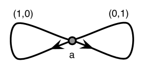
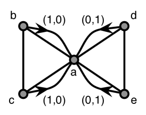
Figure 1:

Proposition 5.1.

Let $(G,\bm{\gamma})$ be as in Figure 1.(a) or Figure 1.(b). Any generic realization $G(\mathbf{p},\mathbf{L})$ is infinitesimally f.l. ultraflexible and f.l. ultrarigid.

Proof.

We begin with Figure (a). First note that for $\Psi(\gamma_{1},\gamma_{2})=\gamma_{2}\;(\text{mod}2)$, the graph $(G,\Psi(\bm{\gamma}))$ is not $\mathbb{Z}/2\mathbb{Z}$-$(2,2)$, and so generic realizations must be infinitesimally ultraflexible by Theorem 7. We fix now some arbitrary $\Lambda<\mathbb{Z}^{2}$ and prove that there are only trivial $\Lambda$-respecting motions.

Let $\tilde{G}(\mathbf{p},\mathbf{L})$ be the realization of the corresponding infinite graph $\tilde{G}$. Let $a$ be the unique vertex of $G$. Then, $\mathbf{p}_{a}(\gamma)=\mathbf{p}_{a}(0)+\mathbf{L}(\gamma)$ for all $\gamma\in\mathbb{Z}^{2}$. Let $e_{1},e_{2}$ be the standard basis vectors of $\mathbb{Z}^{2}$ and let $t_{1},t_{2}$ be the smallest positive integers satisfying $t_{i}e_{i}\in\Lambda$. Any $\Lambda$-respecting motion must necessarily preserve the difference $\mathbf{p}_{a}(t_{i}e_{i}+\gamma)-\mathbf{p}_{a}(\gamma)=\mathbf{L}(t_{i}e_{i})$ for all $\gamma\in\Gamma$. Since

$$\mathbf{p}_{a}(t_{i}e_{i}+\gamma)-\mathbf{p}_{a}(\gamma)=\sum_{k=1}^{t_{i}}(\mathbf{p}_{a}(ke_{i}+\gamma)-\mathbf{p}_{a}((k-1)e_{i}+\gamma)=\sum_{k=1}^{t_{i}}\mathbf{L}(e_{i}),$$

the sequence of vertices is “pulled tight” and so any motion must preserve the difference $\mathbf{p}_{a}(ke_{i}+\gamma)-\mathbf{p}_{a}((k-1)e_{i}+\gamma)=\mathbf{L}(e_{i})$ for $1\leq k\leq t_{i}$. This implies that the difference $\mathbf{p}_{a}(e_{i}+\gamma)-\mathbf{p}_{a}(\gamma)$ for any $\gamma,i$ is the constant vector $\mathbf{L}(e_{i})$ under any motion, i.e. all motions are trivial.

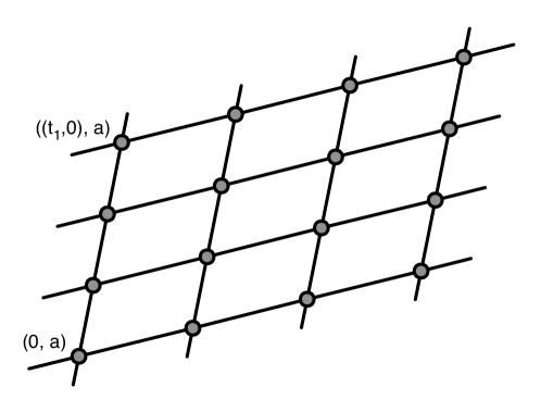
Figure 2: Periodic realization of the graph in Figure 1.(a).

Now, let $(G,\bm{\gamma})$ be the graph in figure (b). Let $\Psi$ be as above. Then, $(G,\Psi(\bm{\gamma}))$ is not $\Delta$-$(2,2)$ since the graph spanned by vertices $a,b,c$ is $(2,1)$-tight but of trivial $\Delta$ color. By Theorem 7, generic realizations are infinitesimally ultraflexible. However, as Figure 3 shows, the vertex $(a,\gamma)$ is connected to $(a,\gamma\pm e_{i})$ for $i=1,2$ by rigid graphs. Thus, as in the previous example, regardless of $\Lambda$, the orbit of $(a,\gamma)$ is pulled tight and via similar arguments the framework is rigid. ∎

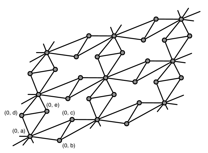
Figure 3: Periodic realization of the graph in Figure 1.(b).

In light of the above examples, we ask the following.

Problem 1.

Characterize those graphs for which infinitesimal ultraflexibility implies ultraflexibility.

5.2  Some open questions:

For many situations, infinitesimal rigidity is preserved under any sufficiently small deformation of a framework $G(\mathbf{p})$ (not necessarily preserving lengths). The reason the property holds is that infinitesimal rigidity holds outside some proper algebraic subvariety. However, the set of infinitesimally ultrarigid frameworks is, a priori, the complement of infinitely many subvarieties (one for each torsion point), and so it is unclear that the set is open.

Question 1.

For a given periodic graph, is the space of infinitesimally ultrarigid frameworks open? Does it contain any open sets?

The paper [6] provides some evidence that the answer to the latter question is yes. In [6], it is shown that periodic pointed pseudo-triangulations are f.a. infinitesimally ultrarigid and adding a single edge orbit produces an infinitesimally ultrarigid framework. Since the property of being a periodic pointed pseudo-triangulation is preserved under small perturbations, this produces open sets of ultrarigid frameworks.

On the other hand, in the context of fixed lattice ultrarigidity, Connelly–Shen–Smith have produced a continuous $1$-parameter family of frameworks where both the infinitesimally ultrarigid and ultraflexible frameworks are dense in the set of parameters. (See Theorem 9.1 of [9]. A more thorough description of the family is available in the corresponding appendix.) In this context then, the answer to the former question is, in general, negative. Moreover, it seems likely that this example can be modified to apply to the fully flexible context. Thus, one preliminary project might be to find a periodic graph where the infinitesimally ultrarigid realizations constitute an open set, if indeed such a periodic graph exists.

The results of [6], [16] and this paper lead to another natural question. In [16], it is shown that a planar Laman graph necessarily has a realization as a pointed pseudo-triangulation. As was shown in [6], $m=2n$ for a periodic pointed pseudo-triangulation, and so the frameworks must satisfy the conditions of Theorem 7.

Question 2.

If a colored graph satisfies the conditions of Theorem 7 and admits a planar periodic realization, does it admit a realization as a periodic pointed pseudo-triangulation?

Our combinatorial theorems 6 and 7 characterize generic infinitesimal ultrarigidity when the number of edges is the minimal possible. However, infinitesimal ultrarigidity is not obviously matroidal (and almost certainly not) on colored graphs. Moreover, for each torsion point $1\neq\bm{\omega}\in\mathbb{C}^{2}$, we only understand generically the rank of $\operatorname{pr}_{\bm{\omega}}(\hat{S}_{G,\mathbf{p},\mathbf{L}})$ when we assume additional combinatorial information about $(G,\bm{\gamma})$, i.e. that it is colored-Laman-sparse. Therefore, the following closely related problems remain open:

Problem 2.

In dimension $2$ (or higher), give a complete combinatorial characterization of the linear matroid given by the generic rank of $\operatorname{pr}_{\bm{\omega}}(\hat{S}_{G,\mathbf{p},\mathbf{L}})$.

Problem 3.

Characterize, without any assumption on the number of edges, the generically infinitesimally ultrarigid graphs.

References

- Aliev and Smyth [2012] I. Aliev and C. Smyth. Solving algebraic equations in roots of unity. Forum Math., 24(3):641–665, 2012. ISSN 0933-7741; 1435-5337/e. doi: 10.1515/form.2011.087.
- Berardi et al. [2011] M. Berardi, B. Heeringa, J. Malestein, and L. Theran. Rigid components in fixed-lattice and cone frameworks. In Proceedings of the Annual Canadian Conference on Computational Geometry (CCCG), 2011. URL http://www.cccg.ca/proceedings/2011/papers/paper52.pdf.
- Bombieri and Zannier [1995] E. Bombieri and U. Zannier. Algebraic points on subvarieties of . Internat. Math. Res. Notices, (7):333–347, 1995. ISSN 1073-7928. doi: 10.1155/S1073792895000250. URL http://dx.doi.org/10.1155/S1073792895000250.
- Borcea and Streinu [2012] C. Borcea and I. Streinu. Pharmacosiderite and ultrarigidity. Poster at the Royal Society workshop “Rigidity of periodic and symmetric structures in nature and engineering”, February 2012.
- Borcea and Streinu [2014] C. Borcea and I. Streinu. Liftings and stresses for planar periodic frameworks. In Proceedings of the Thirtieth Annual Symposium on Computational Geometry, SOCG’14, pages 519:519–519:528, New York, NY, USA, 2014. ACM. ISBN 978-1-4503-2594-3. doi: 10.1145/2582112.2582122. URL http://doi.acm.org/10.1145/2582112.2582122.
- Borcea and Streinu [2015] C. Borcea and I. Streinu. Liftings and stresses for planar periodic frameworks. Preprint, arXiv:1501.03549, 2015. URL http://arxiv.org/abs/1501.03549.
- Borcea and Streinu [2010] C. S. Borcea and I. Streinu. Periodic frameworks and flexibility. Proc. R. Soc. Lond. Ser. A Math. Phys. Eng. Sci., 466(2121):2633–2649, 2010. ISSN 1364-5021. doi: 10.1098/rspa.2009.0676. URL http://dx.doi.org/10.1098/rspa.2009.0676.
- Cheng et al. [2010] Q. Cheng, S. Tarasov, and M. Vyalyi. Efficient algorithms for sparse cyclotomic integer zero testing. Theory of Computing Systems, 46(1):120–142, 2010. ISSN 1432-4350. doi: 10.1007/s00224-008-9158-2. URL http://dx.doi.org/10.1007/s00224-008-9158-2.
- Connelly et al. [2014] R. Connelly, J. D. Shen, and A. D. Smith. Ball packings with periodic constraints. Discrete & Computational Geometry, 52(4):754–779, 2014. doi: 10.1007/s00454-014-9636-z. URL http://dx.doi.org/10.1007/s00454-014-9636-z.
- Dove et al. [2007] M. T. Dove, A. K. A. Pryde, V. Heine, and K. D. Hammonds. Exotic distributions of rigid unit modes in the reciprocal spaces of framework aluminosilicates. Journal of Physics: Condensed Matter, 19(27):275209, 2007. URL http://stacks.iop.org/0953-8984/19/i=27/a=275209.
- Edmonds [1965] J. Edmonds. Minimum partition of a matroid into independent subsets. J. Res. Nat. Bur. Standards Sect. B, 69B:67–72, 1965.
- Edmonds and Rota [1966] J. Edmonds and G.-C. Rota. Submodular set functions (abstract). In Waterloo Combinatorics Conference, University of Waterloo, Ontario, 1966.
- Fowler and Guest [2000] P. Fowler and S. Guest. A symmetry extension of maxwell’s rule for rigidity of frames. International Journal of Solids and Structures, 37(12):1793 – 1804, 2000. ISSN 0020-7683. doi: http://dx.doi.org/10.1016/S0020-7683(98)00326-6. URL http://www.sciencedirect.com/science/article/pii/S0020768398003266.
- Gao et al. [2000] S. Gao, J. v. Gathen, D. Panario, and V. Shoup. Algorithms for exponentiation in finite fields. Journal of Symbolic Computation, 29(6):879 – 889, 2000. ISSN 0747-7171. doi: 10.1006/jsco.1999.0309. URL http://dx.doi.org/10.1006/jsco.1999.0309.
- Giddy et al. [1993] A. P. Giddy, M. T. Dove, G. S. Pawley, and V. Heine. The determination of rigid-unit modes as potential soft modes for displacive phase transitions in framework crystal structures. Acta Crystallographica Section A, 49(5):697–703, Sep 1993. doi: 10.1107/S0108767393002545. URL http://dx.doi.org/10.1107/S0108767393002545.
- Haas et al. [2005] R. Haas, D. Orden, G. Rote, F. Santos, B. Servatius, H. Servatius, D. Souvaine, I. Streinu, and W. Whiteley. Planar minimally rigid graphs and pseudo-triangulations. Computational Geometry, 31(1–2):31 – 61, 2005. ISSN 0925-7721. URL http://www.sciencedirect.com/science/article/pii/S0925772104001063. Special Issue on the 19th Annual Symposium on Computational Geometry - SoCG 2003 19th Annual Symposium on Computational Geometry - SoCG 2003.
- Hammonds et al. [1997] K. D. Hammonds, H. Deng, V. Heine, and M. T. Dove. How floppy modes give rise to adsorption sites in zeolites. Phys. Rev. Lett., 78:3701–3704, May 1997. doi: 10.1103/PhysRevLett.78.3701. URL http://link.aps.org/doi/10.1103/PhysRevLett.78.3701.
- Hammonds et al. [1998] K. D. Hammonds, V. Heine, and M. T. Dove. Rigid-unit modes and the quantitative determination of the flexibility possessed by zeolite frameworks. The Journal of Physical Chemistry B, 102(10):1759–1767, 1998. doi: 10.1021/jp980006z. URL http://pubs.acs.org/doi/abs/10.1021/jp980006z.
- Heintz [1983] J. Heintz. Definability and fast quantifier elimination in algebraically closed fields. Theoret. Comput. Sci., 24(3):239–277, 1983. ISSN 0304-3975. doi: 10.1016/0304-3975(83)90002-6. URL http://dx.doi.org/10.1016/0304-3975(83)90002-6.
- Hindry [1988] M. Hindry. Autour d’une conjecture de Serge Lang. Invent. Math., 94(3):575–603, 1988. ISSN 0020-9910; 1432-1297/e. doi: 10.1007/BF01394276. URL http://dx.doi.org/10.1007/BF01394276.
- Kapko et al. [2011] V. Kapko, C. Dawson, I. Rivin, and M. M. J. Treacy. Density of mechanisms within the flexibility window of zeolites. Phys. Rev. Lett., 107:164304, Oct 2011. doi: 10.1103/PhysRevLett.107.164304. URL http://link.aps.org/doi/10.1103/PhysRevLett.107.164304.
- Lang [1983] S. Lang. Fundamentals of Diophantine geometry. Springer-Verlag, New York, 1983. ISBN 0-387-90837-4.
- Lee and Streinu [2008] A. Lee and I. Streinu. Pebble game algorithms and sparse graphs. Discrete Math., 308(8):1425–1437, 2008. ISSN 0012-365X. doi: 10.1016/j.disc.2007.07.104. URL http://dx.doi.org/10.1016/j.disc.2007.07.104.
- Lenstra et al. [1982] A. K. Lenstra, H. W. Lenstra, Jr., and L. Lovász. Factoring polynomials with rational coefficients. Math. Ann., 261(4):515–534, 1982. ISSN 0025-5831. doi: 10.1007/BF01457454. URL http://dx.doi.org/10.1007/BF01457454.
- Leroux [2012] L. Leroux. Computing the torsion points of a variety defined by lacunary polynomials. Math. Comp., 81(279):1587–1607, 2012. ISSN 0025-5718. doi: 10.1090/S0025-5718-2011-02548-2. URL http://dx.doi.org/10.1090/S0025-5718-2011-02548-2.
- Liardet [1974] P. Liardet. Sur une conjecture de Serge Lang. C. R. Acad. Sci. Paris Sér. A, 279:435–437, 1974.
- Malestein and Theran [2013a] J. Malestein and L. Theran. Generic combinatorial rigidity of periodic frameworks. Adv. Math., 233:291–331, 2013a. ISSN 0001-8708. doi: 10.1016/j.aim.2012.10.007. URL http://dx.doi.org/10.1016/j.aim.2012.10.007.
- Malestein and Theran [2013b] J. Malestein and L. Theran. Frameworks with forced symmetry I: reflections and rotations. Preprint, arXiv:304.0398, 2013b. URL http://arxiv.org/abs/1304.0398.
- Malestein and Theran [2014a] J. Malestein and L. Theran. Frameworks with forced symmetry II: orientation-preserving crystallographic groups. Geometriae Dedicata, 2014a. doi: 10.1007/s10711-013-9878-6. URL http://dx.doi.org/10.1007/s10711-013-9878-6. (online).
- Malestein and Theran [2014b] J. Malestein and L. Theran. Generic rigidity with forced symmetry and sparse colored graphs. In Rigidity and symmetry, volume 70 of Fields Institute Communications. 2014b. doi: 10.1007/978-1-4939-0781-6_12. URL http://arxiv.org/abs/1203.0772.
- Owen and Power [2009] J. Owen and S. Power. Continuous curves from infinite Kempe linkages. Bull. Lond. Math. Soc., 41(6):1105–1111, 2009. ISSN 0024-6093; 1469-2120/e. doi: 10.1112/blms/bdp087.
- Power [2014] S. C. Power. Polynomials for crystal frameworks and the rigid unit mode spectrum. Phil. Trans. R. Soc. A, 372(2008), Jan 2014. doi: 10.1098/rsta.2012.0030. URL http://dx.doi.org/10.1098/rsta.2012.0030.
- Ribenboim [1988] P. Ribenboim. The book of prime number records. Springer-Verlag, New York, 1988. ISBN 0-387-96573-4.
- Rivin [2006] I. Rivin. Geometric simulations - a lesson from virtual zeolites. Nature Materials, 5(12):931–932, Dec 2006. doi: 10.1038/nmat1792. URL http://dx.doi.org/10.1038/nmat1792.
- Roblot [2004] X.-F. Roblot. Polynomial factorization algorithms over number fields. Journal of Symbolic Computation, 38(5):1429–1443, 2004. ISSN 0747-7171. doi: 10.1016/j.jsc.2004.05.002. URL http://dx.doi.org/10.1016/j.jsc.2004.05.002.
- Ross [2011] E. Ross. The Rigidity of Periodic Frameworks as Graphs on a Torus. PhD thesis, York University, 2011. URL http://www.math.yorku.ca/~ejross/RossThesis.pdf.
- Sartbaeva et al. [2006] A. Sartbaeva, S. Wells, M. Treacy, and M. Thorpe. The flexibility window in zeolites. Nature Materials, Jan 2006.
- Schulze [2010a] B. Schulze. Symmetric Laman theorems for the groups and . Electron. J. Combin., 17(1):Research Paper 154, 61, 2010a. ISSN 1077-8926. URL http://www.combinatorics.org/Volume_17/Abstracts/v17i1r154.html.
- Schulze [2010b] B. Schulze. Symmetric versions of Laman’s theorem. Discrete Comput. Geom., 44(4):946–972, 2010b. ISSN 0179-5376. doi: 10.1007/s00454-009-9231-x. URL http://dx.doi.org/10.1007/s00454-009-9231-x.
- Schulze and Tanigawa [2013] B. Schulze and S.-I. Tanigawa. Infinitesimal rigidity of symmetric frameworks. Preprint, arXiv:1308.6380, 2013. URL http://arxiv.org/abs/1308.6380.
- Sun et al. [2012] K. Sun, A. Souslov, X. Mao, and T. C. Lubensky. Surface phonons, elastic response, and conformal invariance in twisted kagome lattices. Proceedings of the National Academy of Sciences, 109(31):12369–12374, 2012. doi: 10.1073/pnas.1119941109. URL http://www.pnas.org/content/109/31/12369.abstract.
- Swainson and Dove [1993] I. P. Swainson and M. T. Dove. Low-frequency floppy modes in -cristobalite. Phys. Rev. Lett., 71:193–196, Jul 1993. doi: 10.1103/PhysRevLett.71.193. URL http://link.aps.org/doi/10.1103/PhysRevLett.71.193.
- Tanigawa [2012] S.-I. Tanigawa. Matroids of gain graphs in applied discrete geometry. Preprint, arXiv:1207.3601, 2012. URL http://arxiv.org/abs/1207.3601.
- Theran [2011] L. Theran. Generic rigidity of crystallographic frameworks. Talk at the Fields Institute workshop “Rigidity and Symmetry”, October 2011. URL http://www.fields.utoronto.ca/audio/11-12/wksp_symmetry/theran/.
- Vitelli [2012] V. Vitelli. Topological soft matter: Kagome lattices with a twist. Proceedings of the National Academy of Sciences, 109(31):12266–12267, 2012. doi: 10.1073/pnas.1209950109. URL http://www.pnas.org/content/109/31/12266.short.