A multiwavelength analysis of the clumpy FIR–bright sources in M33

Abstract

We present a multiwavelength study of a sample of far-infrared (FIR) sources detected on the Herschel broad–band maps of the nearby galaxy M33. We perform source photometry on the FIR maps as well as mid-infrared (MIR), H$\alpha$, far-ultraviolet and integrated HI and CO line emission maps. By fitting MIR/FIR dust emission spectra, the source dust masses, temperatures and luminosities are inferred. The sources are classified based on their H$\alpha$ morphology (substructured versus not-substructured) and on whether they have a significant CO detection ($S/N>$3$\sigma$). We find that the sources have dust masses in the range 10²-10⁴ M_⊙ and that they present significant differences in their inferred dust/star formation/gas parameters depending on their H$\alpha$ morphology and CO detection classification. The results suggests differences in the evolutionary states or in the number of embedded HII regions between the subsamples. The source background–subtracted dust emission seems to be predominantly powered by local star formation, as indicated by a strong correlation between the dust luminosity and the dust-corrected H$\alpha$ luminosity and the fact that the extrapolated young stellar luminosity is high enough to account for the observed dust emission. Finally, we do not find a strong correlation between the dust-corrected H$\alpha$ luminosity and the dust mass of the sources, consistent with previous results on the breakdown of simple scaling relations at sub-kpc scales. However, the scatter in the relation is significantly reduced by correcting the H$\alpha$ luminosity for the age of the young stellar populations in the star–forming regions.

1 Introduction

From the morphological point of view, the dust emission observed within nearby galaxies can be roughly described in terms of a clumpy and a smoother diffuse component. At least partially, the clumpiness of the dust emission morphology is determined by the gas mass distribution: the clumpy component can be associated with massive giant molecular clouds (GMCs), with sizes of the order of $\approx 10-100$ pc, and the diffuse component with a more diffuse interstellar medium (ISM) gas, distributed on kpc scales. However, peaks of emission in the far-infrared (FIR) maps of galaxies can also be due to the presence of strong radiation sources heating the dust locally. In addition, for a given dust composition and size distribution, the diffuse dust emission spectrum will depend on the intensity and colour of the kpc scale radiation field produced by all the stellar populations in a galaxy. Therefore, the morphology of dust emission does not necessarily follow the ISM gas morphology. Understanding the intrinsic nature of the clumpy and diffuse components of dust emission is important since their spectral energy distributions carry information about both the ISM gas associated with them and the nature of the radiation sources powering them.

Multiwavelength studies of dust emission in nearby galaxies using the Herschel Space Observatory have mainly relied on pixel-by-pixel analyses (e.g. Smith et al. 2010, Galametz et al. 2012, Mentuch-Cooper et al. 2012, Foyle et al. 2012, Bendo et al. 2012). This method consists of convolving all the maps considered in the analyses to the same resolution, corresponding to the resolution of the map characterized by the largest point spread function (PSF) beam, and then comparing the emission at each wavelength or the measured dust/stellar population parameters at each pixel position. This method is advantageous for its simplicity but it has the drawback of considering simultaneously both the clumpy and the diffuse components of the dust emission. By including both components, pixel-by-pixel analyses are not in the position of distinguishing their properties.

A procedure to extract and measure the dust parameters of bright FIR compact sources within nearby galaxies has been introduced by Foyle et al. (2013, hereafter FN13) and applied to a set of multiwavelength data of the spiral galaxy M83. In order to perform the compact source photometry at the different wavelengths, FN13 used getsources, a multiwavelength source detection and photometry algorithm (Men’shchikov et al. 2012). This algorithm is designed to detect sources and extract the background–subtracted source photometry on Herschel maps in their original resolution, without degrading the maps. Thus, ideally, the highest resolution information is preserved. Furthermore, FN13 performed a two-component dust emission SED fitting to infer the dust parameters and measured star formation rates (SFR) from the dust–corrected H$\alpha$ source luminosity. This procedure provided insights on the nature of the bright FIR sources in M83 and their associated giant molecular associations (GMAs) and showed that the properties of the sources do not show radial variations, which is typically found in pixel-by-pixel studies that average over both clumpy and diffuse emission simultaneously (e.g. Foyle et al. 2012).

In this paper we apply the same procedure developed by FN13 to a set of multiwavelength maps of the nearby galaxy M33. M33 is a flocculent spiral galaxy at a distance of only 0.859 Mpc (Barker & Sarajedini 2008). Thus, it is an ideal target to study the characteristics of FIR compact sources on scales even smaller than those that can be observed in M83. The dust emission in M33 has already been the subject of several works (e.g. Tabatabaei et al. 2014, Kramer et al. 2013, Relaño et al. 2013, Xilouris et al. 2012, Boquien et al. 2011, Braine et al. 2010, Verley et al. 2010, Kramer et al. 2010). In Relaño et al. (2013; hereafter R13) they studied the dust properties of HII regions in M33 that they detected in H$\alpha$ emission. The sources were classified based on their H$\alpha$ morphology and, for each source, they measured the FIR colours and dust parameters.

We take an alternative approach to R13, by detecting sources in the FIR emission of M33 instead of H$\alpha$. At first, it might seem that these two approaches might be comparable. However, although dust in and around HII regions can be seen as a bright MIR/FIR compact source, in principle clumpy dust emission can arise also from sources not clearly detected in H$\alpha$, either because the local star formation is not intense enough for H$\alpha$ emission to be detected or because H$\alpha$ is attenuated by dust. Furthermore, a single FIR source might be related to an entire ensemble of HII regions as well as single ones.

In addition to the FIR emission, we also augment our data set with mid-infrared (MIR) and UV broad–band maps as well as H$\alpha$, HI 21cm and CO line emission maps. MIR data can be used together with the FIR measurements on the Herschel maps in order to obtain a complete MIR to FIR dust emission SED of the detected sources. Dust corrected H$\alpha$ and UV luminosities can be used to investigate star formation on different time scales, H$\alpha$ tracing more recent star formation ($10^{7}$ yr) than UV ($10^{8}$ yr). Finally, HI and CO gas maps can be used to elucidate the relation between the gas and the dust parameters.

Specifically, in this work we address the following questions:
1) What is the intrinsic nature of the bright FIR sources in M33? Are they associated with a single or with multiple HII regions? Are they mainly associated with the molecular gas detected in CO?
2) How do the dust parameters vary depending on the radial distance, the H$\alpha$ morphology, the detection of molecular gas ?
3) Is the source dust emission heated predominantly from local young stellar populations? Is there evidence of external heating?
4) Assuming that the source dust mass traces the gas mass of the cloud associated with the cospatial HII regions, is there evidence for a scaling relation between dust mass and the recent star formation within the clouds?

The paper is structured as following. Section 2 presents the data set we used. In Section 3 we describe the source extraction technique and the photometry performed at all wavelengths. Section 4 describes the dust emission SED fitting technique applied to the MIR/FIR data. In Section 5 we describe the measurements of the star formation parameters. In Section 6 we explain the criteria adopted to select our best source sample and define subsamples of sources based on their H$\alpha$ morphology and the detection of CO emission. Section 7 presents the results and in Section 8 we discuss our findings. We conclude with a brief summary.

2 Observations

As in FN13, we use FIR maps to detect and extract the photometry of compact FIR bright sources but also perform the photometry at the same source locations on MIR and H$\alpha$ emission maps. In addition, we include a far-ultraviolet (FUV) map and gas maps (CO and HI) in order to trace young stellar populations bright in the UV and the cold gas possibly associated with the FIR sources. Here we describe the data reduction prior to the source photometry. All the data used are shown in Fig.1.

2.1 FIR maps

We use FIR maps obtained by the Herschel Space Observatory. The images are part of the Herschel Open Time Key Project HerM33es (Herschel M33 Extended Survey; P.I.: C. Kramer). We use 100 and 160 $\mu$m maps taken with the Photodetector Array Camera (PACS; Poglitsch et al. 2010) and 250 and 350 maps taken with the Spectral Photometric Imaging REceiver (SPIRE; Griffin et al. 2010). The PACS and SPIRE data reduction are described in Boquien et al. (2011) and Xilouris et al. (2012) respectively. The images are kept in their native resolution with a full width at half-maximum (FWHM) of the PSF of 6.8^′′, 11.4^′′, 17.6^′′, and 24.0^′′ for the 100, 160, 250, and 350$\mu$m maps, respectively. Note that, due to the low resolution and thus high uncertainties in the source detection method, we do not include the 500$\mu$m SPIRE map in our analysis.

2.2 MIR maps

In addition to the FIR maps, we also use 8 and 24 $\mu$m maps from IRAC and MIPS instruments taken from the Spitzer Local Volume Legacy Survey (Dale et al. 2009). These MIR maps trace the warm dust and polycyclic aromatic hydrocarbon (PAH) emission. In the case of the 8 $\mu$m map, we subtract the stellar component of the emission, in order to extract only the dust/PAH emitting component. We do this by using a scaling of the IRAC 3.6 $\mu$m map, according to the relation provided by Helou et al. (2004): $F_{\nu}$(8 $\mu$m, dust) = $F_{\nu}$(8 $\mu$m)-0.232$F_{\nu}$(3.6 $\mu$m) as was done in FN13. We degrade the resolution of the MIR maps to 6.8^′′ in order to match the resolution of the 100 $\mu$m map using the kernels of Aniano et al. (2011).

2.3 FUV map

We use a FUV map from GALEX (Martin et al. 2005) and distributed by Gil de Paz et al. (2007) in order to trace UV continuum emission. Details on the image processing are found in Thilker et al. (2005). We correct Galactic extinction using E(B-V)=0.042 from the NASA/IPAC Extragalactic Database that is based on the dust extinction maps from Schlegel et al. (1998). The map is degraded from its 4.4^′′ resolution to a resolution of 6.8^′′ matching that of the 100 $\mu$m map using the kernels of Aniano et al. (2011).

2.4 H$\alpha$ map

We trace ionized gas using an H$\alpha$ emission map from Greenawalt (1998). The image and processing is described in Hoopes & Walterbos (2000). As was done for the FUV map, we correct the H$\alpha$ map for Galactic extinction. We also correct for [NII] contamination using [NII]/H$\alpha$ =0.05. We degrade the H$\alpha$ map from its 2^′′ resolution to a resolution of 6.8^′′, matching that of the 100 $\mu$m map, by using a Gaussian kernel.

2.5 Molecular gas map

In order to trace the molecular gas, we use a ¹²CO (J=1-0) map of M33 with 19.3^′′ resolution from the Nobeyama Radio Observatory (Tosaki et al. 2011). We use the moment 0 integrated intensity map, which is converted to a molecular gas mass assuming a CO-to-H₂ conversion factor of 2 $\times$ 10²⁰ cm^-2(K km s^-1)^-1 (Strong et al. 1988). We multiply by a factor of 1.36 to account for helium. We match the resolution of the map to the 350 $\mu$m map (24.0^′′) using a Gaussian kernel.

2.6 Atomic gas map

We trace the atomic gas component using HI 21 cm VLA observations (Gratier et al. 2010). The integrated intensity maps are converted to a gas mass assuming a conversion factor of 1.8$\times$10¹⁸ cm²/(K km s^-1) (Rohlfs & Wilson 1996). For consistency with the CO map, the atomic gas map is convolved from its native resolution of 17^′′ to the resolution of the 350$\mu$m map.

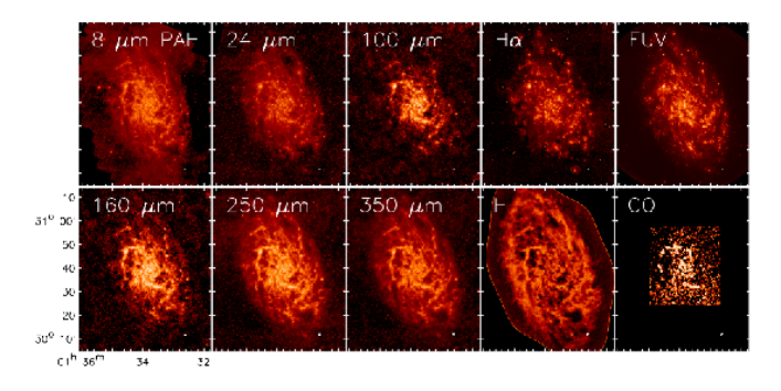
Figure 1: Multi-wavelength data used in this work. Upper row: Spitzer IRAC 8$\mu$m (stellar emission subtracted) and MIPS 24$\mu$m maps, Herschel PACS 100$\mu$m map, H$\alpha$ map from the KPNO Schmidt telescope (Greenawalt 1998), GALEX FUV map. Lower row: Herschel PACS 160 and SPIRE 250, 350 $\mu$m maps, VLA 21 cm line HI map, ¹²CO (J=1-0) integrated intensity map from the Nobeyama Radio Observatory. The diameter of the white circles at the right-bottom of each panel is equal to the PSF FWHM. Note that the resolution of the 8$\mu$m, 24$\mu$m, H$\alpha$, FUV, HI and CO maps have been degraded as described in the text.

3 Source Detection and Photometry

In this section we describe the source detection and photometry method applied to the FIR data set (§3.1) as well as the photometry performed on all the other maps at the location of the detected FIR sources (§3.2).

3.1 FIR source detection and photometry

We detect and extract the photometry of compact sources in the FIR maps using getsources, a multiwavelength and multiscale source detection tool (Men’shchikov et al. 2012). We use this tool because it can account for the different angular resolutions of the FIR maps, perform background subtractions in the vicinity of the sources and account for source blending. A description of the code and its application to the nearby galaxy M83 is provided in FN13. Here we briefly describe the main steps performed by this code.

Rather than detecting the sources in the original images, getsources creates single-scale detection maps by convolving the images with a series of gaussians and then subtracting the convolved images one from the other (see formula 1 of Men’shchikov et al. 2012). For a given spatial scale, the maps at each wavelength are combined to produce a single scale detection image. A source can then be detected and tracked through the different scales. The scale where the source is the brightest provides an initial estimate of the source size and shape. Once the sources have been detected, the original observations are used to extract the photometry of the source. A background in the vicinity of the source is also interpolated and subtracted at each wavelength.

Before the source extraction process, we first align the images to the same grid and convert them to MJy sr^-1, with a pixel size of 1.4^′′. Observational masks are made, which mark the extent of the image over which getsources searches for sources. In FN13, the MIR 24$\mu$m and H$\alpha$ maps were also included in the getsources source extraction process. However, as described below, we perform aperture photometry on the ancillary bands because, at the spatial scales observed in M33 (i.e. 28 pc at 100$\mu$m ), the emission morphology at those wavelengths may differ considerably from that observed in the FIR.

After the extraction process, getsources returns a table with the source properties including the source size, position, total flux and peak flux at each wavelength. getsources also returns a monochromatic detection significance, which is determined using the ratio of the peak flux of the source to the standard deviation in an annulus surrounding the source on the detection maps.

Since many sources are only marginally detected, we set a minimum detection significance threshold to select a sample of sources to be included in the analysis. Specifically, we required a detection significance higher than 3$\sigma$ for the 100$\mu$m and 160$\mu$m bands, which are those with the highest angular resolution in the FIR data set.

3.2 Aperture photometry at other wavelengths

After measuring the FIR fluxes for the detected sources on the Herschel maps, we perform aperture photometry at the same positions on the other maps of our data set to obtain the corresponding total fluxes. We used aperture photometry, rather than using getsources directly on the entire data set, because the morphology observed for the young stellar populations, ionized and cold gas, dust and PAH emission in the area covered by the FIR sources can be intrinsically different from the FIR morphology. For example, several close HII regions bright in H$\alpha$ might be seen as a single FIR source. The aperture sizes correspond to the source footprints inferred by getsources at 100$\mu$m for the H$\alpha$, FUV, 8 and 24$\mu$m and at 350$\mu$m for the HI and CO maps. The choice of these apertures is consistent with the angular resolutions to which we convolved the different maps.

In this way, we aim to measure the amount of H$\alpha$, UV, 8 and 24$\mu$m that presumably is physically associated with detected FIR sources. In the case of HI and CO emission, we did not seek to measure the fluxes directly associated with the FIR compact sources, since these maps present a rather smooth emission at those locations, with no or only marginal evidence of compact sources coincident with the detected FIR sources. This is partially due to the low resolution of the gas maps and partially to the fact that a large fraction of the gas could be in the form of a background component not associated with the FIR bright source. Since it was not possible to estimate a GMC mass for the FIR sources, we used the HI and CO maps only to measure gas mass column density in the areas where the sources are detected. This allows us to investigate if there is any relation between the source dust parameters and the local gas column density.

While performing the aperture photometry on the H$\alpha$, FUV, 8 and 24$\mu$m maps, we also subtracted a background emission component, which we estimated in circular apertures of different size selected by-eye throughout the galaxy disc. We also estimated the variation of the brightness in the background apertures, which was used to estimate the photometric uncertainties for each measurement. We did not apply a background subtraction for the measurements on the gas maps since our goal was to measure the total gas surface density in the region of the sources. By including a background subtraction for the FIR emission (see the previous section) and for the MIR and star formation tracers, we assume that we are removing a diffuse emission component that is not directly associated with the FIR compact source. Given the large uncertainties with any approach, we chose to apply the simple approach outlined here.

4 Dust/PAH emission SED Fitting

We fit the inferred MIR and FIR fluxes with the dust/PAH emission SED fitting procedure developed by Natale et al. (2010). As this procedure was already used in FN13, here we only summarize the method and we refer to Natale et al. (2010) and to FN13 for further details.
The observed fluxes are fit by two dust emission components: a photo-dissociation region (PDR) emission component, having a fixed spectral shape and peaking at about 70$\mu$m, and a diffuse dust/PAH emission component, representing the emission from diffuse dust heated by interstellar radiation fields (ISRF) of lower intensity compared to those powering the PDR emission. In the latter case, the spectral shape of the emission is not fixed but the best–fitting model is found within a library of 361 dust emission templates. The SED shape of these templates varies depending on the heating radiation intensity and optical/UV colour. The fitting parameters are: $\chi_{\rm UV}$, the amplitude of the UV part of the radiation field heating the diffuse dust in units of the Mathis et al. (1983) curve (representing the local ISRF); $\chi_{\rm col}$, the optical/UV ratio of the heating radiation spectra; M_SED the diffuse dust mass; F₂₄ the fraction of $24\mu$m flux due to the PDR emission template. Fig. 2 shows the SED fit for four example sources.

Apart from the fitting parameters, the SED fitting procedure also provides the diffuse dust temperature T_SED, which is the temperature of the modified blackbody with an emissivity index of $\beta$=2 reproducing the FIR bump of the best–fitting diffuse dust emission template. For comparison, we also perform standard one–component modified blackbody fits (again with $\beta=2$) to the observed SEDs by including only the FIR Herschel maps (see FN13 for details). Using this fitting technique, we infer the dust mass M_BB and temperature T_BB. Note that T_BB can sometimes be different than T_SED, because in the first case the entire flux in the FIR bands has to be reproduced by the best–fitting curve. Instead, in the two component PDR/diffuse dust SED fit, part of the flux in the FIR bands, especially at 100$\mu$m and 160$\mu$m, can be assigned to the warm PDR component. Since the relative fraction of FIR emission fit by the PDR component is higher at shorter FIR wavelengths, the T_BB temperatures are often warmer than that measured by T_SED.

5 Star formation parameters

H$\alpha$ and FUV emission fluxes need to be corrected for both Galactic extinction and internal dust attenuation. Galactic extinction is due to the Milky Way dust present in the line of sight of the observed galaxy. This is corrected using the extinction value taken from Schlegel et al. (1998), as described in §2.3 and §2.4. Internal dust attenuation is due to both the local dust close to the star–forming regions and the dust in the diffuse ISM of the observed galaxies. To correct for internal attenuation, we use empirical relations based on using the observed $24\mu$m flux as a proxy for the amount of internal attenuation. Specifically, we use the relation provided by Calzetti et al. (2007) to correct the H$\alpha$ luminosity:

$${\rm L(H}\alpha,{\rm cor)=L(H}\alpha)_{{\rm obs}}{\rm+0.031L(24}\mu\rm{m)}$$ (1)

where L(H$\alpha$)_obs and L(H$\alpha$,cor) are the observed and intrinsic H$\alpha$ luminosities respectively, while L(24$\mu$m)=$\nu$_24μm L${}_{\nu}(24\mu m)$ with L${}_{\nu}(24\mu m)$ the observed luminosity density at 24$\mu$m. Throughout the text, we will refer to the term 0.031L(24$\mu$m) as the obscured H$\alpha$ luminosity or L(H$\alpha$, obscured) and 0.031L(24$\mu$m)/L(H$\alpha$,cor) as the “fraction of obscured H$\alpha$ luminosity”.

To correct the FUV, we consider the relation D10 of Leroy et al. (2008), which can be used to calculate the SFR from the observed FUV and 24$\mu$m luminosities. We used this relation divided by 0.68$\times$10^-28, the coefficient used to convert the dust corrected FUV luminosity into SFR:

$${\rm L}_{\rm\nu,cor}{\rm(FUV)=L}_{\nu,{\rm obs}}{\rm(FUV)+3.14}\times 10^{-14}{\rm L(24}\mu\rm{m)}$$ (2)

where L_ν,obs(FUV) and L_ν(FUV) are the observed and intrinsic FUV luminosity densities.

We do not convert the H$\alpha$ and FUV luminosities into SFR, since at these spatial scales the assumptions of constant SFR and complete initial mass function (IMF) sampling are not applicable (e.g. Calzetti, Liu & Koda 2012). However, we use the dust corrected H$\alpha$ and FUV luminosities to determine a dust corrected UV-to-H$\alpha$ flux ratio. In the simple assumption of a single–age stellar population (see also Relaño & Kennicutt 2009 for a similar approach), the intrinsic UV-to-H$\alpha$ ratio can be used to derive an age for the stellar population observed within each FIR source. This is because for a single–age stellar population the H$\alpha$ luminosity fades away within 10⁷ yr while the FUV takes of the order of 10⁸ yr to disappear. The overall result is that the UV-to-H$\alpha$ ratio shows a monotonic increase as a function of the stellar population age.

To convert UV-to-H$\alpha$ ratio into stellar population ages, we considered the standard output of the software Starburst99 (Leitherer et al. (1999) for an instantaneous burst of star formation, which provides the emission spectra of a single–age stellar population as a function of age. In the calculation we assumed a Kroupa (2001) IMF, with a slope of -1.3 between 0.1 and 0.5 M_⊙ and -2.3 between 0.5 and 100 M_⊙, and solar metallicity $Z$=0.02. After extracting the UV/H$\alpha$ ratio as a function of age from the Starburst99 output, we use this theoretical relation to convert the observed UV/H$\alpha$ ratio of each source into an age. Then, we use this information to correct the source H$\alpha$ luminosity for age effects. That is, we derive the H$\alpha$ luminosity that each source would have had if they all were $t$=6$\times 10^{6}$  yr old and call this age-corrected H$\alpha$ luminosity L(H$\alpha$,age). To this purpose, the correction one needs to multiply by the observed dust corrected H$\alpha$ luminosity is equal to L(H$\alpha$,$t_{o}$)/L(H$\alpha$,$t_{s}$), where L(H$\alpha$,$t$) are the H$\alpha$ luminosities calculated by the Starburst99 run at time $t_{o}$=6$\times$10⁶ yr and at the source age $t_{s}$. As discussed in Section §7.4, the age corrected H$\alpha$ luminosity allows a fairer comparison between the sources when discussing the star formation associated with them.

The above procedure which is used to determine an age-corrected H$\alpha$ luminosity is not free of caveats. First, while the H$\alpha$ correction using the Calzetti et al. (2007) formula has been calibrated also on spatial scales similar to those analysed in this work, the FUV dust correction formula from Leroy et al. (2008) has been calibrated on slightly larger scales of the order of $\approx 1$kpc. Also, the assumption of single–age stellar population is not completely correct. For example, in the cases where more H$\alpha$ sources are seen within a single FIR aperture (see the next section), it is probable that the observed stellar populations are not born exactly during the same star formation event. A more accurate analysis could be done by using multiwavelength data of the stellar emission for the young star clusters in M33 in order to derive the star formation history from spectral SED fitting (see Sharma et al. 2011). However, this kind of analysis is beyond the scope of this paper.

6 Source Selection and Classification

getsources detects 600 sources in the FIR maps. However, for our analysis we select only the sources well-detected in the FIR bands with highest angular resolution. That is, we consider only the detected sources having a monochromatic detection significance at 100$\mu$m and 160$\mu$m higher than 3$\sigma$. This reduces the sample to 348 sources. We also make another cut to the source list by selecting only those having a minimum $\chi^{2}$ in the dust emission SED fitting lower than 10 (228 sources left). Finally, we consider only the sources in the field of view common to all the maps. This leaves us with 183 well-detected sources with reasonably good SED fits and with photometry at all wavelengths.

It is important to note that the sources rejected due to our detection significance criteria and $\chi^{2}$ cut are not located preferentially in particular regions within the galaxy. There are number of reasons which may cause a source to have a low detection significance: 1) the source may be intrinsically faint and/or in a region with high background noise, 2) the source may be in a crowded region where deblending is more uncertain and 3) spurious sources may be detected by getsources due to large emission enhancements. On the other hand the sources which we discarded because of the low quality of the SED fit ($\chi^{2}$ cut) typically have one or two data points which make the entire SED quite irregular. This probably reflects difficulties in the extraction/photometry for those sources, especially for crowded regions and at longer wavelengths where deblending is more problematic.

In order to elucidate the effects on the dust parameters related to the characteristics of the young stellar populations and the cold gas, observed at the same positions of the FIR sources, we subdivide our best source sample into sub-categories. After a visual inspection of the multiwavelength emission in the regions of each source, we differentiate the sources based on their H$\alpha$ morphology and the amount of or lack of CO emission. By visually examining the H$\alpha$ emission within each FIR source footprint on the unconvolved H$\alpha$ map, we classify the sources as non-substructured (NOSUB) or substructured (SUB). NOSUB sources are characterized by a single peak in H$\alpha$ while SUB sources show a more complex morphology, characterized by multiple peaks or an irregular smoother emission. In physical terms, the difference in morphology might depend on whether the FIR source is associated with a single or with multiple HII regions. The upper two panels of Fig. 3 show the location of the NOSUB and SUB sources. Examples of NOSUB and SUB sources are shown in the upper two rows of Fig.2.

The visual inspection of the multiwavelength data also led us to differentiate between sources which are well-detected or not in CO, which we label “HighCO” and “LowCO”. Specifically, a source is classified as HighCO if, within the FIR source footprint, there is a detection in the molecular gas map that exceeds three times the rms noise level in the map (that is, if there is at least a position where the molecular gas column density is higher than 3$\times$10 M_⊙pc^-2). In the opposite case, the source is classified as LowCO. The lower two panels of Fig. 3 shows the location of HighCO and LowCO sources. The lower two rows of Fig.2 show examples of a HighCO and LowCO source.

The number of sources in each group can be found in Table 1. Note that each detected source has two labels, one for each type of source classification. For example a given source might be simultaneously a NOSUB and HighCO source. Hereafter, the total source sample will be referred as “ALL” sample. In Table 2 we provide a list of the properties inferred for each source based on the SED fitting, modified blackbody fitting, aperture photometry and corrected H$\alpha$ and UV luminosities. The measured fluxes in each band, the results of the two component SED fitting and the classification labels for the sources belonging to our best sample can be found in the appendix.

Table 1: Source classification

Name	Description	Number
NOSUB	single H$\alpha$ source	125
SUB	substructured in H$\alpha$	58
HighCO	well detected in the molecular gas map (S/N $>$ 3$\sigma$)	73
LowCO	not or only marginally detected in the molecular gas map (S/N $<$ 3$\sigma$)	110

Table 2: Inferred source properties

Label	Description
SED fitting parameters
MSED	total dust mass of the source inferred from the two–component SED fit
TSED	cold dust temperature of the source inferred from the two–component SED fit
TBB	dust temperature of the source inferred from a modified blackbody fit of the FIR bands with $\beta$=2
LTOT	total dust luminosity inferred from the two-component SED fit
LPDR/LTOT	fraction of total dust luminosity attributed to the PDR component
Star formation parameters
L(H$\alpha$,cor)	H$\alpha$ luminosity corrected for dust attenuation
L(H$\alpha$,obscured)/L(H$\alpha$,cor)	fraction of dust obscured H$\alpha$ luminosity
L(FUV, cor)/L(H$\alpha$,cor)	ratio of the dust–corrected UV luminosity to the dust–corrected H$\alpha$ luminosity
L(H$\alpha$,age)	H$\alpha$ luminosity corrected for dust attenuation and age effects
$\Sigma_{\rm gas}$	local total gas (HI $+$ H2) column density in the vicinity of the source

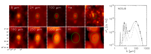
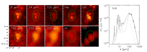
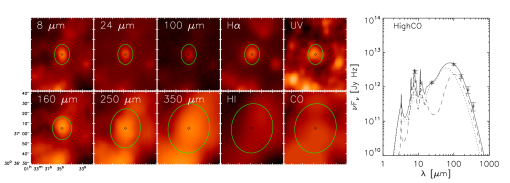
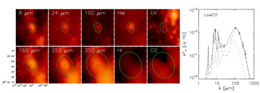
Figure 2: Example of NOSUB (top), SUB (second from top), HighCO (second from bottom) and LowCO (bottom) sources detected on the FIR Herschel maps. The left–hand panels show the emission at each wavelength, delimited by the elliptical green contours (semi-axis equal to FWHM), and the right–hand plot show the observed source dust emission SED fit by using the PDR (dotted) and diffuse dust (dashed) emission components.

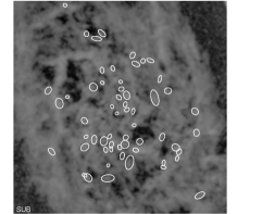
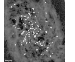
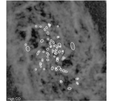
Figure 3: Source footprints at 160$\mu$m overplotted on the inner regions of the HI map with CO coverage (see bottom right–hand panel of Fig 1 for extent).

7 Results

In this section we present the results we obtained from our analysis. In §7.1 we show the distributions of the inferred dust and star formation parameters for the entire source sample and the different source categories. In §7.2 we show how these parameters vary with radial distance. In §7.3 we show the results concerning the dust heating in the FIR sources and in §7.4 those related to the star formation and gas associated with them.

7.1 Inferred Properties of Complete Sample and Subsamples

In order to show the distributions of inferred parameters and compare them for the different subsamples of compact sources, we created box-and-whisker plots which are shown in the panels of Fig. 4. The solid line in the centre of the boxes shows the median value and the box delineates the 25th and 75th quartiles. The lines extend to either the maximum and minimum values or to 1.5 times the 75th and 25th quartiles. If there are values beyond the later range, they are denoted with open circles.

We first consider the general properties of the entire sample (labelled ‘ALL’ in the box-whisker-plots). In general, we find that the compact sources have dust masses between 10²-10⁴ M_⊙ and a median value of 1890 M_⊙ (panel A). This implies gas masses of approximately 10⁴-10⁶M_⊙ assuming a constant gas-to-dust ratio of the order of 100. Due to the proximity and superior spatial resolution of M33, the compact sources are an order of magnitude smaller than that detected in M83 (FN13), with median radii of 60 pc at 100$\mu$m resolution. Thus, these compact sources likely represent a combination of GMCs and larger giant molecular associations (GMAs).

In panels B and C of Fig. 4 we show the dust temperatures inferred from the two component SED fitting procedure (T_SED) and the one–component modified blackbody fit (T_BB). The temperatures both fall in the range of 15-35 K. The T_SED temperatures tend to be lower (median value of 20 K) in comparison to T_BB temperatures (median value of 24 K). Differences between the two temperatures are expected because of the different way to fit the SEDs, with one or two components (see also §4).

The compact sources have dust luminosities of $\approx$10³⁹-10⁴⁰ erg s^-1 (panel D). We note that there are no sources fainter than 10^38.5 erg s^-1 in our sample. However, some of the fainter sources detected by getsources are excluded because of the assumed lower limit for the S/N ratio (see §6). In general, the diffuse component of the SED fit dominates the total luminosity and we find a median value of the PDR-to-total dust luminosity ratio of 0.32 (panel E).

The compact regions have dust-corrected H$\alpha$ luminosities in the range of 10^36.5-10^38.5 erg s^-1 (panel F). The sources have a median FUV-to-H$\alpha$ luminosity ratio of 2.1 (panel G) and the fraction of obscured H$\alpha$ luminosity has a median value of 0.25 (panel H). The median total gas column density within the source areas is 15 M_⊙ pc^-2 (panel I).

Looking at Fig. 4, we find that there are differences between source subsamples. We examine to what extent the properties of the sources in the SUB-NOSUB and HighCO-LowCO subsamples have similar distributions, by employing a two-sided Kolmogorov–Smirnov test (hereafter KS-test). Following Hughes et al. (2013), we take each property and repeat the KS-test 500 times sampling the property within 3$\sigma$ of the uncertainties. The median $p$-values are calculated for each test and listed in Table 3. We consider two distribution statistically different when $p<$ 0.05, which is a 95% confidence interval. We find that the samples do show some statistically significant differences. We first compare the compact sources that show substructure in H$\alpha$ (SUB sample) to those sources that only show a single peak in H$\alpha$ (NOSUB sample).

By performing KS-tests of the NOSUB and SUB subsamples we find that the sub-samples show different PDR-to-total dust luminosity ratio and FUV-to-H$\alpha$ luminosity ratios. The SUB sources have lower fractions of PDR-to-total dust luminosity with median values of 0.26 in comparison to 0.36 for the NOSUB sources. The SUB sources have a median FUV-to-H$\alpha$ luminosity ratio that is 1.5 times higher than that of the NOSUB sources. The SUB sources also have much greater extents with areas that are close to three times greater than that of the NOSUB sources (see panel J of Fig. 4 ).

The differences between NOSUB and SUB sources point to a scenario wherein the SUB sources are larger sources, containing a higher fraction of diffuse cold dust, as shown by their lower L_PDR/L_TOT ratio. They also tend to be associated with a higher fraction of more evolved UV emitting stars, as shown by their higher FUV-to-H$\alpha$ luminosity ratios compared to the NOSUB sample. In contrast, the single peak sources of the NOSUB sample are likely more isolated young star–forming regions.

Next we compare the subsamples of sources that either demonstrate a molecular gas detection (as traced by CO), with a signal-to-noise ratio higher than three times the rms-noise level, or demonstrate less significant or no detection. As defined in Section §6, we refer to these subsamples as HighCO and LowCO respectively. A similar KS-test shows that the two subsamples present different distributions for the dust temperature, total dust luminosity, the dust-corrected H$\alpha$ luminosity, the fraction of obscured H$\alpha$ luminosity and the gas column density.

The HighCO sample has warmer dust temperatures (median values of 22.3 K) than the LowCO sample (median values of 18.8 K). Since the masses of both samples are comparable, this translates into higher dust luminosities for the HighCO sample (median dust luminosity of 4.0 $\times$ 10³⁹ erg s^-1) and lower dust luminosities for the LowCO sample (median value of 1.6 $\times$ 10³⁹ erg s^-1). We also note that the HighCO sample show higher dust-corrected H$\alpha$ luminosities with median values twice as high as the LowCO sample. The relative amount of obscured H$\alpha$ luminosity to total dust H$\alpha$ luminosity is higher for the HighCO sample with a median value of 0.3 in comparison to a median value 0.2 for the LowCO sample. As expected, the HighCO samples show higher gas column densities with a median value of 24 M_⊙ pc^-2 in comparison to 12 M_⊙ pc^-2 for the LowCO sample.

The differences seen between the HighCO and the LowCO sample suggest that the HighCO sample is characterized by a higher star formation activity. This is suggested by the higher H$\alpha$ dust-corrected luminosity in the HighCO sample, while the distribution of dust mass is quite similar to that of the LowCO sample. The star formation in the HighCO sample is also plausibly producing a stronger radiation field, which leads the dust temperature and the dust luminosity to higher values than the LowCO sample. This is to be expected given that star formation is tightly coupled to molecular gas (i.e. Bigiel et al. 2008).

Finally, we note that whether the sources display a HighCO or LowCO detection show no obvious relation to the H$\alpha$ morphology. About 68% of the entire source sample is classified as NOSUB. Within the HighCO sample, 73% of the sources are from the NOSUB sample, while the fraction reduces to 62% in the LowCO sample. Thus, the NOSUB sources are only slightly more represented in the HighCO sample and slightly underrepresented in the LowCO sample.

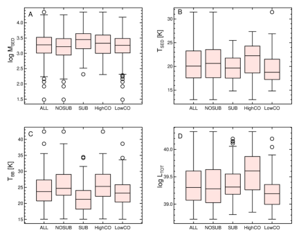
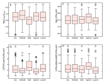
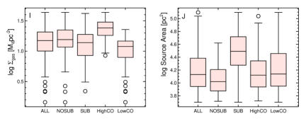
Figure 4: Box-and-whisker plots for the measured source parameters. (a) Dust mass, (b) two component SED fit temperature T_SED, (c) modified blackbody dust temperature T_BB, (d) Dust luminosity, (e) PDR–to–total dust emission luminosity ratio, (f) dust corrected H$\alpha$ luminosity, (g) dust corrected FUV to H$\alpha$ luminosity ratio, (h) obscured to total H$\alpha$ luminosity ratio, (i) total gas mass surface density within the 350$\mu$m source footprint, (j) deprojected source footprint area at 100$\mu$m

Table 3: $p$-values from KS-tests

Property	SUB-NOSUB	HighCO-LowCO
TSED	0.24	$<$ 0.01
MSED	0.076	0.39
LTOT	0.10	$<$0.01
L(H$\alpha$, cor)	0.54	$<$0.01
L(FUV,cor)/ L(H$\alpha$, cor)	0.016	0.32
L${}_{\rm PDR}/$LTOT	0.013	0.62
L(H$\alpha$, obscured)/L(H$\alpha$, cor)	0.20	$<$0.01
$\Sigma_{\rm gas}$	0.48	$<$0.01

7.2 Radial Trends

In Fig. 5 we examine how the inferred properties of the FIR detected sources in M33 vary with radius. We assume an inclination of 56^o and a position angle of 23^o (Corbelli & Schneider 1997) in order to determine the deprojected radial position. We show the values for the entire sample (grey points) and also show the median values in radial bins of 1 kpc width for the four different subsamples.

We find that, in general, the properties of the compact sources do not show strong radial dependencies (see the Spearman rank correlation coefficients in top right of each panel), although some parameters present mild or weak radial trends. While the source dust mass do not vary much with radius (panel A), the dust temperature of the sources, as measured by the two–component SED fit, decreases with radius and is on average 20% higher inside 2 kpc (panel B). Interestingly, the dust temperature inferred by the single component modified blackbody fit (panel C) does not show a radial variation¹. We also find that the dust luminosity shows a mild negative trend with radius (panel D) and is, on average, at least a factor of two greater within 2 kpc compared to larger radii. The PDR–to–total dust luminosity ratio presents only a very weak positive trend with radius (panel E). A modest declining trend is shown by both the dust corrected H$\alpha$ luminosity (panel F) and the fraction of obscured H$\alpha$ luminosity (panel H, see also Sect. 7.3.2 for discussion on this result). Instead the FUV–to–H$\alpha$ luminosity ratio shows only a weak increase with radius (panel G).

Unlike the source dust mass, the gas column density in the regions associated with the sources shows a small decline with radius, with sources in the inner 2 kpc having a column density 25% higher (panel I). We note that LowCO sources are mainly found at radii higher than 1 kpc while HighCO sources are rare beyond 3 kpc. Therefore, the radial trend shown by the gas column density for the entire sample probably reflects the radial decline of the fraction of sources well–detected in CO (note also that, taken individually, both LowCO and HighCO sources seem actually to show an increasing radial trend in panel I). Finally, the relative fraction of molecular gas for the HighCO subsample appears to decrease with radius, with the sources within the inner 2 kpc having more than double molecular gas fraction than the sources at larger radii (panel J). We note, however, that a negative metallicity radial gradient in the galaxy would act to increase the amount of molecular gas relative to the measured CO flux for the sources at larger radii (Galametz et al. 2011). However, recent studies have shown that the metallicity gradient in M33 is shallow, with a central abundance of 12 + log(O/H) =8.36 and a gradient of -0.027 dex kpc^-1 (Rosolowsky & Simon 2008).

The change in molecular gas fraction could be linked to the other observed trends, namely for the dust luminosity and the diffuse dust temperature as well as the weaker trends for the H$\alpha$ luminosity and the fraction of obscured H$\alpha$ luminosity. All these trends are consistent with the sources presenting a higher amount of star formation at shorter radii as well as being more opaque to the radiation emitted by the local young stellar populations. Further insights on the relation between local star formation and dust heating in the sources will be given in the next section.

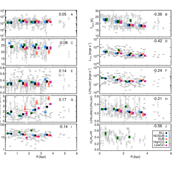
Figure 5: Source parameters plotted versus deprojected radial distance. (a) Dust mass; (b) two component SED fit temperature T_SED, (c) modified blackbody dust temperature T_BB, (d) total dust luminosity, (e) PDR–to–total dust emission luminosity ratio, (f) dust corrected H$\alpha$ luminosity, (g) dust corrected FUV to H$\alpha$ luminosity ratio, (h) obscured to total H$\alpha$ luminosity ratio, (i) total gas mass surface density within the 350$\mu$m source footprint, (j) fraction of molecular gas (only for HighCO sources). Each source is displayed in grey and the Spearman rank correlation coefficient for the entire sample is listed in the upper right. The median values in bins of 1 kpc are displayed in colour according to the legend in panel (j) and are slightly offset for visual clarity. The uncertainties on the coloured points reflect median uncertainties.

7.3 Dust heating within the FIR sources

7.3.1 Dust luminosity and H$\alpha$ luminosity

The complete source sample as well as all the subsamples show a strong correlation between the total dust luminosity L_TOT and the dust corrected H$\alpha$ luminosity L(H$\alpha$,cor) (see Fig.6). As discussed in FN13, the presence of this correlation is expected if the dust luminosity is predominantly heated by the local young stellar populations provided one can assume that the luminosity-weighted optical depth $\tau$ (integrated over wavelength) is similar for all the sources. Interestingly, for a given H$\alpha$ luminosity, the LowCO sources have dust luminosities which are systematically lower than the HighCO sources. This could be another indication that the HighCO sources are more obscured star formation regions, which are expected to be more opaque and thus absorbing radiation from the embedded young stars more efficiently. Fig.6 shows no clear differences between the SUB and NOSUB sources. However, the SUB sources are confined to a narrower range of values than the NOSUB sources. We note that in Fig.6 median values are not plotted if there are less than 10 sources in a bin.

If one assumes a continuous star formation history for the FIR detected sources, one can derive the amount of total luminosity emitted by the cospatial young stellar populations for a given H$\alpha$ luminosity. To this purpose, we consider the SFR-L_dust relation from Calzetti (2012), which assumes the IMF from Kroupa et al. (2001) and solar metallicity:

$${\rm SFR[M}_{\odot}{\rm/yr]=2.8}\times 10^{-44}{\rm L}_{\rm dust}{\rm[erg/s].}$$ (3)

In this equation, L_dust coincides with the total young stellar luminosity while the SFR can be considered in this case directly proportional to the H$\alpha$ luminosity, that is, SFR[M_⊙/yr]=5.3$\times$10^-42L(H$\alpha$,cor)[erg/s] (Calzetti et al. 2007). By combining the two previous relations, one can obtain the total young stellar luminosity as a function of L(H$\alpha$,cor). This relation is plotted in Fig.6 as a solid line and denotes the maximum dust luminosity that can be powered by the local young stellar populations assuming a constant SFR. We notice that the line lies well above the inferred source dust luminosities for the M33 sources for each value of L(H$\alpha$,cor). This shows that the total intrinsic luminosity of the young stellar populations is more than sufficient to power the observed dust emission in the assumption of a constant SFR.

One can also compare the observed data with the theoretical prediction for the total young stellar luminosity in the case of an instantaneous burst of star formation (that is, a single–age stellar population). In this case the ratio between the bolometric stellar luminosity and the H$\alpha$ luminosity is not constant but increases with time (since the H$\alpha$ emission fades away quicker than the stellar luminosity). We used Starburst99 to derive the predicted ratio of the total stellar luminosity to the H$\alpha$ luminosity for an instantaneous burst of star formation as a function of time. In this calculation we assume the standard input parameters of Starburst99 including the same IMF and metallicity as before. The dashed lines in Fig.6 represent the total stellar luminosity of a young stellar population for each value of H$\alpha$ at times $t$=10⁴ yr and $t$=4$\times$10⁶ yr from the initial event of star formation. Similarly as before, these lines denote the maximum dust luminosity that can be powered by the local young stellar populations at the two selected ages. We note that most of the observed points in M33 lie between these two curves. This means that, assuming that the star formation regions are older than few $10^{6}$ yr, the amount of total stellar luminosity is enough to power the observed dust emission in this case as well. Thus, with reasonable assumptions on the star formation history for these sources, it seems that the young stellar population luminosity is sufficient to account for the entire dust emission.

This finding can be compared with the analogous result we obtained in FN13 for the FIR bright sources in M83. In FN13, however, we found evidence for extra–heating in addition to that provided by the local young stellar populations. For ease of comparison, we plot the sources detected in M83 in Fig.6, using the so called “High background measurements” in that paper. From this figure, one can see that the sources in M83 are more luminous in both dust and H$\alpha$ emission. This is likely due to the fact that the spatial resolution in M83 is lower (130  pc at 70$\mu$m versus 28  pc at 100$\mu$m for M33). Thus, the detected compact sources are more massive and presumably contain multiple embedded star–forming regions. However, more importantly, it is also evident that the L_TOT-L(H$\alpha$,cor) ratio for the M83 sample is higher than that observed for the M33 sample. This is seen by comparing the position of the points for the two source samples with the line corresponding to a constant SFR. As suggested in FN13, additional heating from the local old stellar populations or the diffuse ISRF of the galaxy may boost the dust luminosity close to or above the constant SFR line. This additional dust heating for the M83 sources could approximately compensate the fraction of young stellar luminosity escaping unabsorbed from each source. In M33, however, the heating from local young stellar populations seems enough to account for the entire dust emission. We note that the higher dust to H$\alpha$ luminosity ratio for the M83 sources might also be related to the different spatial resolution of two studies. As a consequence, the sources detected in M83 might contain a larger fraction of cold dust, plausibly located in between the multiple star formation regions within each FIR source. This dust component might be heated significantly by older or non-local stellar population apart from the local young stars.

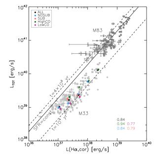
Figure 6: Dust luminosity versus H$\alpha$ line luminosity for the FIR detected sources in M33 (this work) and in M83 (see FN13). The continuous line represents the total stellar population luminosity for a given amount of H$\alpha$ luminosity in the case of a constant SFR. The dashed lines correspond to the stellar luminosity in the case of a single–age stellar population with ages $t=10^{4}$ yr and $t=10^{6}$ yr. The median values of the sources within bins of size 0.32 dex are displayed using the same colour scheme as Fig. 5. The correlation coefficient between the dust and H$\alpha$ luminosity is listed for each sample in the bottom right.

7.3.2 Dust-to-H$\alpha$ luminosity ratio versus radial distance

We also examine whether the ISRF due to the total stellar population of M33 is a significant source of dust heating, powering at least a fraction of the dust emission from the compact sources. This can be the case if the molecular clouds associated with the FIR sources are also heated externally by the galactic ISRF. To do so we plot the ratio of the dust-to-H$\alpha$ luminosity versus the deprojected radial distance. In fact, if both the ISRF and local star formation play a significant role in heating the dust, the source dust-to-H$\alpha$ luminosity ratio can be written as:

$$\frac{L_{\rm TOT}}{L(\rm{H\alpha,cor})}=\frac{L_{\rm TOT}^{\rm ISRF}(r)}{L(\rm{H\alpha,cor})}+\frac{L_{\rm TOT}^{\rm loc}}{L(\rm{H\alpha,cor})}$$ (4)

where L${}_{\rm TOT}^{\rm ISRF}$ is the dust luminosity powered by the galaxy ISRF and L${}_{\rm TOT}^{\rm loc}$ is the dust luminosity due to the absorption of local young stellar luminosity. We expect this ratio to decline with radius if 1) L${}_{\rm TOT}^{\rm ISRF}$ is not negligible and declines with radius following the decline of the galaxy interstellar radiation field; 2) the H$\alpha$ luminosity does not vary systematically with radius or it varies differently than L${}_{\rm TOT}^{\rm ISRF}$; 3) the ratio L${}_{\rm TOT}^{\rm loc}$/L(H$\alpha$,cor), proportional to the source local opacity, is on average similar at all radii. As shown in Fig.7, there is at most only a modest declining trend for this ratio with radial distance (the Spearman’s rank correlation coefficient for the entire sample is equal to -0.19). This result is consistent with only a small fraction of the total dust emission heated by the galaxy ISRF. However, as shown in Sect. 7.2, the absorbed fraction of H$\alpha$ luminosity shows a small decline with radius. One might expect this quantity to be at least roughly proportional to L${}_{\rm TOT}^{\rm loc}$/L(H$\alpha$,cor). Therefore, it might be that the small radial trend observed for $L_{\rm TOT}/L(\rm{H\alpha,cor})$ is due to the fact that, although the sources are heated predominantly by the local star formation, at shorter radii they are simply obscuring more efficiently the radiation from the local young stellar populations. If this is the case, the term $L_{\rm TOT}^{\rm ISRF}(r)$ would not actually be needed to justify the observed small radial trend for $L_{\rm TOT}/L(\rm{H\alpha,cor})$. This interpretation is consistent with a negligible contribution from the galaxy ISRF to the compact source dust heating.

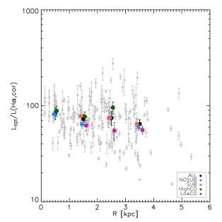
Figure 7: Ratio of the dust luminosity to the H$\alpha$ luminosity versus the deprojected radial distance for the full sample (grey points). Median values in bins of 1 kpc size are shown for each subsample.

7.3.3 Dust mass – dust temperature anticorrelation

An anticorrelation between dust mass and dust temperature has been observed by FN13 for the sample of FIR compact sources in M83. FN13 suggested that the lack of points in the lower left part of the dust mass - dust temperature plot was due to the lower limit for the dust luminosity of the sources detectable on the FIR maps of M83. For M33 we find a similar effect. Plotting the dust mass versus dust temperature for the entire source sample (see Fig.8), we find that there is an anticorrelation between the two parameters which is also present for the single subsamples separately. This result is reminiscent of the dust temperature–dust spectral index (T-$\beta$) anticorrelation found when fitting modified blackbody curves to FIR data of nearby galaxies (e.g. Galametz et al. 2012). While the T-$\beta$ anticorrelation may be due to an intrinsic variation of dust properties in the ISM of galaxies, it is also possible that this anticorrelation is due to the effect of data noise combined with the intrinsic degeneracy of the T and $\beta$ parameters in determining the spectral shape of emission within limited wavelength ranges (see Shetty et al. 2009).

However, at variance with the T and $\beta$ anticorrelation, there is no intrinsic degeneracy between T_SED and M_SED, which would produce similar spectral shapes for different pairs of these parameters and thus contribute to the observed anticorrelation between these two. While a higher value of T_SED requires a lower M_SED to fit a certain monochromatic flux, we note that the spectral shape of the templates used in the source SED fit is affected only by T_SED but not by M_SED, which is only a scaling factor.

Instead, as in the case of M83, there are several indications that the observed trend is mostly due to the lower limit of the observed dust luminosity for the well-detected sources. In order to show this, we plot in Fig. 8 a curve such that $M_{{\rm dust}}T^{6}_{{\rm dust}}$ is constant. The points belonging to this curve represent the $M_{{\rm dust}}$ and $T_{{\rm dust}}$ combinations which give the same total luminosity for a modified blackbody spectra $k_{\lambda}B_{\lambda}(T_{{\rm dust}}$) with $k_{\lambda}\propto\lambda^{-2}$. Specifically, the corresponding luminosity for the plotted curve is $\approx 8\times 10^{38}$ erg/s and we note that the curve is roughly consistent with the lower boundary for the region occupied by the measurements². However, this lower limit for the dust luminosity is determined by how well the fluxes in the single infrared wavebands are measured. That is, if the lower boundary in the M_SED–T_SED plane is due to the flux detection limits, one should find that, for a given combination of M_SED and T_SED below the curve, the predicted monochromatic fluxes are below the detection thresholds. We checked this by predicting the observed fluxes in the FIR, using our theoretical diffuse dust emission templates used in the two component SED fitting procedure, assuming combinations of dust mass and temperature in that area. The predicted fluxes are either well below or, for combinations of dust mass and temperature close to the solid curve in Fig.8, just comparable with those of the faintest sources we detected with getsources (after the removal of sources with low detection significance, see §6). For example for T_SED=20 K and M_SED=4$\times$10² M_⊙ (just below the plotted line), the predicted 100$\mu m$ flux is about 0.08 Jy which is at the lower end of the flux distribution of our source sample.

We also note a rather scarcity of sources in the upper right part of the M_SED-T_SED diagram. The lack of a homogeneously distributed high mass–high temperature sources could be due to physical effects at variance with the lack of sources in the lower left part of the diagram. Alternatively, more massive clouds might simply appear fragmented when observed in dust emission, and thus detected as multiple less massive sources.

When we consider the median trends for the different samples separately, there are no particular differences except the fact that the LowCO sources have systematically lower median dust masses compared to the HighCO ones for a given dust temperature.

We conclude that the observed anticorrelation is mainly due to the lower limit in source luminosity in our sample, causing the lower boundary of the region where the sources are confined, and perhaps a different physical (or observational) effect could be responsible for determining a lower density of points in the upper-right part of the diagram. It is important to take into account the existence of this correlation when quantities depending on dust mass and temperature are plotted versus each other. Observed correlations might be misinterpreted if one overlooks the relation between these two parameters.

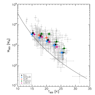
Figure 8: Inferred dust mass versus dust temperature from the MIR/FIR SED fit for the entire sample (grey points). We show median values within bins of size 2.6 K for each of the subsamples. The plotted curve pass through points of same modified blackbody luminosity (see the text for details).

7.4 Gas column densities, GMC dust masses and star formation

We now examine how the source dust masses compare to the local gas column densities in that region. We make note here that the average column density of the gas has been measured using aperture photometry with fairly large apertures that scale with the size of the source at 350$\mu$m. In contrast, the source dust mass has been determined by extracting the bright FIR sources and subtracting the background emission. While dust is generally well-mixed with gas, we would not necessarily anticipate that the mass of the clumpy source would scale with average column density in a given region. In Fig. 9 we plot the local average column density of the gas versus the dust mass of the clumpy sources. In general, we do not find a strong correlation between the source dust mass and the average gas column density. In addition to the total gas column density we also consider the gas phases and plot the molecular gas column density (HighCO sources only) and the atomic gas column density for all sources. The different gas phases also do not show evident correlations. This suggests that a wide range of inferred GMC masses can be found in regions of similar gas density (averaged over  100pc).

We also examine how the total dust-corrected H$\alpha$ luminosity scales with source mass (left-hand panel of Fig. 10). If we assume that the dust traces gas and that the dust-corrected H$\alpha$ luminosity is tracing recent star formation, this plot is equivalent to plotting the total star formation rate versus the gas mass of the GMCs associated with the FIR sources³.

On large scales it is well-known that the star formation rate per unit area is well-correlated to the gas column density (Kennicutt–Schmidt relation; Kennicutt 1989). While Fig. 10 is similar there are important differences: 1) we are plotting total values instead of surface brightnesses; 2) the source sizes are much smaller than the typical regions used to recover such a relation. Indeed, we do not recover a strong correlation between the mass of the GMCs and the dust-corrected H$\alpha$ luminosity. This is not surprising particularly given the scales we are probing (see e.g. Onodera et al. 2010 and Schruba et al. 2010).

One of the plausible reasons for the breakdown of the correlation is the spread in ages of the young stellar populations associated with the different clouds, which causes the intrinsic H$\alpha$ luminosity to vary given the same amount of young stellar mass. Therefore, one might expect that if we can correct the H$\alpha$ luminosity for the stellar population age, we could recover the relation or at least reduce the observed scatter. We attempt to do this in the right-hand panel of Fig. 10. Here we plot the dust-corrected H$\alpha$ luminosity that has been corrected for the source age, assuming that each source can be modelled by an instantaneous starburst, as described in §5. We find that the correlation coefficients increase and that the scatter is reduced. This result suggests that the spread in ages of the stellar populations in the different sources is indeed one of the important factors determining the breakdown of observed star formation relations at the scales of GMCs. These results will be further discussed in Sect. 8.2.

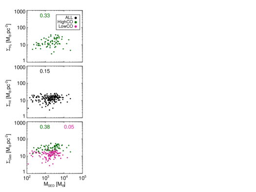
Figure 9: Molecular, atomic and total gas mass surface density versus source dust mass. The correlation coefficients are shown at the top of each panel according to the coding in the legend.

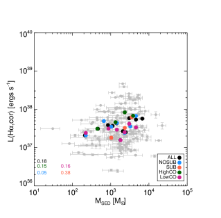
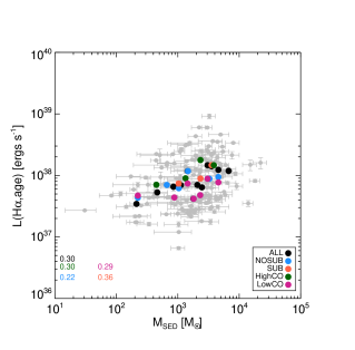
Figure 10: Source dust-corrected H$\alpha$ luminosity versus dust mass (left) and H$\alpha$ luminosity corrected for both dust attenuation and age effects versus dust mass (right). The source measurements are plotted in grey and median values for each subsample are plotted according to the legend. The median values are determined in five equidistant bins of dust mass with at least 10 sources in each bin. The correlation coefficients for the complete set of points in each subsample are noted on the bottom left of each panel.

8 Discussion

8.1 The origin of the clumpy FIR emission in M33

In this work we sought to determine the physical origin of a sample of clumpy FIR sources detected on the Herschel maps of M33. This requires an understanding of both the kind of ISM clouds where the emitting dust is located and the radiation sources heating the dust. About the former, the main indication comes from the measurement of the source dust mass. As shown in §7, we found that the FIR sources we analysed in this paper are associated with dust masses in the range 10²-10⁴ M_⊙. By assuming a typical gas-to-dust mass ratio equal to 100, this implies gas masses between 10⁴ and 10⁶ M_⊙ which are in the range of GMC masses. This result suggests that our technique can be considered as an alternative way to study GMCs in nearby external galaxies, compared to more typical gas line emission studies (e.g. Wilson & Scoville 1990, Engargiola et al. 2003, Rosolowsky et al. 2003 and 2007, Bigiel et al. 2010, Gratier et al. 2010). In this work, we found that for sources of similar dust mass (and, thus, plausibly similar gas mass) it is not obvious that they will be both detected in CO emission equally well. This finding led us to separate the sources into the HighCO and LowCO sub-samples and we showed that on average these samples present some different characteristics but still similar dust masses. The variation in CO brightness for clouds of similar dust mass might be due to intrinsic differences in both the relative amount of CO gas inside a cloud and the CO line emissivity due to local gas conditions and ISRF. If this is the case, using dust emission to detect GMCs and measure the total amount of gas within them could be considered as a more robust way than using CO line emission. However, one should mention that using this approach can also be affected by a number of caveats (apart from the typical uncertainties on the assumed dust optical properties and gas-to-dust mass ratio). In fact, it is not obvious that whole GMCs, associated with one or more young stellar clusters, can be clearly detectable in dust emission. The appearance of a dusty GMC as a compact source on a FIR galaxy map depends on several factors such as (1) how well the GMC dust is illuminated by the embedded star formation, the local old stellar populations and from the diffuse ISRF, (2) how massive the GMC is (because $L_{\rm dust}$ $\propto$ $M_{\rm dust}T^{6}_{\rm dust}$, sources with low masses will not be easily detected), (3) how variable is the background FIR emission of the galaxy considered. In addition, in the hypothesis that a substantial part of the dust heating is due to embedded star formation, GMCs might not be entirely detectable on FIR maps for a series of physical reasons: (1) star formation is in the very early stages and not enough young stellar emission is produced to make the GMC distinguishable from the FIR background emission (especially at shorter FIR bands such as 70–160$\mu$m); (2) the embedded stellar population is efficiently heating only a fraction of the GMC while the rest is not distinguishable from the background; (3) the stellar populations are producing winds and shocks which are separating the gas and dust from the stars. In this way, the dust-stars geometry becomes more complex and gradually the GMC dust emission fades into the background emission.

The FIR emission from the sources seems to be powered mainly by local star formation. The FIR sources are cospatial with H$\alpha$/UV emission and the extrapolated young stellar population luminosity is enough to power the observed dust emission luminosity (a conclusion based on reasonable assumptions on the star formation history, see Sect. 7.3). A good correlation between the total dust luminosity L_TOT and the dust-corrected H$\alpha$ luminosity L$(\rm{H\alpha,cor})$ is observed, which would be expected if (1) the dust heating is due to recent embedded star formation and (2) the relative fraction of radiation from young stellar populations escaping unabsorbed from the clouds is similar for all the sources (see also section 2.2 of KN13). Internal heating due to star formation is also consistent with the lack of a strong radial decline of L_TOT/L$(H\alpha,cor)$, which might be expected when the diffuse ISRF provides a significant contribution to the dust heating (see Sect. 7.3.2).

These results can be compared with the findings of two previous works containing an analysis of the dust emission from bright HII regions in M33, namely Komugi et al. (2011, see their section 5) and Hippelein et al. (2003, section 4). Komugi et al. (2011) showed that the cold dust temperature (estimated from the $160\mu m/1100\mu m$ flux ratio) is better correlated with the $K_{S}$ band (2.1 $\mu m$) luminosity than with the dust-corrected H$\alpha$ luminosity for a sample of HII regions in M33. This result is used to claim that the cold dust is heated by local stellar populations that are older than those responsible for the H$\alpha$ emission. However, we note that those authors do not subtract a local background when performing the source photometry. Especially in the FIR, the background emission can be a large fraction of the total emission and physically is plausibly associated with a more diffuse dust component compared to that associated with star–forming GMCs.

At variance with Komugi et al. (2011), while performing the source photometry, we subtract a local background at all wavelengths as described in §3. Thus, we emphasize that in this work we claim that the background–subtracted dust emission, observed at the positions of the FIR sources, is powered by the local young stellar populations. The inclusion of the background emission might well contribute to the correlation between K_S band luminosity and cold dust temperature, found by Kumugi et al. (2011), because of their mutual dependence on radius. Furthermore, we point out that one should be careful when interpreting correlations between stellar population luminosity and dust temperature (see also section 2.2 of FN13). Given a certain amount of stellar luminosity injected locally in the ISM, the average dust temperature depends both on the dust mass being illuminated and the relative distribution of dust and stars (apart from the dust optical properties). Also, especially when modelling the dust emission associated with diffuse galaxy ISM, radiative transfer effects should be taken into account to model properly the radiation field produced by non local stellar populations (see e.g. Popescu et al. 2011, Baes et al. 2011).

For these reasons, in order to investigate dust heating in the FIR sources, we preferred to show a comparison between the luminosity of a local stellar population (namely, the young stars traced by the H$\alpha$ luminosity) and the dust luminosity. In case the local stellar population considered is responsible for heating the dust, these two quantities are expected to correlate provided that the relative fraction of locally absorbed stellar luminosity is similar for all the sources. In addition, as we discussed in §7.3, in this way one is able to prove that the local stellar luminosity is high enough to power the dust emission. This cannot be done by comparing stellar luminosities with dust temperatures.

The weak decreasing radial trend we found for L_TOT/L$(H\alpha,cor)$ in section 7.3.2 can be qualitatively compared with figure 7 of Hippelein et al. (2003), where they plotted the H$\alpha$ to 60$\mu$m flux ratio versus radius for about 60 star-forming regions in M33 and found that this ratio increases significantly with the distance from the galaxy centre. They attributed this effect to decreasing H$\alpha$ attenuation towards large radii. Apart from the data and specific method used for the photometry, there are several major differences in comparison to our work: (1) Hippelein et al. (2003) plotted the source H$\alpha$ flux not corrected for dust attenuation; (2) they used the 60$\mu$m flux, a tracer of warm dust emission, while we consider the total wavelength integrated dust luminosity; (3) they did not perform local background subtraction during the source photometry but they attempted to isolate the emission from the star–forming regions by assuming that there are fixed FIR colours for the dust emission from star formation regions and from the background component. Nonetheless, as discussed in section 7.3.2, it is plausible that the weak radial trend we found for L_TOT/L$(H\alpha,cor)$ is indeed due to decreasing attenuation of the H$\alpha$ emission with radial distance. This interpretation is consistent with that provided by Hippelein et al. (2003) to explain their results.

To summarize, our analysis is consistent with the sources being GMCs heated by embedded star formation. This is reminiscent of the results of Verley et al. (2010), who found a correlation between H$\alpha$ and 250$\mu$m luminosity for a sample of 250$\mu$m detected sources, and of Boquien et al. (2011), who found that, at the positions with the highest values of H$\alpha$ brightness on the disc of M33, the warm dust temperature is dictated by the H$\alpha$ brightness itself.

Even though the FIR sources all seem to be star–forming GMCs, there are some differences both in the spatial distribution of star–forming regions within them (e.g. a single compact star–forming region versus multiple regions) and in their evolutionary stage which are evidenced by the morphology of H$\alpha$ emission, the dust corrected UV/H$\alpha$ luminosity ratio as well as the presence or absence of well detected CO emission. These differences are reflected by the average values of the dust parameters for the subsamples we created. In the following subsection, we discuss the results related to the H$\alpha$ morphological classification NOSUB and SUB while those related to the CO detection classification, HighCO and LowCO, will be discussed in the next section which deals with gas and star formation.

8.1.1 Insights from the H$\alpha$ morphology of the FIR sources

Compared to NOSUB sources, SUB sources are in particular characterized by a lower fraction of PDR luminosity contributing to the total dust emission and by higher values of the dust corrected UV/H$\alpha$ luminosity ratio. Together with their irregular morphology in H$\alpha$, these evidences suggest that SUB sources tend to be either sources composed by multiple star formation sites detected collectively in the FIR, or, in same cases, by a single star formation site in an evolved stage. Plausibly the diffuse dust located between multiple star formation sites contributes to increase the cold dust emission compared to the PDR contribution, thus the lower fraction of PDR luminosity observed for these sources. This is also expected for the sources in a more evolved stage, where the dust emission gradually becomes colder because dust is farer away from the central source (R13 found a similar effect). Also, the fact that the UV/H$\alpha$ luminosity ratio is typically larger for SUB sources compared to NOSUB sources indicates that there is a higher fraction of older stellar populations in the SUB sample. We note that there are no apparent differences in the spatial location on the disc between SUB and NOSUB sources.

From the point of view of the H$\alpha$ based morphological classification of the sources, the most similar analysis to the one we performed is the work by R13, who however selected their source sample based on the detection in H$\alpha$ not in the FIR. They selected a sample of HII regions in M33 and classified them depending on the morphology in four types: “filled regions” (compact knot of emission), “mixed regions” (presenting several knots of emission and filamentary structures), “shells” (showing arcs in the form of a shell), “clear shells” (complete and close shells”). In our classification NOSUB sources resemble the “filled regions” and SUB sources “the mixed regions”. However, we did not find clear evidence of “shells” in our sample. “Shell” sources in the R13 sample reside predominantly at large radii, since it is easier to identify this kind of sources in less crowded regions. The location of these sources is often outside the common field of view of our data set, within which we limited our analysis. In addition, R13 found that the “mixed regions and filled regions” are the brightest in the FIR, while the surface brightness of “shell” sources is on average a factor $\approx$0.5-0.8 dex lower (see the right-hand panel of their fig. 5). Since we considered only sources with good detections in the FIR, this is consistent with “shell” objects not being well represented in our source sample.

8.2 Gas and star formation properties of FIR sources

In general, we find that presence of molecular gas is central to defining the properties of the FIR sources. In particular, we find that the samples of HighCO and LowCO show differing dust luminosities, with the HighCO sources having higher dust luminosities. We have also found that, on average, sources associated with molecular gas have higher H$\alpha$ luminosities and higher dust temperatures.

Given that molecular gas is coupled with star formation (e.g. Bigiel et al. 2008), these changes in the dust properties are likely associated with the presence of increased star formation. Higher dust temperatures of clouds in the molecular phase have also been found by Paradis et al. (2011) in the case of the LMC using modified blackbody fits. These increased temperatures have been attributed to local heating.

The presence of molecular gas also appears to be responsible for the trends seen with radius. The molecular gas fraction of the sources are highest in the inner regions. Studies of GMCs in M33 have also shown that there is a decrease in CO luminosity with radius (Gratier et al. 2010). In general, we find that HighCO sources are clustered more towards the centre and LowCO sources towards the outer parts (see Fig. 5). We find that sources show a mild radial decline in dust luminosity, opacity, and temperature despite comparable masses.

While the radial decline in the molecular gas fraction is the most likely reason for these changes, we note that there are several other possibilities for these trends. If the dust is heated also by a non-local population, the lower intensities of the interstellar radiation field in the outer regions could drive a decline in dust luminosity and temperature. However, as noted in the previous section and in Sect. 7.3, it appears that sources are mostly locally heated. Secondly, the dust optical properties might change with radius. As found by Tabatabaei et al. (2014), there is some evidence that the dust emissivity changes with radius in M33. In our SED fitting we have assumed that the dust size and chemical composition do not change much throughout the galaxy. However, if these properties were to change, this could affect the inferred dust temperature. However, Tabatabaei et al. (2014) also found that the differences could be attributed to whether a region was star-forming or not. That is, the emissivity was dependent on whether the region showed active star formation or was more diffuse. Given that we have isolated only clumpy structures in the disc which are associated with star-forming regions and we are not considering diffuse regions, we do not expect the emissivity to vary. In contrast, in Tabatabaei et al. (2014) azimuthal averages were employed to examine the radial decline of the dust emissivity.

While many FIR sources are classified as HighCO sources, over half of them do not have an associated molecular gas component above three times the noise rms on the CO map (i.e. classified as LowCO sources). If we assume that the FIR emission is powered by embedded SF regions, we ask why there are some sources without a CO detection. The most likely reason for this is that LowCO sources are more evolved and there has been gas dissipation. In support of this, we have seen that LowCO sources have higher UV-to-H$\alpha$ ratios, which suggests more evolved clouds. We also find that HighCO sources have a higher fraction of obscured H$\alpha$ luminosity, which suggests that HighCO sources may be in an earlier evolutionary phase. However, the possibility also exists that in the LowCO regions we are not detecting molecular gas that may be present. This may be H₂ that is not traced by CO or there is CO that we do not detect due to sensitivity issues. In the GMC study of Engargiola et al. (2003) they find similar results. As they note, there are many more HII regions than are GMCs. They conclude that winds and ionizing radiation in more evolved star–forming regions may have dissociated the molecular clouds. This conclusion is consistent with what we find.

In general, we find that the average gas column density is not well-correlated with the total dust mass of the FIR sources. We note that the average gas column density in the region of each source was measured for both atomic and molecular gas using aperture photometry and provides a measure of the local average conditions and does not probe the GMC mass. Meanwhile, the dust mass of the sources is determined by an extraction process that considers the shape and size of the source and includes a local background subtraction. In this way, provided that the dust mass can be translated into a gas mass by a multiplicative constant, we can trace the GMC mass using the dust mass of the sources. Thus, we can examine whether the local environment plays a role in determining the mass of the sources detected. The lack of a correlation between the local gas column density and the dust mass of sources suggests that a wide range of GMC masses can be found in regions with the same gas column density. This is supported by the fact that the source dust masses do not vary with radius, yet azimuthal averages of the total gas density have shown that it decreases with radius (Tosaki et al. 2011). In a study of GMC properties in M33, Engargiola et al. 2003 also found that the cloud mass was independent of the local ambient HI mass.

However, we note that it is possible that higher gas column densities could lead to an increased number of clouds. Unfortunately, we cannot address this question because our sample is not complete. As explained in §6, we have cut a number of sources due to low signal-to-noise and the $\chi^{2}$ criteria of our SED fit. Thus, it is not possible to do proper statistics on the number of sources in certain locations.

We find only a weak correlation between dust-corrected H$\alpha$ luminosity and the dust mass of the sources. If we can translate the dust mass directly into a gas mass and use the H$\alpha$ luminosity as a tracer of the star formation rates of the sources, we can explore the relation between star formation rates and the GMC masses. We note that most studies use surface densities for these quantities (typically called a Kennicutt–Schmidt plot) and we use total values here. As has been shown in many previous studies (e.g. Schruba et al. 2010 and Onodera et al. 2010) which have measured GMC masses directly, we do not find a strong correlation between the inferred GMC masses and our H$\alpha$ tracer of star formation. The so-called “breakdown of the KS relation” at sub-kiloparsec scales in M33 has been attributed to the stochasticity of the star forming regions and the fact that the small regions do not provide a great enough stellar population to average over evolutionary states (e.g. Schruba et al. 2010 and Onodera et al. 2010). Given this, a possible way forward would be to correct the H$\alpha$ luminosity for age effects using stellar population models, assuming that the observed young stellar populations have been formed in an instantaneous starburst. In this case, the H$\alpha$ luminosity is not a tracer of the SFR but is rather proportional to the young stellar population mass if one corrects it for the dimming due to the stellar population age. We attempted to do this using the ratio of the dust-corrected UV-to-H$\alpha$ luminosity (see Sect. 5 and 7.4). After applying the age correction, we found that the correlation between the source dust (or gas) mass and the H$\alpha$ luminosity improved and the scatter between the two was reduced. This hints that a more thorough approach incorporating a detailed analysis of stellar emission SEDs may be a necessary step for the determination of a star formation law at GMC scales.

Apart from the different ages of the stellar populations within the clouds, other physical factors can lead to increased scatter in the H$\alpha$ luminosity – dust mass diagram. In particular, different GMCs might be characterized by a different gas density distribution, determined by the cloud interstellar turbulence and/or magnetic fields (e.g. Federrath & Klessen 2012). This can lead to a spread in star formation efficiency for a given cloud mass, since only the densest regions within a GMC are able to collapse and form stars. In addition, the fraction of molecular gas in the clouds and, thus, the fraction of the cloud mass able to form stars is limited by the cloud’s ability to be shielded by the UV ISRF (e.g. Krumholz et al. 2009). In the end, it is likely a combination of all or some of these factors, which can be of both internal and external origin, that define the observed variations of GMC star formation efficiency (see Dobbs et al. 2013 for a recent review on the topic).

9 Summary and conclusions

In this work we have presented a study of the dust, star formation and gas properties of a sample of FIR compact sources in M33. We performed the photometry of the sources both on the FIR maps from Herschel and on a set of multiwavelength data, including MIR, H$\alpha$, FUV, as well as integrated HI and CO gas line maps. We fit the dust emission SED in order to measure the dust mass, temperature and luminosity parameters and we estimated the dust corrected H$\alpha$ and FUV fluxes, by using the 24$\mu$m emission as a proxy for dust attenuation. We also used the dust-corrected FUV/H$\alpha$ ratio in order to estimate the age of the stellar populations associated with the FIR sources and we corrected the H$\alpha$ luminosity for age effects (assuming an instantaneous starburst). In order to differentiate between sources of intrinsically different types, we categorized the sources based on whether or not they demonstrated substructured in H$\alpha$ (SUB and NOSUB) and whether or not they demonstrated a significant ($>$3$\sigma$) CO detection within the source footprint (HighCO and LowCO).

The main results of this work are the following:
(i) The sources have dust masses in the range $10^{2}$–$10^{4}M_{\odot}$, dust temperatures between 15-35K and dust luminosities of $10^{39}-10^{40}$ erg s^-1;
(ii) Compared to NOSUB sources, SUB sources are characterized by a lower PDR-to-total dust luminosity ratio and higher UV-to-H$\alpha$ luminosity ratio;
(iii) Compared with LowCO sources, HighCO sources are characterized by higher dust luminosities, higher dust corrected H$\alpha$ luminosities, lower UV-to-H$\alpha$ luminosity ratios and higher fractions of obscured H$\alpha$ luminosity;
(iv) We find that the source properties do not show strong trends with radial distance. However, the total dust luminosity and the cold dust temperature tend to decrease mildly with radius. Weaker trends are also shown by the dust corrected H$\alpha$ luminosity and by the fraction of absorbed H$\alpha$ luminosity. The HighCO sources in the inner regions are also embedded in an environment with a higher molecular gas fraction.
(v) The source dust luminosities and dust-corrected H$\alpha$ luminosities are well correlated. The bolometric young stellar population luminosity, extrapolated from the H$\alpha$ luminosity, assuming both a constant SFR or a single–age stellar population with ages of few times $10^{6}$ yr, is well above the observed dust luminosity. Furthermore, the dust-to-H$\alpha$ luminosity present only a weak trend with radial distance. All these findings are consistent with dust being heated predominantly by local star formation;
(vi) We observe a dust mass – dust temperature anticorrelation, which is at least partially due to the lower limit to the dust luminosity of the detectable sources;
(vii) We did not find a clear trend between the source dust masses and the local gas column density;
(viii) We did not find a good correlation between the dust–corrected H$\alpha$ luminosity and the dust mass of the sources. However, the scatter is substantially reduced by adopting the age–corrected H$\alpha$ luminosity.

Appendix A Source Photometry

Table 4: Source positions and photometry.

	RA	$\delta$	F8μm	F24μm	F100μm	F160μm	F250μm	F350μm	F$(H_{\alpha})$	F(FUV)	$<\Sigma_{HI}>$	$<\Sigma_{H2}>$
	[deg]	[deg]	[mJy]	[mJy]	[mJy]	[mJy]	[mJy]	[mJy]	[10-14 erg/s/cm2]	[mJy]	[M⊙/pc2]	[M⊙/pc2]
1	23.556225	30.562494	92 $\pm$ 4.9	164 $\pm$ 7.2	2750 $\pm$ 140	2500 $\pm$ 210	1420 $\pm$ 210	760 $\pm$ 130	99 $\pm$ 2.6	11.71 $\pm$ 0.58	37	45
2	23.397340	30.658550	51 $\pm$ 2.7	149 $\pm$ 6.5	1810 $\pm$ 100	1850 $\pm$ 150	1230 $\pm$ 160	620 $\pm$ 100	43 $\pm$ 1.4	3.78 $\pm$ 0.18	24	52
3	23.295836	30.754879	45 $\pm$ 2.3	152 $\pm$ 6.6	2270 $\pm$ 120	1790 $\pm$ 140	860 $\pm$ 120	559 $\pm$ 81	186 $\pm$ 3.9	20.90 $\pm$ 0.90	29	–
4	23.438708	30.613953	53 $\pm$ 3.2	99 $\pm$ 4.6	1385 $\pm$ 82	1240 $\pm$ 110	590 $\pm$ 120	330 $\pm$ 97	55 $\pm$ 1.5	5.82 $\pm$ 0.26	22	28
5	23.374106	30.530245	155 $\pm$ 8.5	222 $\pm$ 11	4020 $\pm$ 230	2900 $\pm$ 280	1020 $\pm$ 190	463 $\pm$ 99	160.5 $\pm$ 4.0	15 $\pm$ 2.1	41	56
6	23.434809	30.743958	74 $\pm$ 5.4	177 $\pm$ 8.3	2490 $\pm$ 130	1780 $\pm$ 140	900 $\pm$ 140	334 $\pm$ 74	163 $\pm$ 3.9	14.2 $\pm$ 2.0	16	21
7	23.493667	30.812199	35 $\pm$ 1.8	57 $\pm$ 2.5	1119 $\pm$ 65	1330 $\pm$ 100	790 $\pm$ 140	470 $\pm$ 80	20.21 $\pm$ 0.51	5.69 $\pm$ 0.21	23	63
8	23.394513	30.618688	40 $\pm$ 3.7	101 $\pm$ 5.4	1479 $\pm$ 87	1080 $\pm$ 130	720 $\pm$ 160	343 $\pm$ 94	74.5 $\pm$ 2.0	3.78 $\pm$ 0.17	30	22
9	23.508633	30.644854	156 $\pm$ 12	196 $\pm$ 11	4240 $\pm$ 230	3570 $\pm$ 280	1790 $\pm$ 250	940 $\pm$ 150	191 $\pm$ 6.8	12 $\pm$ 1.9	30	52
10	23.480424	30.756631	43 $\pm$ 2.5	123 $\pm$ 5.3	1180 $\pm$ 110	1060 $\pm$ 140	610 $\pm$ 110	352 $\pm$ 76	157 $\pm$ 3.3	15.99 $\pm$ 0.53	22	4.9
11	23.289977	30.456791	28 $\pm$ 1.5	90 $\pm$ 3.9	1086 $\pm$ 67	935 $\pm$ 87	610 $\pm$ 100	330 $\pm$ 63	49 $\pm$ 1.1	8.66 $\pm$ 0.32	30	14
12	23.544979	30.605358	68 $\pm$ 4.6	97 $\pm$ 4.7	2070 $\pm$ 110	1760 $\pm$ 140	940 $\pm$ 160	410 $\pm$ 83	64 $\pm$ 2.1	6.20 $\pm$ 0.50	26	28
13	23.458230	30.625191	46 $\pm$ 2.7	82 $\pm$ 4.3	1116 $\pm$ 66	1121 $\pm$ 98	580 $\pm$ 110	313 $\pm$ 76	35 $\pm$ 2.1	5.10 $\pm$ 0.31	12	21
14	23.468361	30.655134	236 $\pm$ 18	205 $\pm$ 13	4540 $\pm$ 260	3720 $\pm$ 310	1250 $\pm$ 190	480 $\pm$ 110	209 $\pm$ 9.6	51 $\pm$ 1.7	18	47
15	23.451002	30.660269	106 $\pm$ 8.9	111 $\pm$ 7.1	1800 $\pm$ 110	1060 $\pm$ 140	490 $\pm$ 120	195 $\pm$ 69	49 $\pm$ 3.9	8.09 $\pm$ 0.63	22	13
16	23.528151	30.790481	97 $\pm$ 6.2	155 $\pm$ 7.5	1960 $\pm$ 150	1110 $\pm$ 180	620 $\pm$ 150	390 $\pm$ 69	247 $\pm$ 5.9	24.92 $\pm$ 0.87	33	39
17	23.294976	30.462124	36 $\pm$ 2.1	69 $\pm$ 3.4	1159 $\pm$ 68	1101 $\pm$ 89	700 $\pm$ 110	388 $\pm$ 68	55 $\pm$ 1.3	6.69 $\pm$ 0.45	33	22
18	23.298348	30.649610	23 $\pm$ 1.6	61 $\pm$ 2.9	871 $\pm$ 58	731 $\pm$ 81	413 $\pm$ 71	249 $\pm$ 48	99 $\pm$ 2.1	22.88 $\pm$ 0.69	19	4.9
19	23.536711	30.653314	46 $\pm$ 3.6	72 $\pm$ 4.1	1202 $\pm$ 62	1300 $\pm$ 160	770 $\pm$ 150	364 $\pm$ 95	48 $\pm$ 1.5	32 $\pm$ 1.1	25	42
20	23.469647	30.731317	26 $\pm$ 1.7	37 $\pm$ 1.8	584 $\pm$ 41	481 $\pm$ 68	319 $\pm$ 86	142 $\pm$ 61	44 $\pm$ 1.0	5.65 $\pm$ 0.25	22	12
21	23.572078	30.562635	56 $\pm$ 4.4	64 $\pm$ 3.8	1177 $\pm$ 90	1210 $\pm$ 130	680 $\pm$ 130	429 $\pm$ 93	85 $\pm$ 1.9	17.34 $\pm$ 0.59	30	4.6
22	23.665195	30.697455	38 $\pm$ 2.4	73 $\pm$ 3.5	1217 $\pm$ 63	898 $\pm$ 63	331 $\pm$ 58	145 $\pm$ 40	115 $\pm$ 2.5	16.17 $\pm$ 0.47	41	10.
23	23.489722	30.705567	67 $\pm$ 4.3	75 $\pm$ 4.3	1630 $\pm$ 93	1550 $\pm$ 150	650 $\pm$ 160	276 $\pm$ 74	89 $\pm$ 2.0	7.89 $\pm$ 0.56	17	31
24	23.448511	30.551847	60 $\pm$ 3.7	66 $\pm$ 3.3	955 $\pm$ 64	910 $\pm$ 120	450 $\pm$ 130	236 $\pm$ 81	96 $\pm$ 2.1	15.53 $\pm$ 0.84	30	33
25	23.415506	30.685777	17 $\pm$ 1.9	28 $\pm$ 1.8	459 $\pm$ 33	430 $\pm$ 79	274 $\pm$ 86	–	24 $\pm$ 1.2	2.36 $\pm$ 0.11	27	21
26	23.460953	30.689785	58 $\pm$ 5.1	59 $\pm$ 3.7	815 $\pm$ 70	751 $\pm$ 99	510 $\pm$ 130	287 $\pm$ 77	55 $\pm$ 1.4	7.66 $\pm$ 0.52	24	49
27	23.448244	30.644636	141 $\pm$ 18	102 $\pm$ 11	2520 $\pm$ 160	2070 $\pm$ 200	840 $\pm$ 150	459 $\pm$ 93	125 $\pm$ 10	23 $\pm$ 1.4	17	21
28	23.373952	30.680628	14 $\pm$ 1.3	46 $\pm$ 2.4	515 $\pm$ 50	273 $\pm$ 85	159 $\pm$ 75	–	41 $\pm$ 1.1	5.64 $\pm$ 0.19	17	1.9
29	23.428610	30.745513	33 $\pm$ 2.9	54 $\pm$ 2.9	835 $\pm$ 53	680 $\pm$ 79	260 $\pm$ 77	134 $\pm$ 53	74 $\pm$ 1.9	4.3 $\pm$ 1.2	19	18
30	23.557060	30.581432	79 $\pm$ 6.1	85 $\pm$ 5.1	1430 $\pm$ 110	1550 $\pm$ 170	740 $\pm$ 150	393 $\pm$ 82	84 $\pm$ 2.2	8.02 $\pm$ 0.41	42	28
31	23.498949	30.545847	17 $\pm$ 2.4	20 $\pm$ 2.0	505 $\pm$ 32	497 $\pm$ 51	249 $\pm$ 61	150 $\pm$ 46	32 $\pm$ 1.3	3.97 $\pm$ 0.29	13	3.4
32	23.306156	30.658602	19 $\pm$ 1.4	23 $\pm$ 1.5	478 $\pm$ 41	453 $\pm$ 66	350 $\pm$ 67	240 $\pm$ 46	18.17 $\pm$ 0.44	2.14 $\pm$ 0.16	18	15
33	23.436179	30.601314	110 $\pm$ 8.1	82 $\pm$ 5.6	1500 $\pm$ 100	1640 $\pm$ 150	770 $\pm$ 140	430 $\pm$ 110	91 $\pm$ 2.7	29 $\pm$ 1.2	24	39
34	23.412312	30.634832	62 $\pm$ 5.5	101 $\pm$ 6.4	1167 $\pm$ 86	1050 $\pm$ 100	490 $\pm$ 120	248 $\pm$ 86	86 $\pm$ 4.1	24.79 $\pm$ 0.89	22	6.8
35	23.569037	30.655932	18 $\pm$ 1.5	32 $\pm$ 1.8	316 $\pm$ 31	419 $\pm$ 60	530 $\pm$ 100	332 $\pm$ 79	5.04 $\pm$ 0.37	1.25 $\pm$ 0.19	37	35
36	23.431785	30.683680	54 $\pm$ 5.7	43 $\pm$ 3.5	805 $\pm$ 62	646 $\pm$ 80	420 $\pm$ 120	212 $\pm$ 60	35 $\pm$ 1.1	4.7 $\pm$ 1.4	19	20
37	23.438934	30.607497	45 $\pm$ 3.3	40 $\pm$ 2.6	663 $\pm$ 56	625 $\pm$ 80	353 $\pm$ 97	120 $\pm$ 63	54 $\pm$ 1.5	25.69 $\pm$ 0.83	22	43
38	23.544971	30.597931	18 $\pm$ 1.4	21 $\pm$ 1.2	375 $\pm$ 29	359 $\pm$ 68	213 $\pm$ 80	–	14.52 $\pm$ 0.47	1.84 $\pm$ 0.22	30	21
39	23.495120	30.820170	25 $\pm$ 1.4	23 $\pm$ 1.2	376 $\pm$ 32	465 $\pm$ 55	376 $\pm$ 87	239 $\pm$ 56	17.14 $\pm$ 0.45	3.92 $\pm$ 0.17	24	67
40	23.501893	30.635990	39 $\pm$ 2.3	32 $\pm$ 1.8	650 $\pm$ 65	628 $\pm$ 88	404 $\pm$ 92	183 $\pm$ 63	56 $\pm$ 2.4	1.8 $\pm$ 1.1	17	17
41	23.255016	30.409496	9.63 $\pm$ 0.71	17.98 $\pm$ 0.98	287 $\pm$ 24	348 $\pm$ 40	238 $\pm$ 62	207 $\pm$ 47	23.25 $\pm$ 0.58	4.45 $\pm$ 0.17	28	5.3
42	23.485145	30.684102	34 $\pm$ 5.1	26 $\pm$ 2.6	426 $\pm$ 40	478 $\pm$ 90	248 $\pm$ 88	208 $\pm$ 74	16 $\pm$ 1.1	3.21 $\pm$ 0.34	18	32
43	23.316718	30.945416	13.85 $\pm$ 0.76	39 $\pm$ 1.9	828 $\pm$ 50	711 $\pm$ 59	369 $\pm$ 59	256 $\pm$ 42	236 $\pm$ 4.9	17.33 $\pm$ 0.46	32	–
44	23.280852	30.517173	10.83 $\pm$ 0.69	23 $\pm$ 1.1	264 $\pm$ 24	324 $\pm$ 45	225 $\pm$ 69	164 $\pm$ 43	12.91 $\pm$ 0.46	3.42 $\pm$ 0.20	20	3.3
45	23.361140	30.645582	24 $\pm$ 2.6	17 $\pm$ 1.8	370 $\pm$ 44	517 $\pm$ 92	366 $\pm$ 92	273 $\pm$ 74	20.62 $\pm$ 0.81	2.51 $\pm$ 0.14	31	8.3
46	23.349601	30.426942	59 $\pm$ 4.2	78 $\pm$ 4.6	975 $\pm$ 69	1270 $\pm$ 130	680 $\pm$ 120	386 $\pm$ 74	69 $\pm$ 1.9	7.05 $\pm$ 0.77	26	20
47	23.558050	30.808619	25 $\pm$ 2.1	19 $\pm$ 1.4	437 $\pm$ 34	464 $\pm$ 75	217 $\pm$ 79	117 $\pm$ 36	20.94 $\pm$ 0.59	3.76 $\pm$ 0.17	34	25
48	23.591470	30.811775	51 $\pm$ 3.9	42 $\pm$ 2.8	734 $\pm$ 49	519 $\pm$ 57	319 $\pm$ 71	201 $\pm$ 50	39 $\pm$ 1.1	3.59 $\pm$ 0.21	37	35
49	23.252862	30.518535	21 $\pm$ 2.0	30 $\pm$ 2.1	590 $\pm$ 58	463 $\pm$ 84	271 $\pm$ 65	166 $\pm$ 46	89 $\pm$ 2.3	27.39 $\pm$ 0.81	29	2.4
50	23.396869	30.697672	37 $\pm$ 2.6	40 $\pm$ 2.5	467 $\pm$ 83	700 $\pm$ 140	500 $\pm$ 120	318 $\pm$ 78	113 $\pm$ 2.6	5.64 $\pm$ 0.27	23	7.6
51	23.412771	30.472355	5.9 $\pm$ 1.5	17 $\pm$ 1.4	224 $\pm$ 18	290 $\pm$ 35	185 $\pm$ 44	98 $\pm$ 29	2.68 $\pm$ 0.11	0.313 $\pm$ 0.095	17	16
52	23.435055	30.534775	29 $\pm$ 4.8	20 $\pm$ 2.9	490 $\pm$ 38	581 $\pm$ 73	310 $\pm$ 110	170 $\pm$ 73	21.69 $\pm$ 0.73	12.72 $\pm$ 0.96	11	3.1
53	23.245506	30.693329	16.49 $\pm$ 0.88	14.11 $\pm$ 0.88	400 $\pm$ 31	591 $\pm$ 50	387 $\pm$ 56	198 $\pm$ 35	4.93 $\pm$ 0.24	0.986 $\pm$ 0.088	26	–
54	23.506076	30.603905	72 $\pm$ 11	55 $\pm$ 7.1	1190 $\pm$ 100	1090 $\pm$ 160	510 $\pm$ 100	331 $\pm$ 77	136 $\pm$ 4.1	32 $\pm$ 1.3	26	25
55	23.412026	30.544182	48 $\pm$ 5.3	53 $\pm$ 4.0	825 $\pm$ 69	630 $\pm$ 120	300 $\pm$ 120	92 $\pm$ 67	78 $\pm$ 1.9	19 $\pm$ 1.1	18	21
56	23.398742	30.848872	7.68 $\pm$ 0.99	12.31 $\pm$ 0.87	263 $\pm$ 24	268 $\pm$ 32	189 $\pm$ 36	120 $\pm$ 25	36.88 $\pm$ 0.85	5.42 $\pm$ 0.17	21	–
57	23.431433	30.612747	29 $\pm$ 2.8	27 $\pm$ 2.1	361 $\pm$ 43	322 $\pm$ 63	198 $\pm$ 78	–	42 $\pm$ 1.4	4.71 $\pm$ 0.30	24	17
58	23.303101	30.645182	14 $\pm$ 1.2	32 $\pm$ 1.8	329 $\pm$ 32	321 $\pm$ 62	310 $\pm$ 62	204 $\pm$ 44	76 $\pm$ 1.7	16.69 $\pm$ 0.51	17	4.2
59	23.506395	30.749077	8.3 $\pm$ 1.0	19 $\pm$ 1.1	196 $\pm$ 19	270 $\pm$ 34	147 $\pm$ 48	81 $\pm$ 38	10.56 $\pm$ 0.51	1.52 $\pm$ 0.11	9.2	1.8
60	23.498744	30.823085	20 $\pm$ 1.1	14.98 $\pm$ 0.83	216 $\pm$ 26	353 $\pm$ 51	314 $\pm$ 80	186 $\pm$ 45	3.94 $\pm$ 0.17	1.612 $\pm$ 0.10	24	48
61	23.396515	30.498017	11 $\pm$ 1.5	13 $\pm$ 1.2	276 $\pm$ 23	336 $\pm$ 31	287 $\pm$ 62	159 $\pm$ 49	11.53 $\pm$ 0.55	3.01 $\pm$ 0.60	9.7	4.2
62	23.661431	30.732733	32 $\pm$ 2.6	34 $\pm$ 2.3	699 $\pm$ 54	559 $\pm$ 48	170 $\pm$ 36	55 $\pm$ 39	99 $\pm$ 2.4	30 $\pm$ 1.1	25	–
63	23.482809	30.723069	28 $\pm$ 2.8	22 $\pm$ 1.7	476 $\pm$ 50	533 $\pm$ 80	200 $\pm$ 86	117 $\pm$ 60	20.63 $\pm$ 0.75	5.42 $\pm$ 0.41	16	27
64	23.490047	30.818072	22 $\pm$ 1.3	16.79 $\pm$ 0.92	229 $\pm$ 29	451 $\pm$ 67	331 $\pm$ 86	166 $\pm$ 48	20.86 $\pm$ 0.50	3.69 $\pm$ 0.16	21	63
65	23.482886	30.688186	33 $\pm$ 6.4	21 $\pm$ 2.9	388 $\pm$ 42	477 $\pm$ 79	172 $\pm$ 75	83 $\pm$ 60	12 $\pm$ 1.3	3.60 $\pm$ 0.44	20	44
66	23.282873	30.496371	14 $\pm$ 1.0	14 $\pm$ 1.0	194 $\pm$ 25	200 $\pm$ 36	168 $\pm$ 59	–	27.07 $\pm$ 0.77	4.78 $\pm$ 0.25	30	8.5
67	23.404368	30.718636	27 $\pm$ 3.7	26 $\pm$ 2.3	426 $\pm$ 37	458 $\pm$ 91	220 $\pm$ 66	102 $\pm$ 51	25 $\pm$ 1.2	–	23	14
68	23.525932	30.628666	48 $\pm$ 6.0	27 $\pm$ 2.9	458 $\pm$ 54	790 $\pm$ 110	384 $\pm$ 98	236 $\pm$ 72	19 $\pm$ 2.1	4.61 $\pm$ 0.85	27	8.1
69	23.233368	30.432251	5.95 $\pm$ 0.38	11.51 $\pm$ 0.67	177 $\pm$ 17	172 $\pm$ 26	187 $\pm$ 32	124 $\pm$ 28	7.14 $\pm$ 0.21	1.27 $\pm$ 0.11	17	4.8
70	23.217541	30.584706	8.4 $\pm$ 1.3	12 $\pm$ 1.3	301 $\pm$ 27	287 $\pm$ 34	216 $\pm$ 42	125 $\pm$ 30	40 $\pm$ 1.0	14.18 $\pm$ 0.61	21	2.3
71	23.320528	30.519939	13.22 $\pm$ 0.84	10.94 $\pm$ 0.71	204 $\pm$ 20	140 $\pm$ 36	99 $\pm$ 40	63 $\pm$ 31	18.93 $\pm$ 0.63	1.86 $\pm$ 0.19	27	5.0
72	23.317743	30.786091	8.80 $\pm$ 0.66	7.71 $\pm$ 0.65	181 $\pm$ 20	250 $\pm$ 40	208 $\pm$ 48	159 $\pm$ 37	10.29 $\pm$ 0.35	4.15 $\pm$ 0.37	20	3.3
73	23.385251	30.615456	13 $\pm$ 1.8	13 $\pm$ 1.3	181 $\pm$ 29	103 $\pm$ 84	260 $\pm$ 110	145 $\pm$ 72	11.85 $\pm$ 0.58	2.86 $\pm$ 0.12	26	13
74	23.327075	30.556539	28 $\pm$ 3.2	17 $\pm$ 2.0	242 $\pm$ 25	486 $\pm$ 58	303 $\pm$ 61	219 $\pm$ 45	13.35 $\pm$ 0.63	6.82 $\pm$ 0.34	23	2.3
75	23.591616	30.521937	7.79 $\pm$ 0.55	10.21 $\pm$ 0.60	164 $\pm$ 17	157 $\pm$ 28	157 $\pm$ 46	94 $\pm$ 35	13.96 $\pm$ 0.37	0.319 $\pm$ 0.090	25	4.8
76	23.507444	30.623932	21 $\pm$ 1.5	15 $\pm$ 1.1	290 $\pm$ 38	301 $\pm$ 72	78 $\pm$ 48	–	24 $\pm$ 1.6	11.07 $\pm$ 0.52	16	11
77	23.252179	30.566679	24 $\pm$ 2.2	19 $\pm$ 1.9	348 $\pm$ 32	486 $\pm$ 46	227 $\pm$ 46	135 $\pm$ 34	51 $\pm$ 1.5	20 $\pm$ 1.1	18	–
78	23.399758	30.708912	19 $\pm$ 2.4	19 $\pm$ 1.5	256 $\pm$ 43	237 $\pm$ 76	99 $\pm$ 56	74 $\pm$ 41	40 $\pm$ 1.3	4.93 $\pm$ 0.25	24	6.9
79	23.592148	30.545036	11.15 $\pm$ 0.70	11.50 $\pm$ 0.66	176 $\pm$ 21	157 $\pm$ 33	101 $\pm$ 50	67 $\pm$ 43	8.43 $\pm$ 0.27	0.75 $\pm$ 0.11	33	18
80	23.175776	30.610177	5.47 $\pm$ 0.42	14 $\pm$ 0.78	169 $\pm$ 17	198 $\pm$ 30	195 $\pm$ 31	99 $\pm$ 22	4.94 $\pm$ 0.16	1.329 $\pm$ 0.10	27	3.0
81	23.304533	30.842933	9.64 $\pm$ 0.56	9.88 $\pm$ 0.88	219 $\pm$ 21	221 $\pm$ 26	186 $\pm$ 35	113 $\pm$ 29	19.77 $\pm$ 0.54	4.09 $\pm$ 0.17	40	1.2
82	23.479224	30.568409	19 $\pm$ 1.5	12 $\pm$ 1.1	182 $\pm$ 36	241 $\pm$ 88	216 $\pm$ 91	111 $\pm$ 47	25 $\pm$ 2.4	6.3 $\pm$ 1.2	16	2.1
83	23.514353	30.803478	27 $\pm$ 3.4	18.1 $\pm$ 2.0	298 $\pm$ 42	495 $\pm$ 92	227 $\pm$ 75	98 $\pm$ 43	12 $\pm$ 1.2	4.86 $\pm$ 0.31	28	14
84	23.506208	30.668966	37 $\pm$ 8.1	29 $\pm$ 5.3	464 $\pm$ 73	390 $\pm$ 110	113 $\pm$ 91	115 $\pm$ 69	57 $\pm$ 3.6	4.9 $\pm$ 2.1	12	17
85	23.640795	30.685633	6.26 $\pm$ 0.59	8.05 $\pm$ 0.58	92 $\pm$ 16	151 $\pm$ 23	134 $\pm$ 29	62 $\pm$ 35	4.87 $\pm$ 0.24	1.882 $\pm$ 0.097	14	1.8
86	23.544858	30.706042	13 $\pm$ 1.6	11.13 $\pm$ 0.98	141 $\pm$ 18	190 $\pm$ 45	114 $\pm$ 44	171 $\pm$ 41	19.23 $\pm$ 0.56	2.00 $\pm$ 0.16	25	10.
87	23.419205	30.718911	32 $\pm$ 7.0	23 $\pm$ 3.6	418 $\pm$ 43	500 $\pm$ 55	295 $\pm$ 64	135 $\pm$ 47	41 $\pm$ 2.4	10 $\pm$ 4.1	15	5.6
88	23.672734	30.787041	32 $\pm$ 2.6	29 $\pm$ 2.9	386 $\pm$ 52	850 $\pm$ 140	480 $\pm$ 130	286 $\pm$ 83	27 $\pm$ 1.3	5.66 $\pm$ 0.71	24	4.2
89	23.654493	30.787850	16.94 $\pm$ 0.94	26 $\pm$ 1.4	247 $\pm$ 44	138 $\pm$ 65	95 $\pm$ 89	–	18.68 $\pm$ 0.52	2.91 $\pm$ 0.18	33	3.0
90	23.541336	30.532289	15 $\pm$ 1.8	13 $\pm$ 1.2	235 $\pm$ 26	248 $\pm$ 40	234 $\pm$ 59	130 $\pm$ 43	19.07 $\pm$ 0.74	3.48 $\pm$ 0.26	27	8.1
91	23.532500	30.546918	11 $\pm$ 1.0	12.28 $\pm$ 0.83	162 $\pm$ 20	165 $\pm$ 41	243 $\pm$ 66	170 $\pm$ 48	2.36 $\pm$ 0.22	0.46 $\pm$ 0.21	30	29
92	23.548900	30.721127	40 $\pm$ 7.7	25 $\pm$ 4.0	291 $\pm$ 33	802 $\pm$ 75	566 $\pm$ 95	302 $\pm$ 56	12 $\pm$ 1.2	2.84 $\pm$ 0.68	24	10.
93	23.433127	30.810691	6.77 $\pm$ 0.89	7.21 $\pm$ 0.63	161 $\pm$ 18	124 $\pm$ 30	73 $\pm$ 40	45 $\pm$ 24	4.78 $\pm$ 0.20	1.366 $\pm$ 0.090	12	9.6
94	23.676608	30.929715	9.5 $\pm$ 1.1	7.44 $\pm$ 0.85	214 $\pm$ 21	159 $\pm$ 25	146 $\pm$ 34	92 $\pm$ 26	4.43 $\pm$ 0.28	0.542 $\pm$ 0.079	27	–
95	23.663980	30.521135	7.68 $\pm$ 0.50	19 $\pm$ 1.0	194 $\pm$ 19	121 $\pm$ 19	71 $\pm$ 24	34 $\pm$ 18	7.01 $\pm$ 0.21	1.320 $\pm$ 0.088	30	5.9
96	23.627102	30.690202	8.21 $\pm$ 0.84	8.38 $\pm$ 0.71	141 $\pm$ 18	212 $\pm$ 28	180 $\pm$ 31	86 $\pm$ 22	11.15 $\pm$ 0.44	2.21 $\pm$ 0.13	11	–
97	23.515569	30.916604	11 $\pm$ 1.1	8.93 $\pm$ 0.82	217 $\pm$ 21	221 $\pm$ 32	157 $\pm$ 25	66 $\pm$ 17	31 $\pm$ 0.82	4.89 $\pm$ 0.25	19	9.5
98	23.693262	30.637593	6.61 $\pm$ 0.73	5.80 $\pm$ 0.64	141 $\pm$ 19	216 $\pm$ 24	174 $\pm$ 28	103 $\pm$ 24	8.89 $\pm$ 0.34	3.00 $\pm$ 0.12	27	–
99	23.511810	30.857534	9.33 $\pm$ 0.99	8.64 $\pm$ 0.75	208 $\pm$ 19	243 $\pm$ 32	170 $\pm$ 36	85 $\pm$ 38	46 $\pm$ 1.1	5.74 $\pm$ 0.26	12	5.5
100	23.388943	30.559730	17 $\pm$ 1.6	11 $\pm$ 2.7	184 $\pm$ 27	237 $\pm$ 69	132 $\pm$ 73	47 $\pm$ 36	27.54 $\pm$ 0.83	20.6 $\pm$ 1.0	4.7	4.4
101	23.306699	30.721369	3.88 $\pm$ 0.54	4.82 $\pm$ 0.43	106 $\pm$ 18	152 $\pm$ 21	147 $\pm$ 27	78 $\pm$ 23	0.90 $\pm$ 0.17	1.592 $\pm$ 0.087	15	2.1
102	23.666783	30.522725	9.16 $\pm$ 0.58	14 $\pm$ 0.82	121 $\pm$ 17	202 $\pm$ 24	132 $\pm$ 30	94 $\pm$ 24	15.72 $\pm$ 0.39	2.23 $\pm$ 0.11	32	7.2
103	23.269584	30.532637	7.76 $\pm$ 0.71	7.09 $\pm$ 0.63	119 $\pm$ 17	169 $\pm$ 29	104 $\pm$ 40	64 $\pm$ 31	15.84 $\pm$ 0.64	5.26 $\pm$ 0.32	9.8	–
104	23.508809	30.841242	9.7 $\pm$ 1.0	7.48 $\pm$ 0.71	136 $\pm$ 19	172 $\pm$ 27	175 $\pm$ 51	92 $\pm$ 34	8.22 $\pm$ 0.33	2.15 $\pm$ 0.17	10.	3.2
105	23.232091	30.541526	3.48 $\pm$ 0.76	10.78 $\pm$ 0.93	167 $\pm$ 22	103 $\pm$ 29	–	–	31.20 $\pm$ 0.77	5.32 $\pm$ 0.20	27	–
106	23.310564	30.543651	15 $\pm$ 1.2	13 $\pm$ 1.1	176 $\pm$ 22	228 $\pm$ 50	139 $\pm$ 49	62 $\pm$ 26	34 $\pm$ 1.2	11.22 $\pm$ 0.58	9.7	8.1
107	23.685989	30.711495	8.82 $\pm$ 0.94	6.18 $\pm$ 0.76	151 $\pm$ 17	123 $\pm$ 25	40 $\pm$ 27	–	5.97 $\pm$ 0.33	3.10 $\pm$ 0.14	23	1.6
108	23.454390	30.633358	11 $\pm$ 1.3	11 $\pm$ 1.4	145 $\pm$ 20	129 $\pm$ 38	–	–	19 $\pm$ 1.7	6.71 $\pm$ 0.36	3.8	3.4
109	23.585368	30.633282	32 $\pm$ 4.3	22 $\pm$ 3.1	351 $\pm$ 46	600 $\pm$ 120	340 $\pm$ 120	153 $\pm$ 68	32 $\pm$ 1.6	11 $\pm$ 1.3	23	1.4
110	23.557470	30.429883	9.65 $\pm$ 0.88	7.46 $\pm$ 0.77	166 $\pm$ 25	252 $\pm$ 39	210 $\pm$ 36	200 $\pm$ 34	6.25 $\pm$ 0.28	2.48 $\pm$ 0.16	28	9.8
111	23.353713	30.515416	8.9 $\pm$ 1.7	7.5 $\pm$ 1.3	109 $\pm$ 19	152 $\pm$ 34	212 $\pm$ 47	127 $\pm$ 46	15.89 $\pm$ 0.80	3.9 $\pm$ 1.1	17	3.6
112	23.408983	30.468582	11 $\pm$ 4.7	7.5 $\pm$ 2.8	242 $\pm$ 28	363 $\pm$ 51	200 $\pm$ 47	131 $\pm$ 32	3.71 $\pm$ 0.27	1.78 $\pm$ 0.34	17	20
113	23.335167	30.549196	19 $\pm$ 5.2	10 $\pm$ 3.5	140 $\pm$ 19	141 $\pm$ 31	–	42 $\pm$ 28	16.53 $\pm$ 0.78	8.88 $\pm$ 0.54	24	2.2
114	23.464847	30.711796	22 $\pm$ 8.2	13 $\pm$ 4.0	250 $\pm$ 32	181 $\pm$ 79	142 $\pm$ 82	49 $\pm$ 41	7.46 $\pm$ 0.52	3.78 $\pm$ 0.95	16	16
115	23.571892	30.730285	18 $\pm$ 2.8	11 $\pm$ 1.5	136 $\pm$ 26	309 $\pm$ 44	175 $\pm$ 46	174 $\pm$ 34	5.64 $\pm$ 0.50	–	11	–
116	23.441598	30.670497	33 $\pm$ 5.2	18 $\pm$ 2.6	258 $\pm$ 36	467 $\pm$ 93	280 $\pm$ 100	114 $\pm$ 47	8.74 $\pm$ 0.66	2.1 $\pm$ 1.5	16	6.9
117	23.544026	30.776781	18 $\pm$ 3.0	14 $\pm$ 1.8	209 $\pm$ 25	244 $\pm$ 69	167 $\pm$ 64	99 $\pm$ 46	28 $\pm$ 1.5	44 $\pm$ 1.3	21	8.1
118	23.288754	30.487900	13 $\pm$ 1.1	13 $\pm$ 1.1	93 $\pm$ 31	223 $\pm$ 48	262 $\pm$ 70	229 $\pm$ 53	1.72 $\pm$ 0.35	0.64 $\pm$ 0.26	32	21
119	23.577746	30.644646	19 $\pm$ 6.2	11 $\pm$ 4.1	257 $\pm$ 38	301 $\pm$ 82	260 $\pm$ 100	164 $\pm$ 73	20 $\pm$ 2.2	9.3 $\pm$ 1.3	27	5.3
120	23.594867	30.783149	7.5 $\pm$ 1.1	6.63 $\pm$ 0.86	123 $\pm$ 19	156 $\pm$ 28	153 $\pm$ 30	93 $\pm$ 33	18.13 $\pm$ 0.88	5.40 $\pm$ 0.53	2.5	–
121	23.543897	30.432149	6.75 $\pm$ 0.66	8.11 $\pm$ 0.69	123 $\pm$ 22	158 $\pm$ 26	117 $\pm$ 26	120 $\pm$ 27	10.65 $\pm$ 0.34	4.78 $\pm$ 0.20	21	5.4
122	23.448977	30.846585	5.63 $\pm$ 0.95	7.15 $\pm$ 0.76	128 $\pm$ 17	298 $\pm$ 32	124 $\pm$ 31	57 $\pm$ 24	26.98 $\pm$ 0.73	5.92 $\pm$ 0.28	8.0	2.2
123	23.714345	30.903860	7.4 $\pm$ 1.2	10 $\pm$ 1.1	141 $\pm$ 23	115 $\pm$ 25	94 $\pm$ 26	88 $\pm$ 25	14.30 $\pm$ 0.48	4.14 $\pm$ 0.21	25	–
124	23.458993	30.883684	9.2 $\pm$ 1.6	6.5 $\pm$ 1.1	111 $\pm$ 23	162 $\pm$ 27	128 $\pm$ 26	116 $\pm$ 27	9.99 $\pm$ 0.53	5.51 $\pm$ 0.36	16	–
125	23.309216	30.765588	16 $\pm$ 1.6	12 $\pm$ 1.6	151 $\pm$ 28	242 $\pm$ 65	171 $\pm$ 53	166 $\pm$ 37	27 $\pm$ 1.0	6.5 $\pm$ 1.0	21	2.9
126	23.473890	30.552000	141 $\pm$ 15	137 $\pm$ 12	3160 $\pm$ 220	2410 $\pm$ 270	1140 $\pm$ 220	610 $\pm$ 100	166 $\pm$ 6.9	19 $\pm$ 2.1	27	18
127	23.396144	30.608461	59 $\pm$ 5.1	58 $\pm$ 4.1	1150 $\pm$ 100	1350 $\pm$ 200	870 $\pm$ 190	460 $\pm$ 100	60 $\pm$ 1.9	8.07 $\pm$ 0.30	24	44
128	23.504212	30.732045	46 $\pm$ 3.9	53 $\pm$ 3.1	995 $\pm$ 64	1026 $\pm$ 83	549 $\pm$ 95	316 $\pm$ 72	45 $\pm$ 1.2	3.07 $\pm$ 0.28	16	20
129	23.565106	30.621558	123 $\pm$ 8.0	210 $\pm$ 11	2810 $\pm$ 150	2540 $\pm$ 190	970 $\pm$ 160	377 $\pm$ 97	355 $\pm$ 9.2	78 $\pm$ 3.2	27	3.9
130	23.391078	30.536281	166 $\pm$ 9.7	138 $\pm$ 7.4	2380 $\pm$ 150	2410 $\pm$ 220	1150 $\pm$ 200	580 $\pm$ 110	142 $\pm$ 3.9	14 $\pm$ 1.8	42	35
131	23.444988	30.544770	99 $\pm$ 6.8	73 $\pm$ 4.3	1460 $\pm$ 110	1690 $\pm$ 220	910 $\pm$ 190	480 $\pm$ 100	48 $\pm$ 1.4	7.7 $\pm$ 1.2	27	42
132	23.421699	30.695812	154 $\pm$ 20	121 $\pm$ 12	2140 $\pm$ 150	2830 $\pm$ 240	1120 $\pm$ 220	560 $\pm$ 110	170 $\pm$ 5.1	26 $\pm$ 5.8	30	21
133	23.427648	30.552702	199 $\pm$ 20	133 $\pm$ 12	2860 $\pm$ 220	3340 $\pm$ 390	1360 $\pm$ 290	530 $\pm$ 140	181 $\pm$ 5.0	51 $\pm$ 3.8	21	27
134	23.559402	30.575091	45 $\pm$ 4.2	40 $\pm$ 3.0	541 $\pm$ 43	770 $\pm$ 110	390 $\pm$ 110	246 $\pm$ 67	46 $\pm$ 1.8	11.90 $\pm$ 0.47	37	20
135	23.420849	30.653695	72 $\pm$ 9.0	44 $\pm$ 4.8	1029 $\pm$ 85	1170 $\pm$ 150	460 $\pm$ 110	267 $\pm$ 67	34 $\pm$ 3.0	8.51 $\pm$ 0.59	25	66
136	23.484161	30.491603	6.36 $\pm$ 0.86	6.09 $\pm$ 0.55	151 $\pm$ 16	184 $\pm$ 29	151 $\pm$ 36	86 $\pm$ 30	0.547 $\pm$ 0.086	0.201 $\pm$ 0.080	5.4	3.0
137	23.189772	30.648666	30 $\pm$ 3.1	89 $\pm$ 5.6	1940 $\pm$ 110	1360 $\pm$ 100	840 $\pm$ 110	362 $\pm$ 54	490 $\pm$ 11	46 $\pm$ 2.4	24	–
138	23.623078	30.690986	3.65 $\pm$ 0.47	3.34 $\pm$ 0.38	186 $\pm$ 18	224 $\pm$ 30	164 $\pm$ 30	93 $\pm$ 22	4.95 $\pm$ 0.32	0.730 $\pm$ 0.066	12	–
139	23.442411	30.735053	22 $\pm$ 2.6	17 $\pm$ 1.5	299 $\pm$ 28	329 $\pm$ 39	166 $\pm$ 56	–	13 $\pm$ 0.75	2.8 $\pm$ 1.3	16	10.
140	23.250754	30.511727	20 $\pm$ 1.9	28 $\pm$ 2.0	393 $\pm$ 38	518 $\pm$ 92	371 $\pm$ 77	264 $\pm$ 53	102 $\pm$ 2.6	23.64 $\pm$ 0.70	33	–
141	23.401567	30.812162	40 $\pm$ 5.6	26 $\pm$ 3.8	471 $\pm$ 38	853 $\pm$ 74	555 $\pm$ 82	299 $\pm$ 56	19.70 $\pm$ 0.91	9.60 $\pm$ 0.82	25	8.8
142	23.492713	30.537255	38 $\pm$ 7.2	25 $\pm$ 5.1	397 $\pm$ 39	630 $\pm$ 68	477 $\pm$ 89	266 $\pm$ 67	28 $\pm$ 2.8	15 $\pm$ 1.6	22	4.2
143	23.366036	30.795696	18 $\pm$ 2.2	14 $\pm$ 1.6	382 $\pm$ 38	641 $\pm$ 62	303 $\pm$ 51	156 $\pm$ 38	24.73 $\pm$ 0.82	12.96 $\pm$ 0.44	20	2.9
144	23.631737	30.958098	13 $\pm$ 1.4	17 $\pm$ 1.3	319 $\pm$ 27	275 $\pm$ 42	195 $\pm$ 45	125 $\pm$ 33	37.21 $\pm$ 0.97	7.48 $\pm$ 0.27	27	1.0
145	23.426452	30.669368	45 $\pm$ 7.9	26 $\pm$ 4.0	359 $\pm$ 56	524 $\pm$ 89	282 $\pm$ 91	133 $\pm$ 50	11 $\pm$ 3.7	3.3 $\pm$ 2.3	17	6.6
146	23.468708	30.774250	26 $\pm$ 3.1	20 $\pm$ 2.1	327 $\pm$ 46	510 $\pm$ 100	320 $\pm$ 100	162 $\pm$ 58	17.58 $\pm$ 0.83	3.01 $\pm$ 0.70	17	4.5
147	23.440240	30.713664	36 $\pm$ 11	24 $\pm$ 5.4	579 $\pm$ 55	582 $\pm$ 69	302 $\pm$ 64	129 $\pm$ 50	49 $\pm$ 2.7	12 $\pm$ 4.4	12	4.5
148	23.505095	30.768716	41 $\pm$ 5.6	25 $\pm$ 3.2	396 $\pm$ 47	490 $\pm$ 100	260 $\pm$ 110	127 $\pm$ 54	11.1 $\pm$ 1.9	10.71 $\pm$ 0.69	22	18
149	23.184922	30.586396	21 $\pm$ 4.7	31 $\pm$ 4.8	727 $\pm$ 56	999 $\pm$ 89	517 $\pm$ 82	262 $\pm$ 47	58 $\pm$ 2.1	28.74 $\pm$ 0.99	34	2.2
150	23.455205	30.643041	24 $\pm$ 6.1	13 $\pm$ 3.5	379 $\pm$ 37	316 $\pm$ 85	216 $\pm$ 69	–	13 $\pm$ 3.5	23.73 $\pm$ 0.93	7.6	16
151	23.447884	30.689786	36 $\pm$ 7.1	20 $\pm$ 4.0	238 $\pm$ 56	410 $\pm$ 120	300 $\pm$ 120	120 $\pm$ 61	7.79 $\pm$ 0.99	3.2 $\pm$ 1.1	16	40
152	23.326282	30.688294	74 $\pm$ 13	39 $\pm$ 12	744 $\pm$ 75	1860 $\pm$ 170	1750 $\pm$ 230	840 $\pm$ 120	27 $\pm$ 4.7	13 $\pm$ 1.0	20	8.4
153	23.436682	30.519142	15 $\pm$ 11	9.1 $\pm$ 6.2	204 $\pm$ 34	484 $\pm$ 90	268 $\pm$ 83	112 $\pm$ 41	8.19 $\pm$ 0.97	7.03 $\pm$ 0.67	3.8	4.9
154	23.532112	30.566634	62 $\pm$ 9.4	45 $\pm$ 5.6	629 $\pm$ 83	1010 $\pm$ 140	520 $\pm$ 130	207 $\pm$ 70	54 $\pm$ 4.9	18 $\pm$ 2.1	31	12
155	23.471211	30.662756	28 $\pm$ 5.6	16 $\pm$ 2.5	253 $\pm$ 44	321 $\pm$ 91	105 $\pm$ 65	–	7.8 $\pm$ 2.5	5.32 $\pm$ 0.31	14	24
156	23.650307	30.672201	56 $\pm$ 12	41 $\pm$ 7.6	477 $\pm$ 53	920 $\pm$ 100	720 $\pm$ 120	332 $\pm$ 67	16 $\pm$ 1.8	17.24 $\pm$ 0.86	34	37
157	23.301308	30.573819	31 $\pm$ 4.3	25 $\pm$ 3.8	398 $\pm$ 42	646 $\pm$ 79	323 $\pm$ 77	143 $\pm$ 37	57 $\pm$ 2.4	16 $\pm$ 1.9	15	1.3
158	23.424799	30.572690	27 $\pm$ 5.8	17 $\pm$ 3.3	329 $\pm$ 45	373 $\pm$ 80	274 $\pm$ 97	87 $\pm$ 51	13.54 $\pm$ 0.79	9.5 $\pm$ 1.2	8.1	5.2
159	23.255521	30.543661	59 $\pm$ 6.7	35 $\pm$ 5.3	620 $\pm$ 67	930 $\pm$ 110	478 $\pm$ 95	233 $\pm$ 57	49 $\pm$ 2.8	22 $\pm$ 2.7	26	1.1
160	23.377335	30.560969	25 $\pm$ 9.6	20 $\pm$ 6.7	405 $\pm$ 70	610 $\pm$ 140	270 $\pm$ 100	118 $\pm$ 39	41 $\pm$ 1.6	16 $\pm$ 1.9	6.6	2.0
161	23.498823	30.562414	108 $\pm$ 11	82 $\pm$ 8.5	1316 $\pm$ 98	1580 $\pm$ 150	810 $\pm$ 150	367 $\pm$ 85	188 $\pm$ 20	127 $\pm$ 5.4	13	2.0
162	23.399650	30.648945	22 $\pm$ 6.4	16 $\pm$ 3.4	246 $\pm$ 50	310 $\pm$ 69	343 $\pm$ 81	159 $\pm$ 60	19 $\pm$ 2.5	13.29 $\pm$ 0.67	12	24
163	23.341090	30.796806	22 $\pm$ 3.4	15 $\pm$ 2.4	206 $\pm$ 38	450 $\pm$ 48	359 $\pm$ 62	192 $\pm$ 39	28 $\pm$ 1.4	5.70 $\pm$ 0.34	25	1.4
164	23.281252	30.708545	19 $\pm$ 2.3	19 $\pm$ 1.8	461 $\pm$ 47	688 $\pm$ 78	447 $\pm$ 75	208 $\pm$ 42	59 $\pm$ 1.7	23.86 $\pm$ 0.81	17	–
165	23.688155	30.709275	22 $\pm$ 3.6	16 $\pm$ 3.1	336 $\pm$ 41	511 $\pm$ 74	220 $\pm$ 53	109 $\pm$ 36	16 $\pm$ 1.3	6.86 $\pm$ 0.46	23	1.0
166	23.244079	30.530694	12 $\pm$ 1.8	8.3 $\pm$ 1.4	131 $\pm$ 19	326 $\pm$ 70	191 $\pm$ 56	112 $\pm$ 37	10.79 $\pm$ 0.86	5.28 $\pm$ 0.27	31	4.1
167	23.524316	30.860716	19 $\pm$ 5.5	9.4 $\pm$ 3.2	253 $\pm$ 38	572 $\pm$ 75	530 $\pm$ 96	268 $\pm$ 67	20 $\pm$ 1.1	14.88 $\pm$ 0.67	11	3.7
168	23.563113	30.544560	43 $\pm$ 6.9	32 $\pm$ 4.3	491 $\pm$ 59	780 $\pm$ 120	410 $\pm$ 120	155 $\pm$ 68	16 $\pm$ 4.4	8.65 $\pm$ 0.98	25	1.3
169	23.558309	30.874418	19 $\pm$ 3.5	18 $\pm$ 2.4	175 $\pm$ 37	334 $\pm$ 77	202 $\pm$ 73	129 $\pm$ 49	46 $\pm$ 1.4	18.85 $\pm$ 0.65	13	4.6
170	23.412040	30.500238	58 $\pm$ 31	43 $\pm$ 19	887 $\pm$ 73	1920 $\pm$ 190	1370 $\pm$ 230	690 $\pm$ 140	65 $\pm$ 10.	18 $\pm$ 7.6	12	3.2
171	23.676420	30.531769	23 $\pm$ 2.1	19 $\pm$ 2.2	361 $\pm$ 49	444 $\pm$ 62	323 $\pm$ 59	193 $\pm$ 40	40 $\pm$ 1.2	5.33 $\pm$ 0.46	39	7.5
172	23.479408	30.575915	16 $\pm$ 1.5	9.72 $\pm$ 0.95	170 $\pm$ 28	66 $\pm$ 64	76 $\pm$ 66	–	24 $\pm$ 1.0	2.5 $\pm$ 1.2	14	–
173	23.308795	30.743071	14 $\pm$ 2.0	14 $\pm$ 1.4	311 $\pm$ 29	367 $\pm$ 52	280 $\pm$ 54	197 $\pm$ 35	64 $\pm$ 1.8	10.01 $\pm$ 0.50	24	–
174	23.552764	30.456098	17 $\pm$ 2.0	23 $\pm$ 2.1	187 $\pm$ 37	518 $\pm$ 63	454 $\pm$ 74	241 $\pm$ 44	8.64 $\pm$ 0.58	7.69 $\pm$ 0.46	18	1.4
175	23.485589	30.454269	21 $\pm$ 4.3	17 $\pm$ 3.2	231 $\pm$ 46	722 $\pm$ 83	514 $\pm$ 77	245 $\pm$ 44	35 $\pm$ 1.6	17 $\pm$ 1.1	11	1.6
176	23.534875	30.719582	29 $\pm$ 10.	17 $\pm$ 5.1	387 $\pm$ 42	600 $\pm$ 110	520 $\pm$ 110	271 $\pm$ 63	12 $\pm$ 1.7	2.54 $\pm$ 0.94	16	3.9
177	23.174047	30.404104	16 $\pm$ 2.0	14 $\pm$ 2.5	275 $\pm$ 42	579 $\pm$ 64	453 $\pm$ 83	232 $\pm$ 57	59 $\pm$ 1.8	12 $\pm$ 1.6	16	1.3
178	23.505979	30.876437	15 $\pm$ 3.1	9.8 $\pm$ 2.0	241 $\pm$ 33	363 $\pm$ 48	308 $\pm$ 61	171 $\pm$ 46	11.61 $\pm$ 0.89	9.01 $\pm$ 0.67	9.2	–
179	23.297241	30.486043	18 $\pm$ 2.0	12 $\pm$ 1.8	154 $\pm$ 38	250 $\pm$ 60	149 $\pm$ 62	126 $\pm$ 44	5.64 $\pm$ 0.80	2.35 $\pm$ 0.60	22	12
180	23.390759	30.787036	14 $\pm$ 5.7	12 $\pm$ 3.4	252 $\pm$ 36	366 $\pm$ 61	268 $\pm$ 80	135 $\pm$ 53	33 $\pm$ 1.3	11 $\pm$ 1.0	18	5.4
181	23.564682	30.462776	7.12 $\pm$ 0.68	14 $\pm$ 0.92	145 $\pm$ 22	159 $\pm$ 28	91 $\pm$ 22	61 $\pm$ 23	2.21 $\pm$ 0.17	1.68 $\pm$ 0.12	26	2.1
182	23.474157	30.538738	17 $\pm$ 3.4	9.2 $\pm$ 1.7	160 $\pm$ 29	188 $\pm$ 45	110 $\pm$ 48	50 $\pm$ 35	9.6 $\pm$ 2.3	11 $\pm$ 1.2	14	1.9
183	23.296409	30.499109	23 $\pm$ 2.1	26 $\pm$ 2.1	308 $\pm$ 35	345 $\pm$ 55	159 $\pm$ 60	59 $\pm$ 37	50 $\pm$ 1.6	30 $\pm$ 1.1	24	–

References

- Aniano et al. (2011) Aniano, G., Draine, B. T., Gordon, K. D., & Sandstrom, K. 2011, PASP, 123, 1218
- Barker & Sarajedini (2008) Barker, M. K., & Sarajedini, A. 2008, MNRAS, 390, 863
- Baes et al. (2011) Baes, M., Verstappen, J. , De Looze, I., Fritz, J. , Saftly, W. 2011, ApJS, 196, 22
- Bendo et al. (2012) Bendo, G. J., Boselli, A., Dariush, A., Pohlen, M., Roussel, H. et al. 2012, MNRAS, 419, 1833
- Bigiel et al. (2008) Bigiel, F., Leroy, A., Walter, F., Brinks, E. et al. 2008, AJ, 136, 2846
- Bigiel et al. (2010) Bigiel, F., Bolatto, A. D., Leroy, A. K., Blitz, L., Walter, F. et al. 2010, ApJ, 725, 1159
- Boquien et al. (2011) Boquien, M., Calzetti, D., Combes, F., Henkel, C., Israel, F., Kramer, C. et al. 2011, AJ, 142, 111
- Braine et al. (2010) Braine, J., Gratier, P., Kramer, C., Xilouris, E. M., Rosolowsky, E. et al. 2010, A&A, 518, 69
- Calzetti et al. (2007) Calzetti, D., Kennicutt, R. C., Engelbracht, C. W., Leitherer, C., Draine, B. T., et al. 2007, ApJ, 666, 870
- Calzetti (2012) Calzetti, D. 2012, arXiv:1208.2997
- Calzetti et al. (2012) Calzetti, D., Liu, G., & Koda, J. 2012, ApJ, 752, 98
- Corbelli & Schneider (1997) Corbelli, E., Schneider, S. E. 1997, ApJ, 479, 244
- Dale et al. (2009) Dale, D. A., Cohen, S. A., Johnson, L. C., et al. 2009, ApJ, 703, 517
- Dobbs et al. (2013) Dobbs, C. L., Krumholz, M, R., Ballesteros-Paredes, J., Bolatto, A. D. et al. 2013arXiv1312.3223D
- Engargiola et al. (2003) Engargiola, G., Plambeck, R. L., Rosolowsky, E., Blitz, L. 2003, ApJS, 149, 343
- Federrath & Klessen (2012) Federrath, C., Klessen, R. S. 2012, ApJ, 761, 156
- Foyle et al. (2012) Foyle, K., Wilson, C. D., Mentuch, E., Bendo, G., Dariush, A., et al. 2012, MNRAS, 421, 2917
- Foyle et al. (2013) Foyle, K., Natale, G., Wilson, C. D., Popescu, C. C., Baes, M. et al. 2013, MNRAS, 432, 2182
- Galametz et al. (2011) Galametz, M., Madden, S. C., Galliano, F., Hony, S. et al. 2011, A&A, 532, 56
- Galametz et al. (2012) Galametz, M., Kennicutt, R. C., Albrecht, M., Aniano, G., Armus, L. et al. 2012, MNRAS, 425, 763
- Gil de Paz et al. (2007) Gil de Paz, A. et al. 2007, ApJS, 173, 185
- Gratier et al. (2010) Gratier, P., Braine, J., Rodriguez-Fernandez, N. J., Schuster, K. F., Kramer, C. et al. 2010, A&A, 522, 3
- Greenawalt (1998) Greenawalt, B. E. Thesis (PHD), NEW MEXICO STATE UNIVERSITY, 1998
- Griffin et al. (2010) Griffin, M. J., et al. 2010, A&A, 518, L3
- Helou et al. (2004) Helou, G., Roussel, H., Appleton, P., Frayer, D. et al. 2004, ApJS, 154, 253
- Hippelein et al. (2003) Hippelein, H., Haas, M., Tuffs, R. J., Lemke, D., Stickel, M. et al. 2003, A&A, 407, 137
- Hoopes & Walterbros (2000) Hoopes, C. G., Walterbos, R. A. M. 2000, ApJ, 541, 597
- Hughes et al. (2013) Hughes, A., Meidt, S. E., Colombo, D., Schinnerer, E. et al. 2013, ApJ, 779, 46
- Kennicutt (1989) Kennicutt, R. C., Jr. 1989, ApJ, 344, 685
- Kennicutt (1998) Kennicutt, R. C., Jr. 1998, ApJ, 498, 541
- Kennicutt et al. (2007) Kennicutt, R. C., Jr., Calzetti, D., Walter, F., et al. 2007, ApJ, 671, 333
- Kennicutt & Evans (2012) Kennicutt, Robert C., Evans, Neal J. 2012, ARA&A, 50, 531K
- Komugi et al. (2011) Komugi, S., Tosaki, T., Kohno, K., Tsukagoshi, T. et al. 2011, PASJ, 63, 1139
- Kramer et al. (2010) Kramer, C., Buchbender, C., Xilouris, E. M., Boquien, M., Braine, J. et al. 2010, A&A, 518, 67
- Kramer et al. (2013) Kramer, C., Abreu-Vicente, J., García-Burillo, S., Relaño, M., Aalto, S. et al. 2013, A&A, 553, 114
- Kroupa (2001) Kroupa, P. 2001, MNRAS, 322, 231
- Krumholz et al. (2009) Krumholz, M. R., McKee, C, F., Tumlinson, J. 2009, ApJ, 699, 850
- Leitherer et al. (1999) Leitherer, C., Schaerer, D., Goldader, J. D., Gonzalez Delgado, R. M. et al. 1999, ApJS, 123, 3
- Leroy et al. (2008) Leroy, A. K., Walter, F., Brinks, E., Bigiel, F., de Blok, W. J. G., Madore, B., & Thornley, M. D. 2008, AJ, 136, 2782
- Martin et al. (2005) Martin, D. C. et al. 2005, ApJ, 619, 1
- Mathis et al. (1983) Mathis, J. S., Mezger, P. G., Panagia, N. 1983, A&A, 128, 212
- Men’shchikov et al. (2012) Men’shchikov, A., André, Ph., Didelon, P., Motte, F., Hennemann, M., Schneider, N. 2012, A&A, 542, 81
- Mentuch-Cooper et al. (2012) Mentuch Cooper, E., Wilson, C. D., Foyle, K., Bendo, G., Koda, J. et al. 2012, ApJ, 755, 165
- Natale et al. (2010) Natale, G., Tuffs, R. J., Xu, C. K., Popescu, C. C., Fischera, J., Lisenfeld, U., et al. 2010, ApJ, 725, 955
- Onodera et al. (2010) Onodera, S., Kuno, N., Tosaki, T., Kohno, K. et al. 2010, ApJ, 722, 127O
- Paradis et al. (2011) 2011AJ….141…43P] Paradis, D. et al. 2011, AJ, 141, 43
- Poglitsch et al. (2010) Poglitsch, A., et al. 2010, A&A, 518, L2
- Popescu et al. (2011) Popescu, C. C., Tuffs, R. J., Dopita, M. A., Fischera, J., Kylafis, N. D., Madore, B. F. 2011, A&A,527,109
- Relaño & Kennicutt (2009) Relaño, M., Kennicutt, R. C. Jr. 2009, ApJ, 699, 1125
- Relaño et al. (2013) Relaño, M., Verley, S., Pérez, I., Kramer, C., Calzetti, D. et al. 2013, A&A, 552, 140
- Rohlfs & Wilson (1996) Rohlfs, K., & Wilson, T. L. 1996, Tools of Radio Astronomy, XVI, 423 pp. 127 figs., 20 tabs.. Springer-Verlag Berlin Heidelberg New York. Also Astronomy and Astrophysics Library,
- Rosolowsky & Simon (2008) Rosolowsky, E., Simon, Joshua D. 2008, ApJ, 675, 1213
- Rosolowsky et al. (2003) Rosolowsky, E., Engargiola, G., Plambeck, R., Blitz, L. 2003, ApJ, 599, 258
- Rosolowsky et al. (2007) Rosolowsky, E., Keto, E., Matsushita, S., Willner, S. P. 2007, ApJ, 661, 830
- Schlegel et al. (1998) Schlegel, D. J., Finkbeiner, D. P., & Davis, M. 1998, ApJ, 500, 525
- Schruba et al. (2010) Schruba, A., Leroy, A. K., Walter, F., Sandstrom, K., & Rosolowsky, E. 2010, ApJ, 722, 1699
- Sharma et al. (2011) Sharma, S., Corbelli, E., Giovanardi, C., Hunt, L. K., Palla, F. 2011, A&A, 534, 96
- Shetty et al. (2009) Shetty, R., Kauffmann, J., Schnee, S., Goodman, A. A. 2009, ApJ, 696, 676
- Smith et al. (2010) Smith, M. W. L., Vlahakis, C., Baes, M., Bendo, G. J., Bianchi, S. et al. 2010, A&A, 518, 51
- Strong et al. (1988) Strong, A. W., Bloemen, J. B. G. M., Dame, T. M., Grenier, I. A. et al. 1988, A&A, 207, 1
- Tabatabaei et al. (2014) Tabatabaei, F. S., Braine, J., Xilouris, E. M., Kramer, C., Boquien, M. et al. 2014, A&A, 561, 95
- Thilker et al. (2005) Thilker et al. 2005, ApJ, 619, 67
- Tosaki et al. (2011) Tosaki, T., Kuno, N., Onodera, Sachiko Miura, R. et al. 2011, PASJ, 63, 1171
- Verley et al. (2010) Verley, S., Relaño, M., Kramer, C., Xilouris, E. M., Boquien, M., et al. 2010, A&A, 518, 68
- Xilouris et al. (2012) Xilouris, E. M., Tabatabaei, F. S., Boquien, M., Kramer, C., Buchbender, C. et al. 2012, A&A, 543, 74
- Wilson & Scoville (1990) Wilson, C. D., Scoville, N. 1990, ApJ, 363, 435