Efficient and Scalable Algorithms for Smoothed Particle Hydrodynamics on Hybrid Shared/Distributed-Memory Architectures

Abstract

This paper describes a new fast and implicitly parallel approach to neighbour-finding in multi-resolution Smoothed Particle Hydrodynamics (SPH) simulations. This new approach is based on hierarchical cell decompositions and sorted interactions, within a task-based formulation. It is shown to be faster than traditional tree-based codes, and to scale better than domain decomposition-based approaches on hybrid shared/distributed-memory parallel architectures, e.g. clusters of multi-cores, achieving a $40\times$ speedup over the Gadget-2 simulation code.

1 Introduction

Since the past few years, due to the physical limitations on the speed of individual processor cores, instead of getting faster, computers are getting more parallel. This increase in parallelism comes mainly in the form of multi-core computers, e.g. single computers which contain more than one computational core sharing a common memory bus. Systems containing up to 64 general-purpose cores are becoming commonplace, and the number cores can be expected to continue growing exponentially, e.g. following Moore’s law, much in the same way processor speeds were up until a few years ago. This development is not restricted to shared-memory parallel desktop computers, but also affects modern High-Performance Computing (HPC) infrastructure which consist mainly of clusters of multi-cores. Indeed, over the past 5 years, the main factor driving the growth in cluster performance is the use of shared-memory multi-cores, and not necessarily an increase in the total number of nodes/computers used.

For the past 15 years, the predominant paradigm for parallel computing has been distributed-memory parallelism using MPI (Message Passing Interface) [30], in which large simulations are generally parallelized by means of data decompositions, i.e. by assigning each node or core a portion of the data on which to work. The cores execute the same code in parallel, each on its own part of the problem, intermittently exchanging data with neighbouring cores. The amount of computation local to the node is proportional to the amount of data it contains, e.g. its volume, while the amount of communication is proportional to the amount of computation spanning two or more nodes, e.g. its surface.

For very large computations over a moderate number of nodes, the cost of communication is negligible compared to the cost of computation, thus providing good parallel efficiency. However, if the number of nodes increases, or smaller problems are considered, the surface-to-volume ratio, i.e. the ratio of communication to computation, grows, and the time spent on communication will increasingly dominate the entire simulation, resulting in a loss of scaling and parallel efficiency.

Assuming the individual cores do not get any faster, simulations for which the maximum degree of parallelism has already been reached will never become any faster (see dashed line in Figure 16). Ever. The surface-to-volume ratio problem also means that large systems which currently parallelize well, if they do not continue to get larger, will also eventually break down as the number of cores used for their computation increases. In order to speed up small simulations, or to continue scaling for large simulations, new approaches on how computations are parallelized need to be considered.

In order to address increasingly larger or more complex problems, high-performance computing software will need to be able to better exploit the aforementioned increase in shared-memory parallelism. Although parallelism and parallel codes are nothing new — Many large-scale scientific codes, e.g. the cosmological simulation software Gadget-2, can run concurrently on several thousands of cores — the exponential growth of parallelism, and shared-memory parallelism in particular, provide some interesting new challenges.

In this paper, I will describe both a well-known general formulation for shared memory parallelism, i.e. task-based parallelism, as well as its application Smoothed Particle Hydrodynamics simulations. The task-based approach is extended by the concept of conflicts between tasks. The specific algorithms use several ideas from other particle-based simulations. The algorithms are implemented in SWIFT, an Open-Source platform-independent software for hybrid shared/distributed-memory parallel simulations which is shown to perform and scale significantly better than the most popular freely available code in this area.

2 Previous work

In the following, I will give an overview of the underlying equations for SPH computations, and discuss how they are normally implemented in multi-resolution simulation codes.

2.1 Smoothed Particle Hydrodynamics

Smoothed Particle Hydrodynamics [16, 27] (SPH) uses particles to represent fluids. Each particle $p_{i}$ has a position $\mathbf{x}_{i}$, velocity $\mathbf{v}_{i}$, internal energy $u_{i}$, mass $m_{i}$, and a smoothing length $h_{i}$. The particles are used to interpolate any quantity $Q$ at any point in space as a weighted sum over the particles:

$$Q(\mathbf{r})=\sum_{i}m_{i}\frac{Q_{i}}{\rho_{i}}W(\|\mathbf{r}-\mathbf{r}_{i}\|,h)$$ (1)

where $Q_{i}$ is the quantity at the $i$th particle, $h$ is the smoothing length, i.e. the radius of the sphere within which data will be considered for the interpolation, and $W(r,h)$ is the smoothing kernel or smoothing function. Several different forms for $W(r,h)$ exist, each with their own specific benefits and drawbacks. In the following, the most common form consisting of a piecewise cubic polynomial will be used:

$$W(r,h)=\frac{8}{\pi h^{3}}\left\{\begin{array}[]{ll}1-6\left(\frac{r}{h}\right)^{2}+6\left(\frac{r}{h}\right)^{3}&0\leq\frac{r}{h}\leq\frac{1}{2},\\ 2\left(1-\frac{r}{h}\right)^{3}&\frac{1}{2}<\frac{r}{h}\leq 1\\ 0&\frac{r}{h}>1.\end{array}\right.$$

The particle density $\rho_{i}$ used in (1) is itself computed similarly:

$$\rho_{i}=\sum_{r_{ij}<h_{i}}m_{j}W(r_{ij},h_{i})$$ (2)

where $r_{ij}=\|\mathbf{r_{i}}-\mathbf{r_{j}}\|$ is the Euclidean distance between particles $p_{i}$ and $p_{j}$. In compressible simulations, the smoothing length $h_{i}$ of each particle is chosen such that the weighted number of neighbours

$$N_{ngb}=\frac{4}{3}\pi h_{i}^{3}\sum_{j}W(r_{ij},h_{i})$$ (3)

is kept constant to within a given range, e.g. $\pm 1$. This can be achieved by applying a Newton iteration to solve (3) for $h_{i}$, where the required derivative $\partial N_{ngb}/\partial h_{i}$ is computed alongside (2).

Once the densities $\rho_{i}$ have been computed, the time derivatives of the velocity, internal energy, and smoothing length, which require $\rho_{i}$, are computed as followed:

$$\frac{dv}{dt} = -\sum_{r_{ij}<\hat{h}_{ij}}m_{j}\left[\frac{P_{i}}{\Omega_{i}\rho_{i}^{2}}\nabla_{r}W(r_{ij},h_{i})+\frac{P_{j}}{\Omega_{j}\rho_{j}^{2}}\nabla_{r}W(r_{ij},h_{j})\right],$$ (4)

$$\frac{du}{dt} = \frac{P_{i}}{\Omega_{i}\rho_{i}^{2}}\sum_{r_{ij}<h_{i}}m_{j}(\mathbf{v}_{i}-\mathbf{v}_{j})\cdot\nabla_{r}W(r_{ij},h_{i}),$$ (5)

where $\hat{h}_{ij}=\max\{h_{i},h_{j}\}$, and the particle pressure $P_{i}=\rho_{i}u_{i}(\gamma-1)$ and correction term $\Omega_{i}=1+\frac{h_{i}}{3\rho_{i}}\frac{\partial\rho}{\partial h}$ are computed on the fly. The polytropic index $\gamma$ is usually set to $\frac{5}{3}$.

The computations in (2), (4), and (5) involve finding all pairs of particles within range of each other. Any particle $p_{j}$ is within range of a particle $p_{i}$ if the distance between $p_{i}$ and $p_{j}$ is smaller or equal to the smoothing distance $h_{i}$ of $p_{i}$, e.g. as is done in (2). Note that since particle smoothing lengths may vary between particles, this association is not symmetric, i.e. $p_{j}$ may be in range of $p_{i}$, but $p_{i}$ not in range of $p_{j}$. If $r_{ij}<\max\{h_{i},h_{j}\}$, as is required in (4), then particles $p_{i}$ and $p_{j}$ are within range of each other.

The computation thus proceeds in two distinct stages that are evaluated separately:

1. Density computation: For each particle $p_{i}$, loop over all particles $p_{j}$ within range of $p_{i}$ and evaluate (2).

2. Force computation: For each particle $p_{i}$, loop over all particles $p_{j}$ within range of each other and evaluate (4) and (5).

The identification of these interacting particle pairs, as will be shown in the following sections, incurs the main computational cost, and therefore also presents the main challenge in implementing efficient SPH simulations.

2.2 Tree-based approaches

In its simplest formulation, all particles in an SPH simulation have a constant smoothing length $h$. In such a setup, finding the particles in range of any other particle is similar to Molecular Dynamics simulations, in which all particles interact within a constant cutoff radius, and approaches which are used in the latter, e.g. cell-linked lists [3] or Verlet lists [34] or more efficient variants thereof [18, 19] can be used. Both approaches are discussed in the context of SPH simulations in [13] and [35].

The neighbour-finding problem becomes more interesting, or difficult, in SPH simulations with variable smoothing lengths, i.e. in which each particle has its own smoothing length $h_{i}$, with ranges spawning up to several orders of magnitude. In such cases, e.g. in Astrophysics simulations [16], the above-mentioned approaches cease to work efficiently. Such codes therefore usually rely on trees for neighbour finding [21, 32, 36], i.e. $k$-d trees [7] or octrees [25] are used to decompose the simulation space. The particle interactions are then computed by traversing the list of particles and searching for their neighbours in the tree.

Using such trees, it is in principle trivial to parallelize the neighbour finding and the actual computation on shared-memory computers, e.g. each thread walks the tree for a different particle, identifies its neighbours and computes its densities and/or the second derivatives of the physical quantities of interest for the time integration.

Despite its simple and elegant formulation, the tree-based approach to neighbour-finding has three main problems:

• Computational efficiency: The cost of finding all neighbours of any given particle in the tree is, on average, in ${\mathcal{O}}(\log N)$, and has worst-case behavior in ${\mathcal{O}}(N^{2/3})$ [23], i.e. in any case, the computational cost per particle grows with the total number of particles $N$.

• Cache efficiency: When searching for the neighbours of a given particle, the data of all potential neighbours, which may not be contiguous in memory, is traversed. This leads to scattered memory access patterns that may be cache-inefficient. Furthermore, this operation is performed for each particle separately, further reducing the chances of cache re-use. On shared-memory parallel architectures, this problem is of particular concern as parts of the cache hierarchy and the memory bandwidth are shared between cores, effectively reducing both in parallel computations.

• Symmetry: The parallel tree search can not exploit symmetry, i.e. a pair $p_{i}$ and $p_{j}$ will always be found twice, once when walking the tree for each particle. It would, however, be sufficient to find it once and update both particles, as most of the particle interactions are symmetric. If this is done in a shared-memory parallel setup, special care muss be taken to avoid concurrency problems when two threads update the same particle’s data.

These problems are all inherently linked to the use of spatial trees, and more specifically their traversal, for neighbour-finding.

2.3 Task-based parallelism

The arguably most well-known paradigm for shared-memory, or multi-threaded parallelism is OpenMP [12], in which compiler annotations are used to describe if and when specific loops or portions of the code can be executed in parallel. When such a parallel section, e.g. a parallel loop, is encountered, the sections of the loop are split statically or dynamically over the available threads, each executing on a single core. Once all the threads have terminated, the program continues executing in a single thread. Unfortunately, this can lead to a lot of inefficient branch-and-bound type operations, which generally lead to low performance and bad scaling on even moderate numbers of cores (see Figure 1).

An additional complication is that this form of shared-memory parallelism provides no implicit mechanism to avoid or handle concurrency problems, e.g. two threads attempting to modify the same data at the same time, or data dependencies between them. These must be implemented explicitly using either redundancy, barriers, critical sections, or atomic memory operations, which can further degrade parallel performance.

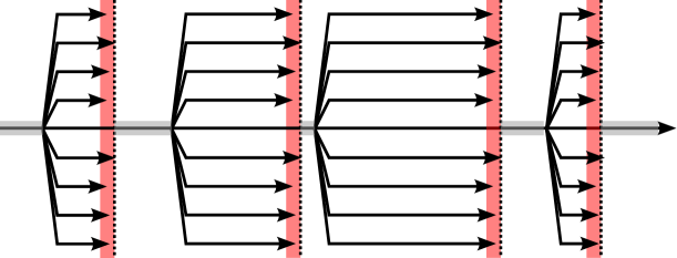
Fig. 1: Branch-and-bound parallelism as is commonly used in OpenMP. The horizontal arrows indicate the program flow over time, and branching arrows indicate a parallel section. The dotted vertical bars are the synchronization points at the end of each such section. Parallel efficiency is lost to two factors: The grey shaded areas along the main horizontal area indicate parts of the program that do not execute in parallel and restrict the maximum parallel efficiency, e.g. as described by Amdahl’s law, and the red areas indicate the difference between the fastest and slowest threads in each parallel block, i.e. the time lost to individual thread load imbalances and synchronization.

In order to better exploit shared-memory parallelism, a different paradigm is needed, i.e. instead of annotating an essentially serial computation with parallel bits, it is preferable to describe the entire computation in a way that is inherently parallelizable. One such approach is task-based parallelism, in which the computation is divided into a number of computational tasks, which are then dynamically allocated to a number of processors. In order to ensure that the tasks are executed in the right order, e.g. that data needed by one task is only used once it has been produced by another task, and that no two tasks update the same data at the same time, dependencies between tasks are specified and strictly enforced by a task scheduler.

Such a set of tasks and dependencies form a Directed Acyclic Graph (DAG), which the processors can traverse in topological order, picking up and executing tasks when they have no unresolved dependencies. Whenever a processor is done with a task, it goes back to the DAG and looks for a new one or waits until a task becomes available, until all tasks have been completed.

Figure 2 shows five tasks, A, B, C, D, and E, drawn as circles, and their dependencies, depicted as arrows. In this example, tasks B and C depend on task A, and task D depends on task B. In a task-based parallel environment, tasks A and E could be executed first, as they have no unresolved dependencies. Once task A has been executed, tasks B and C become available. Task D can only be executed once task B has completed.

Fig. 2: Five tasks, A, B, C, D, and E, with their dependencies shown as arrows, i.e. tasks B and C both depend on task A.

Several middle-wares providing such task-based parallelism exist, e.g. Cilk [8], QUARK [37], StarPU [4], SMP Superscalar [1], OpenMP 3.0 [14], and Intel’s TBB [28]. Cilk and StarPU are implemented as extensions to the C programming language, whereas SMP Superscalar and OpenMP 3.0 use so-called pragmas to define functions or sections of code that form tasks. QUARK and Intel’s TBB are implemented as compiler-independent libraries which provide functionality for creating and executing tasks.

The main advantages of using a task-based approach are

• The order in which the tasks are processed is completely dynamic and adapts automatically to load imbalances.

• If the dependencies and conflicts are specified correctly, there is no need for expensive explicit locking, synchronization, or atomic operations to deal with most concurrency problems.

• Each task has exclusive access to the data it is working on, thus improving cache locality and efficiency. If each task operates exclusively on a restricted part of the problem data, this can lead to hich cache locality and efficiency.

Despite these advantages, task-based parallelism is only rarely used in scientific codes, with the notable exception of the PLASMA project [2], which is the driving force behind the QUARK library, and the deal.II project [6] which uses Intel’s TBB. This is most probably due to the fact that, in order to profit from the many advantages of task-based programming, for most non-trivial problems, the underlying algorithms must be redesigned from the bottom up in a task-based way.

3 Algorithms

In the following, I will describe both an extension to the traditional task-based parallel programming model, as well as a task-based formulation for neighbour-finding and particle interactions in SPH simulation.

3.1 Task-based parallelism with conflicts

I will differ from previous approaches to task-based parallelism in introducing the concept of conflicts between tasks. Conflicts occur when two tasks operate on the same data, but the order in which these operations must occur is not defined. Figure 3 extends the example in the previous section with conflicts between tasks B and C, and tasks D and E. In a parallel setup, once task A has been completed, if one processor picks up task B, then no other processor is allowed to execute task C until task B has completed, or vice versa.

Fig. 3: Five tasks, A, B, C, D, and E, with their dependencies shown as arrows, and their conflicts shown as dashed lines, i.e. tasks B and C, and tasks D and E conflict with each other.

In previous task-based models, conflicts can be modeled by adding dependencies between conflicting tasks, yet this introduces an artificial ordering between the tasks and imposes unnecessary constraints on the task scheduler (e.g. mutual and non-mutual interactions in [24]).

In the following, conflicts are modelled using exclusive locks on shared resources, i.e. a task operating on potentially shared data will only be scheduled if the executing thread can obtain an exclusive lock on that data, thus preventing other tasks using said data to be scheduled concurrently. This locking mechanism will be described in more detail further on.

3.2 Spatial decomposition

Besides the problems described in the previous section, spatial trees also have the disadvantage that they do not lend themselves particularly well for task-based computations. Therefore, in the following, the particle interactions will be described in terms of hierarchical cell lists, and the operations thereon.

If $h_{\mathsf{max}}:=\max_{i}h_{i}$ is the maximum smoothing length of any particle in the simulation, the simulation domain is split into rectangular cells of edge length larger or equal to $h_{\mathsf{max}}$.

Given such an initial decomposition, a list of cell self-interactions, which contains all non-empty cells in the grid, is generated. This list of interactions is then extended by the cell pair-interactions, i.e. a list of all non-empty cell pairs sharing either a face, edge, or corner. For periodic domains, cell pair-interactions must also be specified for cell neighbouring each other across periodic boundaries.

In this first coarse decomposition, if a particle $p_{j}$ is within range of a particle $p_{i}$, both will be either in the same cell, or in neighbouring cells for which a cell self-interaction or cell pair-interaction has been specified respectively. These self- and pair-interactions therefore encode, conceptually at least, the evaluation of the interactions between all particles in the same cell, or all interactions between particle pairs spanning a pair of cells, respectively, i.e. if the list of self-interactions and pair-interactions are traversed, computing all the interactions within each cell and between each cell pair, respectively, the all the required particle interactions will have been computed.

In the best case, i.e. if each cell contains only particles with smoothing length equal to the cell edge length, if for any particle $p_{i}$ each particle $p_{j}$ in the same and neighbouring cells is inspected, only roughly 16% of the $p_{j}$ will actually be within range of $p_{i}$ [17]. If the cells contain particles who’s smoothing length is less than the cell edge length, this ratio only gets worse. It therefore makes sense to refine the cell decomposition recursively, bisecting each cell along all spatial dimension whenever (a) the cell contains more than some minimal number of particles, and (b) the smoothing length of a reasonable fraction of the particles within the cell is less than half the cell edge length. A cell will be referred to as split if it has been divided into sub-cells.

After the cells have been split, the cell self-interactions of each cell can be split up into the self-interaction of its sub-cells and the pair-interactions between them (see Figure 5). Likewise, the cell pair-interactions between two cells that have been split can themselves be split up into the pair-interactions of the sub-cells spanning the original pair boundary (see Figure 6) if, and only if, all particles in both cells have a smoothing length of less than half the cell edge length. If only one cell within a cell pair-interaction has been split, then the cell pair-interaction is preserved, i.e. the interactions between the particles in both cells are computed, yet the split cell is considered as a whole.

If the cells, self-interactions, and pair-interactions are split in such a way, if two particles are within range of each other, they will (a) either share a cell for which a cell self-interaction is defined, or (b) they will be located in two cells which share a cell pair-interaction. In order to identify all the particles within range of each other, it is therefore sufficient to traverse the list of self-interactions and pair-interactions, and to compute the interactions therein.

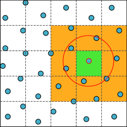
Fig. 4: Initial spatial decomposition: The space is divided into cells of edge length greater or equal to the largest smoothing length in the system. All neighbours of any given particle (small red circle) within that particle’s smoothing length (large red circle) are guaranteed to lie either within that particle’s own cell (green) or the directly adjacent cells (orange).

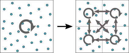
Fig. 5: Large cells can be split, and their self-interaction replaced by the self- and pair-interactions of their sub-cells.

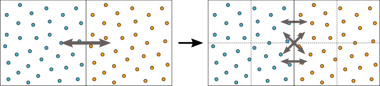
Fig. 6: If all particles in a pair of interacting cells have a smoothing length less or equal to half of the cell edge length, both cells can be split, and their pair-interaction replaced by the pair-interactions of the neighbouring sub-cells across the interface.

3.3 Particle interactions

The interactions between all particles within the same cell, i.e. the cell’s self-interaction, can be computed by means of a double for-loop over the cell’s particle array. The algorithm, in C-like pseudo code, can be written as follows:

⬇

1for (i = 0; i < count - 1; i++) {

2 for (j = i + 1; j < count; j++) {

3 rij = || parts[i] - parts[j] ||.

4 if (rij < h[i] || rij < h[j]) {

5 compute interaction.

6 }

7 }

8}

where count is the number of particles in the cell and parts and h refers to an array of those particles’ positions and their smoothing lengths respectively.

The interactions between all particles in a pair of cells can be computed similarly, e.g.:

⬇

1for (i = 0; i < count_i; i++) {

2 for (j = 0; j < count_j; j++) {

3 rij = || parts_i[i] - parts_j[j] ||.

4 if (rij < h_i[i] || rij < h_j[j]) {

5 compute interaction.

6 }

7 }

8}

where count_i and count_j refer to the number of particles in each cell and parts_i and parts_j, and h_i and h_j, refer to the particles of each cell and their smoothing lengths respectively.

As described in [17], though, using this naive double for-loop, only roughly $33.5\%$, $16.2\%$, and $3.6\%$ of all particle pairs between cells sharing a common face, edge, or corner, respectively, will be within range of each other, leading to an excessive number of spurious pairwise distance evaluations (line 3). The sorted cell interactions described therein will be used in order to avoid this problem, yet with some minor modifications, as the original algorithm is designed for systems in which the smoothing lengths of all particles are equal: The particles in both cells are first sorted along the vector joining the centers of the two cells, then the parts $p_{i}$ on the left are interacted with the sorted parts $p_{j}$ on the right which are within $h_{i}$ along the cell pair axis. The same procedure is repeated for each particle $p_{j}$ on the right, interacting with each other particle $p_{i}$ on the left, which is within $h_{j}$, but not within $h_{i}$, along the cell pair axis (see Figure 7). The resulting algorithm, in C-like pseudo-code, can be written as follows:

⬇

1r_i = parts_i projected onto the cell pair axis

2r_j = parts_j projected onto the cell pair axis

3ind_i = indices of parts_i sorted w.r.t. r_i in ascending order

4ind_j = indices of parts_j sorted w.r.t. r_j in ascending order

5for (i = 0; i < count_i; i++) {

6 for (jj = 0; jj < count_j; jj++) {

7 j = ind_j[jj];

8 if (r_i[i] + h_i[i] < r_j[j]) break;

9 rij = || parts_i[i] - parts_j[j] ||.

10 if (rij < h_i[i]) {

11 compute interaction.

12 }

13 }

14}

15for (j = 0; j < count_j; j++) {

16 for (ii = count_i - 1; ii >= 0; ii--) {

17 i = ind_i[i];

18 if (r_i[i] < r_j[j] - h_j[j]) break;

19 rij = || parts_i[i] - parts_j[j] ||.

20 if (rij < h_j[j] && rij > h_i[i]) {

21 compute interaction.

22 }

23 }

24}

where r_i and r_j contains the position the particles of both cells along the cell axis, and ind_i and ind_j contain the particle indices sorted with respect to these positions respectively. The if-statements in lines 9 and 19 are needed to check if there are any particles left within range along the cell pair axis, and to prematurely exit the innermost loop if this is not the case.

The particles need to be traversed twice: once to identify all particles in range of the particles on the left (lines 5–14), and once to identify all particles in range of the particles on the right (lines 15–24), but that were not identified in the first loop, thus the condition in line 20. Instead of sorting the particles every time the pairwise interactions between two cells are computed, the sorted indices along the 26 possible cell-pair axes can be pre-computed and stored for each cell. These sorted indices are, however, symmetric: e.g. the indices computed for a cell interacting with a cell to its left along the $x$-axis are the inverse of the indices required for interacting with the cell on its right. It is therefore only necessary to sort 13 sets of indices, and flip the cells in a cell pair-interaction around when the order required is the opposite of the order stored, i.e. as is done in [19].

This may still seem like quite a bit of sorting, especially for the larger, higher-level cells in the simulation. If, however, a cell is split and its sub-cells have been sorted, the sorted indices of the higher-level cells can be constructed by shifting and merging the indices of its eight sub-cells (see Figure 8). For cells with sub-cells, this reduces the ${\mathcal{O}}(n\log{n})$ cost of sorting to ${\mathcal{O}}(n)$ for merging.

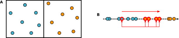
Fig. 7: Sorted cell pair-interactions. (A) Starting from a pair of neighbouring cells, (B) the particles from both cells are projected onto the axis joining the centers of the two cells. The particles on the left (blue) and right (orange) are then sorted in descending and ascending order respectively. Each particle on the left is then only interacted with the particles on the right within the cutoff radius along the cell axis.

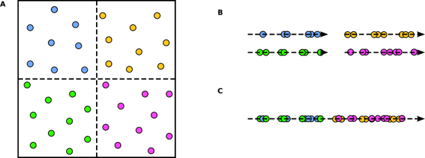
Fig. 8: Hierarchical cell sorting of (A) a split cell. (B) The sub-cells are first sorted individually and (C) shifted and merged to produce the sorted list of the parent cell.

3.4 Task-based implementation

The particle interactions described in the previous subsection lead to three basic task types:

• Cell sorting, in which the particles in a given cell are sorted with respect to their position along the 13 cardinal axes, as described in [19].

• Cell self-interaction, in which all the particles of a given cell are interacted with all the other particles within the same cell,

• Cell pair-interaction, in which the interactions for all particle pairs spanning a pair of cells are computed.

In order to reduce the total number of tasks, as well as to increase their locality, pair- and self-interactions involving less than a certain number of particles are split only implicitly, i.e. the tasks resulting from a split are grouped together and executed as a single task.

The self-interaction and pair-interaction tasks exist in two flavors, one for the density computation (see (2)) and one for the force computation (see (4)). Each pair-interaction task requires the sorted indices of the particles in each cell provided by the sorting tasks. Since the tasks are restricted to operating on the data of a single cell, or pair of cells, two tasks conflict if they operate on overlapping sets of cells. Due to the hierarchical nature of the spatial decomposition, two tasks also conflict if any of the cells used by one task are sub-cells of any of the cells used by the other task.

The interactions have two phases, the density and force computation, which need to be clearly separated, i.e. all the density tasks on a cell must complete before its force tasks, which rely on the densities, can be computed. They are therefore separated by a ghost task for each cell. This ghost task depends on all the density computations for a given cell, and, in turn, all force computations involving that cell depend on its ghost task. This mechanism enforces that all density computations for a set of particles have completed before this density is used in any force computations.

Finally, an integrator task for each cell is used to update the particle positions, velocities, and internal energy once the force equations of the particles therein have been evaluated.

The dependencies and conflicts between the different task types, which are illustrated in Figure 9, can be formulated as follows:

• Each cell sorting task on a cell with sub-cells depends on the sorting tasks of all its sub-cells.

• Each cell pair-interaction task depends on the cell sorting tasks of both its cells.

• Cell pair-interaction and cell self-interaction tasks operating on overlapping sets of cells or sub-cells conflict with each other.

• The ghost task of each cell depends on all the density cell pair interactions and self-interactions which involve the particles in that cell.

• The ghost task of each cell depends on the ghost tasks of its sub-cells.

• Each force cell pair-interaction or self-interaction task depends on the ghost tasks of the cells on which it operates.

• Each integrator task depends on the force cell pair-interaction and self-interaction tasks of its cell and of all its cell’s sub-cells.

This task decomposition has significant advantages over the use of spatial trees. First of all, the cost of identifying all particles in range of a given particle does not depend on the total number of particles, but only on the local particle density. Furthermore, the particle interactions in each task are computed symmetrically, i.e. each particle pair is identified only once for each interaction type. The sorted particle indices can be re-used for both the density and force computation, and even over several time-steps [19], thus reducing the computational cost even further. Finally, if the particles are stored grouped by cell, each task then only involves accessing and modifying a limited and contiguous region of memory, thus greatly improving cache re-use [15].

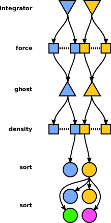
Fig. 9: Task dependencies and conflicts: Arrows indicate the dependencies between different task types, i.e. and arrow from task A to task B indicates that A depends on B. Dashed lines between tasks indicate conflicts, i.e. the two tasks can not be executed concurrently. Each sort task (circles) depends only on the sort tasks of its sub-cells. The pair-interactions (rectangles) for the particle density computation depend on the sort tasks of the respective cells, whereas self-interaction tasks (squares) for the density computation do not, as they do not require sorting. Self- and pair-Interactions on overlapping cells (same color) conflict with each other. The ghost task of each cell (triangles) depends on the self- and pair-interaction density tasks. The self- and pair-interaction tasks for the force computation, depend on the ghost tasks of the respective cells, and the integrator task (inverted triangle) of each cell depends on the cell’s force tasks.

3.4.1 Task scheduling

The assignment of individual tasks to the processors of a system is a tricky issue: Each task must be scheduled once all its dependencies are met, only if it has no conflicts, and only to a single processor. Additionally, the tasks should be scheduled in a way that maximizes both the amount of non-conflicting tasks available to all processors, as well as the amount of cache re-use between tasks.

In the current implementation, tasks are represented as follows:

⬇

1struct task {

2 int type;

3 int wait;

4 int nr_unlocks;

5 struct task *unlocks;

6 ...

7};

where type is determines the task type, e.g. sorting, pair, or ghost tasks. The variable wait is a counter for the number of unresolved dependencies belonging to this task and will be zero when this task is ready to run. Conversely, unlocks is an array of nr_unlocks pointers to tasks that depend on this task. The tasks also contain additional data specific to each task type, i.e. the cells on which it operates.

The wait counters, which are initialized to zero, are set before the computation by traversing the list of tasks, and, for each task, incrementing by one the wait counter of each of its unlocks tasks. The wait counter then holds the number of other tasks on which the task depends. Once a task has been executed, the wait counters of its unlocks tasks are decremented by one. If a task’s wait counter is zero, then it has no unsatisfied dependencies and can be executed.

As opposed to the dependencies, the task conflicts are not encoded explicitly, but implemented via locks on shared resources, i.e. the cells on which a task operates. This locking is described in detail in Section 3.4.2.

The tasks are managed by a scheduler, which assigns tasks whose dependencies have all been met to different queues. The processors, or threads, in a system then obtain the tasks directly from this scheduler, which tries to obtain a task from the thread’s preferred queue. If this queue is empty or has no conflict-free tasks, the scheduler attempts to obtain a task from any other non-empty queue. This is, in essence, the well-known concept of work-stealing described in [9].

In order to preserve memory locality and improve cache re-use, the scheduler attempts to assign tasks working on similar sets of cells to the same queue. This is done by assigning each cell a pre-defined preferred queue. Tasks involving only cells of a given queue are assigned to that queue, and tasks involving more than one queue are assigned to the shortest of the set of queues.

While the scheduler is responsible for dependencies and data locality, the queues themselves are responsible for conflict avoidance and task order. The queues are implemented as binary heaps which order the tasks according to their weight. A task’s weight is defined as the approximate or measured computational cost of the task, plus the maximum weight of all its dependent tasks. This weight is a measure for the length of the critical execution path starting at the given task. Picking the task with the largest weight corresponds to reducing the longest critical path of the task DAG first.

When a processor requests a task from a queue, the heap is traversed in topological order, starting from the top, looking for tasks free of conflicts. Although the first task inspected will have the largest weight in the queue, the traversal is not in strictly decreasing weight order. This sub-optimal traversal was chosen as a efficiency trade-off, since the cost of inserting or removing an element in a binary heap is in ${\mathcal{O}}(\log n)$, whereas maintaining a strict ordering requires at least ${\mathcal{O}}(n)$ for insertion, e.g. using linked lists. In order to ensure that each task is assigned only once, mutexes are used to control exclusive access to each queue.

The details of the task scheduler are further described in a separate publication [20].

3.4.2 Cell locking

Particles within a cell are also within that cell’s hierarchical parents. Therefore, when working on the particles of a cell, tasks which operate on its parent’s data should not be allowed to execute. One way to avoid this problem is to require that a task not only lock a cell, but also all of its hierarchical parents in order to operate on its data. This, however, would prevent tasks involving siblings who share a common hierarchical parent cell, yet whose particle sets do not overlap, from executing.

This problem is avoided by giving each cell both a lock, and a hold counter: A cell is locked when it, or one of its parent cells, is currently in use. A cell is held when one or more of its sub-cells is locked, and thus cannot be locked itself. Since more than one task at a time may hold a cell, this property is implemented as a counter.

The cell locking/holding is implemented as follows:

⬇

1int cell_locktree(struct cell c) {

2 struct cell *c1, *c2;

3 if (trylock(c->lock) != 0) return 1;

4 if (c->hold > 0) {

5 unlock(c->lock)

6 return 1;

7 }

8 for (c1 = c->parent; c1 != NULL; c1 = c1->parent) {

9 if (trylock(c1->lock) != 0) break;

10 atomic_add(c1->hold, 1);

11 unlock(c1->lock);

12 }

13 if (finger != NULL) {

14 for (c2 = c->parent; c2 != c1; c2 = c2->parent) {

15 atomic_sub(c2->hold, 1);

16 }

17 unlock(c->lock);

18 return 1;

19 } else {

20 return 0;

21 }

22}

When trying to lock a cell, the function first checks that it is neither locked (line 3) or held (line 4), i.e. its hold counter is zero. If neither is the case, then the cell can be locked. It then travels up the hierarchy increasing the hold counter of each cell on the way, up to the topmost cell (lines 8–12). If any cell along the hierarchy is locked (line 9), the locking is aborted and all locks and holds are undone (lines 13–18, see Figure 10). The operations atomic_add and atomic_sub are understood, respectively, to increase or decrease a value atomically.

When the cell is released, its lock is unlocked and the hold counter of all hierarchical parents is decreased by one:

⬇

1void cell_unlocktree ( struct cell c ) {

2 struct cell *c1;

3 unlock( c->lock )

4 for ( c1 = c->parent ; c1 != NULL ; c1 = c1->parent )

5 atomic_sub( c1->hold , 1 );

6 }

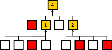
Fig. 10: Example of hierarchical cell locking. The cells marked in red are “locked” while the cells marked in yellow have a “hold” count larger than zero. The hold count is shown inside each cell and corresponds to the number of locked cells hierarchically below it. All cells except for those locked, below a locked cell, or with a “hold” count larger than zero can still be locked without violating any constraints.

3.5 Hybrid shared/distributed-memory parallelism

Although the task-based algorithms described in the previous subsections were described only in the context of shared-memory parallelism, the task-based scheme extends rather elegantly to hybrid shared/distributed-memory parallel setups as well.

The highest-level cells in the hierarchical cell lists can be distributed between a set of distributed-memory nodes, such that for each node the space is partitioned into local and foreign cells. On each node, the tasks are constructed as in the single-node case, yet each node only keeps the tasks which involve at least one local cell, i.e. self interaction, ghost, and integrator tasks on local cells, and pair interaction tasks involving two local cells, or a local and a foreign cell. This step would seem to imply that each node would have to have information on all particles in the system, but it is actually sufficient for it to know only the structure of the cell hierarchy of the highest-level foreign cells adjacent to a local cell.

The set of foreign cells which are involved in a pair interaction with a local cell will be referred to as proxy cells. These cells are used to compute interactions locally, but contain particles which reside on a different node.

For each proxy cell, two communication tasks are generated, one to receive the particle positions and other data for the density computation, and one to receive the particle densities and other data for the force computation. The force and density tasks involving each proxy cell are made dependent of these two communication tasks respectively. If a proxy cell requires a sort task, the sort task is also made dependent of the communication task for the particle positions (see Figure 11).

Similarly, for each local cell which is a proxy cell on another node, two communication tasks are generated to send the particle positions and densities respectively to the foreign node. The communication task sending a cell’s particle positions has no dependencies, but care must be taken to make any task that will update the particle data, i.e. the cell’s ghost task, depend on its completion to avoid corrupting the particle data before it is sent. The communication task sending a cell’s particle densities depends on the computation of said densities, i.e. the cell’s ghost task. Since the cell’s integrator task will modify the particle data, it must be made dependent on the completion of the communication task sending the cell’s particle densities.

All communication is implemented asynchronously using the MPI_Isend, MPI_Irecv, and MPI_Test commands. The MPI_Isend and MPI_Irecv commands for a communication task are emitted as soon as the task’s dependencies have been met and it is enqueued. Once in the task queue, the communication tasks are only executed if a call to MPI_Test returns that they have indeed completed. The tasks themselves do nothing else, i.e. all the work happens in the background or on the calls to MPI_Test, depending on how asynchronous communication is implemented in the underlying MPI library.

Contrary to most distributed-memory parallel codes, the communication between two nodes is not grouped into a single MPI send/recv command. Using individual communication tasks has the advantage that the particle data, which is stored contiguously for each cell, does not need to be re-packaged for communication. It also has the advantage of preventing bottlenecks, since a single monolithic sending task would have to wait for all density tasks involving a different node to complete before it could be executed. The only potential disadvantage is that the sum of the latencies for several small sends and receives is far larger than the latency for a single large send and receive. This, however, should be of no particular concern as the task-based model can just execute other tasks while waiting for the data to be transmitted, effectively masking any communication latencies.

The main advantage of using non-blocking communication primitives and a task based model over the traditional synchronous communication in other distributed-memory parallel codes is twofold: Firstly, since the computation is data driven, there are no fixed synchronization points between nodes, which could force all the nodes to wait until the slowest node is ready. Secondly, the communication latencies are completely hidden i.e. instead of waiting idly for data to be transmitted, the cores of a node can execute any other task, if available, in the meantime.

One final advantage associated with using the task-based formulation for hybrid simulations has to do with the domain decomposition, which was until here simply assumed to be given. In most parallel codes, the domain is decomposed following the simulation data, i.e. attempting to spread the particles evenly amongst the nodes. The tasks, however, form a complete representation of the work that will actually be done during the computation, which can be modelled as a graph in which each cell is a node, and two nodes share an edge if they are spanned by a pair-interaction task. The node weights in the graph are given by the sum of the approximate costs of all tasks involving only that node, and the edge weights by the sum of the approximate costs of the tasks spanning both nodes’ cells. This graph can then be partitioned using a standard library such as METIS [22] providing a good equidistribution of the actual work across the nodes, as opposed to just the data.

Figure 12 shows the task timeline for a single time-step of a hybrid shared/distributed-memory parallel simulation of 1 M particles on a perturbed grid on eight 12-core nodes of the COSMA4 cluster. The different colors indicate the different task types. The white gaps preceding the red communication tasks are time spent in the MPI_Test function. Note that despite the large degree of parallelization (96 cores, $<90$ ms per time step), the load distribution between nodes is good an the load balance within each node is almost perfect, despite the uneven communication costs.

It should be noted that the hybrid approach will still suffer from the same surface-to-volume ratio problem for distributed computations described in the introduction. However, as opposed to purely distributed-memory parallel based codes, the problem is somewhat mitigated by the fact that the hybrid approach uses one MPI node per physical node, as opposed to one MPI node per core, and that the commuication latencies can be overlapped with computations over local cells. With the increasing number of cores per cluster node, this significantly reduces the ratio of communication per computation.

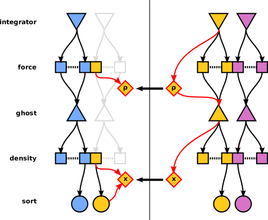
Fig. 11: Task dependencies and conflicts for hybrid parallelism: Two task hierarchies on neighbouring nodes. The blue cell, which resides on the left node, interacts with the yellow cell, which resides on the right node. The regular task hierarchy of the “ghost” yellow cell on the left is replaced with communication tasks (yellow diamonds) and new dependencies (red arrows) on both nodes. On the left node, the sorting and density tasks for the yellow cell depend on the receipt of the particle positions (marked “x”). Similarly, the force tasks depend on the receipt of the particle densities (marked “$\boldsymbol{\rho}$”). On the right node, the sending of the particle densities depends on the cell’s ghost task to ensure that they have been effectively computed. The ghost and integrator tasks on the right, which overwrite parts of the particle data, are made to depend on the communication tasks having completed.

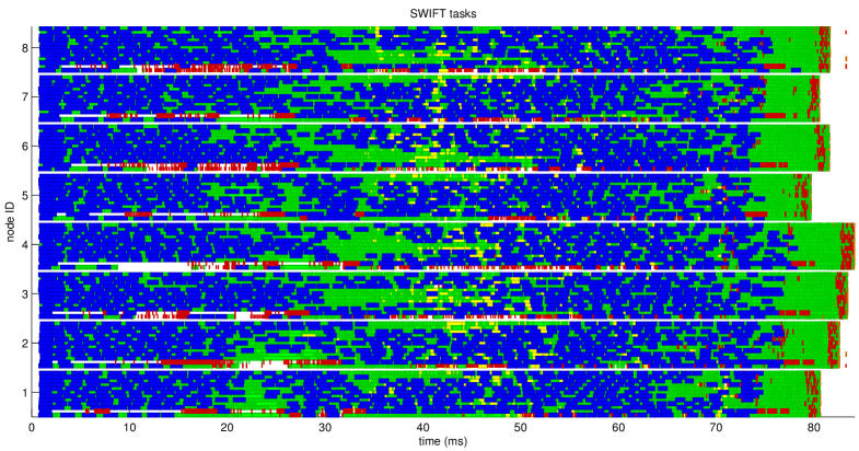
Fig. 12: Task timeline for a single time-step of a hybrid shared/distributed-memory parallel simulation on eight 12-core nodes of the COSMA4 cluster. Each task is represented by a block, the color of which represents the task type, i.e. pair-interaction (blue), self-interaction (green), ghost (yellow), communication (red), and integration (orange).

4 Validation

This section describes how the algorithms shown in the previous section are implemented and tested against exiting codes on specific problems.

4.1 Implementation details

The algorithms described above are all implemented as part of SWIFT (SPH With Inter-dependent Fine-grained Tasking), an Open-Source platform for hybrid shared/distributed-memory SPH simulations. The code is being developed in collaboration with the Institute of Computational Cosmology (ICC) at Durham University.

SWIFT is implemented in C, and can be compiled with the gcc compiler. Although explicitly SIMD-vectorized code, using the gcc vector types and SSE/AVX intrinsics, has been implemented, it was switched off in the following to allow for a fair comparison with Gadget-2, which does not use explicit vectorization.

The underlying multithreading for the task-based parallelism is implemented using standard pthreads [11]. Each thread is assigned it’s own task queue. The threads executing the tasks are initialized once at the start of the simulation and synchronize via a barrier between time steps. The task selection is implemented as described above, yet with the addition that the ID of the last thread to have worked on each cell is recorded and the queue inspects up to 50 valid tasks looking for one that involves previously-used cells.

The equations of motion are integrated using a velocity-Verlet integrator. Multiple time-stepping has been implemented similarly to the Gadget-2 code [32]: The maximum time-step for each particle is computed as

$$\Delta t_{i}=C_{CFL}\frac{2h_{i}}{\max_{j}\left(c_{i}+c_{j}+\max\{0,-3\mathbf{r}_{ij}\cdot\mathbf{v}_{ij}/r_{ij}\}\right)}$$ (6)

where $\mathbf{v}_{ij}=\mathbf{v}_{i}-\mathbf{v}_{j}$, $\mathbf{r}_{ij}=\mathbf{r}_{i}-\mathbf{r}_{j}$, and $c_{i}$ and $c_{j}$ are the speed of sound of the respective interacting particles. The CFL constant $C_{CFL}$ is usually set to $\sim 0.3$. Given a base time-step $\Delta t$, particles for which $2^{k-1}\Delta t<\Delta t_{i}\leq 2^{k}\Delta t$ are only active, i.e. included in the density and force calculations, every $2^{k}$th step. Tasks which do not involve any cell with active particles, and are not dependencies of any tasks with active particles, are omitted from the task list in each step.

SWIFT also implements the pseudo-Verlet lists described in [19]: The spatial decomposition is computed once and then used over several time-steps until they are invalidated by particle movement. The sorted particle indices for each cell are computed and stored whenever the cells are updated, and re-used over subsequent time-steps. If the cell decomposition does not need to be re-computed often, this can lead to substantial savings by eliminating the sort tasks in these time-steps.

Finally, SWIFT also implements an artificial viscosity of the Monaghan–Balsara type [26, 5], i.e. the terms

$$\frac{dv_{i}}{dt} = -\frac{1}{4}\sum_{r_{ij}<\hat{h}_{ij}}m_{j}\Pi_{ij}\left({\nabla_{r}}W({r}_{ij},h_{i})+{\nabla_{r}}W({r}_{ij},h_{j})\right)(f_{i}+f_{j}),$$

$$\frac{du_{i}}{dt} = \frac{1}{8}\sum_{r_{ij}<\hat{h}_{ij}}m_{j}\Pi_{ij}(\mathbf{v}_{i}-\mathbf{v}_{j})\left({\nabla_{r}}W({r}_{ij},h_{i})+{\nabla_{r}}W({r}_{ij},h_{j})\right)(f_{i}+f_{j}),$$

are added to (4) and (5) respectively, where

$$\Pi_{ij} = -\alpha\frac{\left(c_{i}+c_{j}-3w_{ij}\right)w_{ij}}{\rho_{i}+\rho_{j}},$$

$$w_{ij} = \min\left\{0,\mathbf{v}_{ij}\cdot\mathbf{r}_{ij}/r_{ij}\right\},$$

$$f_{i} = \frac{|\nabla\times\mathbf{v}_{i}|}{|\nabla\cdot\mathbf{v}_{i}|+|\nabla\times\mathbf{v}_{i}|+10^{-4}\frac{c_{j}}{h_{j}}},$$

$$\nabla\times\mathbf{v}_{i} = -\frac{1}{\rho_{i}}\sum_{j}m_{j}(\mathbf{v}_{j}-\mathbf{v}_{i})\times{\nabla_{r}}W({r}_{ij},h_{i}),$$

$$\nabla\cdot\mathbf{v}_{i} = \frac{1}{\rho_{i}}\sum_{j}m_{j}(\mathbf{v}_{j}-\mathbf{v}_{i})\cdot{\nabla_{r}}W({r}_{ij},h_{i}).$$

and the viscosity parameter $\alpha$ is usually chosen in the range $[0.5,2]$.

4.2 Simulation setup

In order to test their accuracy, efficiency, and scaling, the algorithms described in the previous section were tested in SWIFT using the following four simulation setups:

• Sod-shock [31]: A rectangular periodic domain of size $8\times 1\times 1$ containing a high-density region of 800 000 particles with $P_{i}=1$ and $\rho_{i}=4$ on one half, and a low-density region of 200 000 particles with $P_{i}=0.1795$ and $\rho_{i}=1$ on the other. The simulation results can be compared to an analytic solution, providing a test case for the accuracy of the implementation.

• Sedov blast: A face-centered cubic lattice of $101\times 101\times 101$ particles at rest with $P_{i}$ and $\rho_{i}=1$, yet with the central 26 particles set to $P_{i}=100$. The resulting blast wave provides a good example of strong pressure, density, and smoothing length gradients for which an analytical solution can be computed.

• Cosmological box: Realistic distribution of matter in a periodic volume of universe at redshift $z=0.5$. The simulation consists of $\sim$51 M particles with a mix of smoothing lengths spanning three orders of magnitude, providing a test-case for neighbour finding and parallel scaling in a real-world scenario. Although cosmological simulations are often run with billions of particles [32], the number of particles used is sufficient for the study of a number of interesting phenomenon.

In all simulations, the constants $N_{ngb}=48$, $\gamma=5/3$, $C_{CFL}=1/4$, and $\alpha=0.8$ were used. In SWIFT, cells were split if they contained more than 300 particles and more than 87.5% of the particles had a smoothing length less than half the cell edge length. Fr cells or cell pairs containing less than 6000 particles, the tasks hierarchically below them were grouped into a single task.

The Sod-shock simulation was run both with and without the sorted particle interaction in order to provide a rough comparison to traditional neighbour-finding approaches in SPH simulations with locally constant smoothing lengths. In all three test cases, results were computed using a fixed time step and updating the forces on all particles in each time-step. In the Sedov blast simulation, the timestep was set to be below the smallest particle timestep as computed in (6) in each step.

The simulation results compared with Gadget-2 [32] in terms of speed and parallel scaling. Gadget-2 was compiled with the Intel C Compiler version 2013.0.028 using the options

-DUSE_IRECV -O3 -ip -fp-model fast -ftz -no-prec-div -mcmodel=medium.

SWIFT v. 1.0.0 was compiled with the GNU C Compiler version 4.8 using the options

-O3 -ffast-math -fstrict-aliasing -ftree-vectorize -funroll-loops -mmmx -msse -msse2 -msse3 -mssse3 -msse4.1 -msse4.2 -mavx -fopenmp -march=native -pthread.

Note that although the compiler switches for the SSE and AVX vector instruction sets were activated, explicit SIMD-vectorization, using vector types and/or intrinsics, was not enabled. For the hybrid shared/distributed memory parallel runs, Platform MPI version 9.1.0 was used.

All simulations were run on the COSMA5 supercomputer, consisting of 420 quad-Intel Xeon E5-2670 16-core nodes running at 2.6 GHz with CentOS release 6.2 Linux for x86_64. The nodes are connected via Mellanox FDR10 Infiniband in a 2:1 blocking configuration.

4.3 Results

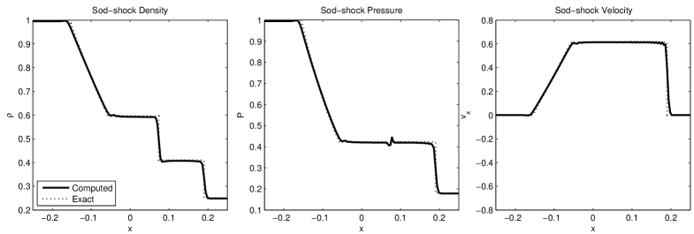
Fig. 13: Results for the Sod-shock simulation test case at $t=0.12$. The density, pressure, and velocity profiles are in good agreement with the analytic solution (top). The simulation scales well up to 16 cores of the same shared-memory machine, achieving 86% parallel efficiency (bottom).

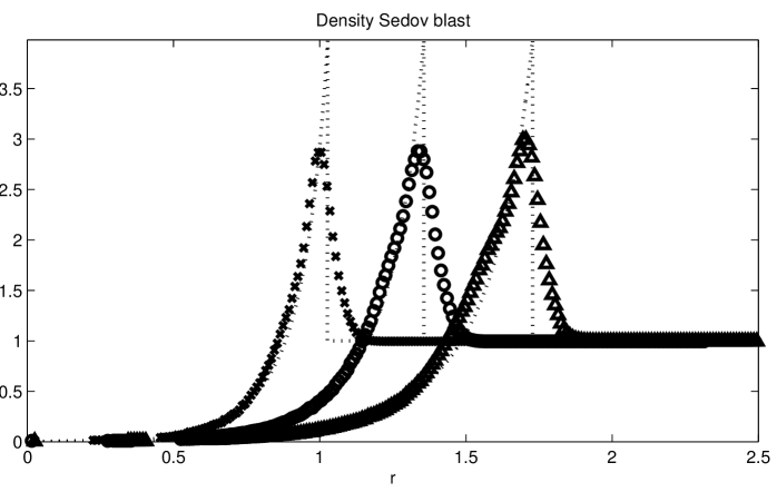
Fig. 14: Radial density profile of the Sedov blast simulations at times $t=0.075$ (crosses), $t=0.150$ (circles), and $t=0.275$ (triangles), along with the corresponding analytically computed solution (dotted lines).

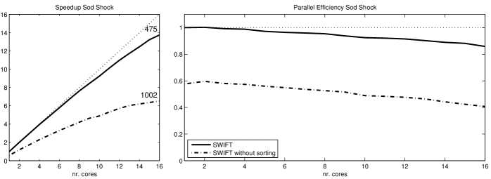
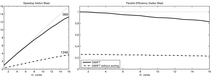
Fig. 15: Parallel (strong) scaling and efficiency plots for the Sod-shock and Sedov blast simulations on up to 16 cores of a $4\times$Intel Xeon E5-2670 at 2.6 GHz. The numbers inside the speedup plots on the left are the average number of milliseconds per timestep.

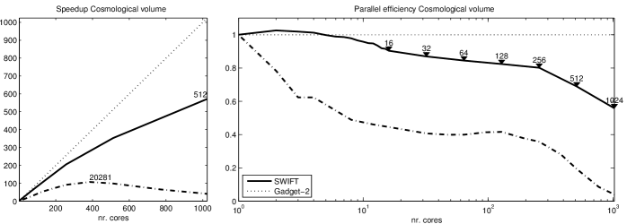
Fig. 16: Hybrid parallel (strong) scaling and efficiency for the Cosmological volume simulation on up to 64 nodes of the COSMA5 cluster, containing 16 cores each, for both SWIFT and Gadget-2. The numbers in the scaling plot on the left represent the minimum average milliseconds per timestep achieved. The inverted triangles and numbers in the efficiency plot point to the number of cores used at each point. For both codes, the parallel efficiency is computed relative to the performance of each code on a single core.

Figure 13 shows the averaged density, pressure, and velocity profiles along the $x$-axis of the Sod-shock simulation at time $t=0.12$. The computed results are compareable to those produced with Gadget-2 for the same setup and in good agreement with the analytical solution [31].

Similarly, Figure 14 shows the average radial density profiles for the Sedov blast simulation at times $t=0.075$, $t=0.150$, and $t=0.275$, along with their analytical solutions [29].

Figure 15 shows the performance of the shared-memory task-based code on a single 16-core node of the COSMA5 cluster. In both cases, SWIFT achieves over 80% parallel efficiency on all 16 cores. The Sod-shock and Sedov blast simulations without the sorted interactions described in Section 3.3 are roughly $\sim 2-4\times$ slower than the simulation with sorted interactions. It should be noted that these results are for strong scaling on relatively moderately-sized problems.

The scaling plots are also interesting for what they don’t show, namely any apparent NUMA-related effects, e.g. performance jumps due to uneven numbers of threads per processor. Such effects are usually considered to be a problem for shared-memory parallel codes in which several cores share the same memory bus and parts of the cache hierarchy, thus limiting the effective memory bandwidth and higher-level cache capacities [33]. The hierarchical cells described herein are sufficiently cache efficient to avoid such problems: By working on sets of particles which are stored contiguously in memory, and that fit well in the lower-level processor caches, the ratio of computation to memory access is kept relatively high, relieving pressure on the higher-level caches and the memory bus.

Finally, Figure 16 shows the results of the hybrid shared/distributed-memory parallel Cosmological volume simulation. On 16 cores of the same node, SWIFT achieves 90% parallel efficiency. As the number of nodes is successively doubled, the parallel efficiency stays above 80% up to 256 cores (16 nodes), and drops down to 56% at 1024 cores (64 nodes), at a speedup of a factor of 571$\times$. Gadget-2 does not fare as well, achieving only 40% parallel efficiency on a single 16-core node and reaching its maximum speedup of 107$\times$ at 384 cores (24 nodes) with a parallel efficiency of only 28%. As of 384 cores, the parallel efficiency decays rapidly, reaching 4% at 1024 cores. Over all 1024 cores, SWIFT is 39.6$\times$ faster than Gadget-2. This speedup is due not only to better scaling, but also to the better performance on a single core, where SWIFT is already 7.5$\times$ faster than Gadget-2. Note again that all these results refer to strong scaling, and that SWIFT was run without explicit vectorization in order to provide a fair comparison.

5 Conclusions

The good results presented in the previous section can be attributed to a combination of several factors:

• Better algorithms: The cell-based particle interaction algorithms described in Section 3 differ significantly from the widely-used tree-based neighbour finding approaches. The new neighbour finding algorithm’s main advantage is its amortized cost of ${\mathcal{O}}(1)$ operations per particle, as opposed to ${\mathcal{O}}(N^{2/3})$ (for a total of $N$ particles) for the tree search. The sorted interactions add another factor of $2-4\times$ speedup. These algorithmic improvements alone make SWIFT a total of 7.5$\times$ faster than Gadget-2, as measured with the Cosmological volume simulation, on a single core, i.e. decoupled from any improvements to the parallel performance of either code.

• Better load balancing on a single node: The main advantage of the task-based parallel approach with constraints used in SWIFT is that it provides automatic fine-grained load balancing. This, along with the lack of explicit locking, atomics, and/or synchronization, results in more than 80% parallel efficiency on a single 16-core node. This almost linear scaling translates to a 15-fold advantage over Gadget-2 on a single 16-core node for the Cosmological volume simulation. The small loss of parallel efficiency is due mainly to the remaining small serial bits of the code.

• Better caching behavior: A subtle additional advantage of the task/cell-based particle interaction algorithm is that the computation is organized in such a way that it maximizes the amount of computation per memory accessed. Instead of interacting a single particle with all its neighbours at potentially disparate memory locations, the cell-based approach computes all interactions between two sets of contiguous particles, allowing them to be kept in the lowest level caches for each task. Furthermore since each task has exclusive access to it’s particles’ data, there is little performance lost to cache coherency maintenance across cores. This can be seen in the strong scaling up to 16 cores of the same machine, and in the total lack of NUMA-related effects.

• Better load balancing across multiple nodes: Instead of splitting the particles over a set of distributed-memory nodes, SWIFT uses the task graph to partition the work over the nodes, resulting in better load balancing and scaling, as shown by the Cosmological volume simulation which has a parallel efficiency of 62% on 64 nodes, relative to a single node. This is all the more impressive considering that there are less than 800k particles per node and that each time step takes only half a second.

• Hybrid shared/distributed-memory parallelism: One of the main issues with massively parallel codes is that, as the number of involved cores increases, so does the ratio of communication to computation for each core, resulting in an eventual loss of scaling. In taking a hybrid shared/distributed-memory parallel approach, the number of communicating nodes, and thus the total communication, is reduced by a factor of the number of cores per shared-memory node.

• Asynchronous distributed-memory communication: The task-based computation lends itself especially well for the implementation of asynchronous communication: Each node sends data as soon as it is ready, and activates task which depend on communication only once the data has been received. This avoids any explicit synchronization between nodes to coordinate communication, and, by spreading the communication throughout the computation, reduces pressure on the communication infrastructure. Furthermore, since the idle time between sending and receiving data is used for computation, network latencies play a much less limiting role for the overall performance.

Most of these factors are a direct consequence of the task-based structure of the computation. This simple yet powerful paradigm is at the core of the results presented herein.

It should be noted, finally, that the algorithms and performance gains described herein are not the result of exploiting any single feature of the short-lived underlying hardware. All results presented herein were obtained with existing, commonplace computer hardware. The algorithms merely exploit what has been the trend in computer architecture for the past decade, i.e. shared-memory parallel multi-core systems, shared hierarchical memory caches, and limited communication bandwidth/latency. These trends still hold true for more modern architectures such as GPUs and the recent Intel MIC, on which task-based parallelism is also possible [10].

References

- 1. SMP Superscalar (SMPSs) User’s Manual, Barcelona Supercomputing Center, 2008.
- 2. Emmanuel Agullo, Jim Demmel, Jack Dongarra, Bilel Hadri, Jakub Kurzak, Julien Langou, Hatem Ltaief, Piotr Luszczek, and Stanimire Tomov, Numerical linear algebra on emerging architectures: The PLASMA and MAGMA projects, in Journal of Physics: Conference Series, vol. 180, IOP Publishing, 2009, p. 012037.
- 3. M.P. Allen and D.J. Tildesley, Computer simulation of liquids, vol. 18, Oxford university press, 1989.
- 4. Cédric Augonnet, Samuel Thibault, Raymond Namyst, and Pierre-André Wacrenier, StarPU: A unified platform for task scheduling on heterogeneous multicore architectures, Concurrency and Computation: Practice and Experience, Special Issue: Euro-Par 2009, 23 (2011), pp. 187–198.
- 5. Dinshaw S Balsara, Von Neumann stability analysis of smoothed particle hydrodynamics–suggestions for optimal algorithms, Journal of Computational Physics, 121 (1995), pp. 357–372.
- 6. W. Bangerth, R. Hartmann, and G. Kanschat, deal.II – a general purpose object oriented finite element library, ACM Trans. Math. Softw., 33 (2007), pp. 24/1–24/27.
- 7. Jon Louis Bentley, Multidimensional binary search trees used for associative searching, Communications of the ACM, 18 (1975), pp. 509–517.
- 8. R.D. Blumofe, C.F. Joerg, B.C. Kuszmaul, C.E. Leiserson, K.H. Randall, and Y. Zhou, Cilk: An efficient multithreaded runtime system, vol. 30, ACM, 1995.
- 9. Robert D Blumofe and Charles E Leiserson, Scheduling multithreaded computations by work stealing, Journal of the ACM (JACM), 46 (1999), pp. 720–748.
- 10. Aidan B. G. Chalk, Sam Townsend, and Pedro Gonnet, Using task-based parallelism directly on GPUs. Submitted to ACM Transactions on Parallel Computing, 2014.
- 11. IEEE Portable Applications Standards Committee et al., IEEE Std 1003.1 c-1995, threads extensions, 1995.
- 12. Leonardo Dagum and Ramesh Menon, OpenMP: an industry standard API for shared-memory programming, Computational Science & Engineering, IEEE, 5 (1998), pp. 46–55.
- 13. JM Domínguez, AJC Crespo, M Gómez-Gesteira, and JC Marongiu, Neighbour lists in smoothed particle hydrodynamics, International Journal for Numerical Methods in Fluids, 67 (2011), pp. 2026–2042.
- 14. Alejandro Duran, Roger Ferrer, Eduard Ayguadé, Rosa M Badia, and Jesus Labarta, A proposal to extend the OpenMP tasking model with dependent tasks, International Journal of Parallel Programming, 37 (2009), pp. 292–305.
- 15. Eduard S. Fomin, Consideration of data load time on modern processors for the Verlet table and linked-cell algorithms, Journal of Computational Chemistry, 32 (2011), pp. 1386–1399.
- 16. Robert A Gingold and Joseph J Monaghan, Smoothed particle hydrodynamics-theory and application to non-spherical stars, Monthly notices of the royal astronomical society, 181 (1977), pp. 375–389.
- 17. Pedro Gonnet, A simple algorithm to accelerate the computation of non-bonded interactions in cell-based molecular dynamics simulations, Journal of Computational Chemistry, 28 (2007), pp. 570–573.
- 18. , Pairwise Verlet lists: Combining cell lists and Verlet lists to improve memory locality and parallelism, Journal of Computational Chemistry, 33 (2012), pp. 76–81.
- 19. , Pseudo-Verlet lists: a new, compact neighbour list representation, Molecular Simulation, 39 (2013), pp. 721–727.
- 20. , Quicksched: Task-based parallelism with dependencies and conflicts, Tech. Report ECS-TR 2013/06, School of Engineering and Computing Sciences, Durham University, 2013.
- 21. Lars Hernquist and Neal Katz, TREESPH-A unification of SPH with the hierarchical tree method, The Astrophysical Journal Supplement Series, 70 (1989), pp. 419–446.
- 22. George Karypis and Vipin Kumar, A fast and high quality multilevel scheme for partitioning irregular graphs, SIAM Journal on scientific Computing, 20 (1998), pp. 359–392.
- 23. Der-Tsai Lee and CK Wong, Worst-case analysis for region and partial region searches in multidimensional binary search trees and balanced quad trees, Acta Informatica, 9 (1977), pp. 23–29.
- 24. Hatem Ltaief and Rio Yokota, Data-driven execution of fast multipole methods, arXiv preprint arXiv:1203.0889, (2012).
- 25. Donald Meagher, Geometric modeling using octree encoding, Computer Graphics and Image Processing, 19 (1982), pp. 129–147.
- 26. JJ Monaghan and RA Gingold, Shock simulation by the particle method SPH, Journal of Computational Physics, 52 (1983), pp. 374–389.
- 27. Daniel J Price, Smoothed particle hydrodynamics and magnetohydrodynamics, Journal of Computational Physics, 231 (2012), pp. 759–794.
- 28. James Reinders, Intel threading building blocks: outfitting C++ for multi-core processor parallelism, O’Reilly Media, Incorporated, 2007.
- 29. LI Sedov, Similarity and dimensional methods in mechanics (similarity and dimensional methods in mechanics, new york, 1959.
- 30. Marc Snir, Steve Otto, Steven Huss-Lederman, David Walker, and Jack Dongarra, MPI: The Complete Reference (Vol. 1): Volume 1-The MPI Core, vol. 1, MIT press, 1998.
- 31. Gary A Sod, A survey of several finite difference methods for systems of nonlinear hyperbolic conservation laws, Journal of Computational Physics, 27 (1978), pp. 1–31.
- 32. Volker Springel, The cosmological simulation code Gadget-2, Monthly Notices of the Royal Astronomical Society, 364 (2005), pp. 1105–1134.
- 33. Robert J Thacker and Hugh MP Couchman, A parallel adaptive p3m code with hierarchical particle reordering, Computer physics communications, 174 (2006), pp. 540–554.
- 34. Loup Verlet, Computer “experiments” on classical fluids. I. Thermodynamical properties of Lennard-Jones molecules, Physical Review, 159 (1967), p. 98.
- 35. G Viccione, V Bovolin, and E Pugliese Carratelli, Defining and optimizing algorithms for neighbouring particle identification in sph fluid simulations, International Journal for Numerical Methods in Fluids, 58 (2008), pp. 625–638.
- 36. JW Wadsley, Joachim Stadel, and Thomas Quinn, Gasoline: a flexible, parallel implementation of TreeSPH, New Astronomy, 9 (2004), pp. 137–158.
- 37. A. YarKhan, J. Kurzak, and J. Dongarra, QUARK Users’ Guide, Electrical Engineering and Computer Science, Innovative Computing Laboratory, University of Tennessee, April 2011.