Energy in ghost-free massive gravity theory

Abstract

The detailed calculations of the energy in the ghost-free massive gravity theory is presented. The energy is defined in the standard way within the canonical approach, but to evaluate it requires resolving the Hamiltonian constraints, which are known, in general, only implicitly. Fortunately, the constraints can be explicitly obtained and resolved in the spherically symmetric sector, which allows one to evaluate the energy. It turns out that the energy is positive for globally regular and asymptotically flat fields constituting the “physical sector” of the theory. In other cases the energy can be negative and even unbounded from below, which suggests that the theory could be still plagued with ghost instaility. However, a detailed inspection reveals that the corresponding solutions of the constraints are either not globally regular or not asymptotically flat. Such solutions cannot describe initial data triggering ghost instability of the physical sector. This allows one to conjecture that the physical sector could actually be protected from the instability by a potential barrier separating it from negative energy states.

I Introduction

The idea that gravitons could have a tiny mass, which would explain the current cosmic acceleration Riess et al. (1998); *0004-637X-517-2-565, has attracted a lot of interest after the discovery of the special massive gravity theory by de Rham, Gabadadze, and Tolley (dRGT) de Rham et al. (2011) (see Hinterbichler (2012); *deRham:2014zqa for a review). Before this discovery it had been known that the massive gravity theory generically had six propagating degrees of freedom (DOF). Five of them could be associated with the polarizations of the massive graviton, while the sixth one, usually called Boulware-Deser (BD) ghost, is non-physical, because it has a negative kinetic energy and renders the whole theory unstable. The speciality of the dRGT theory is that it contains two Hamiltonian constraints which eliminate one of the six DOFs Hassan and Rosen (2012a); *Hassan:2011ea; *Kluson:2012wf; *Comelli:2012vz; *Comelli:2013txa. Therefore, there remain just the right number of DOFs to describe massive gravitons, and as the theory does not show non-physical features in special limits, it is referred to as ghost-free.

However, the fact that the theory has the correct number of DOFs does not yet guarantees that they are all physical and always behave correctly. It is possible that the DOF removed by the constraints is not exactly the BD ghost but its superposition with physical modes. Therefore, it could be that the remaining five DOFs are still contaminated with a remnant of the ghost, suppressed in some cases but present otherwise. Unfortunately, such a concern is supported by the observations of certain ghost-type features in the theory De Felice et al. (2012); *Fasiello:2013woa; *Chamseddine:2013lid.

A good way to see whether the theory is indeed ghost-free is to compute the energy since if the energy is positive, the ghost is absent. The energy can be straightforwardly defined within the standard canonical formalism of Arnowitt-Deser-Misner (ADM) Arnowitt et al. (1962). However, the problem is that to evaluate the energy requires resolving the constraints, which are known, in general, only implicitly. For this reason the energy in the theory has never been computed. Therefore, our aim is to compute it in the spherically symmetric sector (the s-sector), where the constraints can be obtained explicitly and, in some cases, resolved. The corresponding solutions can be viewed as initial data for the Cauchy problem.

It turns out that the energy is positive for globally regular and asymptotically flat solutions of the constraint equations. All of such solutions constitute the “physical sector” of the theory. At the same time, there are also other solutions of the constraints for which the energy can be negative and even unbounded from below. In addition, for certain negative energy solutions the Fierz-Pauli (FP) mass becomes imaginary so that the gravitons effectively behave as tachyons. This reminds of the recent finding of the superluminal waves in the theory Deser and Waldron ; *Deser:2013eua; *Deser:2013qza; *Deser:2014hga. At first glance, one can think that all of this indicates that the theory is still plagued with the ghost. However, a closer inspection reveals that the negative energy solutions of the constraint equations are always either not globally regular or not asymptotically flat. Such solutions are unacceptable as initial data for perturbations around the flat space, hence they cannot affect the physical sector.

This suggests that the physical sector could actually be protected from ghost instability by a potential barrier separating it from sectors containing negative energy states. If true, this would mean that the physical sector should be protected also from the tachyons, as they have negative energies. Moreover, it would follow that the physical sector could be protected from the superluminal waves as well, as they presumably coexist with the tachyons. Therefore, it is possible that the negative energies and other seemingly non-physical features do not actually invalidate the whole theory since they do not affect the physical sector. At the same time, one should emphasise that all of these arguments can only be viewed as a conjecture currently supported only by evidence found in the $s$-sector. The main body of the paper below is devoted to the detailed calculations, whose results could be interpreted as indicated above.

The rest of the paper is organized as follows. After a brief description of the massive gravity theory in Section II, its Hamiltonian formulation is discussed in Section III, focusing on the comparison of the generic massive gravity, the FP theory, and the dRGT theory. Section IV describes the reduction to the s-sector and computation of the constraints, whose weak field limit is described in Section V. The next two Sections describe what happens away from the weak field limit. Section VI considers the kinetic energy sector where the metric is fixed but the momenta can vary. The solutions of the constraints then split into two disjoint branches, one with positive and one with negative energies. The negative energies can be arbitrarily large, however, the corresponding solutions of the constraints are singular.

Section VII considers the potential energy sector where the momenta vanish but the metric can vary. In this sector, too, there are two branches of solutions of the constraints: the positive energy branch containing the flat space, and the “tachyon branch” containing a special solution with a constant and negative energy density. In addition, there are asymptotically flat “tachyon bubbles” with negative energies which interpolate between the two branches. Their existence suggests at first that the flat space could decay into bubbles, but a closer inspection reveals that the corresponding initial data are singular and cannot describe the decay process. Section VIII contains concluding remarks, and many technical details are given in the five Appendices.

The unitary gauge for the reference metric is used all through the text. A brief summary of the results presented below can be found in Ref.Volkov (2014)

II Massive gravity

The theory is defined by the action

$$S=M^{2}_{\rm Pl}\int\,\sqrt{-{g}}\left(\frac{1}{2}\,R-{m^{2}}\,{\cal U}\right)\,d^{4}x\equiv M^{2}_{\rm Pl}\int{\cal L}\,d^{4}x\,.\,$$ (2.1)

Here the potential ${\cal U}$ is a scalar function of $H^{\mu}_{~{}\nu}=\delta^{\mu}_{\nu}-g^{\mu\alpha}f_{\alpha\nu}$ of the form

$${\cal U}=\frac{1}{8}\,(H^{\mu}_{~{}\nu}H^{\nu}_{~{}\mu}-(H^{\mu}_{~{}\mu})^{2})+\ldots,$$ (2.2)

where $f_{\mu\nu}$ is the flat reference metric, and the dots denote all possible higher order scalars made of $H^{\mu}_{~{}\nu}$. Such a form of the potential insures that in the weak field limit the linear FP theory Fierz and Pauli (1939) of massive gravitons with 5 polarizations is recovered. However, away from the weak field limit and for the generic potential (2.2) the theory propagates 5+1 DOFs, the extra DOF being the BD ghost Boulware and Deser (1972). At the same time, there is a unique choice of the higher order terms in (2.2) for which, even at the non-linear level, the theory propagates only 5 DOFs. This special choice determines the dRGT theory de Rham et al. (2011), in which case

$${\cal U}=\sum_{k=0}^{4}b_{k}\,{\cal U}_{k}(\gamma),$$ (2.3)

where $b_{k}$ are parameters and

$${\cal U}_{0}(\boldsymbol{\gamma}) = 1,~{}~{}~{}~{}~{}{\cal U}_{1}(\boldsymbol{\gamma})=\sum_{A}\lambda_{A}=[\boldsymbol{\gamma}],$$

$${\cal U}_{2}(\boldsymbol{\gamma}) = \sum_{A<B}\lambda_{A}\lambda_{B}=\frac{1}{2!}([\boldsymbol{\gamma}]^{2}-[\boldsymbol{\gamma}^{2}]),$$

$${\cal U}_{3}(\boldsymbol{\gamma}) = \sum_{A<B<C}\lambda_{A}\lambda_{B}\lambda_{C}=\frac{1}{3!}([\boldsymbol{\gamma}]^{3}-3[\boldsymbol{\gamma}][\boldsymbol{\gamma}^{2}]+2[\boldsymbol{\gamma}^{3}]),$$

$${\cal U}_{4}(\boldsymbol{\gamma}) = \lambda_{0}\lambda_{1}\lambda_{2}\lambda_{3}=\frac{1}{4!}([\boldsymbol{\gamma}]^{4}-6[\boldsymbol{\gamma}]^{2}[\boldsymbol{\gamma}^{2}]+8[\boldsymbol{\gamma}][\boldsymbol{\gamma}^{3}]+3[\boldsymbol{\gamma}^{2}]^{2}-6[\boldsymbol{\gamma}^{4}])\,.$$ (2.4)

Here $\lambda_{A}$ are eigenvalues of $\boldsymbol{\gamma}^{\mu}_{~{}\nu}=\sqrt{{{g}}^{\mu\alpha}{{f}}_{\alpha\nu}}$, with the square root understood in the sense that

$$\boldsymbol{\gamma}^{\mu}_{~{}\alpha}\boldsymbol{\gamma}^{\alpha}_{~{}\nu}={{g}}^{\mu\alpha}{{f}}_{\alpha\nu}.$$ (2.5)

Using the hat to denote matrices one has $[\boldsymbol{\gamma}]\equiv{\rm tr}(\hat{\boldsymbol{\gamma}})=\boldsymbol{\gamma}^{\mu}_{~{}\mu}$, $[\boldsymbol{\gamma}^{k}]\equiv{\rm tr}(\hat{\boldsymbol{\gamma}}^{k})=(\boldsymbol{\gamma}^{k})^{\mu}_{~{}\mu}$. If the bare cosmological term is absent, the flat space is a solution of the theory, and $m$ in (2.1) is the FP mass of the gravitons in the weak field limit, then the coefficients $b_{k}$ in (2.3) can be expressed in terms of two arbitrary parameters, usually called $c_{3}$ and $c_{4}$, as

$$b_{0}=4c_{3}+c_{4}-6,~{}~{}b_{1}=3-3c_{3}-c_{4},~{}~{}b_{2}=2c_{3}+c_{4}-1,~{}~{}b_{3}=-c_{3}-c_{4},~{}~{}b_{4}=c_{4}.$$ (2.6)

III Hamiltonian formulation

In order to pass to the Hamiltonian description of the theory (2.1), one employs the standard ADM decomposition of the spacetime metric $g_{\mu\nu}$ Arnowitt et al. (1962),

$$ds_{g}^{2}=-N^{2}dt^{2}+\gamma_{ik}(dx^{i}+N^{i}dt)(dx^{k}+N^{k}dt),$$ (3.1)

($\gamma_{ik}$ is not to be confused with $\boldsymbol{\gamma}^{\mu}_{~{}\nu}$ in (2.5)). The flat reference metric $f_{\mu\nu}$ is

$$ds_{f}^{2}=\eta_{ab}\,\partial_{\mu}{\Phi}^{a}\partial_{\nu}{\Phi}^{b}dx^{\mu}dx^{\nu}\,,$$ (3.2)

where $\eta_{ab}={\rm diag}[-1,1,1,1]$ and $\Phi^{a}(x^{\mu})$ are fixed non-dynamical (in our approach) scalar fields (Stueckelberg scalars), whose choice determines the coordinate system. Using these expressions, the Lagrangian density in (2.1) becomes

$${\cal L}=\frac{1}{2}\sqrt{\gamma}N\{K_{ik}K^{ik}-K^{2}+R^{(3)}\}-m^{2}{\cal V}(N^{\nu},\gamma_{ik})+\mbox{total derivative}\,,$$ (3.3)

with ${\cal V}=\sqrt{\gamma}N{\cal U}$. Here $N^{\mu}=(N,N^{k})$ are the lapse and shift functions, $K_{ik}$ is the second fundamental form of the hypersurface of constant time (see Eq.(A.37) in the Appendix A), and $R^{(3)}$ is the Ricci scalar of $\gamma_{ik}$. The indices are moved with $\gamma_{ik}$, and $K=K^{i}_{i}$. The Hamiltonian density is ${\cal H}=\pi^{ik}\dot{\gamma}_{ik}-{\cal L}$. Explicitly,

$${\cal H}=N^{\mu}{\cal H}_{\mu}+m^{2}{\cal V}\,,$$ (3.4)

where

$${\cal H}_{0}=\frac{1}{\sqrt{\gamma}}\,(2\pi^{ik}\pi_{ik}-(\pi^{k}_{k})^{2})-\frac{1}{2}\,\sqrt{\gamma}R^{(3)},~{}~{}~{}{\cal H}_{k}=-2\nabla^{(3)}_{i}\pi^{i}_{k}\,,$$ (3.5)

with the momenta conjugate to $h_{ik}$

$$\pi^{ik}=\frac{\partial{\cal L}}{\partial\dot{\gamma}_{ik}}=\frac{1}{2}\,\sqrt{\gamma}\,(K^{ik}-K\gamma^{ik}).$$ (3.6)

The momenta conjugate to $N^{\mu}$ vanish, ${\partial{\cal L}}/{\partial\dot{N}_{\mu}}=0,$ so that $N^{\mu}$ are non-dynamical. Therefore, the phase space is spanned by 12 variables $(\pi^{ik},\gamma_{ik})$. Since the momenta conjugate to $N^{\mu}$ vanish, their time derivatives should vanish as well. On the other hand, the time derivatives of the momenta are obtained by varying the Hamiltonian with respect to the conjugate to them variables. This requires that

$$\frac{\partial{\cal H}}{\partial N^{\mu}}={\cal H}_{\mu}(\pi^{ik},\gamma_{ik})+{m^{2}}\frac{\partial{\cal V}(N^{\alpha},\gamma_{ik})}{\partial N^{\mu}}=0.$$ (3.7)

These conditions determine the number of propagating DOFs in the theory.

The energy is the Hamiltonian,

$$E=H=\int{\cal H}\,d^{3}x\,,$$ (3.8)

where the arguments of ${\cal H}$ should fulfill the conditions (3.7). For $m=0$ this expression for the energy should be augmented by the surface term needed to take into account the slow (Newtonian) asymptotic falloff of the fields when varying the Hamiltonian Regge and Teitelboim (1974). For $m\neq 0$ the falloff is exponential and no surface term is needed.

It is instructive to consider particular cases.

III.1 General Relativity

If $m=0$ then Eqs.(3.7) reduce to

$${\cal H}_{\mu}(\pi^{ik},\gamma_{ik})=0,$$ (3.9)

which are four constraints for the phase space variables $(\pi^{ik},\gamma_{ik})$. These constraints are first class, because their mutual Poisson brackets form an algebra,

$$\{{\cal H}_{\mu},{\cal H}_{\nu}\}_{\rm PB}=\sum_{\alpha}C^{\alpha}_{\mu\nu}{\cal H}_{\alpha}$$ (3.10)

(see Khoury et al. (2012) for an explicit computation of the structure coefficients $C^{\alpha}_{\mu\nu}$). First class constraints generate gauge symmetries, which allows one to impose in addition four gauge conditions on $(\pi^{ik},\gamma_{ik})$ by fixing the gauge. As a result, there remain $12-4-4=4$ independent phase space variables; they describe two graviton polarizations. The energy vanishes on the constraint surface, ${\cal H}=N^{\mu}{\cal H}_{\mu}=0$ (up to the surface term Regge and Teitelboim (1974)).

III.2 Generic massive gravity

If $m\neq 0$ then (3.7) are not constraints but rather equations for the lapse and shifts, whose solution is $N^{\mu}=N^{\mu}(\pi^{ik},\gamma_{ik}).$ Since there are no constraints, all twelve phase space variables $(\pi^{ik},\gamma_{ik})$ are independent and describe $6=5+1$ DOFs. These correspond to the five graviton polarizations plus one extra state.

Inserting $N^{\mu}(\pi^{ik},\gamma_{ik})$ to ${\cal H}=N^{\mu}{\cal H}_{\mu}+m^{2}{\cal V}\,$ gives ${\cal H}={\cal H}(\pi^{ik},\gamma_{ik})$, which turns out to be a non-positive definite function. In particular, ${\cal H}(\pi^{ik},\gamma_{ik})$ can be made negative and arbitrarily large by varying the momenta only, so that the kinetic energy is not positive definite Boulware and Deser (1972). Since the Hamiltonian is unbounded from below, the theory is unstable. This feature can be attributed to the extra DOF, the BD ghost. One can expect that if the ghost is eliminated in some way and only five DOFs remain, then the energy should be positive.

III.3 Fierz-Pauli theory

The analysis of the previous subsection goes differently in the linear FP theory, because constraints then arise. This theory can be obtained by expanding the Hamiltonian density (3.4) around the flat space and keeping only the quadratic terms. Let us choose a static but not necessarily Lorentzian coordinate system, so that the flat f-metric reads

$$ds_{f}^{2}=-dt^{2}+f_{ik}\,dx^{i}dx^{k}\,,$$ (3.11)

where $f_{ik}$ depend on $x^{k}$. The g-metric (3.1) is assumed to be close to the f-metric, so that

$$N=1+\nu,~{}~{}~{}~{}N^{k}=\nu^{k},~{}~{}~{}~{}\gamma_{ik}=f_{ik}+h_{ik}\,,$$ (3.12)

where $\nu$, $\nu^{k}$, $h_{ik}$ and also the momenta $\pi^{ik}$ are small. Let us expand ${\cal H}$ in (3.4),(3.5) with respect to the small quantities. One has

$$-\frac{1}{2}\,\sqrt{\gamma}\,R^{(3)}=\sqrt{f}\,(V_{1}+V_{2})+\ldots,$$ (3.13)

where the dots stand for higher order terms, while the first and second order terms are

$$V_{1} = \frac{1}{2}\,(\nabla^{k}\nabla_{k}h-\nabla^{i}\nabla^{k}h_{ik}),$$ (3.14)

$$V_{2} = \frac{1}{4}\,h^{ik}\left(-\frac{1}{2}\,\nabla^{s}\nabla_{s}h_{ik}+\frac{1}{2}\,f_{ik}\nabla^{s}\nabla_{s}h-\nabla_{i}\nabla_{k}h+\nabla_{i}\nabla^{s}h_{sk}\right).$$ (3.15)

Here $\nabla_{k}$ is the covariant derivative with respect to $f_{ik}$, the indices are moved by $f_{ik}$, while $h=h^{k}_{k}$. Components of the tensor $H^{\mu}_{~{}\nu}=\delta^{\mu}_{\nu}-g^{\mu\alpha}f_{\alpha\nu}$ are

$$H^{0}_{0}=2\nu+\ldots,~{}~{}~{}~{}~{}H^{0}_{k}=-\nu_{k}+\ldots,~{}~{}~{}~{}~{}H^{k}_{0}=\nu^{k}+\ldots,~{}~{}~{}~{}~{}H^{i}_{k}=h^{i}_{k}+\ldots,$$ (3.16)

so that the potential (2.2) is

$${\cal U}=\left.\left.\frac{1}{8}\,\right(h^{i}_{k}h^{k}_{i}-h^{2}-2\,\nu_{k}\,\nu^{k}-4\nu h\right)+\ldots$$ (3.17)

Inserting the above expressions to ${\cal H}$ in (3.4), dropping the total derivative and keeping only the quadratic terms, yields the FP Hamiltonian density,

$${\cal H}_{\rm FP} = \frac{1}{\sqrt{f}}\,(2\,\pi^{i}_{k}\pi^{k}_{i}-(\pi^{k}_{k})^{2})+\sqrt{f}\left(V_{2}+\frac{m^{2}}{8}(h^{i}_{k}h^{k}_{i}-h^{2}-2\nu_{k}\nu^{k})\right)$$ (3.18)

$$- \nabla_{k}\pi^{k}_{s}\,\nu^{s}+\nu\sqrt{f}\left(V_{1}-\frac{m^{2}}{2}\,h\right).$$

The crucial point is that the lapse $\nu$ enters ${\cal H}_{\rm PF}$ linearly. Therefore, varying with respect to it gives a constraint,

$${\cal C}_{\rm FP}\equiv\frac{\partial{\cal H}_{\rm PF}}{\partial\nu}=\left.\left.\frac{1}{2}\,\sqrt{f}\right(\nabla^{k}\nabla_{k}h-\nabla^{i}\nabla^{k}h_{ik}-{m^{2}}h\right)=0\,.$$ (3.19)

On the other hand, varying with respect to the shifts $\nu_{k}$ gives equations with the solution

$$\nu_{k}=-\frac{4}{{m^{2}}\sqrt{f}}\,\nabla_{m}{\pi}^{m}_{k}\,.$$ (3.20)

Inserting this into ${\cal H}_{\rm FP}$ and dropping total derivatives yields

$${\cal H}_{\rm FP}={\cal H}_{\rm FP}(\pi^{ik})+{\cal H}_{\rm FP}(h_{ik})+\nu\,{\cal C}_{\rm FP}\,,$$ (3.21)

where

$${\cal H}_{\rm FP}(\pi^{ik}) = \frac{1}{\sqrt{f}}\left(2\,\pi^{i}_{k}\pi^{k}_{i}-(\pi^{k}_{k})^{2}+\frac{4}{m^{2}}\,\nabla_{i}{\pi}^{i}_{k}\nabla^{j}\pi_{j}^{k}\right),$$ (3.22)

$${\cal H}_{\rm FP}(h_{ik}) = \sqrt{f}\left(\frac{1}{8}\,\nabla^{j}h^{i}_{k}\nabla_{j}h^{k}_{i}-\frac{1}{8}\,\nabla_{k}h\nabla^{k}h+\frac{1}{4}\,\nabla_{j}h^{j}_{k}\,\nabla^{k}h\right.$$

$$- \left.\frac{1}{4}\,\nabla_{j}h^{j}_{k}\nabla^{i}h^{k}_{i}+\frac{m^{2}}{8}\left(h^{i}_{k}h^{k}_{i}-h^{2}\right)\right).$$

The ${\cal C}_{\rm FP}=0$ constraint should be preserved in time, therefore the Poisson bracket of ${\cal C}_{\rm FP}$ (see the Appendix E) with ${H}_{\rm FP}=\int{\cal H}_{\rm FP}\,d^{3}x$ should vanish. This gives the secondary constraint,

$${\cal S}_{\rm FP}\equiv\{{\cal C}_{\rm FP},{H}_{\rm FP}\}_{\rm PB}={m^{2}}\pi^{k}_{k}+2\,\nabla^{i}\nabla^{k}{\pi}_{ik}=0\,.$$ (3.23)

The stability of this constraint does not lead to new constraints but yields an equation,

$$\{{\cal S}_{\rm FP},{H}_{\rm FP}\}=\frac{3}{4}\,m^{4}(h-\nu)+\frac{3}{2}\,m^{2}\partial^{2}_{kk}h+(\partial_{kk}^{2})^{2}h=0,$$ (3.24)

which determines the lapse $\nu$. One has ${\{\cal C}_{\rm FP},{\cal S}_{\rm FP}\}_{\rm PB}\neq 0$, therefore the constraints are second class. Their existence implies that the number of independent phase space variables is $12-2=10$, so that there are five DOFs, which matches the number of polarizations of the massive graviton.

Since the theory has the right number of DOFs, one can expect the energy to be positive. The positivity of the energy is in fact encoded in the FP theory by construction Fierz and Pauli (1939),Van Nieuwenhuizen (1973), but one can also directly check that the energy is positive (see Appendix D).

III.4 dRGT theory

It turns out that for the potential (2.3) the Hessian matrix

$$\frac{\partial^{2}{\cal V}(N^{\alpha},h_{ik})}{\partial N^{\mu}\partial N^{\nu}}$$

has rank three de Rham et al. (2011). For this reason the equations (3.7)

$${\cal H}_{\mu}(\pi^{ik},h_{ik})+{m^{2}}\frac{\partial{\cal V}(N^{\alpha},h_{ik})}{\partial N^{\mu}}=0~{}~{}$$ (3.25)

determine only the shifts,

$$N^{k}=N^{k}(N,\pi^{ik},h_{ik}),$$ (3.26)

whereas the lapse $N$ remains undetermined Hassan and Rosen (2012b); *Kluson:2012wf; *Comelli:2012vz. Inserting $N^{k}$ into ${\cal H}=N^{\mu}{\cal H}_{\mu}+m^{2}{\cal V}$, the result has the structure

$${\cal H}={\cal E}(\pi^{ik},h_{ik})+N{\cal C}(\pi^{ik},h_{ik})\,.$$

Varying this with respect to $N$ gives the constraint

$${\cal C}(\pi^{ik},h_{ik})=0.$$ (3.27)

Computing its Poisson brackets with ${H}=\int{\cal H}\,d^{3}x$ gives the secondary constraint,

$${\cal S}(\pi^{ik},h_{ik})\equiv\{{\cal C},{H}\}_{\rm FP}=0\,,$$ (3.28)

while the condition $\{{\cal S},{H}\}_{\rm FP}=0$ gives an equation for $N$. The two constraints eliminate one DOF, hence there are only five propagating DOFs, as in the FP case, but this time at the fully non-linear level.

There remains to see if the energy is positive. The energy is

$$H=\int{\cal E}(\pi^{ik},h_{ik})\,d^{3}x\,,$$

where $\pi^{ik},h_{ik}$ should fulfill the constraints (3.27) and (3.28). This latter condition renders computation of the energy extremely difficult since the constraints are non-linear partial differential equations which are hard to resolve. In addition, these equations are not known explicitly. The problem is that the equations (3.25) for the shifts $N^{k}$ are complicated and can be solved only in principle. This means that their solution exists, but its explicit form is not known, unless for special values of the parameters $b_{k}$ Hassan and Rosen (2012b). Therefore, neither the constraints nor the energy density are known explicitly, which is why the energy in the theory has never been computed. For this reason we shall restrict ourselves to the spherically symmetric sector, where explicit expressions can be obtained.

IV Spherical symmetry

Assuming spherical coordinates $x^{\mu}=(t,r,\vartheta,\varphi)$, one can parametrize the two metrics as

$$ds_{g}^{2} = -N^{2}dt^{2}+\frac{1}{\Delta^{2}}(dr+\beta\,dt)^{2}+R^{2}d\Omega^{2}\,,$$ (4.1)

$$ds_{f}^{2} = -dt^{2}+dr^{2}+r^{2}d\Omega^{2}\,,$$ (4.2)

where $N,\beta,\Delta$, and $R$ depend on $t$ and $r$; one has $d\Omega^{2}=d\vartheta^{2}+\sin^{2}\vartheta d\varphi^{2}$. The dynamical variables can be chosen to be $\Delta,R$, with the conjugate momenta (see the Appendix A)

$$p_{\Delta}=\frac{\partial L}{\partial\dot{\Delta}}\,,~{}~{}~{}~{}p_{R}=\frac{\partial L}{\partial\dot{R}}\,.$$ (4.3)

The phase space is spanned by four variables $(\Delta,R,p_{\Delta},p_{R})$, while $N^{\mu}=(N,\beta)$ are non-dynamical, since their momenta vanish. A direct calculation (see the Appendix A) gives the Hamiltonian density,

$${\cal H}=N{\cal H}_{0}+\beta{\cal H}_{r}+{m^{2}}{\cal V}(N,\beta,\Delta,R),$$ (4.4)

where

$${\cal H}_{0} = \frac{\Delta^{3}}{4R^{2}}\,p_{\Delta}^{2}+\frac{\Delta^{2}}{2R}\,p_{\Delta}p_{R}+\Delta(R^{\prime 2}+2RR^{\prime\prime})+2R\Delta^{\prime}R^{\prime}-\frac{1}{\Delta}\,,$$

$${\cal H}_{r} = \Delta p_{\Delta}^{\prime}+2\Delta^{\prime}p_{\Delta}+R^{\prime}p_{R}\,.$$ (4.5)

These expressions have been much studied (see for example Unruh (1976); *Kuchar:1994zk). Setting $m=0$, General Relativity is recovered, in which case varying the Hamiltonian with respect to $N,\beta$ gives two constraints: ${\cal H}_{0}=0$ and ${\cal H}_{r}=0$. These constraints are first class (see the Appendix E), hence they generate diffeomorphisms in the $t,r$ space, which can be used to impose two gauge conditions on the phase space variables. As a result, there remain $4-2-2=0$ independent phase space variables, in agreement with the well-known fact that in vacuum General Relativity there is no dynamic in the s-sector (Birkhoff theorem).

If ${m\neq 0}$ and the potential ${\cal V}$ has the generic form (2.2) (see Eq.(B.51) in the Appendix B), then varying ${\cal H}$ with respect to $N,\beta$ does not give constraints but rather equations,

$${\cal H}_{0}+m^{2}\,\frac{\partial{\cal V}(N,\beta,\Delta,R)}{\partial N}=0,~{}~{}~{}{\cal H}_{r}+m^{2}\,\frac{\partial{\cal V}(N,\beta,\Delta,R)}{\partial\nu}=0,~{}~{}~{}$$ (4.6)

which can be resolved for $N=N(\Delta,R)$ and $\beta=\beta(\Delta,R)$. Since there are no constraints, all four phase space variables are independent and describe two propagating DOFs. One of them can be associated with the scalar polarization of the massive graviton, while the other one should be attributed to the BD ghost. Inserting $N=N(\Delta,R)$ and $\beta=\beta(\Delta,R)$ into ${\cal H}=N{\cal H}_{0}+\beta{\cal H}_{r}+{m^{2}}{\cal V}$ gives a function that is unbounded from below.

Let us now consider the dRGT theory, where (see the Appendix B)

$${\cal V}=\sqrt{\gamma}N{\cal U}=\frac{NR^{2}}{\Delta}P_{0}+\frac{R^{2}}{\Delta}P_{1}\sqrt{(N\Delta+1)^{2}-\beta^{2}}+R^{2}P_{2}\,,$$ (4.7)

with

$$P_{m}={b_{m}}+2b_{m+1}\frac{r}{R}+{b_{m+2}}\frac{r^{2}}{R^{2}}~{}~{}~{}~{}~{}~{}(m=0,1,2).$$ (4.8)

Equations (4.6) then read

$${\cal H}_{0}+m^{2}\frac{R^{2}P_{0}}{\Delta}+m^{2}R^{2}P_{1}\,\frac{N\Delta+1}{\sqrt{(N\Delta+1)^{2}-\beta^{2}}}=0\,,$$

$${\cal H}_{r}-m^{2}\frac{R^{2}P_{1}}{\Delta}\,\frac{\beta}{\sqrt{(N\Delta+1)^{2}-\beta^{2}}}=0.$$ (4.9)

The second of these conditions can be resolved with respect to $\beta$,

$$\beta=(N\Delta+1)\frac{\Delta{\cal H}_{r}}{Y}\,,$$ (4.10)

with

$$Y\equiv\sqrt{(\Delta{\cal H}_{r})^{2}+({m^{2}}R^{2}P_{1})^{2}}\,.$$ (4.11)

Inserting this into the first relation in (IV) does not give an equation for $N$ but a constraint,

$${\cal C}\equiv{\cal H}_{0}+Y+{m^{2}}\frac{R^{2}P_{0}}{\Delta}=0,$$ (4.12)

while $N$ remains undetermined. Inserting (4.10) into ${\cal H}=N{\cal H}_{0}+\beta{\cal H}_{r}+{m^{2}}{\cal V}$ gives

$${\cal H} = {\cal E}+N{\cal C}\,,$$ (4.13)

with

$${\cal E} = \frac{Y}{\Delta}+{m^{2}}R^{2}P_{2}\,,$$ (4.14)

so that varying ${\cal H}$ with respect to $N$ reproduces the constraint equation ${\cal C}=0$ once again. Therefore, when restricted to the constraint surface, ${\cal E}$ in (4.14) gives the energy density. In what follows it will be convenient to use also an equivalent representation for ${\cal H}$,

$${\cal H}={\cal E}_{\rm 0}+\left(N+\frac{1}{\Delta}\right)\,{\cal C},$$ (4.15)

where

$${\cal E}_{0} = {\cal E}-\frac{{\cal C}}{\Delta}=-\frac{{\cal H}_{0}}{\Delta}+{m^{2}}R^{2}\left(P_{2}-\frac{P_{0}}{\Delta^{2}}\right),$$ (4.16)

which coincides with ${\cal E}$ on the constraint surface.

Since the constraint should be preserved in time, its Poisson bracket with the Hamiltonian

$${H}=\int_{0}^{\infty}{\cal H}\,dr$$ (4.17)

should vanish. It turns out that the constraint commutes with itself (see the Appendix E),

$$\{{\cal C}(r_{1}),{\cal C}(r_{2})\}_{\rm PB}=0,$$ (4.18)

therefore

$${\cal S}\equiv\{{\cal C},{H}\}_{\rm PB}=0$$ (4.19)

is a new constraint since the term proportional to $N$ drops out of the bracket. A straightforward (but lengthy) computation of the bracket in (4.19) uses the rules described in the Appendix E and gives

$${\cal S} = \frac{m^{4}R^{2}P_{1}^{2}}{2Y}\,(\Delta p_{\Delta}+Rp_{R})-\frac{\Delta^{2}p_{\Delta}}{2R}\left\{\frac{m^{4}}{2\Delta Y}\,\partial_{R}(R^{4}P_{1}^{2})+m^{2}\partial_{R}(R^{2}P_{2})\right\}$$ (4.20)

$$- \frac{m^{2}{\cal H}_{r}}{Y}\left\{\Delta^{2}\left(R^{2}P_{2}\right)^{\prime}+R^{2}\partial_{r}(P_{0}-\Delta^{2}P_{2})\right\}-Y\left(\frac{\Delta{\cal H}_{r}}{Y}\right)^{\prime}\,.$$

Here the prime denotes the total derivative with respect to $r$, while $\partial_{R}$ and $\partial_{r}$ are the partial derivatives with respect to $R$ and $r$. It is worth noting that the two constraints have been known up to now only implicitly Hassan and Rosen (2012a); *Hassan:2011ea; *Kluson:2012wf; *Comelli:2012vz; *Comelli:2013txa, whereas Eqs.(4.12) and (4.20) provide explicit expressions for and values of the parameters $b_{k}$. Requiring further that $\{{\cal S},{H}\}_{\rm PB}=0$ gives an equation for $N$ because the two constraints do not commute with each other and the term proportional to $N$ does not drop out. This equation is rather lengthy and will not be explicitly shown, unless for the special case described below in Section VII.

The two constraints remove one of the two DOFs. If the remaining DOF corresponds to the scalar graviton, then the energy should be positive. The energy is

$$E=\int_{0}^{\infty}{\cal E}(\Delta,R,p_{\Delta},p_{R})\,dr=\int_{0}^{\infty}{\cal E}_{0}(\Delta,R,p_{\Delta},p_{R})\,dr\,,$$ (4.21)

where $\Delta,R,p_{\Delta},p_{R}$ should fulfill two constraint equations

$${\cal C}(\Delta,R,p_{\Delta},p_{R})=0,~{}~{}~{}~{}~{}{\cal S}(\Delta,R,p_{\Delta},p_{R})=0.$$ (4.22)

These are non-linear ordinary differential equations, whose solutions $\Delta(r)$, $R(r)$, $p_{\Delta}(r)$, $p_{R}(r)$ can be used to describe initial data for the dynamical evolution problem. These equations are rather complicated, but they simplify in some cases.

V Weak field limit

In flat space, where $\Delta=1$, $R=r$, $p_{\Delta}=p_{R}=0$ and $b_{k}=b_{k}(c_{3},c_{4})$ (see Eq.(2.6)), one has

$${\cal C}={\cal S}={\cal E}={\cal E}_{0}=\beta=0,\,~{}~{}~{}N=1.$$ (5.1)

Let us consider the limit where the deviations from flat space,

$$\nu=N-1,~{}~{}~{}\beta,~{}~{}~{}\delta=\Delta-1,~{}~{}~{}\rho=R-r,~{}~{}~{}p_{\Delta},~{}~{}p_{R}\,,$$ (5.2)

are small. As shown in the Appendix C, expanding the Hamiltonian density ${\cal H}$ in Eq.(4.4) gives

$${\cal H}={\cal E}_{\rm FP}+\nu\,{\cal C}_{\rm FP}+\mbox{cubic and higher order terms},$$ (5.3)

where

$${\cal E}_{\rm FP}=\frac{p_{\Delta}^{2}}{4r^{2}}+\frac{p_{\Delta}p_{R}}{2r}+\frac{(p_{\Delta}^{\prime}+p_{R})^{2}}{m^{2}r^{2}}+2\rho\,\delta^{\prime}-\rho^{\prime 2}-\delta^{2}+m^{2}(2r\delta\rho-\rho^{2}),$$ (5.4)

and

$${\cal C}_{\rm FP}=(2r(\delta+\rho^{\prime}))^{\prime}+m^{2}(r^{2}\delta-2r\rho).$$ (5.5)

Truncating the higher order terms gives the FP Hamiltonian density,

$${\cal H}_{\rm FP}={\cal E}_{\rm FP}+\nu\,{\cal C}_{\rm FP},$$ (5.6)

so that ${\cal E}_{\rm FP}$ is the FP energy density, while ${\cal C}_{\rm FP}=0$ is the constraint. Its preservation gives rise to the secondary constraint, ${\cal S}_{\rm FP}\equiv\{{\cal C}_{\rm FP},\int{\cal H}_{\rm FP}\,dr\}_{\rm PB}=0$, where

$${\cal S}_{\rm FP}=\frac{m^{2}}{2}\,(rp_{R}-p_{\Delta})-(p_{\Delta}^{\prime}+p_{R})^{\prime}\,.$$ (5.7)

Therefore, the energy in the weak field limit is

$$E_{\rm FP}=\int_{0}^{\infty}{\cal E}_{\rm FP}\,dr\,,$$ (5.8)

where the arguments of ${\cal E}_{\rm FP}$ should fulfill the two constraints. As shown in the Appendix C, the same results can be obtained by expanding the energy ${\cal E}_{0}$ and constraints ${\cal C,S}$ given by Eqs.(4.12),(4.16),(4.20) from the previous Section. Therefore, the energy density ${\cal E}_{0}$ (4.16) agrees in the weak field limit with the FP energy density (5.4).

One can check that the FP energy (5.8) is positive. The first step is to resolve the constraints. Introducing a new function $\xi=\delta+\rho^{\prime}$, the ${\cal C}_{\rm FP}=0$ constraint reduces to

$$\left(m^{2}r^{2}\rho-2r\xi\right)^{\prime}=m^{2}r^{2}\xi\,,$$ (5.9)

which is solved by

$$m^{2}r^{2}\rho-2r\xi=Q,~{}~{}~{}~{}m^{2}r^{2}\xi=Q^{\prime}$$ (5.10)

for an arbitrary $Q$. A similar trick works for the ${\cal S}_{\rm FP}=0$ constraint. As a result, the constraints are solved by

$$\delta = -\rho^{\prime}+\frac{Q^{\prime}}{r^{2}},~{}~{}~{}~{}~{}~{}\rho=\frac{Q}{r^{2}}+\frac{2Q^{\prime}}{m^{2}r^{3}},$$

$$p_{R} = -p_{\Delta}^{\prime}+\frac{F^{\prime}}{r},~{}~{}~{}~{}~{}~{}p_{\Delta}=\frac{F}{r}-\frac{2F^{\prime}}{m^{2}r^{2}}\,,$$ (5.11)

where $Q,F$ are arbitrary functions. Inserting this into (5.4) gives

$${\cal E}_{\rm FP}=\frac{3}{r^{4}}\left(Q^{\prime 2}+m^{2}Q^{2}+\frac{F^{2}}{4}\right)+X^{\prime},$$ (5.12)

with

$$X=\frac{2\rho Q^{\prime}}{r^{2}}-2\rho\rho^{\prime}-m^{2}r\rho^{2}-\frac{p_{\Delta}^{2}}{4r}+m^{2}\,\frac{Q^{2}}{r^{3}}+\frac{F^{2}}{4r^{3}}\,.$$ (5.13)

In the weak field limit the energy must be finite and its density must be bounded. This requires that for $r\to 0$ the functions $Q$ and $F$ should approach zero faster than $r^{9/2}$ and $r^{7/2}$, respectively, while for $r\to\infty$ they should not grow faster than $r^{3/2}$. These conditions imply that the function $X$ vanishes for $r\to 0,\infty$, therefore the second term in (5.12) does not contribute to the energy integral, while the first term in (5.12) is non-negative. Therefore, $E_{\rm FP}=\int_{0}^{\infty}{\cal E}_{\rm FP}\geq 0$, in agreement with the general analysis in Appendix D.

VI Arbitrary fields – kinetic energy sector

Let us choose $b_{k}=b_{k}(c_{3},c_{4})$ according to (2.6) and set $\Delta=1$ and $R=r$, so that the 3-metric is flat. At the same time, the momenta $p_{\Delta}$, $p_{R}$ are allowed to assume any values. The polynomials $P_{m}$ defined by (4.8) then become $P_{1}=-P_{0}=-P_{2}=1$, and the energy (4.16)

$${\cal E}_{0}=-\frac{(2rp_{R}+p_{\Delta})\,p_{\Delta}}{4r^{2}}\,.$$ (6.1)

The energy is carried only by the momenta, so it is purely kinetic, but it is not obvious that it is positive. The constraint (4.12) becomes

$${\cal C}=\frac{(2rp_{R}+p_{\Delta})\,p_{\Delta}}{4r^{2}}+\sqrt{(p_{\Delta}^{\prime}+p_{R})^{2}+m^{4}r^{4}}-m^{2}r^{2}=0,\,$$ (6.2)

while the secondary constraint (4.20) reduces to a rather lengthy expression,

$${\cal S} = \left\{\frac{m^{2}}{2}\,(rp_{R}-p_{\Delta})-(p_{\Delta}^{\prime}+p_{R})^{\prime}\right.$$ (6.3)

$$+ \frac{(2rp_{R}+p_{\Delta})\,p_{\Delta}p_{\Delta}^{\prime\prime}}{4\,m^{2}\,r^{4}}-\frac{(rp_{R}+p_{\Delta})\,p_{\Delta}^{\prime 2}}{m^{2}r^{4}}+\frac{(p_{\Delta}^{2}-3r^{2}p_{R}^{2}-r^{2}p_{\Delta}\pi_{R}^{\prime}-2rp_{\Delta}p_{R})\,p_{\Delta}^{\prime}}{2m^{2}r^{5}}$$

$$+ \frac{p_{\Delta}^{2}p_{R}^{\prime}}{4\,m^{2}\,r^{4}}+\frac{p_{R}(p_{\Delta}^{2}-r^{2}p_{R}^{2})}{2m^{2}r^{5}}+\frac{p_{\Delta}(p_{\Delta}+2rp_{R})((c_{3}-2)p_{\Delta}-rp_{R})}{4r^{4}}$$

$$+ \left.\frac{(rp_{R}+p_{\Delta})(2rp_{R}+p_{\Delta})p_{\Delta}^{2}}{32m^{2}r^{8}}\right\}\left\{1-\frac{(2rp_{R}+p_{\Delta})p_{\Delta}}{4m^{2}r^{4}}\right\}^{-1}=0\,.$$

If $p_{\Delta},p_{R}$ are small, then

$${\cal C} = \frac{(2rp_{R}+p_{\Delta})\,p_{\Delta}}{4r^{2}}+\frac{(p_{\Delta}^{\prime}+p_{R})^{2}}{2m^{2}r^{2}}+\ldots,$$

$${\cal S} = {\cal S}_{\rm FP}+\ldots,~{}~{}~{}~{}$$

$${\cal E}_{0}+2{\cal C} = {\cal E}_{\rm FP}+\ldots,$$ (6.4)

so that the FP limit is recovered. The first constraint can be represented in the form

$$\left(\frac{(2rp_{R}+p_{\Delta})\,p_{\Delta}}{4r^{2}}-m^{2}r^{2}\right)^{2}={(p_{\Delta}^{\prime}+p_{R})^{2}+m^{4}r^{4}}\,.$$ (6.5)

Differentiating this yields an expression for $p_{\Delta}^{\prime\prime}$, which can be used to remove the second derivative from ${\cal S}$. In addition, Eq.(6.5) can be used to remove also $p_{\Delta}^{\prime 3}$ and $p_{\Delta}^{\prime 2}$. As a result, the second constraint simplifies and reduces to

$$p_{\Delta}^{2}(p_{\Delta}+2rp_{R})[2(c_{3}-1)\,rp_{\Delta}^{\prime}+2(c_{3}-2)\,rp_{R}-p_{\Delta}]+4\,m^{2}r^{6}(p_{\Delta}p_{R}^{\prime}+p_{R}^{2}+2p_{\Delta}^{\prime}p_{R})=0.$$ (6.6)

Further simplifications can be achieved via passing to the dimensionless radial coordinate $x=mr$ and expressing the two momenta in terms of two new function $z,f$ as

$$p_{\Delta}=\frac{\sqrt{xz}}{m}\,,~{}~{}~{}~{}p_{R}=-\frac{(xz+4x^{4}f)}{2x\sqrt{xz}}\,.$$ (6.7)

With these definitions Eqs.(6.5),(6.6) reduce to

$$\frac{dz}{dx} = 4\,x^{2}f+2x\sqrt{xz}\,F\,,$$ (6.8)

$$\frac{df}{dx} = \frac{4\,(1-c_{3})\,zf-4x^{3}f-3z}{4x\sqrt{xz}}\,F-\frac{2}{x}\,F^{2}\,,$$

with $F=\pm\sqrt{f(f+2)}$ (nothing depends on $c_{4}$). The energy density is

$${\cal E}_{0}=x^{2}f\,.$$ (6.9)

Since $F^{2}=f(f+2)\geq 0$, one has either $f\geq 0$ or $f\leq-2$, which determines two different solution branches whose energy is either non-negative or strictly negative. There can be no interpolation between these branches since this would require crossing the region of forbidden values of $f$.

A simple solution from the first branch is $f=0$, $z=z_{0}$, whose energy is zero. It reduces to the flat space configuration for $z_{0}=0$. If the solutions of Eqs.(6.8) are to describe initial values for perturbations around flat space, then they should correspond to smooth deformations of the latter, and this selects the $f\geq 0$ branch. Therefore, the energy for perturbations around flat space is positive.

A simple solution from the second branch is $f=-2$ and $z=\frac{8}{3}\,(x_{\rm max}^{3}-x^{3})$, where $x_{\rm max}$ is an integration constant. Since $z$ should be positive, the solution exists only for $x\leq x_{\rm max}$, with the energy $E=\int_{0}^{x_{\rm max}}{\cal E}_{0}\,dr=-\frac{2}{3m}\,x_{\rm max}^{3}$. As $x_{\rm max}$ can be arbitrarily large, the energy is unbounded from below.

One can construct more general negative energy solutions of Eqs.(6.8) numerically. They typically exist only within a finite interval of $x$, because either $f\to-\infty$ of $z\to 0$ at the ends of the interval. Such solutions cannot describe regular initial data and they belong to the disjoint from flat space branch. Therefore, they cannot affect the stability of flat space.

Summarizing, the energy can be negative and even unbounded from below, but only in a disconnected from flat space sector, while the energy for smooth excitations over flat space is positive.

VII Arbitrary fields – potential energy sector

Let us now set the momenta to zero, $p_{\Delta}=p_{R}=0$, allowing at the same time the metric coefficients $\Delta$ and $R$ to vary. Since the momenta are trivial, the kinetic energy vanishes, but there remains the potential energy of metric deformations. The second constraint is trivially satisfied for zero momenta, ${\cal S}=0.$ Eq.(4.11) yields $Y=m^{2}R^{2}P_{1}$ and the first constraint becomes

$${\cal C}=\Delta(R^{\prime 2}+2RR^{\prime\prime})+2R\Delta^{\prime}R^{\prime}-\frac{1}{\Delta}+m^{2}R^{2}\left(P_{1}+\frac{P_{0}}{\Delta}\right)=0,$$ (7.10)

while the energy density (4.14) is

$${\cal E}=m^{2}R^{2}\left(P_{2}+\frac{P_{1}}{\Delta}\right).$$ (7.11)

It is convenient to set

$$\Delta=\frac{g(r)}{h(r)}\,,~{}~{}~{}~{}~{}R=rh(r).$$ (7.12)

Choosing $b_{k}=b_{k}(c_{3},c_{4})$ according to (2.6), the constraint reduces to

$$- h^{\prime\prime}-\frac{2}{r}\,h^{\prime}+\frac{h^{\prime 2}}{2h}-\frac{(rh)^{\prime}g^{\prime}}{rg}+\frac{h(1-g^{2})}{2r^{2}g^{2}}$$

$$+ m^{2}\,\frac{(6-4c_{3}-c_{4})h^{3}+(2c_{4}+6c_{3}-6)h^{2}+(1-2c_{3}-c_{4})h}{2g^{2}}$$

$$+ m^{2}\,\frac{(c_{4}+3c_{3}-3)\,h^{2}+(2-4c_{3}-2c_{4})\,h+c_{3}+c_{4}}{2g}=0,$$

while

$${\cal E}=-\left.\left.\frac{m^{2}r^{2}}{g}\,\right((c_{4}+3c_{3}-3)\,h^{3}+(1-2c_{3}-c_{4})(g+2)\,h^{2}+(c_{3}+c_{4})(1+2g)\,h-c_{4}g\right).$$ (7.14)

The simplest solutions of the constraint are obtained by setting $g(r)=1$ and $h(r)=h_{0}$, which gives for $h_{0}$ an algebraic equation with three roots,

$$h_{0}=\left\{1,\frac{3-5\,c_{3}-2\,c_{4}\pm\sqrt{(3\,c_{3}+1)^{2}+12\,c_{4}+8}}{6-4\,c_{3}-c_{4}}\right\}.$$ (7.15)

For the first root, $h=1$, one has ${\cal E}=0$, while for the two others one has ${\cal E}={\rm const.}\times m^{2}r^{2}$, where the constant can be positive or negative. For example, for $c_{3}=0.1$, $c_{4}=0.3$ the roots and the corresponding energies, respectively, are

$$h_{0}=\left\{1,-0.14,0.50\right\},~{}~{}~{}~{}{\cal E}=\left\{0,+0.43\,m^{2}r^{2},-0.38\,m^{2}r^{2}\right\}.~{}~{}~{}~{}$$ (7.16)

Therefore, the energy density can be positive or negative. Solutions with $h_{0}\neq 1$ are globally regular but non-asymptotically flat; their total energy is infinite and can be positive or negative. As a result, one can see again that the energy is unbounded from below.

Let us set for simplicity $c_{3}=c_{4}=0$ and pass to the dimensionless variable $x=mr$. The prime from now on will denote the derivative with respect to $x$. The constraint reduces to

$$h^{\prime\prime}+\frac{2}{x}\,h^{\prime}-\frac{h^{\prime 2}}{2h}+\frac{(xh)^{\prime}g^{\prime}}{xg}-\frac{h(1-g^{2})}{2x^{2}g^{2}}-\frac{h(2-3h)}{2g}-\frac{h(1-6h+6h^{2})}{2g^{2}}=0,$$ (7.17)

while the energy density

$${\cal E} = \frac{x^{2}h^{2}(3h-g-2)}{g}\,.$$ (7.18)

Expressing $g(x)$ in terms of a new function $q(x)$ as

$$g=\frac{qh}{(xh)^{\prime}}\,,$$ (7.19)

the constraint becomes

$$\left\{xh(1-q^{2})+x^{3}h(h-1)(2h-1)\right\}^{\prime}=x^{2}h(q-1)(3h-2),$$ (7.20)

which is equivalent to

$$Q = xh(1-q^{2})+x^{3}h(h-1)(2h-1),$$

$$Q^{\prime} = x^{2}h(q-1)(3h-2),$$ (7.21)

with an arbitrary function $Q(x)$. For any chosen $Q$ equations (VII) can be algebraically resolved with respect to $h$ and $q$, which gives a solution of the constraint.

Even though the second constraint is trivially satisfied, the condition of its preservation, $\{{\cal S},H\}_{\rm PB}=0$, is non-trivial and reduces to ${\cal A}N-{\cal B}=0\,,$ where

$${\cal A} = q(\alpha_{1}+\alpha_{2})+2(q-1)^{2}(27h^{2}-18h+4)(xh)^{\prime}-6x^{2}h(3h-1)(3h-2)(4h-3)(xh)^{\prime},$$

$${\cal B} = (\alpha_{2}-\alpha_{1})(xh)^{\prime}+8h^{2}q(q-1)^{2}+6h^{2}x^{2}q(3h-2)^{2}\,,$$ (7.22)

with

$$\alpha_{1}=3x^{2}h(3h-2)(13h^{2}-12h+2),~{}~{}~{}~{}~{}\alpha_{2}=2h(q-1)^{2}(9h-2).$$ (7.23)

Therefore, the lapse function is $N={\cal B}/{\cal A},$ while the shift function obtained from Eq.(4.10) is $\beta=0$. The 3-metric will be regular and asymptotically flat if $h$ and $q$ are smooth and fulfill the boundary conditions

$$h_{0}\leftarrow h\to 1,~{}~{}1\leftarrow q\to 1~{}~{}~{}~{}~{}\mbox{for}~{}~{}0\leftarrow x\to\infty,$$ (7.24)

with $h_{0}>0$. The simplest solutions of the constraint are obtained by setting in (VII) $Q=0$, which implies that $q=1$ but yields three different solutions for $h$,

$$h(x)=\left\{1,\frac{1}{2},0\right\}~{}~{}~{}~{}\Rightarrow~{}~{}~{}~{}~{}{\cal E}(x)=\left\{0,-\frac{3}{8}\,x^{2},0\right\}.$$ (7.25)

Interestingly, these solutions of the constraint fulfill also the complete system of the Hamilton equations since one has for them

$$\dot{\Delta}=\{\Delta,H\}_{\rm PB}=0,~{}~{}\dot{R}=\{R,H\}_{\rm PB}=0,~{}~{}\dot{p}_{\Delta}=\{p_{\Delta},H\}_{\rm PB}=0,~{}~{}\dot{p}_{R}=\{p_{R},H\}_{\rm PB}=0.$$ (7.26)

If $h=0$ then the metric is degenerate, which case is not interesting, while the two other solutions in (7.25) give rise to two different branches of regular solutions of the constraint.

VII.1 Positive energy branch

For the $h=1$ solution in (7.25) one has $N=1$ and the 4-metric is flat, $ds_{g}^{2}=\,ds_{f}^{2}$. The energy is zero. Let us consider deformations of this solution by changing the value of $h$ at the origin. Eq.(7.20) then yields

$$h=h_{0}+{\cal O}(x^{2}),~{}~{}~{}~{}q=1+{\cal O}(x^{2})$$ (7.27)

for small $x$, in which case Eqs.(VII) require that

$$Q=kr^{5}+{\cal O}(x^{7})~{}~{}~{}\mbox{with}~{}~{}~{}k=\frac{1}{10}\,h_{0}(2h_{0}-1)(h_{0}-1)(3h_{0}-2).$$ (7.28)

This suggests that one can choose the function $Q$, for example, as

$$Q=\frac{kr^{5}}{1+Ax^{2}e^{x}},$$ (7.29)

where $A$ is a parameter. Inserting this to (VII) and resolving with respect to $h$ and $q$ gives the globally regular and asymptotically flat solutions shown in Fig.1.

   

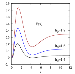
Figure 1: Profiles of $h,q,N$, and $E(x)$ for the positive energy solutions with $Q=kr^{5}/(1+x^{2}e^{x})$.

These solutions describe smooth metric deformations of the flat space. They correspond only to the initial time moment, since later the metric will dynamically evolve, and to determine its temporal evolution will require solving the full system of Hamilton equations. However, the total energy computed at the initial time moment will be the same for all times, and, as can be seen in Fig.1, is positive. Specifically, the energy contained in the sphere or radius $x$ (expressed in $1/m$ units),

$$E(x)=\int_{0}^{x}{\cal E}\,dx,$$ (7.30)

can be negative for small $x$ (if $h_{0}<1$), but the total energy $E(\infty)$ turns out to be always positive and grows when $|h_{0}-1|$ increases. As a result, the energy is positive for smooth, asymptotically flat fields, so that the positivity of their energy in the weak field limit holds in the fully non-linear theory as well.

VII.2 Tachyon branch

For the $h=\frac{1}{2}$ solution in (7.25) one has $N=\frac{1}{2}$ and the two metrics are proportional, $ds_{g}^{2}=\frac{1}{4}\,ds_{f}^{2}$. Even though they are both flat, this solution is quite different from flat space since one now has $E(x)=-x^{3}/8$, which corresponds to the constant and negative energy density. The total energy is negative and infinite.

For small fluctuations around this background one has

$$\Delta=2+\delta,~{}~{}~{}~{}R=\frac{r}{2}+\rho,$$ (7.31)

in addition the momenta $p_{\Delta},p_{R}$ are non-zero but small. Linearizing the constraints (4.12),(4.20) with respect to small $\delta,\rho,p_{\Delta},p_{R}$ then gives the FP constraints (5.5),(5.7), up to the replacement

$$m^{2}\to-\frac{m^{2}}{2}.$$ (7.32)

Therefore, the FP mass becomes imaginary for fluctuations around this background, hence gravitons become tachyons.

One can also construct more general solutions by setting in (7.28) $h_{0}\approx\frac{1}{2}$, in which case $h(x)\to\frac{1}{2}$ as $x\to\infty$. The total energy is always negative and infinite, which can be viewed as an indication of the presence of the ghost. However, if the tachyon branch is completely disjoint from the positive energy branch, then the ghost will be harmless, since it will not be able to affect the positive energy states.

VII.3 Tachyon bubbles.

It is not immediately obvious that the tachyon branch is disjoint from the positive energy branch since there are solutions which interpolate between the two. For these solutions one has $h=1/2$ at the origin but $h\to 1$ at infinity; they can be obtained by choosing in (VII)

$$Q=A\,\Theta(x-x_{0})(x-x_{0})^{p}e^{-x},$$ (7.33)

where $\Theta(x)$ is the step function and $p$ is positive and large enough. Such a choice of $Q$ enforces for $h$ a kink-type behaviour, so that $h=\frac{1}{2}$ for $x<x_{0}$ but $h$ starts to grow for $x>x_{0}$ and $h\to 1$ as $x\to\infty$ (see Fig.2). Solutions thus start from the tachyon phase at the origin but approach flat space at infinity, so that they describe bubbles of the tachyon phase of size $\propto x_{0}$. If $x_{0}$ is large, then the energy $E\propto-x_{0}^{3}$ (see Fig.2).

   

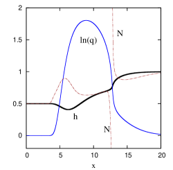
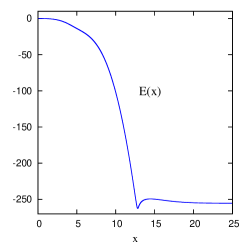
Figure 2: Profiles of $h$ (thick line), $\ln(q)$, $N$, and $E(x)$ for the tachyon bubble solution with $Q=-\Theta(x-3)(x-3)^{8}e^{-x}$.

The bubble 3-metric is regular and asymptotically flat, while the energy is negative. This is embarrassing, since this suggests that the flat space could decay into bubbles. However, a more close inspection reveals that the lapse function $N$ for the bubbles is necessarily singular. Indeed, one has $N={\cal B}/{\cal A}$, but ${\cal A},{\cal B}$ are both negative for $h=\frac{1}{2}$ and become positive for $h=1$, hence each of them vanishes at least once as $h$ interpolates between $\frac{1}{2}$ and $1$. Next, $h$ must cross the value $h=2/3$ at some point where $h^{\prime}>0$. Assuming regular Taylor expansions for $h$ and $q$ and constructing the power-series solution of the constraint (7.20) at this point, it turns out that ${\cal A}$ and ${\cal B}$ are both negative there. Therefore, they must change sign in the region where $h>2/3$. Next, one should check if they can vanish simultaneously. For this, one constructs a power-series solution of the constraint at a point where $x=x_{0}>0$, $h=h_{0}>2/3$, and $q=q_{0}>0$, and one imposes on this solution two additional conditions, ${\cal A}={\cal B}=0$. This yields an algebraic equation for $x_{0},h_{0},q_{0}$, and it turns out that this equation has no solutions. As a result, ${\cal A},{\cal B}$ cannot vanish simultaneously. Therefore, $N$ must have at least one zero and a pole, as shown in Fig.2.

Since $N$ enters the Hamilton equations $\dot{p}_{k}=\{p_{k},H\}_{\rm PB}$, the time derivative of the momenta diverges where $N$ has pole(s). Therefore, the bubble solutions do not describe regular initial data. It follows that the negative energy branch is totally disjoint from the positive energy branch so that it cannot affect the stability of flat space.

The above conclusions apply to the theory with $c_{3}=c_{4}=0$, but the tachyon bubbles can be constructed also for $c_{3}\neq 0$ and $c_{4}\neq 0$. The analysis then becomes more complicated and the above analytical arguments showing that the lapse function $N$ must be singular do not directly apply. Nevertheless, the problem can be tackled numerically, and in all studied cases the lapse $N$ is found to be singular and even worse – when one varies $c_{3}$ and $c_{4}$ or the function $Q(x)$, the lapse $N$ generically starts to exhibit many poles instead of just one pole.

VIII Conclusions – Stability of the theory

To recapitulate the above discussion, the energy in the $s$-sector of the dRGT theory is found to be positive for globally regular and asymptotically flat fields. Besides, there are also solutions of the constraints for which the energy can be negative and even unbounded from below and for which the gravitons behave as tachyons. The negative energies and tachyons can clearly be interpreted as a very bad sign, supporting the viewpoint that the whole theory is sick Deser and Waldron ; *Deser:2013eua; *Deser:2013qza; *Deser:2014hga. However, it is interesting that a different interpretation is also possible, and this we shall now try to advocate.

The main point is that the above global analysis of the constraints shows that their negative energy solutions are always either not globally regular or not asymptotically flat. Therefore, they cannot describe initial data for a decay of the flat space. This indicates that the existence of the negative energies in the theory could actually be harmless since it does not affect the stability of the flat space and of its globally regular deformations.

One can give the following interpretation. Globally regular and asymptotically flat fields constitute the “physical sector” of the theory where the energy is positive and the ghost is absent/bound. This sector is healthy. As for the negative energy states, they belong to different sectors separated from the physical sector by a potential barrier.

One may wonder how high is the potential barrier between the sectors. To estimate, one can compute the energy for an interpolating sequence of fields. For example, fields which fulfill the constraints and satisfy the boundary conditions (7.24) will interpolate between the normal and tachyon branches when the parameter $h_{0}$ in (7.24) varies from $1$ to $1/2$. A numerical evaluation shows that when $h_{0}$ decreases from unit value, the energy rapidly grows (since the function $g$ in the denominator in (7.18) develops a minimum), then it passes through a pole and finally approaches a finite negative value when $h_{0}$ tends to $1/2$. This indicates that the potential barrier between the two sectors is infinitely high.

These arguments support the viewpoint that the physical sector could be protected from the influence of the negative energies. Interestingly, they can be used to argue that the physical sector could be protected also from the waves propagating faster than light, whose existence in the dRGT theory was discovered by using the local analysis of the differential equations Deser and Waldron ; *Deser:2013eua; *Deser:2013qza; *Deser:2014hga. Indeed, it is natural to expect the superluminal waves to coexist with the tachyons, but, as suggested by the above arguments based on the global analysis, the tachyons should decouple to disjoint sectors, as their energy is negative. In other words, it is possible that the superluminal waves cannot develop starting from globally regular and asymptotically flat initial data, in which case they would not appear in the physical sector. Although not a proof, this indicates that the physical sector could be protected from superluminalities and perhaps also from other seemingly non-physical features Deser and Waldron (2014), .

It should be emphasised at the same time that the above interpretation can at best be viewed only as a conjecture, as it is currently based only on the results of the $s$-sector analysis. Of course, these results are suggestive. Indeed, as the ghost is a scalar and can propagate in the $s$-sector, this sector would be the most natural place for the instability to show up. Therefore, its absence in the $s$-sector indicates that it could be absent in all sectors. However, to really prove this would require demonstrating that the energy is positive for arbitrary globally regular deformations of the flat space and that the negative energies totally decouple. Such a demonstration is lacking at present. Therefore, despite the positive evidence mentioned above, the issue of weather the dRGT theory can indeed be considered as a consistent theory remains actually open

It is interesting that within the bigravity generalization of the dRGT theory, where both metrics are dynamical Hassan and Rosen (2012c), the tachyon vacuum in (7.25) is no longer a solution, as it does not fulfill the equations for the second metric Volkov (2012); *Volkov:2013roa. Since there are no tachyons, one does not expect the superluminalities to be present either, and indeed their existence within the bigravity theory has not been reported Deser et al. (2013c). It seems therefore that the bigravity theory could be better defined than the massive gravity since it contains less negative energy solutions, or maybe no such solutions at all. However, a detailed analysis is needed in order to make definite statements.

Appendix A General Relativity Hamiltonian in the s-sector

Let us consider the spherically-symmetric spacetime metric (4.1),

$$ds_{g}^{2} = -N^{2}dt^{2}+\frac{1}{\Delta^{2}}\,(dr+\beta\,dt)^{2}+R^{2}\,(d\vartheta^{2}+\sin^{2}\vartheta d\varphi^{2}),$$ (A.34)

where $N,\beta,\Delta,R$ depend on of $t,r$ . This corresponds to the ADM decomposition (3.1) with the 3-metric

$$\gamma_{ik}\,dx^{i}dx^{k}=\frac{dr^{2}}{\Delta^{2}}+R^{2}\,(d\vartheta^{2}+\sin^{2}\vartheta d\varphi^{2}),$$ (A.35)

and with the shift vector $N^{k}=(N^{r},N^{\vartheta},N^{\varphi})=(\beta,0,0)$. One has $N_{i}=\gamma_{ik}N^{k}=(\beta/\Delta^{2},0,0)$ and $\sqrt{\gamma}=R^{2}/\Delta$, while the curvature scalar for the 3-metric is

$$-\frac{1}{2}\,\sqrt{\gamma}\,R^{(3)}=2\Delta RR^{\prime\prime}+2\Delta^{\prime}RR^{\prime}+\Delta R^{\prime 2}-\frac{1}{\Delta}.$$ (A.36)

Calculating the second fundamental form ($\nabla^{(3)}$ is the covariant derivative with respect to $\gamma_{ik}$),

$$K_{ik}=\frac{1}{2N}(\dot{\gamma}_{ik}-\nabla^{(3)}_{i}N_{k}-\nabla^{(3)}_{k}N_{i}),$$ (A.37)

gives for $K^{i}_{~{}k}=\gamma^{im}K_{mk}$ the only non-trivial components

$$K^{r}_{~{}r}=-\frac{1}{N\Delta}\left(\dot{\Delta}+\Delta\beta^{\prime}-\beta\Delta^{\prime}\right)\,,~{}~{}~{}~{}~{}K^{\vartheta}_{~{}\vartheta}=K^{\varphi}_{~{}\varphi}=\frac{1}{NR}\left(\dot{R}-\beta R^{\prime}\right).$$ (A.38)

The Lagrangian is

$${\cal L} = \frac{1}{2}\,\sqrt{\gamma}N\left(K^{i}_{~{}k}K^{k}_{~{}i}-(K^{k}_{~{}k})^{2}+R^{(3)}\right)-m^{2}{\cal V}$$

$$= \frac{\dot{R}-\beta R^{\prime}}{N^{2}\Delta^{2}}\left(2R\dot{\Delta}-\Delta\dot{R}+\beta\Delta R^{\prime}+2\beta^{\prime}\Delta R-2\beta\Delta^{\prime}R\right)+\frac{1}{2}\,\sqrt{\gamma}R^{(3)}-m^{2}{\cal V}\,.$$

Choosing $\Delta,R$ to be the dynamical variables, their momenta are

$$p_{\Delta} = \frac{\partial{\cal L}}{\partial\dot{\Delta}}=\frac{2R(\dot{R}-\beta R^{\prime})}{N\Delta^{2}}\,,~{}~{}~{}$$

$$p_{R} = \frac{\partial{\cal L}}{\partial\dot{R}}=\frac{2(R\dot{\Delta}-\Delta\dot{R}+\beta^{\prime}\Delta R-\beta\Delta^{\prime}R+\beta\Delta R^{\prime})}{N\Delta^{2}}\,,~{}~{}~{}$$ (A.40)

which relations can be inverted,

$$\dot{\Delta}=\frac{N\Delta^{2}}{2R^{2}}\,(\Delta\,p_{\Delta}+R\,p_{R})+\Delta^{\prime}\beta-\Delta\beta^{\prime}\,,~{}~{}~{}~{}~{}~{}~{}~{}\dot{R}=\frac{N\Delta^{2}}{2R}\,p_{\Delta}+\beta R^{\prime}\,.$$ (A.41)

The Hamiltonian density ${\cal H}=\dot{\Delta}p_{\Delta}+\dot{R}p_{R}-{\cal L}$ reduces to

$${\cal H}=N{\cal H}_{0}+\beta{\cal H}_{r}+m^{2}{\cal V}\,$$ (A.42)

with

$${\cal H}_{0}=\frac{\Delta^{3}}{4R^{2}}\,p_{\Delta}^{2}+\frac{\Delta^{2}}{2R}\,p_{\Delta}p_{R}-\frac{1}{2}\,\sqrt{\gamma}\,R^{(3)},~{}~{}~{}~{}{\cal H}_{r}=\Delta p_{\Delta}^{\prime}+2\Delta^{\prime}p_{\Delta}+R^{\prime}p_{R}\,.$$ (A.43)

This gives rise to Eq.(IV) in the main text. One can equally apply Eqs.(3.5),(3.6) from the main text, according to which

$${\cal H}_{0}=\left.\left.\frac{1}{\sqrt{\gamma}}\,\right(2\pi^{i}_{~{}k}\pi^{k}_{~{}i}-(\pi^{k}_{~{}k})^{2}\right)-\frac{1}{2}\,\sqrt{\gamma}R^{(3)},~{}~{}~{}{\cal H}_{r}=-2\nabla^{(3)}_{i}\pi^{i}_{r}\,,$$ (A.44)

with

$$\pi^{i}_{~{}k}=\frac{1}{2}\,\sqrt{\gamma}\,(K^{i}_{~{}k}-K^{m}_{~{}m}\,\delta^{i}_{k}).$$ (A.45)

Using (A.38),(A.41), the only non-vanishing momenta are

$$\pi^{r}_{~{}r}=-\frac{1}{2}\,\Delta\,p_{\Delta}\,,~{}~{}~{}~{}\pi^{\vartheta}_{~{}\vartheta}=\pi^{\varphi}_{~{}\varphi}=\frac{1}{4}\,R\,p_{R}\,.$$ (A.46)

Inserting this to (A.44) again reproduces Eq.(A.43). The only subtlety is that $\pi^{i}_{~{}k}$ is a tensor density, whose covariant derivative is $\nabla^{(3)}_{i}\pi^{i}_{k}=\sqrt{\gamma}\,\nabla^{(3)}_{i}(\pi^{i}_{k}/\sqrt{\gamma})$, where $\pi^{i}_{k}/\sqrt{\gamma}$ is a tensor whose covariant derivative is computed in the usual way.

Appendix B Metric potential in the s-sector

Let us calculate the potential of the dRGT theory given by Eq.(2.3) in the main text. The first step is to consider the inverse of the spacetime metric (A.34),

$$g^{\mu\nu}=\left(\begin{array}[]{cccc}-{1}/{N^{2}}&{\beta}/{N^{2}}&0&0\\ {\beta}/{N^{2}}&\Delta^{2}-{\beta^{2}}/{N^{2}}&0&0\\ 0&0&{1}/{R^{2}}&0\\ 0&0&0&{1}/{(R^{2}\sin^{2}\vartheta)}\end{array}\right)\,,$$ (B.47)

while the f-metric is

$$ds_{f}^{2}=-dt^{2}+dr^{2}+r^{2}\,(d\vartheta^{2}+\sin^{2}\vartheta d\varphi^{2}),$$ (B.48)

and therefore

$${g^{\mu\sigma}f_{\sigma\nu}}=\left(\begin{array}[]{cccc}1/N^{2}&\beta/N^{2}&0&0\\ -\beta/N^{2}&\Delta^{2}-\beta^{2}/N^{2}&0&0\\ 0&0&r^{2}/R^{2}&0\\ 0&0&0&r^{2}/R^{2}\end{array}\right)\,.$$ (B.49)

Let us apply this first to calculate the potential (2.2) with all higher order terms truncated,

$${\cal U}=\frac{1}{8}\,(H^{\mu}_{~{}\nu}H^{\nu}_{~{}\mu}-(H^{\mu}_{~{}\mu})^{2}),$$ (B.50)

where $H^{\nu}_{\mu}=\delta^{\mu}_{\nu}-g^{\mu\sigma}f_{\sigma\nu}$. With $u\equiv r/R$ one obtains for ${\cal V}=\sqrt{\gamma}N{\cal U}$

$${\cal V}=\left(\frac{3-2u^{2}}{u^{2}}\,\Delta-\frac{u^{4}-6u^{2}+6}{u^{2}\Delta}\right)\frac{r^{2}N}{4}-\left(\frac{\Delta}{u^{2}}+\frac{(3-2u^{2})(\beta^{2}-1)}{u^{2}\Delta}\right)\frac{r^{2}}{4N}\,.$$ (B.51)

Inserting this to ${\cal H}$ in (A.42), one can see that the equations $\partial{\cal H}/\partial N=0$ and $\partial{\cal H}/\partial\beta=0$ admit non-trivial solutions for $N,\beta$, so that no constraints arise.

Next, let us calculate the square root of the matrix (B.49). It can be chosen in the form

$$\boldsymbol{\gamma}^{\mu}_{~{}\nu}=\sqrt{g^{\mu\sigma}f_{\sigma\nu}}=\left(\begin{array}[]{cccc}a&{c}&0&0\\ -c&b&0&0\\ 0&0&u&0\\ 0&0&0&u\end{array}\right)\,,$$ (B.52)

and the conditions $\boldsymbol{\gamma}^{\mu}_{~{}\sigma}\boldsymbol{\gamma}^{\sigma}_{~{}\nu}=g^{\mu\sigma}f_{\sigma\nu}$ then reduce to

$$a^{2}-c^{2} = \frac{1}{N^{2}}\equiv{\rm A},$$

$$b^{2}-c^{2} = \Delta^{2}-\frac{\beta^{2}}{N^{2}}\equiv{\rm B},$$

$$c\,(a+b) = \frac{\beta}{N^{2}}\equiv{\rm C},$$ (B.53)

and also $u^{2}={r^{2}}/{R^{2}}$. These equations can be rewritten as

$$a+b={\rm Y},~{}~{}~{}~{}~{}a-b=\frac{{\rm A}-{\rm B}}{\rm Y},~{}~{}~{}~{}~{}c=\frac{\rm C}{\rm Y}\,,$$ (B.54)

where Y (not to be confused with $Y$ from (4.11)) fulfills

$${\rm Y}^{4}-2({\rm A}+{\rm B}){\rm Y}^{2}+({\rm A}-{\rm B})^{2}-4{\rm C}^{2}=0.$$ (B.55)

Denoting Q$=\Delta/N$, this equation is solved by

$${\rm Y}=\sqrt{{\rm A}+{\rm B}+2{\rm Q}}=\frac{1}{N}\sqrt{(N\Delta+1)^{2}-\beta^{2}}\,,$$ (B.56)

so that

$$a=\frac{{\rm A}+{\rm Q}}{\rm Y},~{}~{}~{}~{}~{}b=\frac{{\rm B}+{\rm Q}}{\rm Y},~{}~{}~{}~{}~{}c=\frac{{\rm C}}{\rm Y},~{}~{}~{}~{}~{}u=\frac{r}{R}\,.$$ (B.57)

Eigenvalues of $\boldsymbol{\gamma}^{\mu}_{~{}\nu}$ are

$$\lambda_{0,1}=\left.\left.\frac{1}{2}\right(a+b\pm\sqrt{(a-b)^{2}-4c^{2}}\right),~{}~{}~{}\lambda_{2}=\lambda_{3}=u,$$ (B.58)

inserting which into (II) gives

$${\cal U}_{1} = a+b+2u={\rm Y}+2u,$$

$${\cal U}_{2} = u(u+2a+2b)+ab+c^{2}=u(u+2{\rm Y})+{\rm Q}\,,$$

$${\cal U}_{3} = u\,(au+bu+2ab+2c^{2})=u(u{\rm Y}+2{\rm Q}),$$

$${\cal U}_{4} = u^{2}(ab+c^{2})=u^{2}{\rm Q}.$$ (B.59)

As a result, the potential ${\cal U}$ in (2.3) is

$${\cal U}=\sum_{k=0}^{4}b_{k}{\cal U}_{k}=P_{0}+P_{1}\,{\rm Y}+P_{2}\,\frac{\Delta}{N}$$ (B.60)

with $P_{m}=b_{m}+2b_{m+1}u+b_{m+2}u^{2}$ for $m=0,1,2$. Multiplying by $\sqrt{\gamma}N=NR^{2}/\Delta$ yields

$${\cal V}=\frac{NR^{2}}{\Delta}\,P_{0}+\frac{R^{2}P_{1}}{\Delta}\,\sqrt{(\Delta N+1)^{2}-\beta^{2}}+R^{2}P_{2}\,,$$ (B.61)

which gives Eq.(4.7) in the main text.

Appendix C Fierz-Pauli limit

Eqs.(A.42),(A.43),(B.61) determine the Hamiltonian ${\cal H}=N{\cal H}_{0}+\beta{\cal H}_{r}+m^{2}{\cal V}$ of the massive gravity theory. Let us consider its weak field limit, where

$$\Delta=1+\delta,~{}~{}~{}~{}~{}~{}R=r+\rho\,,~{}~{}~{}~{}~{}~{}N=1+\nu,$$ (C.1)

with small $\delta$, $\rho$, $\nu$ and where $\beta$, $p_{\Delta}$, $p_{R}$ are also small. One has

$${\cal H}_{0} = \frac{p_{\Delta}^{2}}{4r^{2}}+\frac{p_{\Delta}p_{R}}{2r}+V_{1}+V_{2}+\ldots,~{}~{}~{}~{}{\cal H}_{r}=p_{\Delta}^{\prime}+p_{R}+\ldots,$$

$${\cal V} = \nu(r^{2}\delta-2r\rho)+2r\delta\,\rho-\rho^{2}-\frac{r^{2}}{4}\beta^{2}+\ldots\,,$$ (C.2)

where the dots denote higher order terms, while

$$V_{1} = (2r(\delta+\rho^{\prime}))^{\prime}\,,~{}~{}~{}~{}~{}V_{2}=2\rho\,\delta^{\prime}-\rho^{\prime 2}-\delta^{2}+\mbox{total derivative}.$$ (C.3)

It is worth noting that both for the generic potential ${\cal V}$ in (B.51) and for the dRGT potential (B.61) the quadratic terms in the expansion in (C) are the same.

Dropping the total derivatives and keeping only the quadratic terms, the Hamiltonian density ${\cal H}=N{\cal H}_{0}+\beta{\cal H}_{r}+m^{2}{\cal V}$ reduces to

$${\cal H}_{\rm FP} = \frac{p_{\Delta}^{2}}{4r^{2}}+\frac{p_{\Delta}p_{R}}{2r}+V_{2}+\nu\,V_{1}+\beta(p_{\Delta}^{\prime}+p_{R})$$ (C.4)

$$+ m^{2}\left(\nu(r^{2}\delta-2r\rho)+2r\delta\,\rho-\rho^{2}-\frac{r^{2}}{4}\beta^{2}\right).$$

Varying this with respect to $\nu$ gives the constraint,

$${\cal C}_{\rm FP}\equiv\frac{\partial{\cal H}_{\rm FP}}{\partial\nu}=(2r(\delta+\rho^{\prime}))^{\prime}+m^{2}(r^{2}\delta-2r\rho)=0,$$ (C.5)

while varying with respect to $\beta$ gives the equation

$$p_{\Delta}^{\prime}+p_{R}-\frac{m^{2}r^{2}}{2}\,\beta=0\,,$$ (C.6)

so that

$$\beta=\frac{2(p_{\Delta}^{\prime}+p_{R})}{m^{2}r^{2}}\,.$$ (C.7)

Injecting this into ${\cal H}_{\rm FP}$, the result is

$${\cal H}_{\rm FP}={\cal E}_{\rm FP}+\nu\,{\cal C}_{\rm FP}\,,$$ (C.8)

where

$${\cal E}_{\rm FP}(\pi)=\frac{p_{\Delta}^{2}}{4r^{2}}+\frac{p_{\Delta}p_{R}}{2r}+\frac{(p_{\Delta}^{\prime}+p_{R})^{2}}{m^{2}r^{2}}+2\rho\,\delta^{\prime}-\rho^{\prime 2}-\delta^{2}+m^{2}(2r\delta\rho-\rho^{2}).$$ (C.9)

Commuting ${\cal C}_{\rm FP}$ with the Hamiltonian $H_{\rm FP}=\int_{0}^{\infty}{\cal H}_{\rm FP}dr$ gives the second constraint,

$${\cal S}_{\rm FP}=\{{\cal C}_{\rm FP},H_{\rm FP}\}=\frac{m^{2}}{2}\,(rp_{R}-p_{\Delta})-(p_{\Delta}^{\prime}+p_{R})^{\prime}=0\,.$$ (C.10)

These expressions for ${\cal C}_{\rm PF}$, ${\cal H}_{\rm PF}$, ${\cal S}_{\rm PF}$ give rise to Eqs.(5.4)–(5.7) for the FP energy and constraints in the main text. The same expressions can also be obtained by inserting the linearised

$$\pi^{i}_{k}={\rm diag}\left[-\frac{p_{\Delta}}{2},\frac{p_{R}}{4},\frac{p_{R}}{4}\right],~{}~{}~{}~{}h^{i}_{k}={\rm diag}\left[-2\delta,\frac{2\rho}{r},\frac{2\rho}{r}\right],~{}~{}~{}~{}$$ (C.11)

into Eqs.(3.19), (3.22), (3.23) with $f_{ik}dx^{i}dx^{k}=dr^{2}+r^{2}d\Omega^{2}$.

It is instructive to derive Eqs.(C.5),(C.8),(C.9) once again via expanding the expressions (4.12),(4.20),(4.16) for the energy ${\cal E}_{0}$ and constraints ${\cal C,S}$ obtained in Section V. Expanding the constraints (4.12),(4.20) gives

$$0={\cal C}={\cal C}^{(1)}+{\cal C}^{(2)}+\mbox{cubic and higher order terms},$$ (C.12)

with ${\cal C}^{(1)}={\cal C}_{\rm FP}$ and

$${\cal C}^{(2)}={\cal E}_{\rm FP}-\frac{(p_{\Delta}^{\prime}+p_{R})^{2}}{2m^{2}r^{2}}+2\left((\rho+r\delta)\rho^{\prime}\right)^{\prime}+m^{2}[(c_{3}-2)\rho(\rho-2r\delta)-r^{2}\delta^{2}]),$$ (C.13)

and also

$$0={\cal S}={\cal S}_{\rm FP}+\mbox{quadratic and higher order terms}.$$ (C.14)

One can see that the linear terms in the expansions (C.12),(C.14) agree with (5.5),(5.7). Let us now expand the energy density (4.16). Dropping the total derivative,

$${\cal E}_{0}={\cal E}^{(1)}_{0}+{\cal E}^{(2)}_{0}+\mbox{cubic and higher order terms},$$

with ${\cal E}^{(1)}_{0}=-2\,{\cal C}_{\rm FP}$ and

$${\cal E}^{(2)}_{0} = -\frac{p_{\Delta}^{2}}{4r^{2}}-\frac{p_{\Delta}p_{R}}{2r}+\rho^{\prime 2}-2\rho\delta^{\prime}-2r\rho^{\prime}\delta^{\prime}+2\delta^{2}$$

$$+ m^{2}[(5-2c_{3})\rho^{2}+4\,(c_{3}-3)\,r\rho\,\delta+3r^{2}\delta^{2}].$$

Comparing with (C.9), one can see that ${\cal E}_{0}$ looks actually quite different from ${\cal E}_{\rm FP}$, so that one may wonder how the two expressions could agree with each other. However, they completely agree when the constraints are imposed up to the second order terms. Indeed, according to Eq.(4.15) one has ${\cal H}={\cal E}_{0}+(N+1/\Delta)\,{\cal C}$. Expanding this around flat space and comparing with (C.8) gives the relation

$${\cal E}_{\rm FP}={\cal E}^{(1)}_{0}+{\cal E}^{(2)}_{0}+2\,({\cal C}^{(1)}+{\cal C}^{(2)})-\delta\,{\cal C}^{(1)}\,,$$ (C.16)

which can be directly verified. The constraint ${\cal C}=0$ implies that ${\cal C}^{(1)}+{\cal C}^{(2)}=0$, up to higher order terms, hence ${\cal C}^{(1)}=-{\cal C}^{(2)}$, and therefore the term $\delta\,{\cal C}^{(1)}$ is actually cubic in fields. As a result, the last three terms on the right in (C.16) do not contribute in the quadratic approximation, so that ${\cal E}_{\rm FP}={\cal E}^{(1)}_{0}+{\cal E}^{(2)}_{0}={\cal E}_{0}$.

Appendix D Positivity of the Fierz-Pauli energy

It is instructive to verify that the FP energy is indeed positive, which is not immediately obvious. The FP energy is

$$E_{\rm FP}=\int{\cal H}_{\rm FP}(\pi_{ik})\,d^{3}x+\int{\cal H}_{\rm FP}(h_{ik})\,d^{3}x\,$$ (D.1)

with ${\cal H}_{\rm FP}(\pi_{ik})$ and ${\cal H}_{\rm FP}(h_{ik})$ defined by Eqs.(3.21) and (3.22) in the main text, where $h_{ik}$ and $\pi_{ik}$ should fulfill the constraints (3.19) and (3.23). Let us consider the Fourrier expansion,

$$\pi_{ik}({\bf x})=\frac{1}{(2\pi)^{3/2}}\int\Pi_{ik}({\bf k})e^{i{\bf kx}}d^{3}k\,,~{}~{}~{}$$ (D.2)

with $\Pi_{ik}({\bf k})=\Pi_{ik}^{\ast}(-{\bf k})$, the star denoting complex conjugation. One has

$$\int{\cal H}_{\rm FP}(\pi_{ik})\,d^{3}x=\frac{1}{(2\pi)^{3/2}}\int{\cal E}({\bf k})d^{3}k\,,$$ (D.3)

where

$${\cal E}({\bf k})=2\sum_{i,k}|\Pi_{ik}|^{2}-|\sum_{s}\Pi_{ss}|^{2}+\frac{4}{m^{2}}\sum_{i}\left|\sum_{s}\Pi_{is}k^{s}\right|^{2},$$ (D.4)

with $\Pi_{ik}\equiv\Pi_{ik}({\bf k})$. The constraint (3.23) requires

$$m^{2}\sum_{s}\Pi_{ss}-2\sum_{i,s}k^{i}k^{s}\Pi_{is}=0.$$ (D.5)

The symmetric tensor $\Pi_{ik}({\bf k})$ can be expanded in the tensor basis,

$$\Pi_{ik}({\bf k})=\sum_{a=1}^{6}\phi_{a}({\bf k})\Pi^{(a)}_{ik},$$ (D.6)

where the tensors $\Pi^{(a)}_{ik}$ can be chosen to describe two spin-2 tensor harmonics, two spin-1 vector harmonics, and two scalar modes. Aligning the third coordinate axis along vector ${\bf k}$, the tensor modes are traceless and orthogonal to ${\bf k}$,

$$\Pi^{(1)}_{ik}=\frac{1}{\sqrt{2}}\begin{pmatrix}1&0&0\\ 0&-1&0\\ 0&0&0\\ \end{pmatrix},~{}~{}~{}~{}\Pi^{(2)}_{ik}=\frac{1}{\sqrt{2}}\begin{pmatrix}0&1&0\\ 1&0&0\\ 0&0&0\\ \end{pmatrix},$$ (D.7)

the vector modes are

$$\Pi^{(3)}_{ik}=\frac{1}{\sqrt{2}}\begin{pmatrix}0&0&1\\ 0&0&0\\ 1&0&0\\ \end{pmatrix},~{}~{}~{}~{}\Pi^{(4)}_{ik}=\frac{1}{\sqrt{2}}\begin{pmatrix}0&0&0\\ 0&0&1\\ 0&1&0\\ \end{pmatrix},$$ (D.8)

while the scalar modes

$$\Pi^{(5)}_{ik}=\frac{1}{\sqrt{6}}\,{\rm diag}[1,1,-2],~{}~{}~{}~{}\Pi^{(6)}_{ik}=\frac{1}{\sqrt{3}}\,\delta_{ik}\,,$$ (D.9)

so that

$$\sum_{ik}\Pi^{(a)}_{ik}\Pi^{(b)}_{ki}=\delta_{ab}.$$ (D.10)

Inserting (D.6) to (D.4), ${\cal E}({\bf k})$ becomes

$${\cal E}({\bf k})=2\sum_{a=1}^{5}|\phi_{a}|^{2}-|\phi_{6}|^{2}+2s^{2}(|\phi_{3}|^{2}+|\phi_{4}|^{2})+\left.\left.\frac{4s^{2}}{3}\right|\sqrt{2}\,\phi_{5}-\phi_{6}\right|^{2}\,,$$ (D.11)

with $s^{2}={\bf k}^{2}/m^{2}$. This expression is not positive definite. However, the constraint (D.5) imposes the relation between the two scalar modes,

$$\frac{2\sqrt{2}\,s^{2}}{\sqrt{3}}\,\phi_{5}+\sqrt{3}\left(1-\frac{2s^{2}}{{3}}\right)\phi_{6}=0,$$ (D.12)

which removes one of the two scalars. In view of this the energy becomes

$${\cal E}({\bf k})=2(|\phi_{1}|^{2}+|\phi_{2}|^{2})+2(1+s^{2})(|\phi_{3}|^{2}+|\phi_{4}|^{2})+\frac{9}{4s^{4}}|\phi_{6}|^{2}\,,$$ (D.13)

therefore $\int{\cal H}_{\rm FP}(\pi_{ik})\,d^{3}x\geq 0$. Similarly one shows that $\int{\cal H}_{\rm FP}(h_{ik})\,d^{3}x\geq 0$.

Appendix E Poisson brackets

Some care is needed when computing the Poisson brackets (see, for example, Khoury et al. (2012)). Let us denote by $q_{k}=(\Delta,R)$ and $p_{k}=(p_{\Delta},p_{R})$ the phase space coordinates and their momenta, they depend on time and on the radial coordinate $r$. Consider a function on the phase space,

$${\cal F}=(q_{k},q_{k}^{\prime},q_{k}^{\prime\prime},\ldots q_{k}^{(M)},p_{k},p_{k}^{\prime},p_{k}^{\prime\prime},\ldots p_{k}^{(M)},r)\,,$$ (E.1)

where the primes denote derivatives with respect to $r$, while $M$ is the order of the highest derivative. One considers the functional

$$F=\int_{0}^{\infty}f(r){\cal F}\,dr\,,$$ (E.2)

where $f$ is a smoothening function, which is assumed to vanish fast enough for $r\to 0,\infty$ in order that one could integrate by parts and always drop the boundary terms. The variation of $F$ is

$$\delta F=\int f(r)\sum_{k}\left(\frac{\partial{\cal F}}{\partial q_{k}}\,\delta q_{k}+\ldots+\frac{\partial{\cal F}}{\partial q^{(M)}_{k}}\,\delta q^{(M)}_{k}+\frac{\partial{\cal F}}{\partial p_{k}}\,\delta p_{k}+\ldots+\frac{\partial{\cal F}}{\partial p^{(M)}_{k}}\,\delta p^{(M)}_{k}\right)dr$$ (E.3)

and integrating by parts,

$$\delta F=\int dr\sum_{k}\left(f\frac{\partial{\cal F}}{\partial q_{k}}-\left(f\frac{\partial{\cal F}}{\partial q^{\prime}_{k}}\right)^{\prime}+\ldots+(-1)^{M}\left(f\frac{\partial{\cal F}}{\partial q^{(M)}_{k}}\right)^{(M)}\right)\delta q_{k}$$

$$+\int dr\sum_{k}\left(f\frac{\partial{\cal F}}{\partial p_{k}}-\left(f\frac{\partial{\cal F}}{\partial p^{\prime}_{k}}\right)^{\prime}+\ldots+(-1)^{M}\left(f\frac{\partial{\cal F}}{\partial p^{(M)}_{k}}\right)^{(M)}\right)\delta p_{k}\,.$$ (E.4)

Therefore, the functional derivatives are

$$\frac{\delta F}{\delta q_{k}}=f\frac{\partial{\cal F}}{\partial q_{k}}-\left(f\frac{\partial{\cal F}}{\partial q^{\prime}_{k}}\right)^{\prime}+\ldots+(-1)^{M}\left(f\frac{\partial{\cal F}}{\partial q^{(M)}_{k}}\right)^{(M)}\,,$$

$$\frac{\delta F}{\delta p_{k}}=f\frac{\partial{\cal F}}{\partial p_{k}}-\left(f\frac{\partial{\cal F}}{\partial p^{\prime}_{k}}\right)^{\prime}+\ldots+(-1)^{M}\left(f\frac{\partial{\cal F}}{\partial p^{(M)}_{k}}\right)^{(M)}\,.$$ (E.5)

Let us consider another function on the phase space,

$${\cal G}(q_{k},q_{k}^{\prime},q_{k}^{\prime\prime},\ldots q_{k}^{(M)},p_{k},p_{k}^{\prime},p_{k}^{\prime\prime},\ldots p_{k}^{(M)},r)\,,$$ (E.6)

whose smoothened version is

$$G=\int_{0}^{\infty}g(r){\cal G}\,dr\,,$$ (E.7)

with another smoothening function $g(r)$. The functional derivatives are

$$\frac{\delta G}{\delta q_{k}}=g\frac{\partial{\cal G}}{\partial q_{k}}-\left(g\frac{\partial{\cal G}}{\partial q^{\prime}_{k}}\right)^{\prime}+\ldots+(-1)^{M}\left(g\frac{\partial{\cal G}}{\partial q^{(M)}_{k}}\right)^{(M)}\,,$$

$$\frac{\delta G}{\delta p_{k}}=g\frac{\partial{\cal G}}{\partial p_{k}}-\left(g\frac{\partial{\cal G}}{\partial p^{\prime}_{k}}\right)^{\prime}+\ldots+(-1)^{M}\left(g\frac{\partial{\cal G}}{\partial p^{(M)}_{k}}\right)^{(M)}\,.$$ (E.8)

The Poisson bracket is defined as

$$\{F,G\}_{\rm PB} = \int_{0}^{\infty}dr\sum_{k}\left(\frac{\delta F}{\delta q_{k}}\frac{\delta G}{\delta p_{k}}-\frac{\delta F}{\delta p_{k}}\frac{\delta G}{\delta q_{k}}\right)$$ (E.9)

$$\equiv \int_{0}^{\infty}\int_{0}^{\infty}dr\,ds\,f(r)g(s)\,\{{\cal F}(r),{\cal G}(s)\}_{\rm PB}.$$

To compute the integrand in the first line here one uses the definitions (E),(E), while the passage to the second line is achieved by inserting the delta-functions. For the analysis in the main body of the paper it is sufficient to calculate only the first line in (E.9). This only requires implementing the definitions (E),(E), which can be efficiently done with MAPLE, say. For example, for ${\cal H}_{0}$ and ${\cal H}_{r}$ defined in (IV) one obtains

$$\{H_{0},H_{0}\}_{\rm PB} = \int_{0}^{\infty}dr(fg^{\prime}-f^{\prime}g)\,\Delta^{2}{\cal H}_{r}\,,~{}$$

$$\{H_{0},H_{r}\}_{\rm PB} = \int_{0}^{\infty}drf\left(g{\cal H}_{0}\right)^{\prime}\,,$$

$$\{H_{r},H_{r}\}_{\rm PB} = \int_{0}^{\infty}dr(fg^{\prime}-f^{\prime}g){\cal H}_{r}\,.$$ (E.10)

Inserting here the delta functions gives the $t,r$ part of the diffeomorphism algebra Khoury et al. (2012),

$$\{{\cal H}_{0}(r),{\cal H}_{0}(s)\}_{\rm PB} = {\cal H}^{r}(r)\partial_{r}\,\delta(r-s)-{\cal H}^{r}(s)\partial_{s}\,\delta(r-s),$$

$$\{{\cal H}_{0}(r),{\cal H}_{r}(s)\}_{\rm PB} = {\cal H}_{0}(s)\partial_{r}\,\delta(r-s),$$

$$\{{\cal H}_{r}(r),{\cal H}_{r}(s)\}_{\rm PB} = {\cal H}_{r}(r)\partial_{r}\,\delta(r-s)-{\cal H}_{r}(s)\partial_{s}\,\delta(r-s).$$ (E.11)

Next, when computing the commutator of the constraint ${\cal C}(r)$ with itself one obtains

$$\{C,C\}_{\rm PB}=\int_{0}^{\infty}dr(fg^{\prime}-f^{\prime}g)\,\frac{\Delta^{2}}{Y}\,{\cal C}\,,\\$$

with $Y$ from (4.11), from where it follows that $\{{\cal C}(r_{1}),{\cal C}(r_{2})\}_{\rm PB}=0$ if ${\cal C}=0$. Similarly, the secondary constraint ${\cal S}(r)=\{{\cal C}(r),H\}$ is obtained by computing $\{C,H\}_{\rm PB}$, which yields and expression of the form

$$\int_{0}^{\infty}dr(fA_{0}+f^{\prime}A_{1}+\ldots+A_{M}f^{(M)})\,.\\$$

Integrating by parts brings this to

$$\int_{0}^{\infty}dr\left(A_{0}-(A_{1})^{\prime}+\ldots+(-1)^{M}(A_{M})^{(M)}\right)f\,,$$ (E.12)

and setting $f=g=1$ the integrand gives ${\cal S}$.

References

- Riess et al. (1998) A. Riess et al., Astron.Journ. 116, 1009 (1998).
- Perlmutter et al. (1999) S. Perlmutter et al., Astrophys.Journ. 517, 565 (1999).
- de Rham et al. (2011) C. de Rham, G. Gabadadze, and A. Tolley, Phys.Rev.Lett. 106, 231101 (2011).
- Hinterbichler (2012) K. Hinterbichler, Rev.Mod.Phys. 84, 671 (2012).
- de Rham (2014) C. de Rham, (2014), arXiv:1401.4173 .
- Hassan and Rosen (2012a) S. Hassan and R. A. Rosen, Phys.Rev.Lett. 108, 041101 (2012a).
- Hassan and Rosen (2012b) S. Hassan and R. A. Rosen, JHEP 1204, 123 (2012b).
- Kluson (2012) J. Kluson, Phys.Rev. D86, 044024 (2012).
- Comelli et al. (2012) D. Comelli, M. Crisostomi, F. Nesti, and L. Pilo, Phys.Rev. D86, 101502 (2012).
- Comelli et al. (2013) D. Comelli, F. Nesti, and L. Pilo, (2013), arXiv:1305.0236 .
- De Felice et al. (2012) A. De Felice, E. Gumrukcuoglu, and S. Mukohyama, Phys.Rev.Lett. 109, 171101 (2012).
- Fasiello and Tolley (2013) M. Fasiello and A. J. Tolley, JCAP 1312, 002 (2013).
- Chamseddine and Mukhanov (2013) A. H. Chamseddine and V. Mukhanov, JHEP 1303, 092 (2013).
- Arnowitt et al. (1962) R. L. Arnowitt, S. Deser, and C. W. Misner, in Gravitation: An Introduction to Current Research, edited by Louis Witten (Wiley, 1962) Chap. 7, pp. 227–265, gr-qc/0405109 .
- (15) S. Deser and A. Waldron, Phys.Rev.Lett. 110, 111101.
- Deser et al. (2013a) S. Deser, K. Izumi, Y. Ong, and A. Waldron, Phys.Lett. B726, 544 (2013a).
- Deser et al. (2013b) S. Deser, K. Izumi, Y. Ong, and A. Waldron, (2013b), arXiv:1312.1115 .
- Deser et al. (2014) S. Deser, M. Sandora, A. Waldron, and G. Zahariade, (2014), arXiv:1408.0561 .
- Volkov (2014) M. S. Volkov, Phys.Rev. D90, 024028 (2014).
- Fierz and Pauli (1939) M. Fierz and W. Pauli, Proc.Roy.Soc.Lond. A173, 211 (1939).
- Boulware and Deser (1972) D. Boulware and S. Deser, Phys.Rev. D6, 3368 (1972).
- Regge and Teitelboim (1974) T. Regge and C. Teitelboim, Annals Phys. 88, 286 (1974).
- Khoury et al. (2012) J. Khoury, G. E. Miller, and A. J. Tolley, Phys.Rev. D85, 084002 (2012).
- Van Nieuwenhuizen (1973) P. Van Nieuwenhuizen, Nucl.Phys. B60, 478 (1973).
- Unruh (1976) W. Unruh, Phys.Rev. D14, 870 (1976).
- Kuchar (1994) K. V. Kuchar, Phys.Rev. D50, 3961 (1994).
- Deser and Waldron (2014) S. Deser and A. Waldron, Phys.Rev. D89, 027503 (2014).
- Note (1) It is argued in Deser and Waldron ; *Deser:2013eua; *Deser:2013qza; *Deser:2014hga that the dRGT theory admits not only superluminal waves but also closed causal curves, a least in the case where the two metric have different signatures. However, since should be complex-valued in that case, it is not quite clear if one can consistently set the two metric signatures to be not the same.
- Note (2) A ghost-type instability in the dRGT theory with flat reference metric was detected for perturbations around the de Sitter space De Felice et al. (2012); *Fasiello:2013woa; *Chamseddine:2013lid. However, it is unclear if this invalidates the whole theory, as there are infinitely many inequivalent versions of de Sitter solution in the theory Volkov (2013), only one of them being considered in De Felice et al. (2012); *Fasiello:2013woa; *Chamseddine:2013lid.
- Hassan and Rosen (2012c) S. Hassan and R. A. Rosen, JHEP 1202, 126 (2012c).
- Volkov (2012) M. S. Volkov, JHEP 1201, 035 (2012).
- Volkov (2013) M. S. Volkov, Class.Quant.Grav. 30, 184009 (2013).
- Deser et al. (2013c) S. Deser, M. Sandora, and A. Waldron, Phys.Rev. D88, 081501 (2013c).