On the Minimal Revision Problem of Specification Automata

Abstract

As robots are being integrated into our daily lives, it becomes necessary to provide guarantees on the safe and provably correct operation. Such guarantees can be provided using automata theoretic task and mission planning where the requirements are expressed as temporal logic specifications. However, in real-life scenarios, it is to be expected that not all user task requirements can be realized by the robot. In such cases, the robot must provide feedback to the user on why it cannot accomplish a given task. Moreover, the robot should indicate what tasks it can accomplish which are as “close” as possible to the initial user intent. This paper establishes that the latter problem, which is referred to as the minimal specification revision problem, is NP complete. A heuristic algorithm is presented that can compute good approximations to the Minimal Revision Problem (MRP) in polynomial time. The experimental study of the algorithm demonstrates that in most problem instances the heuristic algorithm actually returns the optimal solution. Finally, some cases where the algorithm does not return the optimal solution are presented.

I Introduction

As robots become mechanically more capable, they are going to be more and more integrated into our daily lives. Non-expert users will have to communicate with the robots in a natural language setting and request a robot or a team of robots to accomplish complicated tasks. Therefore, we need methods that can capture the high-level user requirements, solve the planning problem and map the solution to low level continuous control actions. In addition, such frameworks must come with mathematical guarantees of safe and correct operation for the whole system and not just the high level planning or the low level continuous control.

Linear Temporal Logic (LTL) (see Clarke et al. 1999) can provide the mathematical framework that can bridge the gap between

1. natural language and high-level planning algorithms (e.g., Kress-Gazit et al. 2008; Dzifcak et al. 2009), and

2. high-level planning algorithms and control (e.g., Fainekos et al. 2009; Karaman et al. 2008; Bhatia et al. 2010; Wongpiromsarn et al. 2010; Roy et al. 2011).

LTL has been utilized as a specification language in a wide range of robotics applications. For a good coverage of the current research directions, the reader is referred to Fainekos et al. 2009; Kress-Gazit et al. 2009; Karaman et al. 2008; Kloetzer and Belta 2010; Bhatia et al. 2010; Wongpiromsarn et al. 2010; Roy et al. 2011; Bobadilla et al. 2011; Ulusoy et al. 2011; Lacerda and Lima 2011; LaViers et al. 2011; Filippidis et al. 2012 and the references therein.

For instance, in Fainekos et al. 2009, the authors present a framework for motion planning of a single mobile robot with second order dynamics. The problem of reactive planning and distributed controller synthesis for multiple robots is presented in Kress-Gazit et al. 2009 for a fragment of LTL (Generalized Reactivity 1 (GR1)). The authors in Wongpiromsarn et al. 2010 present a method for incremental planning when the specifications are provided in the GR1 fragment of LTL. The papers Kloetzer and Belta 2010; Ulusoy et al. 2011 address the problem of centralized control of multiple robots where the specifications are provided as LTL formulas. An application of LTL planning methods to humanoid robot dancing is presented in LaViers et al. 2011. In Karaman et al. 2008, the authors convert the LTL planning problem into Mixed Integer Linear Programming (MILP) or Mixed Integer Quadratic Programming (MIQP) problems. The use of sampling-based methods for solving the LTL motion planning problem is explored in Bhatia et al. 2010. All the previous applications assume that the robots are autonomous agents with full control over their actions. An interesting different approach is taken in Bobadilla et al. 2011 where the agents move uncontrollably in the environment and the controller opens and closes gates in the environment.

All the previous methods are based on the assumption that the LTL planning problem has a feasible solution. However, in real-life scenarios, it is to be expected that not all complex task requirements can be realized by a robot or a team of robots. In such failure cases, the robot needs to provide feedback to the non-expert user on why the specification failed. Furthermore, it would be desirable that the robot proposes a number of plans that can be realized by the robot and which are as “close” as possible to the initial user intent. Then, the user would be able to understand what are the limitations of the robot and, also, he/she would be able to choose among a number of possible feasible plans.

In Fainekos 2011, we made the first steps towards solving the debugging (i.e., why the planning failed) and revision (i.e., what the robot can actually do) problems for automata theoretic LTL planning (Giacomo and Vardi 1999). We remark that a large number of robotic applications, e.g., Fainekos et al. 2009; Kloetzer and Belta 2010; Bhatia et al. 2010; Bobadilla et al. 2011; Ulusoy et al. 2011 and LaViers et al. 2011, are utilizing this particular LTL planning method.

In the follow-up paper Kim et al. 2012, we studied the theoretical foundations of the specification revision problem when both the system and the specification can be represented by $\omega$-automata (Buchi 1960). In particular, we focused on the Minimal Revision Problem (MRP), i.e., finding the “closest” satisfiable specification to the initial specification, and we proved that the problem is NP-complete even when severely restricting the search space. Furthermore, we presented an encoding of MRP as a satisfiability problem and we demonstrated experimentally that we can quickly get the exact solution to MRP for small problem instances.

In Kim and Fainekos 2012, we revisited MRP and we presented a heuristic algorithm that can approximately solve MRP in polynomial time. We experimentally established that the heuristic algorithm almost always returns the optimal solution on random problem instances and on LTL planning scenarios from our previous work. Furthermore, we demonstrated that we can quickly return a solution to the MRP problem on large problem instances. Finally, we provided examples where the algorithm is guaranteed not to return the optimal solution.

This paper is an extension of the preliminary work by Kim et al. 2012 and Kim and Fainekos 2012. In this extended journal version, we present a unified view of the theory alongside with the proofs that were omitted in the aforementioned papers. The class of specifications that can be handled by our framework has been extended as well. The framework that was presented in Kim et al. 2012 was geared towards robotic motion planning specifications as presented in Fainekos et al. 2009. In addition, we prove that the heuristic algorithm that we presented in Kim and Fainekos 2012 has a constant approximation ratio only on a specific class of graphs. Furthermore, we have included several running examples to enhance the readability of the paper as well as more case studies to demonstrate the feasibility of the framework. On the other hand, we have excluded some details on the satisfiability encoding of the MRP problem which can be found in Kim et al. 2012.

II Problem Formulation

In this paper, we work with discrete abstractions (Finite State Machines) of the continuous robotic control system (Fainekos et al. 2009). This is a common practice in approaches that hierarchically decompose the control synthesis problem into high level discrete planning synthesis and low level continuous feedback controller composition (e.g., Fainekos et al. 2009; Kress-Gazit et al. 2009; LaViers et al. 2011; Kloetzer and Belta 2010; Ulusoy et al. 2011). Each state of the Finite State Machine (FSM) $\mathcal{T}$ is labeled by a number of symbols from a set $\Pi=\{\pi_{0},$ $\pi_{1},$ $\dots,$ $\pi_{n}\}$ that represent regions in the configuration space (see LaValle 2006 or Choset et al. 2005) of the robot or, more generally, actions that can be performed by the robot. The control requirements for such a system can be posed using specification automata $\mathcal{B}$ with Büchi acceptance conditions (see Buchi 1960) also known as $\omega$-automata.

The following example presents a scenario for motion planning of a mobile robot.

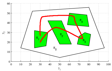
Figure 1: The simple environment of Example 1 along with a low speed mobile robot trajectory that satisfies the specification.

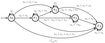
Figure 2: The specification automaton $\mathcal{B}_{m}$ of Example 1.

Example 1 (Robot Motion Planning).

We consider a mobile robot which operates in a planar environment. The continuous state variable $x(t)$ models the internal dynamics of the robot whereas only its position $y(t)$ is observed. In this paper, we will consider a 2nd order model of the motion of a planar robot (dynamic model):

$$\dot{x}_{1}(t) =x_{2}(t), \;x_{1}(t)\in\mathbb{R}^{2},\;x_{1}(0)\in X_{1,0}$$

$$\dot{x}_{2}(t) =u(t), \;x_{2}(t)\in\mathbb{R}^{2},\;x_{2}(0)=0,\;u(t)\in U$$

$$y(t) =x_{1}(t).$$

The robot is moving in a convex polygonal environment $\pi_{0}$ with four areas of interest denoted by $\pi_{1},\pi_{2},\pi_{3},\pi_{4}$ (see Fig. 1). Initially, the robot is placed somewhere in the region labeled by $\pi_{1}$. The robot must accomplish the task: “Stay always in $\pi_{0}$ and visit area $\pi_{2}$, then area $\pi_{3}$, then area $\pi_{4}$ and, finally, return to and stay in region $\pi_{1}$ while avoiding area $\pi_{2}$,” which is captured by the specification automaton in Fig. 2.

In Fainekos et al. 2009, we developed a hierarchical framework for motion planning for dynamic models of robots. The hierarchy consists of a high level logic planner that solves the motion planning problem for a kinematic model of the robot, e.g.,

$$\dot{z}(t) =u(t), \;z(t)\in\mathbb{R}^{2},\;z(0)\in Z_{0}$$

$$y^{\prime}(t) =z(t).$$

Then, the resulting hybrid controller is utilized for the design of an approximate tracking controller for the dynamic model. Since the tracking is approximate, the sets $\pi$ need to be modified (see Fig. 3 for an example) depending on the maximum speed of the robot so that the controller has a guaranteed tracking performance. For example, in Fig. 3, the regions that now must be visited are the contracted yellow regions, while the regions to be avoided are the expanded red regions. However, the set modification might make the specification unrealizable, e.g., in Fig. 3 the robot cannot move from $\pi_{4}$ to $\pi_{1}$ while avoiding $\pi_{2}$, even though the specification can be realized on the workspace of the robot that the user perceives. In this case, the user is entirely left in the dark as of why the specification failed and, more importantly, on what actually the system can achieve under these new constraints. This is especially important since the low level controller synthesis details should be hidden from the end user. $\bigtriangleup$

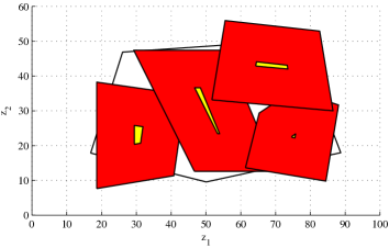
Figure 3: The modified environment of Fig. 1 under large bounds on the permissible acceleration $U$. The red regions indicate areas that should be avoided in order to satisfy $\neg\pi_{i}$ while the yellow regions indicate areas that should be visited in order to satisfy $\pi_{i}$.

The next example presents a typical scenario for task planning with two agents.

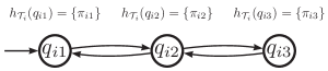
Figure 4: Simple FSM model $\mathcal{T}_{i}$ of an autonomous agent. Each state $j$ of the FSM $i$ is labeled by an atomic proposition $\pi_{ij}$.

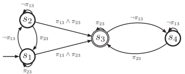
Figure 5: The specification automaton of Example 2.

Example 2 (Multi-Agent Planning).

We consider two autonomous agents whose independent actions can be modeled using an FSM as in Fig. 4. In this example, each state $q_{i}$ represents a location $i$. In order to construct a simple example, we assume that at each discrete time instance only one agent can move. Alternatively, we can think of these agents as being objects moved around by a mobile manipulator and that the manipulator can move only one object at a time. This means that the state of both objects can be described by the asynchronous composition of the two state machines $\mathcal{T}_{1}$ and $\mathcal{T}_{2}$. The asynchronous composition results in a FSM $\mathcal{T}$ with 9 states where each state $(q_{1i},q_{2j})$ is labeled by $h_{\mathcal{T}}(q_{1i},q_{2j})=h_{\mathcal{T}_{1}}(q_{1i})\cup h_{\mathcal{T}_{2}}(q_{2j})$.

The system must accomplish the task: “Object 2 should be placed in Location 3 after Object 1 is placed in Location 3”. Note that this requirement could be used to enforce that Object 2 is going to be positioned on top of Object 1 at the end of the system execution. However, the requirement permits temporary placing Object 2 in Location 3 before Object 1 is placed in Location 3. This should be allowed for problems where a temporary reposition of the objects is necessary. Now, let’s assume that the aforementioned task is just a part from a long list or requirements which also include the task: “Always, Object 1 should not be in Location 3 until Object 2 moves in Location 3”.

These are informal requirements and in order to give them mathematical meaning we will have to use a formal language. In Linear Temporal Logic (LTL) (see Clarke et al. 1999), the requirements become: F($\pi_{13}$ $\wedge$ F$\pi_{23}$) and G(($\neg$$\pi_{13}$)$\,\mathcal{U}$$\pi_{23}$). We remark that the conjunction of these two requirements is actually a satisfiable specification (even though the requirements appear conflicting) and the corresponding specification automaton is presented in Fig. 5. The specification remains satisfiable because the semantics of the logic permit both objects to be place in Location 3 at the same time (see transitions on label $\pi_{13}\wedge\pi_{23}$ from states $s_{1}$ and $s_{2}$ to state $s_{3}$).

However, there is no trajectory of the FSM $\mathcal{T}$ that will satisfy the specification. Recall that the model does not allow for simultaneous transitions of the two objects. Again, the user does not know why the specification failed and, more importantly, on what actually the system can achieve that is “close” to the initial user intent. $\bigtriangleup$

When a specification $\mathcal{B}$ is not satisfiable on a particular system $\mathcal{T}$, then the current motion planning and control synthesis methods (e.g., Fainekos et al. 2009; Kloetzer and Belta 2010; LaViers et al. 2011) based on automata theoretic concepts (see Giacomo and Vardi 1999) simply return that the specification is not satisfiable without any other user feedback. In such cases, we would like to be able to solve the following problem and provide feedback to the user.

Problem 1 (Minimal Revision Problem (MRP)).

Given a system $\mathcal{T}$ and a specification automaton $\mathcal{B}$, if the specification $\mathcal{B}$ cannot be satisfied on $\mathcal{T}$, then find the “closest” specification $\mathcal{B}^{\prime}$ to $\mathcal{B}$ which can be satisfied on $\mathcal{T}$.

Problem 1 was first introduced in Fainekos 2011 for Linear Temporal Logic (LTL) specifications. In Fainekos 2011, we provided solutions to the debugging and (not minimal) revision problems and we demonstrated that we can easily get a minimal revision of the specification when the discrete controller synthesis phase fails due to unreachable states in the system.

Assumption 1.

All the states on $\mathcal{T}$ are reachable.

In Kim et al. 2012, we introduced a notion of distance on a restricted space of specification automata and, then, we were able to demonstrate that MRP is in NP-complete even on that restricted search space of possible solutions. Since brute force search is prohibitive for any reasonably sized problem, we presented an encoding of MRP as a satisfiability problem. Nevertheless, even when utilizing state of the art satisfiability solvers, the size of the systems that we could handle remained small (single robot scenarios in medium complexity environments).

In Kim and Fainekos 2012, we provided an approximation algorithm for MRP. The algorithm is based on Dijkstra’s single-source shortest path algorithm (see Cormen et al. 2001), which can be regarded both as a greedy and a dynamic programming algorithm (see Sniedovich 2006). We demonstrated through numerical experiments that not only the algorithm returns an optimal solution in various scenarios, but also that it outperforms in computation time our satisfiability based solution. Then, we presented some scenarios where the algorithm is guaranteed not to return the optimal solution.

Contributions: In this paper, we define the MRP problem and we provide the proof that MRP is NP-complete even when restricting the search space (e.g., Problem 2). Then, we provide an approximation algorithm for MRP and theoretically establish the upper bound of the algorithm for a special case. Furthermore, we show that for our heuristic algorithm a constant approximation ratio cannot be established, in general. We also present experimental results of the scalability of our framework and establish some experimental approximation bounds on random problem instances. Finally, in order to improve the paper presentation, we also provide multiple examples that have not been published before.

III Preliminaries

In this section, we review some basic results on the automata theoretic planning and the specification revision problem from Fainekos et al. 2009; Fainekos 2011.

Throughout the paper, we will use the notation $\mathcal{P}(A)$ for representing the powerset of a set $A$, i.e., $\mathcal{P}(A)=\{B\;|\;B\subseteq A\}$. Clearly, it includes $\emptyset$ and $A$ itself. We also define the set difference as $A\setminus B=\{x\in A\;|\;x\notin B\}$.

III-A Constructing Discrete Controllers

We assume that the combined actions of the robot/team of robots and their operating environment can be represented using an FSM.

Definition 1 (FSM).

A Finite State Machine is a tuple $\mathcal{T}=(Q,Q_{0},\rightarrow_{\mathcal{T}},h_{\mathcal{T}},\Pi)$ where:

• $Q$ is a set of states;

• $Q_{0}\subseteq Q$ is the set of possible initial states;

• $\rightarrow_{\mathcal{T}}\subseteq Q\times Q$ is the transition relation; and,

• $h_{\mathcal{T}}:Q\rightarrow\mathcal{P}(\Pi)$ maps each state $q$ to the set of atomic propositions that are true on $q$.

We define a path on the FSM to be a sequence of states and a trace to be the corresponding sequence of sets of propositions. Formally, a path is a function $p:\mathbb{N}\rightarrow Q$ such that for each $i\in\mathbb{N}$ we have $p(i)\rightarrow_{\mathcal{T}}p(i+1)$ and the corresponding trace is the function composition $\bar{p}=h_{\mathcal{T}}\circ p:\mathbb{N}\rightarrow\mathcal{P}(\Pi)$. The language $\mathcal{L}(\mathcal{T})$ of $\mathcal{T}$ consists of all possible traces.

Example 3.

For the two agent system in Example 2, a path would be $(q_{11},q_{21})(q_{11},q_{22})(q_{12},q_{22})\ldots$ and the corresponding trace would be $\{\pi_{11},\pi_{21}\}\{\pi_{11},\pi_{22}\}\{\pi_{12},\pi_{22}\}\ldots$.

In this work, we are interested in the $\omega$-automata that will impose certain requirements on the traces of $\mathcal{T}$. Omega automata differ from the classic finite automata in that they accept infinite strings (traces of $\mathcal{T}$ in our case).

Definition 2.

A automaton is a tuple $\mathcal{B}=(S_{\mathcal{B}},s_{0}^{\mathcal{B}},\Omega,\rightarrow_{\mathcal{B}},F_{\mathcal{B}})$ where:

• $S_{\mathcal{B}}$ is a finite set of states;

• $s_{0}^{\mathcal{B}}$ is the initial state;

• $\Omega$ is an input alphabet;

• $\rightarrow_{\mathcal{B}}\subseteq S_{\mathcal{B}}\times\Omega\times S_{\mathcal{B}}$ is a transition relation; and

• $F_{\mathcal{B}}\subseteq S_{\mathcal{B}}$ is a set of final states.

We also write $s\stackrel{{\scriptstyle l}}{{\rightarrow}}_{\mathcal{B}}s^{\prime}$ instead of $(s,l,s^{\prime})\in\rightarrow_{\mathcal{B}}$. A specification automaton is an automaton with Büchi acceptance condition where the input alphabet is the powerset of the labels of the system $\mathcal{T}$, i.e., $\Omega=\mathcal{P}(\Pi)$.

A run $r$ of a specification automaton $\mathcal{B}$ is a sequence of states $r:\mathbb{N}\rightarrow S_{\mathcal{B}}$ that occurs under an input trace $\bar{p}$ taking values in $\Omega=\mathcal{P}(\Pi)$. That is, for $i=0$ we have $r(0)=s_{0}^{\mathcal{B}}$ and for all $i\geq 0$ we have $r(i)\stackrel{{\scriptstyle\bar{p}(i)}}{{\rightarrow}}_{\mathcal{B}}r(i+1)$. Let $\lim(\cdot)$ be the function that returns the set of states that are encountered infinitely often in the run $r$ of $\mathcal{B}$. Then, a run $r$ of an automaton $\mathcal{B}$ over an infinite trace $\bar{p}$ is accepting if and only if $\lim(r)\cap F_{\mathcal{B}}\neq\emptyset$. This is called a Büchi acceptance condition. Finally, we define the language $\mathcal{L}(\mathcal{B})$ of $\mathcal{B}$ to be the set of all traces $\bar{p}$ that have a run that is accepted by $\mathcal{B}$.

Even though the definition of specification automata (Def. 2) only uses sets of atomic propositions for labeling transitions, it is convenient for the user to read and write specification automata with propositional formulas on the transitions. The popular translation tools from LTL to automata, e.g., Gastin and Oddoux (2001), label the transitions with propositional formulas in Disjunctive Normal Form (DNF). A DNF formula on a transition of a specification automaton can represent multiple transitions between two states. In the subsequent sections, we will be making the following simplifying assumption on the structure of the specification automata that we consider.

Assumption 2.

All the propositional formulas that appear on the transitions of a specification automaton are in Disjunctive Normal Form (DNF). That is, for any two states $s_{1}$, $s_{2}$ of an automaton $\mathcal{B}$, we represent the propositional formula that labels the corresponding transition by $\Phi_{\mathcal{B}}(s_{1},s_{2})=\bigvee_{i\in D_{s_{1}s_{2}}}\bigwedge_{j\in C^{i}_{s_{1}s_{2}}}\psi_{ij}$ for some appropriate set of indices $D_{s_{1}s_{2}}$ and $C^{i}_{s_{1}s_{2}}$. Here, $\psi_{ij}$ is a literal which is $\pi$ or $\neg\pi$ for some $\pi\in\Pi$. Finally, we assume that when any subformula in $\Phi_{\mathcal{B}}(s_{1},s_{2})$ is a tautology or a contradiction, then it is replaced by $\top$ (true) or $\bot$ (false), respectively.

The last assumption is necessary in order to avoid converting a contradiciton like $\pi\wedge\neg\pi$ into a satisfiable formula (see Sec. IV). We remark that the Assumption 2 does not restrict the scope of this work. Any propositional formula can be converted in DNF where any negation symbol appears in front of an atomic proposition.

Example 4.

Let us consider the specification automaton in Fig. 5. The propositional formulas over the set of atomic propositions $\Pi$ are shorthands for the subsets of $\Pi$ that would label the corresponding transitions. For example, the label $\pi_{13}\wedge\pi_{23}$ over the edge $(s_{2},s_{3})$ succinctly represents all the transitions $(s_{2},l,s_{3})$ such that $\{\pi_{13},\pi_{23}\}\subseteq l\subseteq\Pi$. On the other hand, the label $\neg\pi_{13}$ over the edge $(s_{1},s_{2})$ succinctly represents all the transitions $(s_{1},l,s_{2})$ such that $l\subseteq\Pi$ and $\pi_{13}\not\in l$. On input trace $\{\pi_{11},\pi_{21}\}\{\pi_{11},\pi_{22}\}\{\pi_{12},\pi_{22}\}\ldots$ the corresponding run would be $s_{1}s_{2}s_{2}s_{2}\ldots$. $\bigtriangleup$

In brief, our goal is to generate paths on $\mathcal{T}$ that satisfy the specification $\mathcal{B}_{\mathbf{s}}$. In automata theoretic terms, we want to find the subset of the language $\mathcal{L}(\mathcal{T})$ which also belongs to the language $\mathcal{L}(\mathcal{B}_{\mathbf{s}})$. This subset is simply the intersection of the two languages $\mathcal{L}(\mathcal{T})\cap\mathcal{L}(\mathcal{B}_{\mathbf{s}})$ and it can be constructed by taking the product $\mathcal{T}\times\mathcal{B}_{\mathbf{s}}$ of the FSM $\mathcal{T}$ and the specification automaton $\mathcal{B}_{\mathbf{s}}$. Informally, the automaton $\mathcal{B}_{\mathbf{s}}$ restricts the behavior of the system $\mathcal{T}$ by permitting only certain acceptable transitions. Then, given an initial state in the FSM $\mathcal{T}$, we can choose a particular trace from $\mathcal{L}(\mathcal{T})\cap\mathcal{L}(\mathcal{B}_{\mathbf{s}})$ according to a preferred criterion.

Definition 3.

The product automaton $\mathcal{A}=\mathcal{T}\times\mathcal{B}_{\mathbf{s}}$ is the automaton $\mathcal{A}=(S_{\mathcal{A}},s_{0}^{\mathcal{A}},\mathcal{P}(\Pi),\rightarrow_{\mathcal{A}},F_{\mathcal{A}})$ where:

• $\mathcal{S}_{\mathcal{A}}=Q\times S_{\mathcal{B}_{\mathbf{s}}}$,

• $s_{0}^{\mathcal{A}}=\{(q_{0},s_{0}^{\mathcal{B}_{\mathbf{s}}})\;|\;q_{0}\in Q_{0}\}$,

• $\rightarrow_{\mathcal{A}}\subseteq S_{\mathcal{A}}\times\mathcal{P}(\Pi)\times S_{\mathcal{A}}$ s.t. $(q_{i},s_{i})\stackrel{{\scriptstyle l}}{{\rightarrow}}_{\mathcal{A}}(q_{j},s_{j})$ iff $q_{i}\rightarrow_{\mathcal{T}}q_{j}$ and $s_{i}\stackrel{{\scriptstyle l}}{{\rightarrow}}_{\mathcal{B}_{\mathbf{s}}}s_{j}$ with $l=h_{\mathcal{T}}(q_{j})$, and

• $F_{\mathcal{A}}=Q\times F_{\mathcal{B}}$ is the set of accepting states.

Note that $\mathcal{L}(\mathcal{A})=\mathcal{L}(\mathcal{T})\cap\mathcal{L}(\mathcal{B}_{\mathbf{s}})$. We say that $\mathcal{B}_{\mathbf{s}}$ is satisfiable on $\mathcal{T}$ if $\mathcal{L}(\mathcal{A})\neq\emptyset$. Moreover, finding a satisfying path on $\mathcal{T}\times\mathcal{B}_{\mathbf{s}}$ is an easy algorithmic problem (see Clarke et al. 1999). First, we convert automaton $\mathcal{T}\times\mathcal{B}_{\mathbf{s}}$ to a directed graph and, then, we find the strongly connected components (SCC) in that graph.

If at least one SCC that contains a final state is reachable from an initial state, then there exist accepting (infinite) runs on $\mathcal{T}\times\mathcal{B}_{\mathbf{s}}$ that have a finite representation. Each such run consists of two parts: prefix: a part that is executed only once (from an initial state to a final state) and, lasso: a part that is repeated infinitely (from a final state back to itself). Note that if no final state is reachable from the initial or if no final state is within an SCC, then the language $\mathcal{L}(\mathcal{A})$ is empty and, hence, the high level synthesis problem does not have a solution. Namely, the synthesis phase has failed and we cannot find a system behavior that satisfies the specification.

Example 5.

The product automaton of Example 2 has 36 states and 240 number of transitions. However, no final state is reachable from the initial state. $\bigtriangleup$

IV The Specification Revision Problem

Intuitively, a revised specification is one that can be satisfied on the discrete abstraction of the workspace or the configuration space of the robot. In order to search for a minimal revision, we need first to define an ordering relation on automata as well as a distance function between automata. Similar to the case of LTL formulas in Fainekos 2011, we do not want to consider the “space” of all possible automata, but rather the “space” of specification automata which are semantically close to the initial specification automaton $\mathcal{B}_{\mathbf{s}}$. The later will imply that we remain close to the initial intention of the designer. We propose that this space consists of all the automata that can be derived from $\mathcal{B}_{\mathbf{s}}$ by relaxing the restrictions for transitioning from one state to another. In other words, we introduce possible transitions between two states of the specification automaton.

Example 6.

Consider the specification automaton $\mathcal{B}_{\mathbf{s}}$ and the automaton $\mathcal{B}_{1}$ in Fig. 6. The transition relations of the two automata are defined as:

$$\rightarrow_{\mathcal{B}_{\mathbf{s}}}= \stackrel{{\scriptstyle 0\xrightarrow{\neg\pi_{0}}_{\mathcal{B}_{\mathbf{s}}}0}}{{\overbrace{\{(0,l,0)\;|\;l\subseteq\Pi\text{ and }\pi_{0}\not\in l\}}}}\cup\stackrel{{\scriptstyle 0\xrightarrow{\pi_{2}}_{\mathcal{B}_{\mathbf{s}}}0}}{{\overbrace{\{(0,l,0)\;|\;\{\pi_{2}\}\subseteq l\subseteq\Pi\}}}}\cup\stackrel{{\scriptstyle 0\xrightarrow{\neg\pi_{0}\wedge\pi_{1}}_{\mathcal{B}_{\mathbf{s}}}1}}{{\overbrace{\{(0,\{\pi_{1}\},1),(0,\{\pi_{1},\pi_{2}\},1)\}}}}\cup$$

$$\cup\stackrel{{\scriptstyle 1\xrightarrow{\neg\pi_{0}}_{\mathcal{B}_{\mathbf{s}}}1}}{{\overbrace{\{(1,l,1)\;|\;l\subseteq\Pi\text{ and }\pi_{0}\not\in l\}}}}\cup\stackrel{{\scriptstyle 1\xrightarrow{\neg\pi_{0}\wedge\pi_{2}}_{\mathcal{B}_{\mathbf{s}}}2}}{{\overbrace{\{(1,\{\pi_{2}\},2),(1,\{\pi_{1},\pi_{2}\},2)\}}}}\cup\stackrel{{\scriptstyle 0\xrightarrow{\neg\pi_{0}\wedge\pi_{1}\wedge\pi_{2}}_{\mathcal{B}_{\mathbf{s}}}2}}{{\overbrace{\{(0,\{\pi_{1},\pi_{2}\},2)\}}}}\cup$$

$$\cup\stackrel{{\scriptstyle 2\xrightarrow{\neg\pi_{0}}_{\mathcal{B}_{\mathbf{s}}}2}}{{\overbrace{\{(2,l,2)\;|\;l\subseteq\Pi\text{ and }\pi_{0}\not\in l\}}}}$$

$$\rightarrow_{\mathcal{B}_{1}}= \stackrel{{\scriptstyle 0\xrightarrow{\top}_{\mathcal{B}_{1}}0}}{{\overbrace{\{(0,l,0)\;|\;l\subseteq\Pi\}}}}\cup\stackrel{{\scriptstyle 0\xrightarrow{\neg\pi_{0}\wedge\pi_{1}}_{\mathcal{B}_{1}}1}}{{\overbrace{\{(0,\{\pi_{1}\},1),(0,\{\pi_{1},\pi_{2}\},1)\}}}}\cup\stackrel{{\scriptstyle 1\xrightarrow{\top}_{\mathcal{B}_{1}}1}}{{\overbrace{\{(1,l,1)\;|\;l\subseteq\Pi\}}}}\cup\stackrel{{\scriptstyle 1\xrightarrow{\neg\pi_{0}\wedge\pi_{2}}_{\mathcal{B}_{1}}2}}{{\overbrace{\{(1,\{\pi_{2}\},2),(1,\{\pi_{1},\pi_{2}\},2)\}}}}\cup$$

$$\cup\stackrel{{\scriptstyle 1\xrightarrow{\pi_{2}}_{\mathcal{B}_{1}}2}}{{\overbrace{\{(1,l,2)\;|\;\{\pi_{2}\}\subseteq l\subseteq\Pi\}}}}\cup\stackrel{{\scriptstyle 2\xrightarrow{\neg\pi_{0}}_{\mathcal{B}_{1}}2}}{{\overbrace{\{(2,l,2)\;|\;l\subseteq\Pi\text{ and }\pi_{0}\not\in l\}}}}$$

and, hence, $\rightarrow_{\mathcal{B}_{\mathbf{s}}}\subset\rightarrow_{\mathcal{B}_{1}}$. In other words, any transition allowed by $\mathcal{B}_{\mathbf{s}}$ is also allowed by $\mathcal{B}_{1}$ and, thus, any trace accepted by $\mathcal{B}_{\mathbf{s}}$ is also accepted $\mathcal{B}_{1}$. If we view this from the perspective of the specification, then this means that the specification imposes less restrictions or that the specification automaton $\mathcal{B}_{1}$ is a relaxed specification with respect to $\mathcal{B}_{\mathbf{s}}$.

As the previous example indicated, specification relaxation could be defined as the subset relation between the transition relations of the specification automata. However, this is not sufficient from the perspective of user requirements. For instance, consider again Example 6. The transition $\leavevmode\hbox to11.37pt{\vbox to11.37pt{\text{[drawing]}}}\xrightarrow{\neg\pi_{0}\wedge\pi_{2}}_{\mathcal{B}_{\mathbf{s}}}\leavevmode\hbox to11.37pt{\vbox to11.37pt{\text{[drawing]}}}$ could be relaxed as $\leavevmode\hbox to11.37pt{\vbox to11.37pt{\text{[drawing]}}}\xrightarrow{(\neg\pi_{0}\wedge\pi_{2})\vee\pi_{3}}_{\mathcal{B}_{\mathbf{s}}}\leavevmode\hbox to11.37pt{\vbox to11.37pt{\text{[drawing]}}}$. A relevant relaxation from the user perspective should be removing either of the constraints $\neg\pi_{0}$ or $\pi_{2}$ rather than introducing a new requirement $\pi_{3}$. Introducing $\pi_{3}$ may implicitly relaxe both constraints $\neg\pi_{0}$ and $\pi_{2}$ in certain contexts. However, our goal in this paper is to find a minimal relaxation.

In Sec. III, we indicated that a transition relation could be compactly represented using a proposition formula $\Phi_{\mathcal{B}}(s_{1},s_{2})=\bigvee_{i\in D_{s_{1}s_{2}}}\bigwedge_{j\in C^{i}_{s_{1}s_{2}}}\psi_{ij}$ in DNF. Given a pair of states $(s_{1},s_{2})$ and a set of indices $\hat{D}_{s_{1}s_{2}}$, $\hat{C}^{i}_{s_{1}s_{2}}$, we define a substitution $\theta$ as

$$\theta(s_{1},s_{2},\psi_{ij})=\left\{\begin{array}[]{ll}\top&\text{ if }i\in\hat{D}_{s_{1}s_{2}}\text{ and }j\in\hat{C}^{i}_{s_{1}s_{2}}\\ \psi_{ij}&\text{ otherwise }\\ \end{array}\right.$$

That is, a substitution only relaxes the constraints on the possible transitions between two automaton states.

Definition 4 (Relaxation).

Let $\mathcal{B}_{1}=(S_{\mathcal{B}_{1}}$, $s_{0}^{\mathcal{B}_{1}}$, $\Omega$, $\rightarrow_{\mathcal{B}_{1}}$, $F_{\mathcal{B}_{1}})$ and $\mathcal{B}_{2}=(S_{\mathcal{B}_{2}},s_{0}^{\mathcal{B}_{2}},\Omega,\rightarrow_{\mathcal{B}_{2}},F_{\mathcal{B}_{2}})$ be two Büchi automata. Then, we say that $\mathcal{B}_{2}$ is a relaxation of $\mathcal{B}_{1}$ and we write $\mathcal{B}_{1}\preceq\mathcal{B}_{2}$ if and only if (1) $S_{\mathcal{B}_{1}}=S_{\mathcal{B}_{2}}=S$, (2) $s_{0}^{\mathcal{B}_{1}}=s_{0}^{\mathcal{B}_{2}}$, (3) $F_{\mathcal{B}_{1}}=F_{\mathcal{B}_{2}}$ and (4) there exists a substitution $\theta$ such that for all $(s,s^{\prime})\in S\times S$, we have $\Phi_{\mathcal{B}_{2}}(s,s^{\prime})\equiv\bigvee_{i\in D_{ss^{\prime}}}\bigwedge_{j\in C^{i}_{ss^{\prime}}}\theta(s,s^{\prime},\psi_{ij})$ when $\Phi_{\mathcal{B}_{1}}(s,s^{\prime})=\bigvee_{i\in D_{ss^{\prime}}}\bigwedge_{j\in C^{i}_{ss^{\prime}}}\psi_{ij}$.

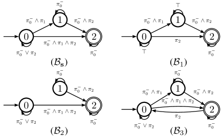
Figure 6: Example 7. $\mathcal{B}_{\mathbf{s}}$: the initial specification automaton, here $\pi_{0}^{-}\equiv\neg\pi_{0}$; $\mathcal{B}_{\mathbf{s}}\preceq\mathcal{B}_{1}$; $\mathcal{B}_{\mathbf{s}}\parallel\mathcal{B}_{2}$; $\mathcal{B}_{\mathbf{s}}\parallel\mathcal{B}_{3}$.

In Def. 4, when defining $\Phi_{\mathcal{B}_{2}}(s,s^{\prime})$, we use the equivalence relation $\equiv$ rather then equality $=$ in order to highlight that in the resulting DNF formula no constant $\top$ appears in a subformula. The only case where $\top$ can appear is when $\Phi_{\mathcal{B}_{2}}(s,s^{\prime})\equiv\top$. We remark that if $\mathcal{B}_{1}\preceq\mathcal{B}_{2}$, then $\mathcal{L}(\mathcal{B}_{1})\subseteq\mathcal{L}(\mathcal{B}_{2})$ since the relaxed automaton allows more behaviors to occur. If two automata $\mathcal{B}_{1}$ and $\mathcal{B}_{2}$ cannot be compared under relation $\preceq$, then we write $\mathcal{B}_{1}\parallel\mathcal{B}_{2}$. The intuition behind the ordering relation in Def. 4 is better explained by an example.

Example 7 (Continuing from Example 6).

Consider the specification automaton $\mathcal{B}_{\mathbf{s}}$ and the automata $\mathcal{B}_{1}$-$\mathcal{B}_{3}$ in Fig. 6. Definition 4 specifies that the two automata must have transitions between exactly the same states. Moreover, if the propositional formula that labels a transition between the same pair of states on the two automata differs, then the propositional formula on the relaxed automaton must be derived by the corresponding label of the original automaton by removing literals. The latter means that we have relaxed the constraints that permit a transition on the specification automaton.

By visual inspection of $\mathcal{B}_{\mathbf{s}}$ and $\mathcal{B}_{1}$ in Fig. 6, we see that $\mathcal{B}_{\mathbf{s}}\preceq\mathcal{B}_{1}$. For example, the transition $\leavevmode\hbox to11.37pt{\vbox to11.37pt{\text{[drawing]}}}\xrightarrow{\pi_{2}}_{\mathcal{B}_{1}}\leavevmode\hbox to11.37pt{\vbox to11.37pt{\text{[drawing]}}}$ is derived from $\leavevmode\hbox to11.37pt{\vbox to11.37pt{\text{[drawing]}}}\xrightarrow{\neg\pi_{0}\wedge\pi_{1}\wedge\pi_{2}}_{\mathcal{B}_{\mathbf{s}}}\leavevmode\hbox to11.37pt{\vbox to11.37pt{\text{[drawing]}}}$ by replacing the literals $\neg\pi_{0}$ and $\pi_{1}$ with $\top$. Similarly, we have $\mathcal{B}_{\mathbf{s}}\parallel\mathcal{B}_{2}$ since $\Phi_{\mathcal{B}_{\mathbf{s}}}(0,1)=\neg\pi_{0}\wedge\pi_{1}$ and $\Phi_{\mathcal{B}_{2}}(0,1)=\bot$, i.e., we have removed a transition between two states. We also have $\mathcal{B}_{\mathbf{s}}\parallel\mathcal{B}_{3}$ since $\Phi_{\mathcal{B}_{\mathbf{s}}}(2,0)=\bot$ and $\Phi_{\mathcal{B}_{3}}(2,0)=\pi_{2}$, i.e., we have added a transition between two states. $\bigtriangleup$

We remark that we restrict the space of relaxed specification automata to all automata that have the same number of states, the same initial state, and the same set of final states for computational reasons. Namely, under these restrictions, we can convert the specification revision problem into a graph search problem. Otherwise, the graph would have to me mutated by adding and/or removing states.

We can now define the set of automata over which we will search for a minimal solution that has nonempty intersection with the system.

Definition 5.

Given a system $\mathcal{T}$ and a specification automaton $\mathcal{B}_{\mathbf{s}}$, the set of valid relaxations of $\mathcal{B}_{\mathbf{s}}$ is defined as $\mathfrak{R}(\mathcal{B}_{\mathbf{s}},\mathcal{T})=\{\mathcal{B}\;|\;\mathcal{B}_{\mathbf{s}}\preceq\mathcal{B}\mbox{ and }\mathcal{L}(\mathcal{T}\times\mathcal{B})\neq\emptyset\}.$

We can now search for a minimal solution in the set $\mathfrak{R}(\mathcal{B}_{\mathbf{s}},\mathcal{T})$. That is, we can search for some $\mathcal{B}\in\mathfrak{R}(\mathcal{B}_{\mathbf{s}},\mathcal{T})$ such that if for any other $\mathcal{B}^{\prime}\in\mathfrak{R}(\mathcal{B}_{\mathbf{s}},\mathcal{T})$, we have $\mathcal{B}^{\prime}\preceq\mathcal{B}$, then $\mathcal{L}(\mathcal{B})=\mathcal{L}(\mathcal{B}^{\prime})$. However, this does not imply that a minimal solution semantically is minimal structurally as well. In other words, it could be the case that $\mathcal{B}_{1}$ and $\mathcal{B}_{2}$ are minimal relaxations of some $\mathcal{B}_{\mathbf{s}}$, but $\mathcal{B}_{1}\parallel\mathcal{B}_{2}$ and, moreover, $\mathcal{B}_{1}$ requires the modification of only one transition while $\mathcal{B}_{2}$ requires the modification of two transitions. Therefore, we must define a metric on the set $\mathfrak{R}(\mathcal{B}_{\mathbf{s}},\mathcal{T})$, which accounts for the number of changes from the initial specification automaton $\mathcal{B}_{\mathbf{s}}$.

Definition 6.

(Distance) Given a system $\mathcal{T}$ and a specification automaton $\mathcal{B}_{\mathbf{s}}$, we define the distance of any $\mathcal{B}\in\mathfrak{R}(\mathcal{B}_{\mathbf{s}},\mathcal{T})$ that results from $\mathcal{B}_{\mathbf{s}}$ under substitution $\theta$ to be $\mathbf{dist}_{\mathcal{B}_{\mathbf{s}}}(\mathcal{B})$ = $\sum_{(s,s^{\prime})\in E_{\mathcal{B}_{\mathbf{s}}}}\sum_{i\in\hat{D}_{ss^{\prime}}}|\hat{C}^{i}_{ss^{\prime}}|$ where $|\cdot|$ is the cardinality of the set.

We remark that given two relaxations $\mathcal{B}_{1}$ and $\mathcal{B}_{2}$ of some $\mathcal{B}_{\mathbf{s}}$ where $\mathcal{B}_{1}\preceq\mathcal{B}_{2}$, but $\mathcal{B}_{2}\npreceq\mathcal{B}_{1}$, then $\mathbf{dist}_{\mathcal{B}_{\mathbf{s}}}(\mathcal{B}_{1})\leq\mathbf{dist}_{\mathcal{B}_{\mathbf{s}}}(\mathcal{B}_{2})$.

Therefore, Problem 1 can be restated as:

Problem 2.

Given a system $\mathcal{T}$ and a specification automaton $\mathcal{B}_{\mathbf{s}}$ such that $\mathcal{L}(\mathcal{T}\times\mathcal{B}_{\mathbf{s}})=\emptyset$, find $\mathcal{B}\in\arg\min\{\mathbf{dist}_{\mathcal{B}_{\mathbf{s}}}(\mathcal{B}^{\prime})\;|\;\mathcal{B}^{\prime}\in\mathfrak{R}(\mathcal{B}_{\mathbf{s}},\mathcal{T})\}$.

IV-A Minimal Revision as a Graph Search Problem

In order to solve Problem 2, we construct a directed labeled graph $G_{\mathcal{A}}$ from the product automaton $\mathcal{A}=\mathcal{T}\times\mathcal{B}_{\mathbf{s}}$. The edges of $G_{\mathcal{A}}$ are labeled by a set of atomic propositions which if removed from the corresponding transition on $\mathcal{B}_{\mathbf{s}}$, they will enable the transition on $\mathcal{A}$. The overall problem then becomes one of finding the least number of atomic propositions to be removed in order for the product graph to have an accepting run. Next, we provide the formal definition of the graph $G_{\mathcal{A}}$ which corresponds to a product automaton $\mathcal{A}$ while considering the effect of revisions.

To formally define the graph search problem, we will need some additional notation. We first create two new sets of symbols from the set of atomic propositions $\Pi$:

• $\Pi^{-}=\{\pi^{-}\;|\;\pi\in\Pi\}$.

• $\widetilde{\Pi}=\{l^{+}\cup l^{-}\;|\;l^{+}\subseteq\Pi\text{ and }l^{-}\subseteq\xi_{S}(\Pi\setminus l^{+})\}$.

Given a transition between two states $s_{1}$ and $s_{2}$ of some $\mathcal{B}$ and a formula in DNF on the transition, we denote:

• $\xi_{l}(\psi)$ = $\pi$ if $\psi=\pi$, and $\pi^{-}$ if $\psi=\neg\pi$.

• $\xi_{S}(l)=\{\pi^{-}\;|\;\pi\in l\}$ where $l\subseteq\Pi$.

Now, we can introduce the following notation. We define

• the set $E_{\mathcal{B}}\subseteq S_{\mathcal{B}}^{2}$, such that $(s,s^{\prime})\in E_{\mathcal{B}}$ iff $\exists l\in\mathcal{P}(\Pi)$ , $s\stackrel{{\scriptstyle l}}{{\rightarrow}}_{\mathcal{B}}s^{\prime}$; and,

• the function $\lambda_{\mathcal{B}}(s_{1},s_{2})=\{\{\xi_{l}(\psi_{ij})\;|\;j\in C^{i}_{s_{1}s_{2}}\}\;|\;i\in D_{s_{1}s_{2}}\}$ as a transition function that maps a pair of states to the set of symbols that represent conjunctive clause.

That is, if $(s,s^{\prime})\in E_{\mathcal{B}}$, then $\exists l\in\mathcal{P}(\Pi)$. $s\stackrel{{\scriptstyle l}}{{\rightarrow}}_{\mathcal{B}}s^{\prime}$; and if $(s,s^{\prime})\not\in E_{\mathcal{B}}$, then $\lambda_{\mathcal{B}}(s,s^{\prime})=\emptyset$. Also, if $\lambda_{\mathcal{B}}(s,s^{\prime})\neq\emptyset$, then $\forall l\in\lambda_{\mathcal{B}}(s,s^{\prime})$ . $l\subseteq\mathcal{P}(\widetilde{\Pi})$.

Example 8.

Consider a set $\Pi=\{\pi_{0},\pi_{1}\}$. Then, $\widetilde{\Pi}=\{\emptyset,\{\pi_{0}\},\{\pi^{-}_{0}\},\{\pi_{1}\},\{\pi^{-}_{1}\},\{\pi_{0},\pi^{-}_{1}\},\{\pi^{-}_{0},\pi_{1}\},\Pi,\Pi^{-}\}$. Given a transition $(s_{1},s_{2})$ of $\mathcal{B}$ and same $\Pi$, consider $\Phi_{\mathcal{B}}(s_{1},s_{2})=\neg\pi_{0}\vee\pi_{1}$ on that transition. Then, $\lambda_{\mathcal{B}}(s_{1},s_{2})=\{\{\pi^{-}_{0}\},\{\pi_{1}\}\}$. If $\Phi_{\mathcal{B}}(s_{1},s_{2})=\neg\pi_{0}\wedge\pi_{1}$, then $\lambda_{\mathcal{B}}(s_{1},s_{2})=\{\{\pi^{-}_{0},\pi_{1}\}\}$.

Definition 7.

Given a system $\mathcal{T}$ and a specification automaton $\mathcal{B}_{\mathbf{s}}$, we define the graph $G_{\mathcal{A}}=(V,E,v_{s},V_{f},\overline{\Pi},\Lambda_{S})$, which corresponds to the product $\mathcal{A}=\mathcal{T}\times\mathcal{B}_{\mathbf{s}}$ as follows

• $V=\mathcal{S}$ is the set of nodes;

• $E=E_{\mathcal{A}}\cup E_{D}\subseteq\mathcal{S}\times\mathcal{S}$, where $E_{\mathcal{A}}$ is the set of edges that correspond to transitions on $\mathcal{A}$, i.e., $((q,s),(q^{\prime},s^{\prime}))\in E_{\mathcal{A}}$ iff $\exists l\in\mathcal{P}(\Pi)$ . $(q,s)\stackrel{{\scriptstyle l}}{{\rightarrow}}_{\mathcal{A}}(q^{\prime},s^{\prime})$; and $E_{D}$ is the set of edges that correspond to disabled transitions, i.e., $((q,s),(q^{\prime},s^{\prime}))\in E_{D}$ iff $q\rightarrow_{\mathcal{T}}q^{\prime}$ and $(s,s^{\prime})\in E_{\mathcal{B}_{\mathbf{s}}}$, but there does not exist $(s,l,s^{\prime})\in\rightarrow_{\mathcal{B}_{\mathbf{s}}}$ such that $l=h_{\mathcal{T}}(q^{\prime}))$;

• $v_{s}=s_{0}^{\mathcal{A}}$ is the source node;

• $V_{f}=F_{\mathcal{A}}$ is the set of sinks;

• $\overline{\Pi}=\{\left\langle\pi,(s,s^{\prime})\right\rangle\;|\;\pi\in\text{ $\widetilde{\Pi}$ },(s,s^{\prime})\in E_{\mathcal{B}_{\mathbf{s}}}\}$

• $\Lambda_{S}:E\rightarrow\mathcal{P}(\overline{\Pi})$ is the edge labeling function such that if $e=((q,s),(q^{\prime},s^{\prime}))$, then

  $$\Lambda_{S}(e)=\{\left\langle l^{\prime},(s,s^{\prime})\right\rangle\;|\;l\in\lambda_{\mathcal{B}_{\mathbf{s}}}(s,s^{\prime})\text{, }l^{+}=(l\cap\Pi)\setminus h_{\mathcal{T}}(q^{\prime})\text{, }l^{-}=(l\cap\Pi^{-})\setminus\xi_{S}(\Pi\setminus h_{\mathcal{T}}(q^{\prime}))\text{ and }l^{\prime}=l^{+}\cup l^{-}\}$$.

Example 9 (Continuing Example 8).

We will derive $\Lambda_{S}(e)$ for an edge $e=((q,s_{1}),(q^{\prime},s_{2}))$. Assume $\Phi_{\mathcal{B}}(s_{1},s_{2})=\neg\pi_{0}\vee\pi_{1}$, then $\lambda_{\mathcal{B}}(s_{1},s_{2})=\{\{\pi^{-}_{0}\},\{\pi_{1}\}\}$. If $h_{\mathcal{T}}(q^{\prime})=\{\pi_{0}\}$, then for $l=\{\pi^{-}_{0}\}$, $l^{+}=\emptyset$, $l^{-}=\{\pi^{-}_{0}\}$ and $l^{\prime}=\{\pi^{-}_{0}\}$, and for $l=\{\pi_{1}\}$, $l^{+}=\{\pi_{1}\}$, $l^{-}=\emptyset$ and $l^{\prime}=\{\pi_{1}\}$. Thus, $\Lambda_{S}(e)=\{\left\langle\{\pi^{-}_{0}\},(s_{1},s_{2})\right\rangle,\left\langle\{\pi_{1}\},(s_{1},s_{2})\right\rangle\}$.

Now assume $\Phi(s_{1},s_{2})=\neg\pi_{0}\wedge\pi_{1}$, then $\lambda_{\mathcal{B}}(s_{1},s_{2})=\{\{\pi^{-}_{0},\pi_{1}\}\}$. If $h_{\mathcal{T}}(q^{\prime})=\{\pi_{2}\}$, then $l=\{\pi^{-}_{0},\pi_{1}\}$, $l^{+}=\{\pi_{1}\}\setminus\{\pi_{2}\}=\{\pi_{1}\}$, $l^{-}=\{\pi^{-}_{0}\}\setminus\{\pi^{-}_{0},\pi^{-}_{1}\}=\emptyset$, and $l^{\prime}=\{\pi_{1}\}$. Thus, $\Lambda_{S}(e)=\{\left\langle\{\pi_{1}\},(s_{1},s_{2})\right\rangle\}$.

In order to determine which atomic propositions we must remove from a transition of the specification automaton, we need to make sure that we can uniquely identify them. Recall that $\Lambda_{S}$ returns a set, e.g., $\Lambda_{S}(e)=\{\left\langle\{\pi^{-}_{0},\pi_{1}\},(s,s^{\prime})\right\rangle,\left\langle\{\pi_{1}\},(s,s^{\prime})\right\rangle\}$. Saying that we need to remove $\pi_{1}$ from the label of $(s,s^{\prime})$, it may not be clear which element of the set $\Lambda_{S}$ $\pi_{1}$ refers to. This affects both the theoretical connection of the graph $G_{\mathcal{A}}$ as a tool for solving Problem 2 and the practical implementation of any graph search algorithm (e.g., see line 22 of Alg. 2 in Sec. V).

Thus, in the following, we assume that $G_{\mathcal{A}}$ uses a function $\Lambda:E\rightarrow\overline{\Pi}$ instead of $\Lambda_{S}$. Now, $\Lambda$ maps each edge $e$ to just a single tuple $\left\langle l,(s,s^{\prime})\right\rangle$ instead of a set as in Def. 7. This can be easily achieved by adding some dummy states in the graph with incoming edges labeled by the tuples in the original set $\Lambda_{S}(e)$. We can easily convert the original graph $G_{\mathcal{A}}$ to the modified one. First, for each edge $e=((q,s),(q^{\prime},s^{\prime}))\in E_{D}$, we add $|\Lambda_{S}((q,s),(q^{\prime},s^{\prime}))|$ new nodes $\tilde{v}^{e}_{i}$, $i=1,\ldots,|\Lambda_{S}((q,s),(q^{\prime},s^{\prime}))|$. Second, we add the edge $((q,s),\tilde{v}^{e}_{i})$ to $E$ and set each label $\Lambda((q,s),\tilde{v}^{e}_{i})$ with exactly one $\left\langle l,(s,s^{\prime})\right\rangle\in\Lambda_{S}((q,s),(q^{\prime},s^{\prime}))$. Then, we add the edges $(\tilde{v}^{e}_{i},(q^{\prime},s^{\prime}))$ to $E$ and set $\Lambda(\tilde{v}^{e}_{i},(q^{\prime},s^{\prime}))$ $=$ $\left\langle\emptyset,(s,s^{\prime})\right\rangle$. Finally, we repeat until all the edges are labeled by tuples rather than sets.

We remark that every time we add a new node $v^{e}_{i}$ for an edge that corresponds to the same transition $(s,s^{\prime})$ of the specification automaton, then we use the same index $i$ for each member of $\Lambda_{S}(e)$. This is so that later we can map each edge of the modified graph $G_{\mathcal{A}}$ to the correct clause in the DNF formula of the specification automaton. The total number of new nodes that we need to add depends on the number of disjunctions on each label of the specification automaton and the structure of the FSM.

Now, if for some edge $e$, $\Lambda(e)\not=\emptyset$, then $\Lambda(e)$ specifies those atomic propositions in $\lambda_{\mathcal{B}_{\mathbf{s}}}(s,s^{\prime})$ that need to be removed in order to enable the edge in the product state of $\mathcal{A}$. Note that the labels of the edges of $G_{\mathcal{A}}$ are elements of $\overline{\Pi}$ rather than subsets of $\Pi$. This is due to the fact that we are looking into removing an atomic proposition $\pi$ from a specific transition $(s,l,s^{\prime})$ of $\mathcal{B}_{\mathbf{s}}$ rather than all occurrences of $\pi$ in $\mathcal{B}_{\mathbf{s}}$.

In the following, we assume that $v_{s}\not\in V_{f}$, otherwise, we would not have to revise the specification. Furthermore, we define $|\left\langle l,(s,s^{\prime}),i\right\rangle|=|l|$, i.e., the size of a tuple $\left\langle l,(s,s^{\prime}),i\right\rangle\in\widetilde{\Pi}\times E_{\mathcal{B}_{\mathbf{s}}}\times\mathbb{N}$ is defined to be the size of the set $l$.

Definition 8.

(Path Cost) For some $n>0$, let $\mu=e_{1}e_{2}\ldots e_{n}$ be a finite path on the graph $G_{\mathcal{A}}$ that consists of edges of $G_{\mathcal{A}}$. Let

$$\widetilde{\Lambda}(\mu)=\left\{\left\langle l,(s,s^{\prime}),k\right\rangle\;|\;l=\cup_{j\in J}l_{j},J\subseteq\{1\ldots n\},\forall j\in J,\Lambda(e_{j})=\left\langle l_{j},(s,s^{\prime})\right\rangle,k=\left\{\begin{array}[]{ll}i&\text{if }e_{j}=((q,s),\tilde{v}^{((q,s),(q^{\prime},s^{\prime}))}_{i})\\ 0&\text{otherwise}\end{array}\right.\right\}.$$

We define the cost of the path $\mu$ to be

$$Cost(\mu)=\sum_{\lambda\in\widetilde{\Lambda}(\mu)}|\lambda|.$$

In the above definition, $\widetilde{\Lambda}(\mu)$ collects in the same tuple all the atomic propositions that must be relaxed in the same transition of the specification automaton. It is easy to see that given some set $\widetilde{\Lambda}(\mu)$, then we can construct a substitution $\theta_{\mu}$ for the corresponding relaxed specification automaton since all the required information is contained in the members of $\widetilde{\Lambda}(\mu)$.

Example 10.

Consider the Example in Fig. 7. In the figure, we provide a partial description of an FSM $\mathcal{T}$, a specification automaton $\mathcal{B}_{\mathbf{s}}$ and the corresponding product automaton $\mathcal{A}$. The dashed edges indicate disabled edges which are labeled by the atomic propositions that must be removed from the specification in order to enable the transition on the system. In this example, we do not have to add any new nodes since we have only one conjunctive clause on the transition of the specification automaton.

It is easy to see now that in order to enable the path $(q_{0},s_{1}),(q_{1},s_{1}),(q_{3},s_{1})$ on the product automaton, we need to replace $\pi_{0}$ and $\pi_{2}$ with $\top$ in $\Phi_{\mathcal{B}_{\mathbf{s}}}(s_{1},s_{1})={\pi}_{0}\wedge{\pi}_{1}\wedge\pi_{2}\wedge\pi_{3}$. On the graph $G_{\mathcal{A}}$, this path corresponds to $\widetilde{\Lambda}(e_{1}e_{3})=\{\left\langle\{\pi_{0},\pi_{2}\},(s_{1},s_{1}),0\right\rangle\}$. Similarly, in order to enable the path $(q_{0},s_{1}),(q_{1},s_{1}),(q_{2},s_{1})$ on the product automaton, we need to replace $\pi_{0}$, $\pi_{2}$ and $\pi_{3}$ with $\top$ in $\Phi_{\mathcal{B}_{\mathbf{s}}}(s_{1},s_{1})$. On the graph $G_{\mathcal{A}}$, this path corresponds to $\widetilde{\Lambda}(e_{1}e_{2})=\{\left\langle\{\pi_{0},\pi_{2}\,\pi_{3}\},(s_{1},s_{1}),0\right\rangle\}$.

Therefore, the path defined by edges $e_{1}$ and $e_{3}$ is preferable over the path defined by edges $e_{1}$ and $e_{2}$. In the first case, we have cost $C(e_{1}e_{3})=2$ which corresponds to relaxing 2 requirements, i.e., $\pi_{0}$ and $\pi_{2}$, while in the latter case, we have cost $C(e_{1}e_{2})=3$ which corresponds to relaxing 3 requirements, i.e., $\pi_{0}$, $\pi_{2}$ and $\pi_{3}$. $\bigtriangleup$

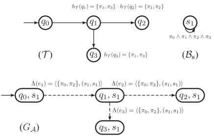
Figure 7: Example 10. $\mathcal{T}$: part of the system; $\mathcal{B}_{\mathbf{s}}$: part of the specification automaton; $G_{\mathcal{A}}$: part of the graph that corresponds to the product automaton.

A valid relaxation $\mathcal{B}$ should produce a reachable $v_{f}\in V_{f}$ with prefix and lasso path such that $\mathcal{L}(\mathcal{T}\times\mathcal{B})\neq\emptyset$. The next section provides an algorithmic solution to this problem.

V A Heuristic Algorithm for MRP

In this section, we present an approximation algorithm (AAMRP) for the Minimal Revision Problem (MRP). It is based on Dijkstra’s shortest path algorithm (Cormen et al. 2001). The main difference from Dijkstra’s algorithm is that instead of finding the minimum weight path to reach each node, AAMRP tracks the number of atomic propositions that must be removed from each edge on the paths of the graph $G_{\mathcal{A}}$.

The pseudocode for the AAMRP is presented in Algorithms 1 and 2. The main algorithm (Alg. 1) divides the problem into two tasks. First, in Line 5, it finds an approximation to the minimum number of atomic propositions from $\overline{\Pi}$ that must be removed to have a prefix path to each reachable sink (see Section III-A). Then, in Line 8, it repeats the process from each reachable final state to find an approximation to the minimum number of atomic propositions that must be removed so that a lasso path is enabled. The combination of prefix/lasso that removes the minimal number of atomic propositions is returned to the user. We remark that from line 10, a set of atomic propositions found from prefix part is used when it starts searching for lasso path of every reachable $v_{f}\in\mathcal{V}\cap V_{f}$.

Inputs: a graph $G_{\mathcal{A}}=(V,E,v_{s},V_{f},\overline{\Pi},\Lambda)$.
Outputs: the list $L$ of atomic propositions form $\overline{\Pi}$ that must be removed $\mathcal{B}_{\mathbf{s}}$.

Algorithm 1 AAMRP

1:procedure AAMRP($G_{\mathcal{A}}$)

2:     $L\leftarrow\overline{\Pi}$

3:     $\mathcal{M}[:,:]\leftarrow(\overline{\Pi},\infty)$

4:     $\mathcal{M}[v_{s},:]\leftarrow(\emptyset,0)$ $\triangleright$ Initialize the source node

5:     $\left\langle\mathcal{M},\mathbf{P},\mathcal{V}\right\rangle\leftarrow\text{\sc FindMinPath}(G_{\mathcal{A}},\mathcal{M},0)$

6:     $\text{\sc Acceptable}\leftarrow False$

7:     for $v_{f}\in\mathcal{V}\cap V_{f}$ do

8:         $L_{p}\leftarrow\text{\sc GetAPFromPath}(v_{s},v_{f},\mathcal{M},\mathbf{P})$

9:         $\mathcal{M}^{\prime}[:,:]\leftarrow(\overline{\Pi},\infty)$

10:         $\mathcal{M}^{\prime}[v_{f},:]\leftarrow(L_{p},|L_{p}|)$ $\triangleright$ Store APs from prefix path $v_{s}\leadsto v_{f}$ to $\mathcal{M}^{\prime}[v_{f},:]$

11:         $G_{\mathcal{A}}^{\prime}\leftarrow(V,E,v_{f},\{v_{f}\},\overline{\Pi},\Lambda)$

12:         $\left\langle\mathcal{M}^{\prime},\mathbf{P}^{\prime},\mathcal{V}^{\prime}\right\rangle\leftarrow\text{\sc FindMinPath}(G^{\prime}_{\mathcal{A}},\mathcal{M}^{\prime},1)$

13:         if $v_{f}\in\mathcal{V}^{\prime}$ then

14:              $L^{\prime}\leftarrow\text{\sc GetAPFromPath}(v_{f},v_{f},\mathcal{M}^{\prime},\mathbf{P}^{\prime})$ $\triangleright$ Get APs of prefix $v_{s}\leadsto v_{f}$ and lasso $v_{f}\leadsto v_{f}$ from $\mathcal{M}^{\prime}[v_{f},:]$

15:              if $|L^{\prime}|$ $\leq|L|$ then

16:                  $L\leftarrow L^{\prime}$

17:              end if

18:              $\text{\sc Acceptable}\leftarrow True$

19:         end if

20:     end for

21:     if $\neg\text{\sc Acceptable}$ then

22:         $L\leftarrow\emptyset$

23:     end if

24:     return $L$

25:end procedure

The function GetAPFromPath($(v_{s},v_{f},\mathcal{M},\mathbf{P})$) returns the atomic propositions that must be removed from $\mathcal{B}_{\mathbf{s}}$ in order to enable a path on $\mathcal{A}$ from a starting state $v_{s}$ to a final state $v_{f}$ given the tables $\mathcal{M}$ and $\mathbf{P}$.

Algorithm 2 follows closely Dijkstra’s shortest path algorithm (Cormen et al. 2001). It maintains a list of visited nodes $\mathcal{V}$ and a table $\mathcal{M}$ indexed by the graph vertices which stores the set of atomic propositions that must be removed in order to reach a particular node on the graph. Given a node $v$, the size of the set $|\mathcal{M}[v,1]|$ is an upper bound on the minimum number of atomic propositions that must be removed. That is, if we remove all $\overline{\pi}\in\mathcal{M}[v,1]$ from $\mathcal{B}_{\mathbf{s}}$, then we enable a simple path (i.e., with no cycles) from a starting state to the state $v$. The size of $|\mathcal{M}[v,1]|$ is stored in $\mathcal{M}[v,2]$ which also indicates that the node $v$ is reachable when $\mathcal{M}[v,2]<\infty$.

The algorithm works by maintaining a queue with the unvisited nodes on the graph. Each node $v$ in the queue has as key the number of atomic propositions that must be removed so that $v$ becomes reachable on $\mathcal{A}$. The algorithm proceeds by choosing the node with the minimum number of atomic propositions discovered so far (line 18). Then, this node is used in order to updated the estimates for the minimum number of atomic propositions needed in order to reach its neighbors (line 22). A notable difference of Alg. 2 from Dijkstra’s shortest path algorithm is the check for lasso paths in lines 8-16. After the source node is used for updating the estimates of its neighbors, its own estimate for the minimum number of atomic propositions is updated either to the value indicated by the self loop or the maximum possible number of atomic propositions. This is required in order to compare the different paths that reach a node from itself.

Algorithm 2 FindMinPath

Inputs: a graph $G_{\mathcal{A}}=(V,E,v_{s},V_{f},\overline{\Pi},\Lambda)$, a table $\mathcal{M}$ and a flag $lasso$ on whether this is a lasso path search.
Variables: a queue $\mathcal{Q}$, a set $\mathcal{V}$ of visited nodes and a table $\mathbf{P}$ indicating the parent of each node on a path.
Output: the tables $\mathcal{M}$ and $\mathbf{P}$ and the visited nodes $\mathcal{V}$

1:procedure FindMinPath($G_{\mathcal{A}}$,$\mathcal{M}$,$lasso$)

2:     $\mathcal{V}\leftarrow\{v_{s}\}$

3:     $\mathbf{P}[:]\leftarrow\emptyset$ $\triangleright$ Each entry of $\mathbf{P}$ is set to $\emptyset$

4:     $\mathcal{Q}\leftarrow V-\{v_{s}\}$

5:     for $v\in V$ such that $(v_{s},v)\in E$ and $v\neq v_{s}$ do

6:         $\left\langle\mathcal{M},\mathbf{P}\right\rangle\leftarrow\text{\sc Relax}((v_{s},v),\mathcal{M},\mathbf{P},\Lambda)$

7:     end for

8:     if $lasso=1$ then

9:         if $(v_{s},v_{s})\in E$ then

10:              $\mathcal{M}[v_{s},1]\leftarrow\mathcal{M}[v_{s},1]\cup\Lambda(v_{s},v_{s})$

11:              $\mathcal{M}[v_{s},2]\leftarrow|\mathcal{M}[v_{s},1]\cup\Lambda(v_{s},v_{s})|$

12:              $\mathbf{P}[v_{s}]=v_{s}$

13:         else

14:              $\mathcal{M}[v_{s},:]\leftarrow(\overline{\Pi},\infty)$

15:         end if

16:     end if

17:     while $\mathcal{Q}\neq\emptyset$ do

18:         $u\leftarrow$ ExtractMIN($\mathcal{Q}$) $\triangleright$ Get node $u$ with minimum $\mathcal{M}[u,2]$

19:         if $\mathcal{M}[u,2]<\infty$ then

20:              $\mathcal{V}\leftarrow\mathcal{V}\cup\{u\}$

21:              for $v\in V$ such that $(u,v)\in E$ do

22:                  $\left\langle\mathcal{M},\mathbf{P}\right\rangle\leftarrow\text{\sc Relax}((u,v),\mathcal{M},\mathbf{P},\Lambda)$

23:              end for

24:         end if

25:     end while

26:     return $\mathcal{M}$, $\mathbf{P}$, $\mathcal{V}$

27:end procedure

Algorithm 3 Relax

Inputs: an edge $(u,v)$, the tables $\mathcal{M}$ and $\mathbf{P}$ and the edge labeling function $\Lambda$
Output: the tables $\mathcal{M}$ and $\mathbf{P}$

1:procedure Relax($(u,v)$,$\mathcal{M}$,$\mathbf{P}$,$\Lambda$)

2:     if $|\mathcal{M}[u,1]\cup\Lambda(u,v)|<\mathcal{M}[v,2]$ then

3:         $\mathcal{M}[v,1]\leftarrow\mathcal{M}[u,1]\cup\Lambda(u,v)$

4:         $\mathcal{M}[v,2]\leftarrow|\mathcal{M}[u,1]\cup\Lambda(u,v)|$

5:         $\mathbf{P}[v]\leftarrow u$

6:     end if

7:     return $\mathcal{M}$, $\mathbf{P}$

8:end procedure

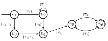
Figure 8: The graph of Example 11. The source $v_{s}=v_{1}$ is denoted by an arrow and the sink $v_{6}$ by double circle ($V_{f}=\{v_{6}\}$).

The following example demonstrates how the algorithm works and indicates the structural conditions on the graph that make the algorithm non-optimal.

Example 11.

Let us consider the graph in Fig. 8. The source node of this graph is $v_{s}=v_{1}$ and the set of sink nodes is $V_{f}=\{v_{6}\}$. The $\overline{\Pi}$ set of this graph is $\{\overline{\pi}_{1},\ldots,\overline{\pi}_{4}\}$. Consider the first call of FindMinPath (line 5 of Alg. 1).

• Before the first execution of the while loop (line 17): The queue contains $\mathcal{Q}=\{v_{2},\ldots,v_{6}\}$. The table $\mathcal{M}$ has the following entries: $\mathcal{M}{[v_{1},:]}=\left\langle\emptyset,0\right\rangle$, $\mathcal{M}{[v_{2},:]}=\left\langle\{\overline{\pi}_{1}\},1\right\rangle$, $\mathcal{M}{[v_{3},:]}=\left\langle\{\overline{\pi}_{1},\overline{\pi}_{3}\},2\right\rangle$, $\mathcal{M}{[v_{4},:]}=\ldots=\mathcal{M}{[v_{6},:]}=\left\langle\overline{\Pi},\infty\right\rangle$.

• Before the second execution of the while loop (line 17): The node $v_{2}$ was popped from the queue since it had $\mathcal{M}{[v_{2},2]}=1$. The queue now contains $\mathcal{Q}=\{v_{3},\ldots,v_{6}\}$. The table $\mathcal{M}$ has the following rows: $\mathcal{M}{[v_{1},:]}=\left\langle\emptyset,1\right\rangle$, $\mathcal{M}{[v_{2},:]}=\left\langle\{\overline{\pi}_{1}\},1\right\rangle$, $\mathcal{M}{[v_{3},:]}=\left\langle\{\overline{\pi}_{1},\overline{\pi}_{3}\},2\right\rangle$, $\mathcal{M}{[v_{4}]}=\left\langle\{\overline{\pi}_{1},\overline{\pi}_{2}\},2\right\rangle$, $\mathcal{M}{[v_{5},:]}=\mathcal{M}{[v_{6},:]}=\left\langle\overline{\Pi},\infty\right\rangle$.

• At the end of FindMinPath (line 27): The queue now is empty. The table $\mathcal{M}$ has the following rows: $\mathcal{M}{[v_{1},:]}=\left\langle\emptyset,0\right\rangle$, $\mathcal{M}{[v_{2},:]}=\left\langle\{\overline{\pi}_{1}\},1\right\rangle$, $\mathcal{M}{[v_{3},:]}=\left\langle\{\overline{\pi}_{1},\overline{\pi}_{3}\},2\right\rangle$, $\mathcal{M}{[v_{4},:]}=\left\langle\{\overline{\pi}_{1},\overline{\pi}_{2}\},2\right\rangle$, $\mathcal{M}{[v_{5},:]}=\left\langle\{\overline{\pi}_{1},\overline{\pi}_{2},\overline{\pi}_{4}\},3\right\rangle$, $\mathcal{M}{[v_{6},:]}=\left\langle\overline{\Pi},4\right\rangle$, which corresponds to the path $v_{1}$, $v_{2}$, $v_{4}$, $v_{5}$, $v_{6}$.

Note that algorithm returns a set of atomic propositions $L^{\prime}=\overline{\Pi}$ which is not optimal $|L^{\prime}|$ $=4$. The path $v_{1}$, $v_{3}$, $v_{4}$, $v_{5}$, $v_{6}$ would return $L^{\prime}$ $=\{\overline{\pi}_{1},\overline{\pi}_{3},\overline{\pi}_{4}\}$ with $|L^{\prime}|$ $=3$. $\bigtriangleup$

Correctness: The correctness of the algorithm AAMRP is based upon the fact that a node $v\in V$ is reachable on $G_{\mathcal{A}}$ if and only if $\mathcal{M}[v,2]<\infty$. The argument for this claim is similar to the proof of correctness of Dijkstra’s shortest path algorithm in Cormen et al. 2001. If this algorithm returns a set of atomic propositions $L$ which removed from $\mathcal{B}_{\mathbf{s}}$, then the language $\mathcal{L}(\mathcal{A})$ is non-empty. This is immediate by the construction of the graph $G_{\mathcal{A}}$ (Def. 7).

We remark that AAMRP does not solve Problem 2 exactly since MRP is NP-Complete. However, AAMRP guarantees that it returns a valid relaxation $\mathcal{B}$ where $\mathcal{B}_{\mathbf{s}}\preceq\mathcal{B}$.

Theorem 1.

If a valid relaxation exists, then AAMRP always returns a valid relaxation $\mathcal{B}$ of some initial $\mathcal{B}_{\mathbf{s}}$ such that $\mathcal{L}(\mathcal{T}\times\mathcal{B})\neq\emptyset$.

Proof.

First, we will show that if AAMRP returns $\emptyset$, then there is no valid relaxation of $\mathcal{B}_{\mathbf{s}}$. AAMRP returns $\emptyset$ when there is no reachable $v_{f}\in V_{f}$ with prefix and lasso path or GetAPFromPath returns $\emptyset$. If there is no reachable $v_{f}$, then either the accepting state is not reachable on $\mathcal{B}_{\mathbf{s}}$ or on $\mathcal{T}$. Recall that the Def. 7 constructs a graph where all the transitions of $\mathcal{T}$ and $\mathcal{B}$ are possible. If it returns $\emptyset$ as a valid solution, then there is a path on the graph that does not utilize any labeled edge by $\Lambda$. Thus, $\mathcal{L}(\mathcal{T}\times\mathcal{B}_{\mathbf{s}})\neq\emptyset$. Since we assume that $\mathcal{B}_{\mathbf{s}}$ is unsatisfiable on $\mathcal{T}$, this is contradiction.

Second, without loss of generality, suppose that AAMRP returns $\widetilde{\Lambda}(\mu)$. Using this $\widetilde{\Lambda}(\mu)$, we can build a relax specification automaton $\mathcal{B}$. Using each $\left\langle l,(s,s^{\prime}),k\right\rangle\in\widetilde{\Lambda}(\mu)$ and for each $\pi\in l$, we add the indices of the literal $\phi_{ij}$ in $\Phi_{\mathcal{B}_{\mathbf{s}}(s,s^{\prime})}$ that corresponds to $\pi$ to the sets $\hat{D}_{ss^{\prime}}$ and $\hat{C}^{i}_{ss^{\prime}}$. The resulting substitution $\theta$ produces a relaxation. Moreover, it is a valid relaxation, because by removing the atomic propositions in $\theta$ from $\mathcal{B}_{\mathbf{s}}$, we get a path that satisfies the prefix and lasso components on the product automaton. ∎

Running time: The running time analysis of the AAMRP is similar to that of Dijkstra’s shortest path algorithm. In the following, we will abuse notation when we use the $O$ notation and treat each set symbol $S$ as its cardinality $|S|$.

First, we will consider FindMinPath. The fundamental difference of AAMRP over Dijkstra’s algorithm is that we have set theoretic operations. We will assume that we are using a data structure for sets that supports $O(1)$ set cardinality quarries, $O(\log n)$ membership quarries and element insertions (Cormen et al. 2001) and $O(n)$ set up time. Under the assumption that $\mathcal{Q}$ is implemented in such a data structure, each ExtractMIN takes $O(\log V)$ time. Furthermore, we have $O(V)$ such operations (actually $|V|-1$) for a total of $O(V\log V)$.

Setting up the data structure for $\mathcal{Q}$ will take $O(V)$ time. Furthermore, in the worst case, we have a set $\Lambda(e)$ for each edge $e\in E$ with set-up time $O(E\overline{\Pi})$. Note that the initialization of $\mathcal{M}[v,:]$ to $\left\langle\overline{\Pi},\infty\right\rangle$ does not have to be implemented since we can have indicator variables indicating when a set is supposed to contain all the (known in advance) elements.

Assuming that $E$ is stored in an adjacency list, the total number of calls to Relax at lines 5 and 21 of Alg. 2 will be $O(E)$ times. Each call to Relax will have to perform a union of two sets ($\mathcal{M}[u,1]$ and $\Lambda(u,v)$). Assuming that both sets have in the worst case $|\overline{\Pi}|$ elements, each union will take $O(\overline{\Pi}\log\overline{\Pi})$ time. Finally, each set size quarry takes $O(1)$ time and updating the keys in $\mathcal{Q}$ takes $O(\log V)$ time. Therefore, the running time of FindMinPath is $O(V+E\overline{\Pi}+V\log V+E(\overline{\Pi}\log\overline{\Pi}+\log V))$.

Note that even if under Assumption 1 all nodes of $\mathcal{T}$ are reachable $(|V|<|E|)$, the same property does not hold for the product automaton. (e.g, think of an environment $\mathcal{T}$ and a specification automaton whose graphs are Directed Acyclic Graphs (DAG). However, even in this case, we have $(|V|<|E|)$. The running time of FindMinPath is $O(E(\overline{\Pi}\log\overline{\Pi}+\log V))$. Therefore, we observe that the running time also depends on the size of the set $\overline{\Pi}$. However, such a bound is very pessimistic since not all the edges will be disabled on $\mathcal{A}$ and, moreover, most edges will not have the whole set $\overline{\Pi}$ as candidates for removal.

Finally, we consider AAMRP. The loop at line 7 is going to be called $O(V_{f})$ times. At each iteration, FindMinPath is called. Furthermore, each call to GetAPFromPath is going to take $O(V\overline{\Pi}\log\overline{\Pi})$ time (in the worst case we are going to have $|V|$ unions of sets of atomic propositions). Therefore, the running time of AAMRP is $O(V_{f}(V\overline{\Pi}\log\overline{\Pi}+E(\overline{\Pi}\log\overline{\Pi}+\log V)))=O(V_{f}E(\overline{\Pi}\log\overline{\Pi}+\log V))$ which is polynomial in the size of the input graph.

Approximation bound: AAMRP does not have a constant approximation ratio on arbitrary graphs.

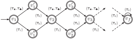
Figure 9: The graph of Example 12. The source $v_{s}=v_{1}$ is denoted by an arrow and the sink $v_{f}$ by double circle ($V_{f}=\{v_{f}\}$).

Example 12 (Unbounded Approximation).

The graph in Fig. 9 is the product of a specification automaton with a single state and a self transition with label $\{\overline{\pi}_{0},\overline{\pi}_{1},\ldots,\overline{\pi}_{m},\overline{\pi}_{\bigstar},\overline{\pi}_{\clubsuit}\}$ and an environment automaton with the same structure as the graph in Fig. 9 but with appropriately defined state labels. In this graph, AAMRP will choose the path $v_{1}$,$v_{1}^{\prime\prime}$, $v_{2}$, $v_{2}^{\prime\prime}$, $v_{3}$, $\ldots$, $v_{f}$. The corresponding revision will be the set of atomic propositions $L_{p}=\{\overline{\pi}_{0},\overline{\pi}_{1},\overline{\pi}_{2},\ldots,\overline{\pi}_{m}\}$ with $|L_{p}|=m+1$. This is because in $v_{2}$, AAMRP will choose the path through $v_{1}^{\prime\prime}$ rather than $v_{1}^{\prime}$ since the latter will produce a revision set of size $|\{\overline{\pi}_{0},\overline{\pi}_{\bigstar},\overline{\pi}_{\clubsuit}\}|=3$ while the former a revision set of size $|\{\overline{\pi}_{0},\overline{\pi}_{1}\}|=2$. Similarly at the next junction node $v_{3}$, the two candidate revision sets $\{\overline{\pi}_{0},\overline{\pi}_{1},\overline{\pi}_{\bigstar},\overline{\pi}_{\clubsuit}\}$ and $\{\overline{\pi}_{0},\overline{\pi}_{1},\overline{\pi}_{2}\}$ have sizes 4 and 3, respectively. Therefore, the algorithm will always choose the path through the nodes $v_{i}^{\prime\prime}$ rather than $v_{i}^{\prime}$ producing, thus, a solution of size $m+1$. However, in this graph, the optimal revision would have been $L_{p}=\{\overline{\pi}_{0},\overline{\pi}_{\bigstar},\overline{\pi}_{\clubsuit}\}$ with $|L_{p}|=3$. Hence, we can see that in this example for $m>2$ AAMRP returns a solution which is $m-2$ times bigger than the optimal solution. $\bigtriangleup$

There is also a special case where AAMRP returns a solution whose size is at most twice the size of the optimal solution.

Theorem 2.

AAMRP on planar Directed Acyclic Graphs (DAG) where all the paths merge on the same node is a 2-approximation algorithm.

The proof is provided in the Appendix X.

VI Examples and Numerical Experiments

In this section, we present experimental results using our prototype implementation of AAMRP. The prototype implementation is in Python (see Kim 2014b). Therefore, we expect the running times to substantially improve with a C implementation using state-of-the-art data structure implementations.

We first present some examples and expand few more example scenarios.

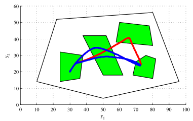
Figure 10: The simple environment of Example 13 along with a low speed mobile robot trajectory that satisfies the specification.

Example 13.

We revisit Example 1. The product automaton of this example has 85 states, 910 transitions and 17 reachable final states. It takes 0.095 sec by AAMRP. AAMRP returns the set of atomic propositions $\{\left\langle\pi_{4},(s_{2},s_{4})\right\rangle\}$ as a minimal revision to the problem, which is revision (3) among the three minimal revisions of the example: one of the blue trajectories in Fig. 10. Thus, it is an optimal solution. $\bigtriangleup$

Example 14.

We revisit Example 2. The graph of this example has 36 states, 240 transitions and 9 reachable sinks. AAMRP returns the set of atomic propositions $\{\left\langle\pi_{13},(s_{2},s_{3})\right\rangle\}$ as minimal revision to the problem. It takes 0.038 sec by AAMRP. Intuitively, AAMRP recommends dropping the requirement that $\pi_{13}$ should be reached from the specification. Therefore, Object 1 will remain where it is, while Object 2 will follow the path $q_{1}$, $q_{2}$, $q_{3}$, $q_{2}$, $q_{3}$, …. $\bigtriangleup$

With our prototype implementation, we could expand our experiment to few more example scenarios introduced in Ulusoy et al. 2011, 2012.

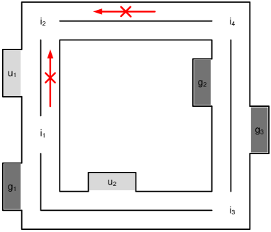
Figure 11: Schematic illustration of the simple road network environment of Example 15. The robot is required to drive right-side of the road.

Example 15 (Single Robot Data Gathering Task).

In this example, we use a simplified road network having three gathering locations and two upload locations with four intersections of the road. In Fig. 11, the data gather locations, which are labeled $g_{1}$, $g_{2}$, and $g_{3}$, are dark gray, the data upload locations, which are labeled $u_{1}$ and $u_{2}$, are light gray, and the intersections are labeled $i_{1}$ through $i_{4}$. In order to gather data and upload the gather-data persistently, the following LTL formula may be considered: $\phi_{A}$ $:=$ GF($\varphi_{g}$) $\wedge$ GF($\pi$), where $\varphi_{g}:=g_{1}\vee g_{2}\vee g_{3}$ and $\pi:=u_{1}\vee u_{2}$. The following formula can make the robot move from gather locations to upload locations after gathering data: $\phi_{G}$ $:=$ G($\varphi_{g}\rightarrow$ X($\neg\varphi_{g}\,\mathcal{U}\pi$). In order for the robot to move to gather location after uploading, the following formula is needed: $\phi_{U}$ $:=$ G($\pi\rightarrow$ X($\neg\pi\,\mathcal{U}\varphi_{g}$).

Let us consider that some parts of road are not recommended to drive from gather locations, such as from $i_{4}$ to $i_{2}$ and from $i_{1}$ to $i_{2}$. We can describe those constraints as following: $\psi_{1}$ $:=$ G($g_{1}$ $\rightarrow$ $\neg$($i_{4}$ $\wedge$ X$i_{2}$)$\,\mathcal{U}$$u_{1}$) and $\psi_{2}$ $:=$ G($g_{2}$ $\rightarrow$ $\neg$($i_{1}$ $\wedge$ X$i_{2}$)$\,\mathcal{U}$$u_{2}$). If the gathering task should have an order such as $g_{3}$, $g_{1}$, $g_{2}$, $g_{3}$, $g_{1}$, $g_{2}$, $\ldots$, then the following formula could be considered: $\phi_{O}$ := (($\neg$$g_{1}$ $\wedge$ $\neg$$g_{2}$)$\,\mathcal{U}$$g_{3}$) $\wedge$ G($g_{3}$ $\rightarrow$ X(($\neg$$g_{2}$ $\wedge$ $\neg$$g_{3}$)$\,\mathcal{U}$$g_{1}$)) $\wedge$ G($g_{1}$ $\rightarrow$ X(($\neg$$g_{1}$ $\wedge$ $\neg$$g_{3}$)$\,\mathcal{U}$$g_{2}$)) $\wedge$ G($g_{2}$ $\rightarrow$ X(($\neg$$g_{1}$ $\wedge$ $\neg$$g_{2}$)$\,\mathcal{U}$$g_{3}$)). Now, we can informally describe the mission. The mission is “Always gather data from g3, g1, g2 in this order and upload the collected data to $u_{1}$ and $u_{2}$. Once data gathering is finished, do not visit gather locations until the data is uploaded. Once uploading is finished, do not visit upload locations until gathering data. You should always avoid the road from $i_{4}$ to $i_{2}$ when you head to $u_{1}$ from $g_{1}$ and the road from $i_{1}$ to $i_{2}$ when you head to $u_{2}$ from $g_{2}$”. The following formula represents this mission:

$\phi_{single}$ := $\phi_{O}\wedge\phi_{G}\wedge\phi_{U}\wedge\psi_{1}\wedge\psi_{2}\wedge$ GF($\pi$).

Assume that initially, the robot is in $i_{3}$ and all nodes are final nodes. When we made a cross product with the road and the specification, we could get 36824 states, 350114 edges, and 450 final states. Not removing some atomic propositions, the specification was not satisfiable. AAMRP took 15 min 34.572 seconds, and suggested removing $g_{3}$. Since the original specification has many $g_{3}$ in it, we had to trace which $g_{3}$ from the specification should be removed. Hence, we revised the LTL2BA (Gastin and Oddoux (2001)), indexing each atomic proposition on the transitions and states (see Kim 2014a).Two $g_{3}$ are mappped to the same transition on the specification automaton in ($\neg$$g_{1}$ $\wedge$ $\neg$$g_{2}$)$\,\mathcal{U}$$g_{3}$ of $\phi_{O}$ and in $\varphi_{g}:=g_{1}\vee g_{2}\vee g_{3}$ in $\phi_{U}$. $\bigtriangleup$

The last example shows somewhat different missions with multiple robots. If the robots execute the gather and upload mission, persistently, we could assume that the battery in the robots should be recharged.

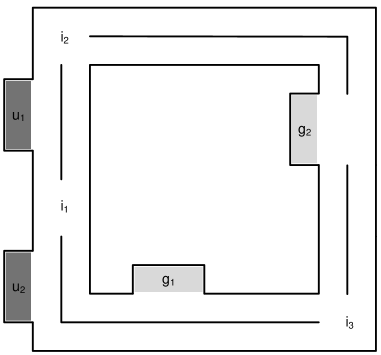
Figure 12: Schematic illustration of the simple road network environment of Example 16. The robots can stay upload locations $u_{1}$ and $u_{2}$ to recharge the battery.

Example 16 (Charging while Uploading).

In this exaple, we assume that robots can recharge their battery in upload locations so that robots are reqired to stay at the upload locations as much as possible. We also assume that each gathering localtion has a dedicated upload location such that $g_{1}$ has $u_{1}$ as an upload location, and $g_{2}$ has $u_{2}$ as an upload location. For this example, we revised the road network so that we remove the gather location $g_{3}$ and the intersection $i_{4}$ to make the network simpler for this mission. We also positioned the upload locations next to each other. We assume that the power source is shared and it has just two charging statations (see in Fig. 12). We can describe the mission as follows: “Once $robot_{1}$ finishes gathering data at $g_{1}$, $robot_{1}$ should not visit the gather locations until the data is uploaded at $u_{1}$. Once $robot_{2}$ fisniehs gathering data at $g_{2}$, $robot_{2}$ shoud not visit the gather locations until the data is uploaded at $u_{2}$. Once the data is uploaded at $u_{1}$ or $u_{2}$, $robot_{1}$ or $robot_{2}$ should stay there until a gather locaiton is not occupied. Persistently, gather data from $g_{1}$ and $g_{2}$, avoiding the road from $g_{2}$ to $i_{2}$.” The following formula represents this mission:

$\phi_{charging}$ := G($g_{11}$ $\rightarrow$ X($\neg$$g_{11}$ $\wedge$ $\neg$$g_{21}$) $\,\mathcal{U}$$u_{11}$) $\wedge$

G($g_{22}$ $\rightarrow$ X($\neg$$g_{22}$ $\wedge$ $\neg$$g_{12}$) $\,\mathcal{U}$$u_{22}$) $\wedge$

G($u_{11}$ $\rightarrow$ $u_{11}$ $\,\mathcal{U}$ $\neg$$g_{22}$) $\wedge$

G($u_{22}$ $\rightarrow$ $u_{22}$ $\,\mathcal{U}$ $\neg$$g_{11}$) $\wedge$

GF$g_{11}$ $\wedge$ GF$g_{22}$ $\wedge$

G$\neg$($g_{21}$ $\wedge$ X$i_{21}$) $\wedge$

G$\neg$($g_{22}$ $\wedge$ X$i_{22}$).

Assume that initially, $robot_{1}$ is in $i_{1}$, $robot_{2}$ is in $i_{2}$, and all nodes are final nodes. From the cross product with the road and the specification, there was 65966 states, 253882 transitions, and 504 final nodes. For this example, we computed a synchronized environtment for two robots, and in this environment, atomic propositions were duplicationed for each robot. For example, a gather location $g_{1}$ is duplicated to $g_{11}$ for $robot_{1}$ and $g_{12}$ for $robot_{2}$. With this synchronized environment, we could avoid robots to be colliding and to be in the same location at the same time. However, not removing some atomic propositions, the specification was unsatisfiable. AAMRP took 24 min 22.578 seconds, and suggested removing $u_{22}$ from $robot_{2}$. The two occurances of $u_{22}$ were in G($g_{22}$ $\rightarrow$ X($\neg$$g_{22}$ $\wedge$ $\neg$$g_{12}$) $\,\mathcal{U}$$u_{22}$) and in the second $u_{22}$ of G($u_{22}$ $\rightarrow$ $u_{22}$ $\,\mathcal{U}$ $\neg$$g_{11}$) as indicated by our modified LTL2BA toolbox. The suggested path from AAMRP for each robot is as followings:

$path_{robot_{1}}$ = $i_{11}$$i_{21}$$u_{11}$$u_{11}$$i_{11}$($i_{21}$$g_{21}$$i_{31}$$g_{11}$$i_{11}$$i_{21}$$u_{11}$$u_{11}$$u_{11}$$u_{11}$$u_{11}$$u_{11}$$u_{11}$$u_{11}$$u_{11}$$i_{11}$)⁺

$path_{robot_{2}}$ = $i_{22}$$u_{12}$$i_{12}$$u_{22}$$u_{22}$($u_{22}$$u_{22}$$u_{22}$$u_{22}$$u_{22}$$u_{22}$$u_{22}$$i_{32}$$g_{12}$$i_{12}$$i_{22}$$g_{22}$$i_{32}$$g_{12}$$i_{12}$$u_{22}$)⁺

$\bigtriangleup$

For the experiments, we utilized the ASU super computing center which consists of clusters of Dual 4-core processors, 16 GB Intel(R) Xeon(R) CPU X5355 @2.66 Ghz. Our implementation does not utilize the parallel architecture. The clusters were used to run the many different test cases in parallel on a single core. The operating system is CentOS release 5.5.

In order to assess the experimental approximation ratio of AAMRP, we compared the solutions returned by AAMRP with the brute-force search. The brute-force search is guaranteed to return a minimal solution to the MRP problem.

Nodes	BRUTE-FORCE SEARCH							AAMRP							RATIO
	TIMES (SEC)			SOLUTIONS (SIZE)				TIMES (SEC)			SOLUTIONS (SIZE)
	min	avg	max	min	avg	max	succ	min	avg	max	min	avg	max	succ	min	avg	max
9	0.037	0.104	1.91	1	1.97	5	200/200	0.022	0.061	1.17	1	1.975	5	200/200	1	1.0016	1.333
100	0.069	510.18	20786	1	3.277	13	198/200	0.038	0.076	0.179	1	3.395	15	200/200	1	1.0006	1.125
196	0.066	1025.44	25271	1	3.076	8	171/200	0.007	0.188	0.333	1	4.285	17	200/200	1	1	1
324	0.103	992.68	25437	1	2.379	6	158/200	0.129	0.669	1.591	1	4.155	20	200/200	1	1	1.2
400	0.087	1110.05	17685	1	2.692	6	143/200	0.15	0.669	1.591	1	5	24	200/200	1	1	1
529	0.14	2153.90	26895	1	2.591	5	137/200	0.382	1.88	4.705	1	5.115	30	200/200	1	1	1

TABLE I: Numerical Experiments: Number of nodes versus the results of brute-force search and AAMRP. Under the brute-force search and AAMRP columns the numbers indicate computation times in $\sec$. RATIO indicates the experimentally observed approximation ratio to the optimal solution.

Nodes	AAMRP
	TIMES
	min	avg	max	succ
1024	0.125	0.23	0.325	9/10
10000	15.723	76.164	128.471	9/10
20164	50.325	570.737	1009.675	8/10
50176	425.362	1993.449	4013.717	3/10
60025	6734.133	6917.094	7100.055	2/10

TABLE II: Numerical Experiments: Number of nodes versus the results of AAMRP. Under the TIMES columns the numbers indicate computation times in $\sec$.

We performed a large number of experimental comparisons on random benchmark instances of various sizes. We used the same instances which were presented in Kim et al. 2012; Kim and Fainekos 2012. The first experiment involved randomly generated DAGs. Each test case consisted of two randomly generated DAGs which represented an environment and a specification. Both graphs have self-loops on their leaves so that a feasible lasso path can be found. The number of atomic propositions in each instance was equal to four times the number of nodes in each acyclic graph. For example, in the benchmark where the graph had 9 nodes, each DAG had 3 nodes, and the number of atomic propositions was 12. The final nodes are chosen randomly and they represent 5%-40% of the nodes. The number of edges in most instances were 2-3 times more than the number of nodes.

Table I compares the results of the brute-force search with the results of AAMRP on test cases of different sizes (total number of nodes). For each graph size, we performed 200 tests and we report minimum, average and maximum computation times in second and minimum, average and maximum numbers of atomic propositions for each instance solution. AAMRP was able to finish the computation and returned a minimal revision for all the test cases, but brute-force search was not able to finish all the computation within a 8 hours window.

Our brute-force search checks all the combinations of atomic propositions. For example, given $n$ atomic propositions, it checks at most $2^{n}$ cases. It uses breath first search to check the reachability for the prefix and the lasso part. If it is reachable with the chosen atomic propositions, then it is finished. If it is not reachable, then it chooses another combination until it is reachable. Since brute-force search checks all the combinations of atomic propositions, the success mostly depends on the time limit of the test. We remark that the brute-force search was not able to provide an answer to all the test cases within a 8 hours window. The comparison for the approximation ratio was possible only for the test cases where brute-force search successfully completed the computation. Note that in the case of 529 Nodes, even though the maximum RATIO is 1, the maximum solution from brute-force does not match with the maximum solution from AAMRP. One is 5 and another is 30. This is because the number of success from brute-force search is 137 / 200 and only comparing this success with the ones from AAMRP, the maximum RATIO is still 1.

An interesting observation is that the maximum approximation ratio is experimentally determined to be less than 2. For the randomly generated graphs that we have constructed the bound apppears to be 1.333. However, as we showed in the example 12, it is not easy to construct random examples that produce higher approximation ratios. Such example scenarios must be carefully constructed in advance.

In the second numerical experiment, we attempted to determine the problem sizes that our prototype implementation of AAMRP in Python can handle. The results are presented in Table II. We observe that approximately 60,025 nodes would be the limit of the AAMRP implementation in Python.

VII Related work

The automatic specification revision problem for automata based planning techniques is a relatively new problem.

A related research problem is query checking Chechik and Gurfinkel 2003, Gurfinkel et al. 2002. In query checking, given a model of the system and a temporal logic formula $\phi$, some subformulas in $\phi$ are replaced with placeholders. Then, the problem is to determine a set of Boolean formulas such that if these formulas are placed into the placeholders. Then, the problem is to determine a set of Boolean formulas such that if these formulas are placed into the placeholders, then $\phi$ holds on the model. The problem of revision as defined here is substantially different from query checking. For one, the user does not know where to position the placeholders in the formula when the planning fails.

The papers Ding and Zhang 2005, Finger and Wassermann 2008 present an also related problem. It is the problem of revising a system model such that it satisfies a temporal logic specification. Along the same lines, one can study the problem of maximally permissive controllers for automata specification Thistle and Wonham 1994. Note that in this paper, we are trying to solve the opposite problem, i.e., we are trying to relax the specification such that it can be realized on the system. The main motivation for our work is that the model of the system, i.e., the environment and the system dynamics, cannot be modified and, therefore, we need to understand what we can be achieved with the current constraints.

Finding out why a specification is not satisfiable on a model is a problem that is very related to the problems of vacuity and coverage in model checking Kupferman et al. 2008. Another related problem is the detection of the causes of unrealizability in LTL games. In this case, a number of heuristics have been developed in order to localize the error and provide meaningful information to the user for debugging Cimatti et al. 2008; Konighofer et al. 2009. Along these lines, LTLMop Raman and Kress-Gazit 2011 was developed to debug unrealizable LTL specifications in reactive planning for robotic applications. Raman et al. 2013 also provided an integrated system for non-expert users to control robots for high-level, reactive tasks through natural language. This system gives the user natural language feedback when the original intention is unsatisfiable. Raman and Kress-Gazit 2013 introduced an approach to analyze unrealizable robot specifications due to environment’s limitation. They provide how to find the minimal unsatisfiable cores, such as deadlock and livelock, for propositional encodings, searching for some sequence of states in the environment.

Over-Subscription Planning (OSP) Smith 2004 and Partial Satisfaction Planning (PSP) van den Briel et al. 2004 are also very related problems. OSP finds an appropriate subset of an over-subscribed, conjunctive goal to meet the limitation of time and energy consumption. PSP explains the planning problem where the goal is regarded as soft constraints and trying to find a good quality plan for a subset of the goals. OSP and PSP have almost same definition, but there is also a difference. OSP regards the resource limitations as an important factor of partial goal to be satisfied, while PSP chooses a trade-off between the total action costs and the goal utilities where handling the plan quality.

In Göbelbecker et al. 2010, the authors investigated situations in which a planner-based agent cannot find a solution for a given planning task. They provided a formalization of coming up with excuses for not being able to find a plan and determined the computational complexity of finding excuses. On the practical side, they presented a method that is able to find good excuses on robotic application domains.

Another related problem is the Minimum Constraint Removal Problem (MCR) Hauser 2012. MCR concentrates on finding the least set of violating geometric constraints so that satisfaction in the specification can be achieved.

In Cizelj and Belta 2013, authors introduced a related problem which is of automatic formula revision for Probabilistic Computational Tree Logic (PCTL) with noisy sensor and actuator. Their proposed approach uses some specification update rules in order to revise the specification formula until the supervisor is satisfied. Tumova et al. 2013 is closely related with our work. It takes as input a transition system, and a set of sub-specifications in LTL with each reward, and constructs a strategy maximizing the total reward of satisfiable sub-specifications. If a whole sub-specification is not feasible, then it is discarded. In our case, we try to minimize revising the sub-specification if it is infeasible. In Kim and Fainekos 2014, we also expended our approach with quantitative preference. While revising the sub-specification, it has two approaches to get revision. Instead of finding minimum number of atomic propositions, it tries to minimize the sum of preference levels of the atomic propositions and to minimize the maximum preference level of the atomic propositions.

VIII Conclusions

In this paper, we proved that the minimal revision problem for specification automata is NP-complete. We also provided a polynomial time approximation algorithm for the problem of minimal revision of specification automata and established its upper bound for a special case. Furthermore, we provided examples to demonstrate that an approximation ratio cannot be established for this algorithm.

The minimal revision problem is useful when automata theoretic planning fails and the modification of the environment is not possible. In such cases, it is desirable that the user receives feedback from the system on what the system can actually achieve. The challenge in proposing a new specification automaton is that the new specification should be as close as possible to the initial intent of the user. Our proposed algorithm experimentally achieves approximation ratio very close to 1. Furthermore, the running time of our prototype implementation is reasonable enough to be able to handle realistic scenarios.

Future research will proceed along several directions. Since the initial specification is ultimately provided in some form of natural language, we would like the feedback that we provide to be in a natural language setting as well. Second, we plan on developing a robust and efficient publicly available implementation of our approximation algorithm.

IX Appendix: NP-completeness of the Minimal Connecting Edge Problem

We will prove the Minimal Connecting Edge (MCE) problem is NP-Complete. MCE is a slightly simpler version of the Minimal Accepting Path (MAP) problem and, thus, MAP is NP-Complete as well.

In MCE, we consider a directed graph $G=(E,V)$ with a source $s$ and a sink $t$ where there is no path from $s$ to $t$. We also have a set of candidate edges $\hat{E}$ to be added to $E$ such that the graph becomes connected and there is a path from $s$ to $t$. Note that if the edges in $\hat{E}$ have no dependencies between them, then there exists an algorithm that can solve the problem in polynomial time. For instance, Dijkstra’s algorithm Cormen et al. 2001 applied on the weighted directed graph $G=(V,E\cup\hat{E},w)$ where the edges in $\hat{E}$ are assigned weight 1 and the edges in E are assigned weight $0$ solves the problem efficiently.

However, in MCE, the set $\hat{E}$ is partitioned in a number of classes $\hat{E}_{1},...,\hat{E}_{n}$ such that if an edge $e_{i}$ is added from $\hat{E}_{i}$, then all the other edges in $\hat{E}_{i}$ are added as well to $G$. This corresponds to the fact that if we remove a predicate from a transition in $\mathcal{B}_{\mathbf{s}}$, then a number of transitions on $G_{\mathcal{A}}$ are affected. Let us consider the $G_{\mathcal{A}}$ in Fig. 7 as an example. Here, $e_{0}$, $e_{2}$ and $e_{4}$ correspond to $y((s_{1},s_{1}),\pi_{0})$, $e_{1}$ and $e_{5}$ to $y((s_{1},s_{1}),\pi_{2})$ and $e_{3}$ to $y((s_{1},s_{1}),\pi_{3})$. Thus, $\{e_{0},e_{1},e_{2},e_{3},e_{4},e_{5}\}\in\hat{E}$ and there exist three classes $\hat{E}_{i}$, $\hat{E}_{j}$ and $\hat{E}_{j}$ in the partition such that $\{e_{0},e_{2},e_{4}\}\subseteq\hat{E}_{i}$, $\{e_{1},e_{5}\}\subseteq\hat{E}_{j}$ and $e_{3}\in\hat{E}_{k}$.

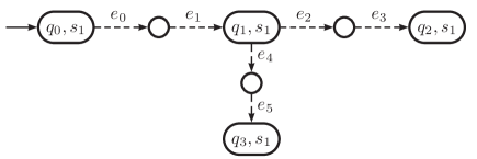
Figure 13: The MCE instance that corresponds to $G_{\mathcal{A}}$ from Fig. 7. The dashed edges denote candidate edges in $\hat{E}$.

Problem 3 (Minimal Connecting Edge (MCE)).

Input: Let $G=(V,E)$ be a directed graph with a source $s$ and a distinguished sink node $t$. We assume that there is no path in $G$ from $s$ to $t$. Let $\hat{E}\subseteq V\times V$ be a set such that $\hat{E}\cap E=\emptyset$. We partition $\hat{E}$ into $\mathcal{E}=\{\hat{E}_{1},\ldots,\hat{E}_{m}\}$. Each edge $e\in\hat{E}$ has a weight $W(e)\geq 0$.

Output: Given a weight limit $W$, determine if there is a selection of edges $R\subseteq\hat{E}$ such that

1. there is a path from $s$ to $t$ in the graph with all edges $E\cup R$,

2. $\sum_{e\in\cup\mathcal{R}}W(e)\leq W$ and

3. For each $\hat{E}_{i}\in\mathcal{E}$, if $\hat{E}_{i}\cap R\not=\emptyset$ then $\hat{E}_{i}\subseteq R$.

Theorem 3.

MCE is NP-complete.

Proof.

The problem is trivially in NP. Given a selection of edges from $\hat{E}$, we can indeed verify that the source and sinks are connected, the weight limit is respected and that the selection is made up of a union of sets from the partition.

We now claim that the problem is NP-Complete. We will reduce from 3-CNF-SAT. Consider an instance of 3-CNF-SAT with variables $X=\{x_{1},\ldots,x_{n}\}$ and clauses $C_{1},\ldots,C_{m}$. Each clause is a disjunction of three literals. We will construct graph $G$ and family of edges $\mathcal{E}$. The graph $G$ has edges $E$ made up of variable and clause “gadgets”.

Variable Gadgets

For each variable $x_{i}$, we create $6$ nodes $u_{i}$, $u_{i}^{t}$, $v_{i}^{t}$, $u_{i}^{f}$, $v_{i}^{f}$, and $v_{i}$. The gadget is shown in Fig. 14. The node $u_{i}$ is called the entrance to the gadget and $v_{i}$ is called the exit. The idea is that if the variable is assigned true, we will take the path

$$u_{i}\rightarrow u_{i}^{t}\rightarrow v_{i}^{t}\rightarrow v_{i}$$

to traverse through the gadget from its entrance to exit. The missing edge $u_{i}^{t}\rightarrow v_{i}^{t}$ will be supplied by one of the edge sets. If we assign the variable to false, we will instead traverse

$$u_{i}\rightarrow u_{i}^{f}\rightarrow v_{i}^{f}\rightarrow v_{i}$$

Variable gadgets are connected to each other in $G$ by adding edges from $v_{1}$ to $u_{2}$, $v_{2}$ to $u_{3}$ and so on until $v_{n-1}\rightarrow u_{n}$. The node $u_{1}$ is the source node.

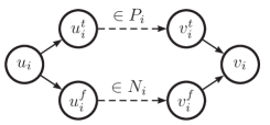
Figure 14: A single variable gadget. Solid edges are present in the original graph $G$ that will be constructed. Dashed edges $(u_{i}^{t},v_{i}^{t})$ or between $(u_{i}^{f},v_{i}^{f})$ will be supplied by one of the edge sets in $\hat{E}$.

Clause Gadgets

For each clause $C_{j}$ of the form $(\ell_{j1}\lor\ell_{j2}\lor\ell_{j3})$, we add a clause gadget consisting of eight nodes: entry node $a_{j}$, exit node $b_{j}$ and nodes $a_{j1},b_{j1}$, $a_{j2},b_{j2}$ and $a_{j3},b_{j3}$ corresponding to each of the three literals in the clause. The idea is that a path from the entry node $a_{j}$ to exit node $b_{j}$ will exist if the clause $C_{j}$ will be satisfied. Figure 15 shows how the nodes in a clause gadget are connected.

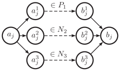
Figure 15: The clause gadget for a clause with three literals. The clause shown here is $(x_{1}\ \lor\ \overline{x_{2}}\ \lor\ \overline{x_{3}})$. The corresponding missing edges will be added to the set $P_{1},N_{2},N_{3}$, respectively, as shown in figure.

Structure

We connect $v_{n}$ the exit of the last variable gadget for variable $x_{n}$ to $a_{1}$, the entrance for first clause gadget. The sink node is $b_{m}$, the exit for the last clause gadget. Figure 16 shows the overall high level structure of the graph $G$ with variable and clause gadgets.

Figure 16: Connection between gadgets for variables and clauses.

Edge Sets

We design a family $\mathcal{E}=\{P_{1},\ldots,P_{n},N_{1},\ldots,N_{n}\}$. The set $P_{i}$ will correspond to a truth assignment of true to variable $x_{i}$ and $N_{i}$ correspond to a truth assignment of false to $x_{i}$.

$P_{i}$ has the edge $(u_{i}^{t},v_{i}^{t})$ of weight $1$ and for each clause $C_{j}$ containing the literal $x_{i}$, we add the missing edge $(a_{j}^{i},b_{j}^{i})$ corresponding to this literal in the clause gadget for $C_{j}$ to the set $P_{i}$ with weight $0$.

Similarly, $N_{i}$ has the edge from $(u_{i}^{f},v_{i}^{f})$ of weight $1$ and for each clause $C_{j}$ containing the literal $\overline{x_{i}}$ it has the missing edge in the clause gadget for $C_{j}$ with weight $0$. We ask if there is a way to connect the source $u_{1}$ with the sink $b_{m}$ with weight limit $\leq n$, where $n$ is the number of variables.

We verify that the sets $P_{1},\ldots,P_{n},N_{1},\ldots,N_{n}$ partition the set of missing edges.

Claim 1.

If there is a satisfying solution to the problem, then $u_{1}$ can be connected to $b_{m}$ by a choice of edge sets with total edge weight $\leq n$.

Proof.

Take a satisfying solution. If it assigns true to $x_{i}$, then choose all edges in $P_{i}$ else choose all edges $N_{i}$ if it assigns false. We claim that this will connect $u_{1}$ to $b_{m}$. First it is clear that since all variables are assigned, it will connect $u_{1}$ to $v_{n}$ by connecting one of the two missing links in each variable gadget. Corresponding to each clause, $C_{j}$ there will be a path from $a_{j}$ to $b_{j}$ in the clause gadget for $C_{j}$. This is because, at least one of the literals in the clause is satisfied and the corresponding set $P_{i}$ or $N_{i}$ will supply the missing edge. Furthermore, the weight of the selection will be precisely $n$, since we add exactly one edge in each variable gadget. ∎

Claim 2.

If there is a way to connect source to sink with weight $\leq n$ then a satisfying assignment exists.

Proof.

First of all, the total weight for any edge connection from source to sink is $\geq n$ since we need to connect $u_{1}$ to $v_{n}$ there are $n$ edges missing in any shortest path. The edges that will connect have weight $1$, each. Therefore, if there is a way to connect source to sink with weight $\leq n$, the total weight must in fact be $n$. This allows us to conclude that for every variable gadget precisely one of the missing edges is present. As a result, we can now form a truth assignment setting $x_{i}$ to true if $P_{i}$ is chosen and false if $N_{i}$ is. Therefore, the truth assignment will assign either true to $x_{i}$ or false and not both thanks to the weight limit of $n$. ∎

Next, we prove that each $a_{j}$ will be connected to $b_{j}$ in each clause gadget corr. to clause $C_{j}$. Let us assume that this was using the edge $(a_{j}^{i},b_{j}^{i})\in N_{i}$. Then, by construction have that $\overline{x_{i}}$ was in the clause $C_{j}$ which is now satisfied since $N_{i}$ is chosen, assigning $x_{i}$ to false. Similar reasoning can be used if $(a_{j},b_{j})\in P_{i}$. Combining, we conclude that all clauses are satisfied by our truth assignment. ∎

X Appendix: Upper Bound of the Approximation Ratio of AAMRP

We shall show the upper bound of the approximation algorithm (AAMRP) for a special case.

Theorem 4.

AAMRP on planar Directed Acyclic Graphs (DAG) where all the paths merge on the same node is a polynomial-time 2-approximation algorithm for the Minimal Revision Problem (MRP).

Proof.

We have already seen that the AAMRP runs in polynomial time.

Let $Y=\{y_{1},\ldots,y_{m}\}$ be a set of Boolean variables and $G:(V,E)$ be a graph with a labeling function $L:E\rightarrow\mathcal{P}(Y)$, wherein each edge $e\in E$ is labeled with a set of Boolean variables $L(e)\subseteq Y$. The label on an edge indicates that the edge is enabled iff all the Boolean variables on the edge are set to true. Let $v_{0}\in V$ be a marked initial state and $F\subseteq V$ be a set of marked final vertices.

Consider two functions $w^{\prime}:E^{*}\rightarrow\mathcal{P}(Y)$, and $w:E^{*}\rightarrow\mathbb{N}$ where $E^{*}$ represents the set of all finite sequences of edges of the graph $G$. Hence, $w^{\prime}(P)$ for a path $P=\langle v_{0},\ldots,v_{k}\rangle$ is a set of boolean variables of its constituent edges which makes them enabled on the path $P$:

$$w^{\prime}(P)=\bigcup\limits_{i=1}^{k}{L(v_{i-1},v_{i})}$$

while $w(P)$ is the number of the boolean variables of

$$w(P)=\Bigl{\lvert}\bigcup\limits_{i=1}^{k}{L(v_{i-1},v_{i})}\Bigr{\rvert}=\Bigl{\lvert}w^{\prime}(P)\Bigr{\rvert}$$

Given a initial vertex $v_{0}$, two vertices $v_{i}$, $v_{j}$, and a final vertex $v_{k}$, let $P_{opt}$ denote the path that produces an optimal revision for the given graph. Let $P_{a}$ denote a general revision by AAMRP. Suppose that $P_{opt}$ consists of subpaths $P_{0i}$, $P_{ij}$, $P_{jk}$, and $P_{a}$ consists of subpaths $P_{0i}$, $P^{\prime}_{ij}$, $P_{jk}$.

We will discuss the cases when $P_{0i}$ and $P_{jk}$ are empty later. The former case can occur when $P_{opt}$ and $P_{a}$ do not have any common edges from $v_{0}$ to $v_{i}$ in the sense that each path takes a different neighbor out of $v_{0}$. This case can also occur when $0<i$ if from $v_{0}$ to $v_{i}$ there is no boolean variables to be enabled to make the path activated. Likewise, the latter case can occur when $i<j<k$ or when $i\leq j=k$. We do not take $i=j$ unless $j=k$. Considering both cases together, we can get the possibility that $P_{opt}$ and $P_{a}$ are entirely different from $v_{0}$ to $v_{k}$.

In $v_{j}$, the AAMRP should relax the weight of the path from $v_{0}$ to $v_{j}$, comparing between two paths $P_{ij}$ and $P^{\prime}_{ij}$. Thus, we can denote:

$$w^{\prime}(P_{m})=w^{\prime}(P_{0i})\cup w^{\prime}(P^{\prime}_{ij})\cup w^{\prime}(P_{jk}),$$

$$w^{\prime}(P^{*})=w^{\prime}(P_{0i})\cup w^{\prime}(P_{ij})\cup w^{\prime}(P_{jk}).$$

Let $w^{\prime}(P_{0i})\cup w^{\prime}(P^{\prime}_{ij})=\Lambda_{a}$, $w^{\prime}(P_{0i})\cup w^{\prime}(P_{ij})=\Lambda_{opt}$, and $w^{\prime}(P_{jk})=\Lambda$. Then, we can denote:

$$w^{\prime}(P_{a})=\Lambda_{a}\cup\Lambda,$$

$$w^{\prime}(P_{opt})=\Lambda_{opt}\cup\Lambda.$$

Recall that

$$w(P_{a})=\lvert\Lambda_{a}\cup\Lambda\rvert,$$

$$w(P_{opt})=\lvert\Lambda_{opt}\cup\Lambda\rvert.$$

We will show that $w(P_{a})\leq 2w(P_{opt})$.

Note that $w(P_{opt})\geq 1$, so that $\lvert\Lambda_{opt}\cup\Lambda\rvert\geq 1$. This is because if $w(P_{opt})=0$, then it is reachable from $v_{0}$ to $v_{f}$ without enabling any boolean variables which are atomic propositions of the specification.

Remark 1.

$\lvert\Lambda_{opt}\cup\Lambda\rvert\geq 1$.

Note that $\lvert\Lambda_{a}\rvert\leq\lvert\Lambda_{opt}\rvert$. This is because the AAMRP only relaxes the path when it has less number of boolean variables.

Remark 2.

$\lvert\Lambda_{a}\rvert\leq\lvert\Lambda_{opt}\rvert$.

Note that if $\lvert\Lambda_{a}\rvert=0$, then $\lvert\Lambda_{opt}\cup\Lambda\rvert=\lvert\Lambda_{a}\cup\Lambda\rvert\leq 2\lvert\Lambda_{opt}\cup\Lambda\rvert$. In this case, $\Lambda_{a}$ is the optimal path if $\Lambda_{a}=0$ since $\Lambda$ is common for the two paths. I.e., $w(P_{a})\leq 2w(P_{opt})$.

Consider the case $\lvert\Lambda_{a}\rvert\geq 1$. We will prove the claim by contradiction. Assume that $2w(P_{opt})<w(P_{a})$ so that $2\lvert\Lambda_{opt}\cup\Lambda\rvert<\lvert\Lambda_{a}\cup\Lambda\rvert$. Let $\lvert\Lambda_{a}\rvert=\mu$, $\lvert\Lambda_{opt}\rvert=\eta$ and $\lvert\Lambda\rvert=\tau$. There are four cases.

Case 1: if $\Lambda_{opt}\cap\Lambda=\emptyset$ and $\Lambda_{a}\cap\Lambda=\emptyset$, then

$$2\lvert\Lambda_{opt}\cup\Lambda\rvert<\lvert\Lambda_{a}\cup\Lambda\rvert\Rightarrow 2(\eta+\tau)<\mu+\tau$$

$$2\eta+2\tau<\mu+\tau\Rightarrow 2\eta+\tau<\mu$$

However, $\mu\leq\eta$ by Remark 2. Thus, $\eta+\tau<0$ which is not possible and it contradicts our assumption.

Case 2: if $\Lambda_{opt}\cap\Lambda\neq\emptyset$ and $\Lambda_{a}\cap\Lambda=\emptyset$, then let $\lvert\Lambda_{opt}\cap\Lambda\rvert=\zeta$, where $1\leq\zeta\leq\min(\eta,\tau)$.

$$2\lvert\Lambda_{opt}\cup\Lambda\rvert<\lvert\Lambda_{a}\cup\Lambda\rvert\Rightarrow 2(\eta+\tau-\zeta)<\mu+\tau$$

$$2\eta+2\tau-2\zeta<\mu+\tau\Rightarrow 2\eta-2\zeta+\tau<\mu$$

If $\eta\leq\tau$, then $\zeta\leq\eta$ and $\eta=\zeta+\alpha$, for some $\alpha\geq 0$.

$$2(\zeta+\alpha)-2\zeta+\tau<\mu\Rightarrow 2\alpha+\tau<\mu$$

However, $\eta\leq\tau$ and $\mu\leq\eta$ by Remark 2. Thus, $2\alpha<0$ which is not possible and it contradicts our assumption.

If $\eta>\tau$ and $\eta=\tau+\beta$, for some $\beta>0$, then $\zeta\leq\tau$ and $\tau=\zeta+\alpha$, for some $\alpha\geq 0$.

$$2(\tau+\beta)-2\zeta+\tau<\mu\Rightarrow 2\tau-2\zeta+2\beta+\tau<\mu$$

$$2(\zeta+\alpha)-2\zeta+2\beta+\tau<\mu\Rightarrow 2\zeta+2\alpha-2\zeta+2\beta+\tau<\mu$$

$$2\alpha+2\beta+\tau<\mu\Rightarrow 2\alpha+2\beta+\eta-\beta<\mu$$

$$2\alpha+\beta+\eta<\mu$$

However, $\mu\leq\eta$ by Remark 2. Thus, $2\alpha+\beta<0$ which is not possible and it contradicts our assumption.

Case 3: if $\Lambda_{opt}\cap\Lambda=\emptyset$, $\Lambda_{a}\cap\Lambda\neq\emptyset$, then let $\lvert\Lambda_{a}\cap\Lambda\rvert=\theta$, where $1\leq\theta\leq\min(\mu,\tau)$.

$$2\lvert\Lambda_{opt}\cup\Lambda\rvert<\lvert\Lambda_{a}\cup\Lambda\rvert\Rightarrow 2(\eta+\tau)<\mu+\tau-\theta$$

$$2\eta+\tau<\mu-\theta\Rightarrow 2\eta+\tau<\mu$$

However, $\mu\leq\eta$ by Remark 2. Thus, $\eta+\tau<0$ which is not possible and it contradicts our assumption.

Finally the last case: if $\Lambda_{opt}\cap\Lambda\neq\emptyset$, $\Lambda_{a}\cap\Lambda\neq\emptyset$, then let $\lvert\Lambda_{opt}\cap\Lambda\rvert=\zeta$, where $1\leq\zeta\leq\min(\eta,\tau)$, and $\lvert\Lambda_{a}\cap\Lambda\rvert=\theta$, where $1\leq\theta\leq\min(\mu,\tau)$.

$$2\lvert\Lambda_{opt}\cup\Lambda\rvert<\lvert\Lambda\cup\Lambda\rvert\Rightarrow 2(\eta+\tau-\zeta)<\mu+\tau-\theta$$

$$2\eta+2\tau-2\zeta<\mu+\tau-\theta\Rightarrow 2\eta+\tau-2\zeta<\mu-\theta<\mu$$

If $\eta\leq\tau$, $\zeta\leq\eta$ and $\eta=\zeta+\alpha$, for some $\alpha\geq 0$, then

$$2(\zeta+\alpha)+\tau-2\zeta<\mu\Rightarrow 2\alpha+\tau<\mu$$

However, $\mu\leq\eta$ and $\eta\leq\tau$ by Remark 2. Thus, $2\alpha<0$ which is not possible and it contradicts our assumption.

If $\eta>\tau$, $\eta=\tau+\beta$, for some $\beta>0$, $\zeta\leq\tau$ and $\tau=\zeta+\alpha$, for some $\alpha\geq 0$, then

$$2\eta+\tau-2\zeta<\mu\Rightarrow\eta+(\tau+\beta)+\tau-2\zeta<\mu$$

$$\eta+(\zeta+\alpha)+\beta+(\zeta+\beta)-2\zeta<\mu\Rightarrow\eta+2\zeta+\alpha+2\beta-2\zeta<\mu$$

$$\eta+\alpha+2\beta<\mu$$

However, $\mu\leq\eta$ by Remark 2. Thus, $\alpha+2\beta<0$ which is not possible and it contradicts our assumption.

∎

Therefore, $\lvert\Lambda_{a}\cup\Lambda\rvert\leq 2\lvert\Lambda_{opt}\cup\Lambda\rvert$, and we can conclude that $w(P_{a})\leq 2w(P_{opt})$.

References

- Bhatia et al. [2010] A. Bhatia, L. E. Kavraki, and M. Y. Vardi. Sampling-based motion planning with temporal goals. In International Conference on Robotics and Automation, pages 2689–2696. IEEE, 2010.
- Bobadilla et al. [2011] Leonardo Bobadilla, Oscar Sanchez, Justin Czarnowski, Katrina Gossman, and Steven LaValle. Controlling wild bodies using linear temporal logic. In Proceedings of Robotics: Science and Systems, Los Angeles, CA, USA, June 2011.
- Buchi [1960] J. R. Buchi. Weak second order arithmetic and finite automata. Zeitschrift für Math. Logik und Grundlagen Math., 6:66–92, 1960.
- Chechik and Gurfinkel [2003] Marsha Chechik and Arie Gurfinkel. Tlqsolver: A temporal logic query checker. In Proceedings of the 15th International Conference on Computer Aided Verification, volume 2725, pages 210–214. Springer, 2003.
- Choset et al. [2005] Howie Choset, Kevin M. Lynch, Seth Hutchinson, George Kantor, Wolfram Burgard, Lydia E. Kavraki, and Sebastian Thrun. Principles of Robot Motion: Theory, Algorithms and Implementations. MIT Press, March 2005.
- Cimatti et al. [2008] A. Cimatti, M. Roveri, V. Schuppan, and A. Tchaltsev. Diagnostic information for realizability. In Francesco Logozzo, Doron Peled, and Lenore Zuck, editors, Verification, Model Checking, and Abstract Interpretation, volume 4905 of LNCS, pages 52–67. Springer, 2008.
- Cizelj and Belta [2013] Igor Cizelj and Calin Belta. Negotiating the probabilistic satisfaction of temporal logic motion specifications. In IEEE/RSJ International Conference on Intelligent Robots and Systems, 2013.
- Clarke et al. [1999] Edmund M. Clarke, Orna Grumberg, and Doron A. Peled. Model Checking. MIT Press, Cambridge, Massachusetts, 1999.
- Cormen et al. [2001] Thomas H. Cormen, Charles E. Leiserson, Ronald L. Rivest, and Cliff Stein. Introduction to Algorithms. MIT Press/McGraw-Hill, second edition, September 2001.
- Ding and Zhang [2005] Yulin Ding and Yan Zhang. A logic approach for ltl system modification. In 15th International Symposium on Foundations of Intelligent Systems, volume 3488 of LNCS, pages 435–444. Springer, 2005. ISBN 3-540-25878-7.
- Dzifcak et al. [2009] Juraj Dzifcak, Matthias Scheutz, Chitta Baral, and Paul Schermerhorn. What to do and how to do it: Translating natural language directives into temporal and dynamic logic representation for goal management and action execution. In Proceedings of the IEEE international conference on robotics and automation, 2009.
- Fainekos [2011] Georgios E. Fainekos. Revising temporal logic specifications for motion planning. In Proceedings of the IEEE Conference on Robotics and Automation, May 2011.
- Fainekos et al. [2009] Georgios E. Fainekos, Antoine Girard, Hadas Kress-Gazit, and George J. Pappas. Temporal logic motion planning for dynamic robots. Automatica, 45(2):343–352, February 2009.
- Filippidis et al. [2012] Ioannis Filippidis, Dimos V. Dimarogonas, and Kostas J. Kyriakopoulos. Decentralized multi-agent control from local LTL specifications. In 51st IEEE Conference on Decision and Control, pages pp. 6235–6240, 2012.
- Finger and Wassermann [2008] Marcelo Finger and Renata Wassermann. Revising specifications with CTL properties using bounded model checking. In Brazilian Symposium on Artificial Intelligence, volume 5249 of LNAI, page 157–166, 2008.
- Gastin and Oddoux [2001] P. Gastin and D. Oddoux. Fast LTL to Büchi automata translation. In G. Berry, H. Comon, and A. Finkel, editors, Proceedings of the 13th CAV, volume 2102 of LNCS, pages 53–65. Springer, 2001.
- Giacomo and Vardi [1999] Giuseppe De Giacomo and Moshe Y. Vardi. Automata-theoretic approach to planning for temporally extended goals. In European Conference on Planning, volume 1809 of LNCS, pages 226–238. Springer, 1999.
- Göbelbecker et al. [2010] Moritz Göbelbecker, Thomas Keller, Patrick Eyerich, Michael Brenner, and Bernhard Nebel. Coming up with good excuses: What to do when no plan can be found. In Proceedings of the 20th International Conference on Automated Planning and Scheduling (ICAPS). AAAI Press, may 2010.
- Gurfinkel et al. [2002] Arie Gurfinkel, Benet Devereux, and Marsha Chechik. Model exploration with temporal logic query checking. SIGSOFT Softw. Eng. Notes, 27(6):139–148, 2002.
- Hauser [2012] Kris Hauser. The minimum constraint removal problem with three robotics applications. In In Proceedings of the International Workshop on the Algorithmic Foundations of Robotics (WAFR), 2012.
- Karaman et al. [2008] S. Karaman, R. Sanfelice, and E. Frazzoli. Optimal control of mixed logical dynamical systems with linear temporal logic specifications. In IEEE Conf. on Decision and Control, 2008.
- Kim and Fainekos [2012] K. Kim and G. Fainekos. Approximate solutions for the minimal revision problem of specification automata. In Proceedings of the IEEE/RSJ International Conference on Intelligent Robots and Systems, 2012.
- Kim [2014a] Kangjin Kim. LTL2BA modification for indexing, 2014a. URL https://git.assembla.com/ltl2ba_cpslab.git.
- Kim [2014b] Kangjin Kim. Temporal logic specification revision and planning toolbox, 2014b. URL https://subversion.assembla.com/svn/temporal-logic-specification-revision-and-planning-toolbox/.
- Kim and Fainekos [2014] Kangjin Kim and Georgios Fainekos. Revision of specification automata under quantitative preferences. In Proceedings of the IEEE Conference on Robotics and Automation, 2014.
- Kim et al. [2012] Kangjin Kim, Georgios Fainekos, and Sriram Sankaranarayanan. On the revision problem of specification automata. In Proceedings of the IEEE Conference on Robotics and Automation, May 2012.
- Kloetzer and Belta [2010] M. Kloetzer and C. Belta. Automatic deployment of distributed teams of robots from temporal logic specifications. IEEE Transactions on Robotics, 26(1):48–61, 2010.
- Konighofer et al. [2009] R. Konighofer, G. Hofferek, and R. Bloem. Debugging formal specifications using simple counterstrategies. In Formal Methods in Computer-Aided Design, pages 152 –159. IEEE, November 2009.
- Kress-Gazit et al. [2008] Hadas Kress-Gazit, Georgios E. Fainekos, and George J. Pappas. Translating structured english to robot controllers. Advanced Robotics, 22(12):1343 –1359, 2008.
- Kress-Gazit et al. [2009] Hadas Kress-Gazit, Gerogios E. Fainekos, and George J. Pappas. Temporal logic based reactive mission and motion planning. IEEE Transactions on Robotics, 25(6):1370 – 1381, 2009.
- Kupferman et al. [2008] Orna Kupferman, Wenchao Li, and Sanjit A. Seshia. A theory of mutations with applications to vacuity, coverage, and fault tolerance. In Proceedings of the International Conference on Formal Methods in Computer-Aided Design, pages 25:1–25:9, Piscataway, NJ, USA, 2008. IEEE Press.
- Lacerda and Lima [2011] Bruno Lacerda and Pedro Lima. Designing petri net supervisors from ltl specifications. In Proceedings of Robotics: Science and Systems, Los Angeles, CA, USA, June 2011.
- LaValle [2006] Steven M. LaValle. Planning Algorithms. Cambridge University Press, 2006. URL http://msl.cs.uiuc.edu/planning/.
- LaViers et al. [2011] Amy LaViers, Magnus Egerstedt, Yushan Chen, and Calin Belta. Automatic generation of balletic motions. IEEE/ACM International Conference on Cyber-Physical Systems, 0:13–21, 2011.
- Park [1981] David Park. Concurrency and automata on infinite sequences. In Proceedings of the 5th GI-Conference on Theoretical Computer Science, pages 167–183. Springer-Verlag, 1981.
- Raman and Kress-Gazit [2011] Vasumathi Raman and Hadas Kress-Gazit. Analyzing unsynthesizable specifications for high-level robot behavior using LTLMoP. In 23rd International Conference on Computer Aided Verification, volume 6806 of LNCS, pages 663–668. Springer, 2011.
- Raman and Kress-Gazit [2013] Vasumathi Raman and Hadas Kress-Gazit. Towards minimal explanations of unsynthesizability for high-level robot behaviors. In 2013 IEEE/RSJ International Conference on Intelligent Robots and Systems, Tokyo, Japan, November 3-7, 2013, pages 757–762, 2013. doi: 10.1109/IROS.2013.6696436. URL http://dx.doi.org/10.1109/IROS.2013.6696436.
- Raman et al. [2013] Vasumathi Raman, Constantine Lignos, Cameron Finucane, Kenton C. T. Lee, Mitchell P. Marcus, and Hadas Kress-Gazit. Sorry dave, i’m afraid I can’t do that: Explaining unachievable robot tasks using natural language. In Robotics: Science and Systems IX, Technische Universität Berlin, Berlin, Germany, June 24 - June 28, 2013, 2013. URL http://www.roboticsproceedings.org/rss09/p23.html.
- Roy et al. [2011] Pritam Roy, Paulo Tabuada, and Rupak Majumdar. Pessoa 2.0: a controller synthesis tool for cyber-physical systems. In Proceedings of the 14th international conference on Hybrid systems: computation and control, HSCC ’11, pages 315–316, New York, NY, USA, 2011. ACM.
- Smith [2004] David E. Smith. Choosing objectives in over-subscription planning. In Proceedings of the 14th International Conference on Automated Planning and Scheduling (ICAPS-04), pages 393–401, 2004.
- Sniedovich [2006] Moshe Sniedovich. Dijkstra’s algorithm revisited: the dynamic programming connexion. Control and Cybernetics, 35(3):599–620, 2006.
- Thistle and Wonham [1994] J. G. Thistle and W. M. Wonham. Supervision of infinite behavior of discrete-event systems. SIAM J. Control Optim., 32(4):1098–1113, 1994. ISSN 0363-0129.
- Tumova et al. [2013] J. Tumova, L. I. Reyes Castro, S. Karaman, E. Frazzoli, and D. Rus. Minimum-violating planning with conflicting specifications. In American Control Conference, 2013.
- Ulusoy et al. [2011] Alphan Ulusoy, Stephen L. Smith, Xu Chu Ding, Calin Belta, and Daniela Rus. Optimal multi-robot path planning with temporal logic constraints. In IEEE/RSJ International Conference on Intelligent Robots and Systems,, pages 3087 –3092, 2011.
- Ulusoy et al. [2012] Alphan Ulusoy, Stephen L. Smith, Xu Chu Ding, and Calin Belta. Robust multi-robot optimal path planning with temporal logic constraints. In 2012 IEEE International Conference on Robotics and Automation (ICRA), 2012.
- van den Briel et al. [2004] Menkes van den Briel, Romeo Sanchez, Minh B. Do, and Subbarao Kambhampati. Effective approaches for partial satisfaction (over-subscription) planning. In Proceedings of the 19th national conference on Artifical intelligence, AAAI’04, pages 562–569. AAAI Press, 2004. ISBN 0-262-51183-5.
- Wongpiromsarn et al. [2010] Tichakorn Wongpiromsarn, Ufuk Topcu, and Richard M. Murray. Receding horizon control for temporal logic specifications. In Proceedings of the 13th ACM international conference on Hybrid systems: computation and control, pages 101–110, New York, NY, USA, 2010. ACM. ISBN 978-1-60558-955-8.