Imaging magnetic scalar potentials by laser-induced fluorescence from bright and dark atoms

Abstract

We present a spectroscopic method for mapping two-dimensional distributions of magnetic field strengths (magnetic scalar potential lines) using CCD recordings of the fluorescence patterns emitted by spin-polarized Cs vapor in a buffer gas exposed to inhomogeneous magnetic fields. The method relies on the position-selective destruction of spin polarization by magnetic resonances induced by multi-component oscillating magnetic fields, such that magnetic potential lines can directly be detected by the CCD camera. We also present a generic algebraic model allowing the calculation of the fluorescence patterns and find excellent agreement with the experimental observations for three distinct inhomogeneous field topologies. The spatial resolution obtained with these proof-of-principle experiments is on the order of 1 mm. A substantial increase of spatial and magnetic field resolution is expected by deploying the method in a magnetically shielded environment.

1 Introduction

The use of inhomogeneous magnetic fields for encoding inhomogeneous distributions of spin-polarized particles into a (Larmor) frequency spectrum is the underlying principle of magnetic resonance imaging (MRI). In this paper we apply the converse of this procedure by using a homogeneous distribution of polarized particles for imaging inhomogeneous magnetic field distributions. In the reported proof-of-principle experiments we demonstrate that the method yields high quality images of magnetic potential lines produced by known sources. While conventional medical MRI relies on detecting the relevant Larmor frequency spectrum by pick-up coils, the imaging sensor described here uses a spin-polarized alkali atom vapor in combination with optical detection.

Our research is motivated by two main objectives. On one hand we wanted to develop a simple lecture demonstration experiment for visualizing dark atomic states, hence the fact that the experiment were carried out in a magnetically unshielded environment offering visibility of all experimental components. On the other hand, we are currently developing means for imaging magnetic nanoparticles embedded in biological tissues in view of biomedical applications. While the proof-of-principle experiments reported below fully satisfy the first objective, they constitute a first step towards the second objective that aims at imaging inhomogeneous nanoparticle distributions via the inhomogeneous magnetic field patterns that they produce. A magnetic field imaging camera based on this principle will open new pathways for quantitative space- and time- resolved studies of the distribution and dynamics of nanoparticles in biological samples.

2 Method

It is well known that the optical absorption coefficient of an atomic ensemble depends on the degree and nature of its spin polarization. In general, the creation of spin polarization by optical pumping with (resonant) polarized light reduces the absorption coefficient of an atomic medium, which thus becomes more transparent for the pumping light. This effect is a manifestation of electromagnetically-induced transparency (EIT) that goes in pair with a reduction of atomic fluorescence, a fact which is commonly expressed by stating that the polarized medium is in a dark state. Dark atomic ensembles are also said to be in a coherent population trapped (CPT) state since optical pumping creates a coherent superposition of (Zeeman or hyperfine) magnetic sublevels, with amplitudes and phases such that the incident polarized light does not couple to that particular superposition state. The seminal paper by Alzetta et al. [1] nicely illustrated the concept of (non-absorbing) dark states by photographic recordings of their reduced fluorescence.

Imaging inhomogeneous distributions of spin-polarized atoms have been used in the past for space-time resolved studies of atomic diffusion [2, 3, 4]. Magnetic iso-field lines were mapped for the first time by Tam and Happer [5] by photographic recordings of fluorescene from Na vapor excited by a multi-frequency optical field (frequency comb) in homogeneous and inhomogeneous fields. They applied the technique for the visual analysis of optical rf spectra [5, 6]. More recently quantitative digital methods based on CCD cameras were deployed for field imaging in fluorescence [7] and transmission [8] experiments. In contrast to previous field mapping experiments that used bi- or poly-chromatic optical fields to prepare non-absorbing (non-fluorescing) states our experiments use monochromatic laser radiation. Optical pumping with linearly polarized light on the $F_{g}{=}4{\rightarrow}F_{e}{=}3$ component of the Cs $D_{1}$ transition creates spin alignment oriented along the direction of light polarization, while pumping with circularly polarized light prepares both vector polarization (orientation) and tensor polarization (alignment) along the light propagation direction $\hat{k}$, the alignment contribution being negligible compared to the orientation on that specific hyperfine transition [9]. A static magnetic field applied to a polarized medium affects the degree and orientation of the medium’s polarization, an effect known as ground state Hanle effect (GSHE). Since the fluorescence intensity depends both on the magnetic field amplitude and its relative orientation with respect to the direction of spin polarization, an inhomogeneous magnetic field therefore produces a spatially varying fluorescence pattern (Hanle background pattern). Irradiating the sample in the inhomogeneous magnetic field additionally with a mono- or poly-chromatic rf field will depolarize the sample at spatial locations where the local Larmor frequency matches the rf frequency, thereby lighting up the regions with a specific modulus of the magnetic field strength. In this way, the recording of the fluorescence patterns by a CCD camera allows the mapping of magnetic potential lines.

3 Laser-induced fluorescence of spin-polarized atoms

The power of fluorescence light induced by a resonant laser of power $P_{0}$ traversing a spin-oriented atomic vapor is given by

$$dP_{f}^{(1)}=P_{0}\,\kappa_{0}L\,(1-\alpha^{(1)}\,m_{1,0})\,f^{(1)}(\Omega)\,d\Omega\,$$ (1)

where $\kappa_{0}$ is the peak optical absorption coefficient of the (in our case, Doppler-broadened) atomic absorption line, $L$ the length of the illuminated vapor column imaged onto the fluorescence detector, and $d\Omega$ the solid angle intercepted by the detector. The superscript $(1)$ refers to $k{=}1$ and denotes the vector character of the spin polarization (orientation). The function $f^{(1)}(\Omega)$ represents the angular distribution of the fluorescence intensity. Throughout the paper we will assume an isotropic distribution of fluorescence, thus choosing $f^{(1)}(\Omega)$ to be a constant. The parameter $\alpha^{(1)}=\alpha_{F_{g},F_{e}}^{(1)}$ is the orientation analyzing power introduced in Ref. [10], which depends on the angular momentum quantum numbers of the specific transition excited by the laser. We characterize spin orientation in terms of the longitudinal vector multipole moment $m_{1,0}$, the only anisotropy parameter of the medium to which circularly polarized light couples when the medium’s alignment can be neglected.

With the above we can express the total fluorescence power recorded by the detector as

$$P_{f}^{(1)}=\int\frac{dP_{f}^{(1)}}{d\Omega}\,d\Omega\equiv A^{(1)}\left(1-\alpha^{(1)}\,m_{1,0}\right)\,.$$ (2)

In the same way, one can represent the fluorescence of spin-aligned atoms by

$$P_{f}^{(2)}=\int\frac{dP_{f}^{(2)}}{d\Omega}\,d\Omega\equiv A^{(2)}\left(1-\alpha^{(2)}\,m_{2,0}\right)\,,$$ (3)

where the atomic multipole moment $m_{2,0}$ is the longitudinal spin alignment that is oriented along the light polarization when produced by optical pumping with linearly polarized light. $\alpha^{(2)}$ is the alignment analyzing power, introduced in [11].

3.1 Fluorescence of spin-oriented atoms in an inhomogeneous magnetic field

A magnetic field of arbitrary direction applied to the medium will change the magnitude and orientation of its spin polarization. It was shown in Ref. [10] that the steady-state value $m_{1,0}^{ss}$ that the longitudinal orientation reaches by virtue of the GSHE is given by the Hanle function

$$\mu^{(1)}(\beta_{\parallel},\beta_{\perp})\equiv\frac{m_{1,0}^{ss}}{m_{1,0}^{eq}}=\frac{1+\beta_{\parallel}^{2}}{1+\beta_{\parallel}^{2}+\beta_{\perp}^{2}}\,,$$ (4)

where $\beta_{\parallel}$ and $\beta_{\perp}$ denote the longitudinal and transverse (with respect to $\vec{k}$) magnetic field components, expressed in dimensionless units according to

$$\beta_{\parallel}\equiv\frac{\omega_{\parallel}}{\gamma}=\frac{\gamma_{F}\,|\vec{B}_{\parallel}|}{\gamma}\quad\rm{and}\quad\beta_{\perp}\equiv\frac{\omega_{\perp}}{\gamma}=\frac{\gamma_{F}\,|\vec{B}_{\perp}|}{\gamma}\,,$$ (5)

where we have assumed identical longitudinal and transverse orientation relaxation rates ($\gamma_{1}=\gamma_{2}\equiv\gamma$). The Larmor frequencies $\omega_{\parallel,\perp}$ are related to the respective field components via the gyromagnetic ratio $\gamma_{F}\approx(2\pi)$ 3.5 Hz/nT of the Cs ground state. In Eq. (4), $m_{1,0}^{eq}$ represents the longitudinal orientation that is achieved by optical pumping in a polarization stabilizing longitudinal field ($\beta_{\parallel}\gg\beta_{\perp}$), so that $\mu^{(1)}(\beta_{\parallel},\beta_{\perp})$ can assume values between $0$ and $1$.

When the atomic medium is exposed to an inhomogeneous magnetic field, $\beta_{\parallel}$ and $\beta_{\perp}$ depend on the position $\vec{r}$ in the atomic medium from which fluorescence is emitted, so that the florescence power emitted by a volume element (voxel) of the atomic medium located at $\vec{r}$ can be written as

$$P_{f}^{(1)}(\vec{r}) = A^{(1)}\left(1-\alpha^{(1)}\,m_{1,0}^{eq}\,\mu^{(1)}(\beta_{\parallel},\beta_{\perp})\right)$$ (6a)

$$\propto 1-C^{(1)}\,\frac{1+\beta_{\parallel}^{2}(\vec{r})}{1+\beta_{\parallel}^{2}(\vec{r})+\beta_{\perp}^{2}(\vec{r})}\,,$$ (6b)

with

$$C^{(1)}=\frac{B^{(1)}}{A^{(1)}}=\frac{\alpha^{(1)}\,m_{1,0}^{eq}}{P_{0}\,\kappa_{0}L\,\int{f^{(1)}(\Omega)d\Omega}}\,.$$ (6g)

In the experiments reported below, we use a CCD camera for recording the fluorescence emitted from a quasi two-dimensional volume excited by a sheet of laser light in a cubic vapor cell exposed to an inhomogeneous magnetic field. The light intensity distribution on the CCD chip can then be calculated by inserting the (known) spatial dependence of $\beta_{\parallel}(\vec{r})$ and $\beta_{\perp}(\vec{r})$ in the light emitting volume (located at position $\vec{r}$) into Eq. (6b) .

3.2 Magnetic resonance induced modifications of the fluorescence from oriented atoms

Polarized atoms emit a weak fluorescence, while unpolarized atoms emit a stronger fluorescence. Local magnetic fields that are oriented along the axis of spin polarization stabilize the latter, so that voxels containing polarized atoms lead to darker parts in the CCD image. The experiments described below show that the models developed here yield a good quantitative prediction of the observed fluorescence from atoms in a variety of inhomogeneous fields. However, the inverse problem which consists in inferring the magnetic field distribution from the recorded fluorescence pattern is a more demanding task. Although this inverse problem may, in principle, be solved based on fluorescence images recorded with different (circular and linear) polarizations, we have not yet attempted to do so.

Rather than attempting to solve the inverse problem we present here a method allowing the easy visualization and measurement of magnetic potential lines. The method is based on the space-selective destruction of spin polarization by magnetic resonance. It is well known that a weak oscillating magnetic field $B_{1}\cos(\omega_{rf}t)$, called ‘$rf$’-field, resonantly modifies the magnetization (spin polarization) of a medium, when its oscillation frequency matches the Larmor frequency, i.e., when $\omega_{rf}{=}\omega_{L}(\vec{r})$, a phenomenon known as magnetic resonance. The steady-state solution of the Bloch equations (under the assumption of identical longitudinal and transverse relaxation rates) is given by the well-known expression [12]

$$m_{1,0}=m_{1,0}^{ss}\,\left(1-\frac{\sqrt{S_{rf}}}{\delta^{2}+S_{rf}+1}\right)$$ (6h)

for the longitudinal spin orientation, with $\delta=(\omega_{rf}-\omega_{L})/\gamma\equiv\beta_{rf}-\beta$, where $\gamma$ is the polarization’s relaxation rate. The rf saturation parameter $S_{rf}$ is defined as

$$S_{rf}=\left(\frac{\gamma_{F}\,B_{1}}{\gamma}\right)^{2}\equiv\left(\frac{\beta_{1}}{\gamma}\right)^{2}\,.$$ (6i)

In Eq. (6h), the multipole moment $m_{1,0}^{ss}$ represents the steady-state spin polarization established by the Hanle effect in absence of the $rf$ field ($S_{rf}{=}0$), given by Eq. (4). The orientation resulting from the joint depolarization by the inhomogeneous field and the rf field is thus given by

$$m_{1,0}=m_{1,0}^{eq}\,\frac{1+\beta_{\parallel}^{2}}{1+\beta_{\parallel}^{2}+\beta_{\perp}^{2}}\,\left(1-\frac{\sqrt{S_{rf}}}{\delta^{2}+S_{rf}+1}\right)\,,$$ (6j)

and the fluorescence of equation (6a) becomes

$$P_{f}^{(1)}(\vec{r}) = A^{(1)}\left(1-\alpha^{(1)}\,m_{1,0}\right)$$ (6ka)

$$= A^{(1)}\left[1-\alpha^{(1)}\,m_{1,0}^{eq}\,\frac{1+\beta_{\parallel}^{2}}{1+\beta_{\parallel}^{2}+\beta_{\perp}^{2}}\,\left(1-\frac{\sqrt{S_{rf}}}{\delta^{2}+S_{rf}+1}\right)\right]$$ (6kb)

$$= A^{(1)}-B^{(1)}\,\frac{1+\beta_{\parallel}^{2}}{1+\beta_{\parallel}^{2}+\beta_{\perp}^{2}}\,\left(1-\frac{\sqrt{S_{rf}}}{\delta^{2}+S_{rf}+1}\right)$$ (6kc)

$$\propto 1-C^{(1)}\,\frac{1+\beta_{\parallel}^{2}}{1+\beta_{\parallel}^{2}+\beta_{\perp}^{2}}\,\left(1-\frac{\sqrt{S_{rf}}}{(\beta_{rf}-\beta)^{2}+S_{rf}+1}\right)\,,$$ (6kd)

which reduces to equation (6b) for $S_{rf}=0$.

In an inhomogeneous field $\vec{\beta}(\vec{r}){=}\vec{\beta}_{\parallel}(\vec{r})+\vec{\beta}_{\perp}(\vec{r})$, the parameters $\beta_{\parallel}$, $\beta_{\perp}$, $\beta{=}\sqrt{\beta_{\parallel}^{2}+\beta_{\perp}^{2}}$ in Eq. (6kd) depend on $\vec{r}$, while $S_{rf}\propto\beta_{1}^{2}$ is assumed assumed to be homogeneous. When the spin-polarized atomic medium in an inhomogeneous magnetic environment is irradiated with an $rf$ field, this field will depolarize the medium at positions $\vec{r}$ at which the modulus $\beta$ of the local magnetic field field $\vec{\beta}$ obeys $\beta=\beta_{rf}=\omega_{rf}/\gamma_{F}$, so that these regions will light up with an enhanced intensity in the CCD image. When light from a plane in the vapor is imaged onto the CCD chip, it is possible in this way to visualize the lines of constant $|\vec{\beta}|$ in that plane.

Note that the lines of constant $|\vec{\beta}|$ represent the the magnetic scalar potential $\Psi(\vec{r})$, from which the magnetic field (in current-free regions) can be derived via $\vec{B}(\vec{r})=-\mu_{0}\,\vec{\nabla}\Psi(\vec{r})$. Note also that throughout the paper we refer to the magnetic induction vector $\vec{B}$ as ‘magnetic field’ vector, following common laboratory practice.

3.3 Magnetic resonance induced fluorescence of spin-aligned atoms in an inhomogeneous magnetic field

Optical pumping with linearly polarized light produces a longitudinal alignment $m_{2,0}^{eq}$ that is oriented along the light polarization. In Ref. [11] it was shown that a magnetic field of arbitrary magnitude and orientation yields a steady-state magnetization $m_{2,0}^{ss}$ given by

$$\mu^{(2)}(\beta_{\parallel},\beta_{\perp})\equiv\frac{m_{2,0}^{ss}}{m_{2,0}^{eq}}=\frac{1}{4}+\frac{3}{4}\,\frac{1+8\beta_{\parallel}^{2}+16\beta_{\parallel}^{4}}{1+4\beta_{\parallel}^{2}+4\beta_{\perp}^{2}}-3\,\frac{\beta_{\parallel}^{2}+\beta_{\parallel}^{4}}{1+\beta_{\parallel}^{2}+\beta_{\perp}^{2}}\,,$$ (6kl)

where $m_{2,0}^{eq}$ represents the longitudinal alignment, oriented along the laser polarization that is produced by optical pumping in a stabilizing ($\beta_{\parallel}{\gg}\beta_{\perp}$) field, and where $0{\leq}\mu^{(2)}{\leq}1$. Note that in the case of linearly polarized pump and probe light, $\beta_{\parallel}$ refers to the magnetic field component along the laser polarization, while $\beta_{\perp}$ is the modulus of the field perpendicular to the polarization. In analogy with the derivation above, magnetic resonance transitions will then yield a fluorescence signal given by

$$P_{f}^{(2)}(\vec{r})\propto 1 - C^{(2)}\,\left(\frac{1}{4}+\frac{3}{4}\,\frac{1+8\beta_{\parallel}^{2}+16\beta_{\parallel}^{4}}{1+4\beta_{\parallel}^{2}+4\beta_{\perp}^{2}}-3\,\frac{\beta_{\parallel}^{2}+\beta_{\parallel}^{4}}{1+\beta_{\parallel}^{2}+\beta_{\perp}^{2}}\right)\times$$ (6km)

$$\times \left(1-\frac{\sqrt{S_{rf}}}{(\beta_{rf}-\beta)^{2}+S_{rf}+1}\right),\,$$

with

$$C^{(2)}=\frac{\alpha^{(2)}\,m_{2,0}^{eq}}{P_{0}\,\kappa_{0}L\,\int{f^{(2)}(\Omega)d\Omega}}\,.$$ (6kn)

4 Experimental apparatus

Figure 1 shows a schematic of the experimental apparatus. In what follows we will refer to a coordinate system, in which the laser beam direction $\vec{k}$ is along $\hat{z}$, the $x$-axis is along the horizontal direction perpendicular to $\vec{k}$, and $\hat{y}$ is along the vertical direction, the origin of coordinates being chosen in the center of the spectroscopy cell.

The experiments used 894 nm radiation from a distributed feedback (DFB) laser, whose beam was carried by a single-mode fiber into a optical set-up. The intensity of the collimated beam at the fiber output was $\approx$ 1 mW. In principle, the frequency stability of the DFB laser was sufficient to carry out the measurements without additional stabilization, but for better performance we actively stabilized the laser frequency to the $F{=}4\rightarrow F^{\prime}{=}3$ hyperfine transition of the cesium $D_{1}$ line.

The collimated output beam from the fiber was prepared linear by a combination of $\lambda/2$-plate, polarizer and $\lambda/4$-plate allowing independent control of the laser power and its polarization. For the Bell-Bloom experiment requiring $\sigma_{+}/\sigma_{-}$-modulation we inserted an electro-optic modulator (Thorlabs, model EO-AM-NR-C1 with model HVA200 driver) before the $\lambda/4$-plate. The EOM was driven by a square wave delivered by a (Keithley, model 3390) waveform generator. The laser beam profile was stretched to an elliptical shape by a cylindrical lens placed after the polarizer, and was then expanded 10$\times$ by a spherical lens telescope. Before entering the spectroscopy cell, a narrow vertical strip of the expanded profile was defined by a 1.2 mm wide slit. The beam entering the cell thus had sharply defined boundaries in the direction of observation, while its vertical ($y$) intensity profile was a Gaussian with a FWHM of 15 mm. The spectroscopy cell was a cubic Pyrex cell (inner volume of 22${\times}$22${\times}$22 mm³) with five optical quality windows containing saturated Cs vapor at ambient temperature together with a mixture of Ar (8 mbar) and Ne (45 mbar ) buffer gas, which confined the Cs atoms.

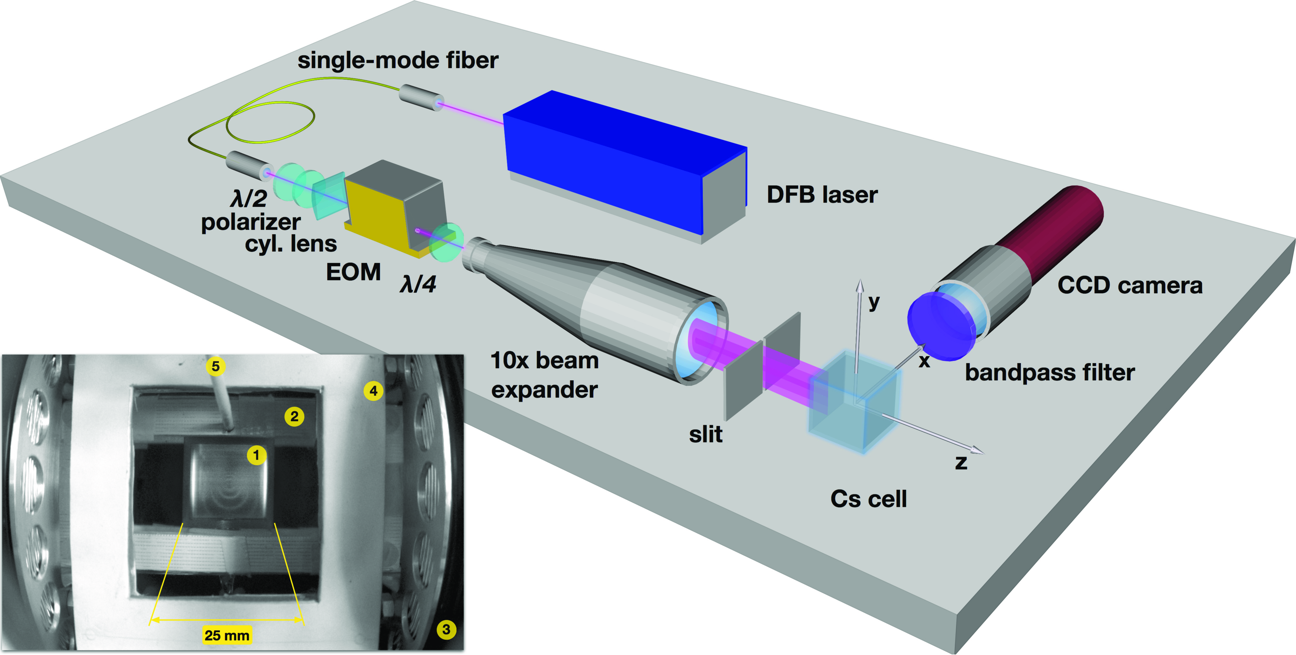
Figure 1: Schematic layout of the apparatus, not including magnetic field coils. The photograph shows the central part of the set-up, as seen by the CCD camera. One distinguishes: the cubic vapor cell (1) with ring-structured fluorescence produced by the 1WH field configuration, one of the support structures for the rf coils (2), the coils producing the quadrupole field (3), a support structure for the 8 wires of the 8W-configuration (4), and the protruding ‘wire’ of the 1WH field configuration.

In an auxiliary experiment we have determined the spin coherence relaxation rate in a transmission ground state Hanle experiment (similar to the one described by in Ref. [10]), yielding a 2 kHz (HWHM) linewidth. As discussed in Sec. 7, that linewidth becomes significantly narrower when the experiments are performed in a magnetically shielded environment.

Three mutually orthogonal pairs of (300${\times}$300 mm²) square Helmholtz coils were used to zero all components of the earth magnetic field. The rf field was produced by two rectangular (44${\times}$100 mm²) coils spaced by 22 mm driven by single sine wave or a superposition of sine waves delivered by a programmable (Keithley, model 3390) function generator. When using multi-component rf fields, we accounted for the frequency-dependent impedance of the rf-coil by giving the individual frequency components appropriate voltage amplitudes such as to deliver identical currents to the coils.

For the magnetic field mapping experiments reported below we have produced three types of inhomogeneous fields using three distinct coil and wire configurations as shown in Fig. 2.

4.1 Quadrupole ($Q$) field configuration

Two circular coils, are excited by identical currents of opposite sign, thus producing a quadrupole field that is well described by $\vec{B}(\vec{r})=B_{0}\,(x\,\hat{e}_{x}+y\,\hat{e}_{y}-2z\,\hat{e}_{z})$, with $\vec{r}=(x,y,z)$ over the cell dimension. The top graph of the left column in Fig. 2 shows the $Q$-configuration, together with the spectroscopy cell. The bottom of the same column shows the magnetic field lines represented by arrows in the $x=0$ plane (the plane imaged by the CCD camera looking along the $x$ direction), the arrow heads’ size representing the magnetic field strength.

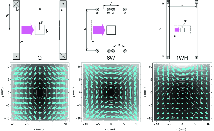
Figure 2: Top row: The three magnetic field configurations studied in this work, shown as cross sections in the $x{=}0$ plane. From left to right: Quadrupole (Q), eight wire (8W), and single wire plus Helmholtz (1WH) field configurations. The relative dimensions for each configuration are to scale, except for the wires ($w$) whose diameters are magnified 3 times. The cubic spectroscopy cell is located in the center of each coil arrangement The dashed rectangles represent the two rf-coils that are offset from the $x{=}0$ plane by $\pm$ 11 mm. The bottom row shows the calculated contour plots of the magnetic scalar potential in the spatial region covered by the cell, together with superimposed vector plots of the magnetic field lines in the $x=0$ plane.

The field lines are superposed on a contour plot of $|\vec{B}|$; the scalar magnetic equipotential surfaces being ellipsoids with aspect ratios $2{:}1$ in the $y{-}z$ and $x{-}z$ coordinates; the equipotential lines in the $x{=}0$ plane are thus ellipses with the same aspect ratio The characteristic feature of the $Q$-configuration are constant field gradients $dB_{z}/dz$ and $dB_{y}/dy$ with magnitudes in the ratio $-2{:}1$ along the $z$- and $y$-axes, respectively.

4.2 Eight-wire (8W) field configuration

Eight long wires arranged as shown in the top of the central column in Fig. 2 produce homogeneous gradients $dB_{y}/dz$ and $dB_{z}/dy$ of equal magnitude, as visualized by the field lines in the lower part of the figure. In the experimental set-up, the wires were 90 mm long copper rods. The iso-potential lines of the 8W-configuration in the $x{=}0$ plane in the vicinity of $y{=}0$ and $z{=}0$ are circles.

4.3 Helmholtz plus single wire (1WH) field configuration

The third field configuration consisted of two square coils in Helmholtz configuration, producing a homogeneous field along $\hat{z}$, onto which the field produced by a single current-carrying wire ($w$) along $\hat{x}$ is superposed. The sign of the wire current was chosen such as to compensate the homogeneous field at a point near the center of the cell. Such a field configuration, known as ‘z-wire trap’ is commonly used for the magnetic trapping of cold atoms on atom chips (see, e.g., [13]) since changing the relative magnitude of the wire and Helmholtz coil currents allows the controlled displacement of the zero field point along the vertical ($y$) direction. The coil configuration and a typical field pattern of its non-concentric potential lines are shown in the right column of Fig. 2.

4.4 Data recording and analysis

The laser-induced fluorescence from the irradiated Cs vapor layer was imaged by a 16-bit CCD camera (model ST-i monochrome from SBIG Astronomical Instruments, 640$\times$480 pixels), whose line-of-sight was directed along $\hat{x}$ (Figure 1). The zoom lens (ARBUS, model TV8553) was adjusted such that an area slightly larger than the (outer) 25${\times}$25 mm² cross section of the cell was imaged onto the CCD sensor. The LIF intensity variation of interest covered $\approx$10% of the 65’536 grey tones provided by the camera, because of bright regions of scattered light from the lateral windows, as can be seen in the photograph insert of Fig. 1. We note that with a conventional 8-bit camera that variation would cover only $\approx$25 shades of grey. An 894 nm interference filter mounted on the imaging lens suppressed stray room light.

The typical data recording procedures were as follows: In experiments involving depolarization by rf-irradiation we recorded two images with the same exposure time of typically 20–30 s, viz., one image (main image) with the magnetic field gradient and the rf-field applied to the cell, and one image (reference image) without applied rf-field. For recording the reference image the gradient field was switched off and replaced by a polarization stabilizing field $\beta_{\parallel}{\gg}1$, oriented along $\hat{k}$ for experiments on oriented atoms, and along the light polarization for experiments on aligned atoms. In an off-line analysis both images were cropped to display only the inner cell cross section of 22${\times}$22 mm², after which the reference image was subtracted from the main image. The grey tones in the difference image were then rescaled to span the full range from white to black by assigning 0 to the darkest pixel and 1 to the brightest pixel and mapping all intermediate grey tones in a linear manner onto the [0,1] interval.

Based on Eq. (6ka) the differential fluorescence image of oriented atoms is thus described by the expression

$$\delta P_{f}^{(1)}(\vec{r}) = P_{f}^{(1)}(\vec{r},S_{rf},\beta_{\parallel},\beta_{\perp})-P_{f}^{(1)}(\vec{r},S_{rf}{=}0,\beta_{\parallel}{\gg}1,\beta_{\perp}{=}0)$$ (6ko)

$$\propto C^{(1)}\left[\frac{1+\beta_{\parallel}^{2}(\vec{r})}{1+\beta_{\parallel}^{2}(\vec{r})+\beta_{\perp}^{2}(\vec{r})}\,\left(1-\frac{\sqrt{S_{rf}}}{[\beta_{rf}-\beta(\vec{r})]^{2}+S_{rf}+1}\right)\right],$$

where the local magnetic field components $\beta_{\parallel}$ and $\beta_{\perp}$, with $\beta{=}\sqrt{\beta_{\parallel}^{2}+\beta_{\perp}^{2}}$ of each voxel at position $\vec{r}$ in the imaged vapor layer determine the fluorescence intensity. Setting $C^{(1)}{=}1$ yields images with pixel intensities in the range $[0,1]$, the same range as covered by the experimental pictures.

In the same way, one derives for the differential fluorescence image of aligned atoms

$$\delta P_{f}^{(2)}(\vec{r}) = P_{f}^{(2)}(\vec{r},S_{rf},\beta_{\parallel},\beta_{\perp})-P_{f}^{(2)}(\vec{r},S_{rf}{=}0,\beta_{\parallel}{\gg}1,\beta_{\perp}{=}0)$$ (6kp)

$$\propto C^{(2)}\left[1{-}\left(\frac{1}{4}{+}\frac{3}{4}\frac{1{+}8\beta_{\parallel}^{2}{+}16\beta_{\parallel}^{4}}{1{+}4\beta_{\parallel}^{2}{+}4\beta_{\perp}^{2}}{-}3\frac{\beta_{\parallel}^{2}{+}\beta_{\parallel}^{4}}{1{+}\beta_{\parallel}^{2}{+}\beta_{\perp}^{2}}\right)\left(1{-}\frac{\sqrt{S_{rf}}}{(\beta_{rf}{-}\beta)^{2}{+}S_{rf}{+}1}\right)\right]\,,$$

where, as above, $C^{(2)}{=}1$ yields images with pixels values spanning the range from 0 (black) to 1 (white).

In the experiment described in Sec. 5.1 that did not use an rf magnetic field, the reference image was recorded by replacing the inhomogeneous magnetic field with a polarization-stabilizing longitudinal field $\beta_{\parallel}{\gg}1{\gg}\beta_{\perp}$. Using Eq. (6a), one easily sees that the difference image in that case is given by

$$\delta P_{f}^{(1)}(\vec{r}) = P_{f}^{(1)}(\vec{r},\beta_{\parallel},\beta_{\perp})-P_{f}^{(1)}(\vec{r},\beta_{\parallel}{\gg}1,\beta_{\perp}{=}0)$$ (6kq)

$$\propto \frac{\beta_{\perp}^{2}(\vec{r})}{1+\beta_{\parallel}^{2}(\vec{r})+\beta_{\perp}^{2}(\vec{r})}\,.$$

The experimental results in the following sections have been modeled by Eqs. (6ko–6kq), by adjusting only the rf saturation parameter $S_{rf}$ and the spin relaxation rate $\gamma$. In order to account for the inhomogeneous vertical intensity distribution of the laser beam in the cell, the theoretical fluorescence patterns in Eqs. (6ko–6kq) were multiplied by a Gaussian exp$[-y^{2}/2\sigma_{y}^{2}]$ with a FWHM of 15 mm.

5 Experimental results

5.1 Fluorescence of oriented atoms in inhomogeneous magnetic fields

The bottom row of Fig. 3 shows fluorescence images from the cell excited by circularly polarized light in the three inhomogeneous fields configurations described in Sec. 4. We refer to these fluorescence patterns as ‘Hanle background fluorescence’ images. The dark horizontal stripes on the fluorescence images are likely due to an interference effect from scattered laser light. Alternatively, the stripes could be shadows or reflections that are produced by small metallic Cs droplets on the windows of the cell.

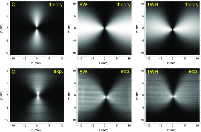
Figure 3: Two-dimensional fluorescence distributions induced by circularly polarized laser light in the three inhomogeneous field configurations shown in Fig. 2. From left to right: quadrupole field ($Q$), 8-wire field ($8W$), and Helmholtz plus one-wire field ($1WH$). The top row represents the LIF distribution calculated with Eq. (6a) and the lower row the experimentally recorded fluorescence patterns.

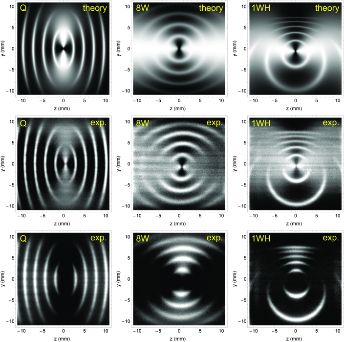
Figure 4: Magnetic resonance depolarization of fluorescence induced by circularly-polarized light in the three inhomogeneous field configurations. A multi-component rf-field is used space-selectively depolarizes the atoms, and the bright lines represent scalar magnetic iso-potential lines. For the $Q$- and the $1WH$- configurations the bright ellipses and circles represent–from inside to outside–lines along which the magnetic field modulus $\beta$ varies from 19 to 93 $\mu$T in steps of 18.5 $\mu$T. For the $8W$-configuration the corresponding fields were 10…50 $\mu$T (10 $\mu$T steps). The top row represents the LIF distributions predicted by Eq. (6ko) and the middle row the corresponding measured differential fluorescence patterns. The graphs in the bottom row were produced by subtracting a reference image recorded by switching off the rf field, while leaving the inhomogeneous field applied.

In the top row we show the corresponding modeled images predicted by Eq. (6kq) using the spatial field distributions $\beta_{\parallel}(\vec{r})$ and $\beta_{\perp}(\vec{r})$ of the three coil configurations, noting that the subscripts $\parallel$ and $\perp$ refer to the local magnetic field being parallel or perpendicular to the $\hat{k}$-vector of the exciting light beam. The observed and modeled fluorescence patterns show an excellent agreement, except near $\vec{r}=0$, where the dark spot is slightly less extended in the experimental images, a fact that we assign to laboratory field gradients, noting that, after all, the experiments are carried out in a magnetically unshielded environment. A small contribution from atomic alignment, not taken into account in our model, may also contribute to the slight deviation near $\vec{r}{=}0$.

5.2 Fluorescence of rf-depolarized oriented atoms in inhomogeneous magnetic field

Although the results presented in the previous paragraph show a good agreement between observations and the forward model predictions, they are not very useful for addressing the inverse problem that consists in inferring unknown magnetic field distributions from the fluorescence patterns that they produce.

As discussed in Sec. 3.2, the injection of a weak oscillating magnetic field (rf-field) into the cell is a powerful tool for addressing this inverse problem. Magnetic resonance transitions induced by the rf-field oscillating at $\omega_{rf}$ will depolarize atoms at locations where the magnetic resonance condition $\beta{=}|\vec{\beta}|{=}\sqrt{\beta_{\parallel}^{2}+\beta_{\perp}^{2}}{\equiv}\omega_{rf}/\gamma_{F}$ is fulfilled. This depolarization leads to an enhanced fluorescence intensity, thus highlighting regions of constant magnetic field strength ($\beta$=const), i.e., yielding bright scalar iso-potential lines. In order to demonstrate this approach we have exposed the cell to an rf-field consisting of a comb of 5 equidistant harmonic oscillations.

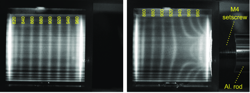
Figure 5: Potential lines in a region with a homogeneous field gradient (left) and deformation of the potential by an M4-setscrew (right).

For the $Q$- and the $1WH$- configurations the rf-field consisted of a fundamental oscillation at $\omega_{rf}/2\pi{=}$65 kHz and 4 harmonics thereof, while the measurements with the $8W$-field involved the fundamental and harmonics of 35 kHz. The graphs in the middle row of Fig. 4 show the experimental results, in which the bright iso-potential lines clearly stand out against the smooth Hanle background fluorescence pattern. The fluorescence predicted by Eq. (6ko) is shown in the top row of Fig. 4. The results in the top two rows were chosen to illustrate that our model calculations do not only reproduce the bright potential lines, but also the underlying Hanle background fluorescence patterns.

For practical applications one may wish to suppress the Hanle background. This can be achieved by recording the reference image with merely switching off the rf field, and leaving the inhomogeneous field applied. The corresponding results are shown in the bottom row of Fig. 4.

As an application we show in Fig. 5 the deformations of the potential lines by a magnetized stainless steel setscrew. The left graph shows a set of iso-field lines in a field produced by the superposition of the (homogeneous) field from a pair of Helmholtz coils and a small linear $dB_{z}/dz$-gradient field produced by the quadrupole coil $Q$. The rf-field for that measurement consisted of a superposition of oscillations at frequencies ranging from 820 to 960 kHz, yielding bright fluorescence lines at fields $B_{z}$ ranging from 234.3 to 274.3 $\mu$T, in steps of 5.7 $\mu$T.

When an M4 stainless steel setscrew held by a non-magnetic aluminum rod is approached to the cell from the right side, the iso-potential lines are displaced and deformed as shown on the right graph of Fig. 5. We show this example merely as a qualitative demonstration of the method. Work on quantitative methods for inferring the field produced by the perturbing object is in progress.

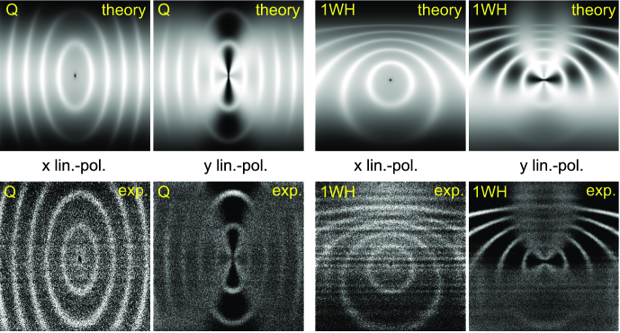
Figure 6: Magnetic resonance depolarization of fluorescence induced by linearly-polarized light in fields produced by the quadrupole ($Q$) and one wire plus Helmholtz ($1WH$) coils, respectively. Fluorescence images are shown for laser polarization parallel ($x$) and perpendicular ($y$) to the camera’s line of sight. A multi-component rf-field consisting of the fundamental and harmonics of 65 kHz is used to space-selectively depolarize atoms. The top row represents the LIF distributions calculated with Eq. (6kp) and the lower row the recorded differential fluorescence pattern.

5.3 Fluorescence from rf-depolarized aligned atoms in inhomogeneous magnetic field

We have also recorded fluorescence images induced by linearly-polarized light that creates an atomic alignment that is then resonantly destroyed by the rf-field in a space-selective manner. The use of linear polarization introduces an additional degree of freedom, viz., the relative orientation of the direction of polarization and the axis of symmetry (if any) of the gradient producing coils.

Results and their corresponding simulation based on Eq. (6kp) are shown in Fig. 6 for the quadrupole ($Q$) field and the one-wire plus Helmholtz ($1WH$) field. We find again an excellent agreement between the non-trivial simulated and measured patterns. We note in particular the dark spot in the zero-field point that is particularly well visible in the experiments with $x$-polarized light. We also note the poorer signal/noise ratio of the experimental data compared to the data obtained with circularly polarized light. This is due to the fact that the buffer gas reduces the optical pumping efficiency with linearly polarized light.

The dependence of the fluorescence maps on the orientation of the light polarization can be understood in a quantitave manner as follows. For the $Q$-configuration excited, e.g., with $y$-polarized light Fig. 2 shows that there is a growing alignment-stabilizing field $B_{y}$ along the $y$-direction, hence the dark band of growing width that develops as one moves away (along $y$) from the center of the cell. If, on the other hand, the light polarization (in the same $Q$-configuration) is along $x$, all field components in the imaged $x=0$ plane (except for the spot at $y{=}z{=}0$) have a depolarizing effect, hence the overall brighter image. Similar arguments allow one to understand the dark and bright zones in the $1WH$-configuration.

5.4 Dark resonance potential imaging by helicity-modulated light

In 1961 Bell and Bloom have shown [14] that a beam of intensity-modulated light induces magnetic resonance transitions in alkali atoms exposed to a transverse magnetic field when the modulation frequency matches the Larmor precession frequency. Recently we have extended the Bell-Bloom technique to polarization modulation [9, 15] in a transverse magnetic field. When the helicity $\xi$ of a circularly-polarized light beam is periodically reversed in synchronicity with the precession of the medium’s spin polarization, a resonant build-up of the polarization occurs when the modulation frequency $\omega_{mod}$ matches an integer multiple of the Larmor frequency $\omega_{L}$. This build-up manifest itself as a resonant reduction of the medium’s absorption coefficient when $\omega_{mod}=n\omega_{L}$, and hence a corresponding increase of the transmitted light power [15] .

!

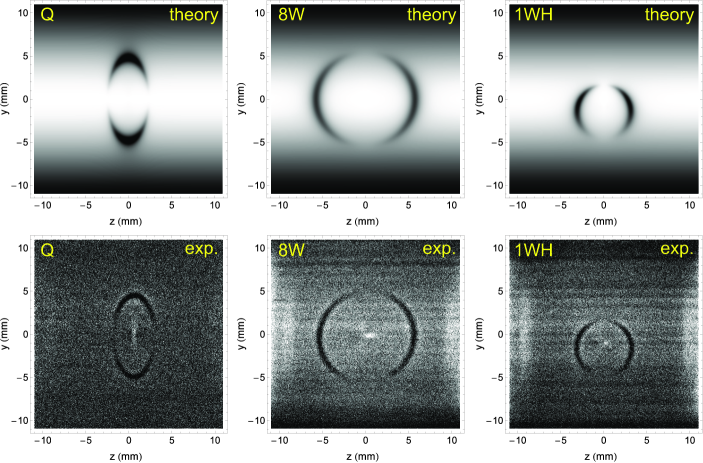
Figure 7: Fluorescence images showing a dark magnetic potential line (superposed on the Hanle background fluorescence) induced by the resonant creation of spin polarization using a light beam with circular polarization modulation. Experiments (bottom) were carried out in the three inhomogeneous field configurations $\nu_{mod}{=}$65 kHz in the $Q$- and $1WH$-fields, and 35 kHz in the $8W$-field. The top row shows the differential LIF distribution calculated by Eq. (6kr).

A reduction of the medium’s fluorescence is expected to go in pair with this variant of the EIT (electromagnetically-induced transparency) phenomenon. The graphs in the bottom row of Fig. 7 show fluorescence images recorded with circular polarization-modulated light in our three standard field configurations. In these recordings the reference image was recorded by switching off the polarization modulator, leaving the light in an unknown (i.e., unmeasured) elliptical polarization state. Since we did not (as for the recordings of Figs.4, 6) turn off the gradient field for recording the reference images, the Hanle fluorescence background is suppressed in the differential images.

The experimental images show well the anticipated dark potential line, at positions where the Larmor frequency matches the polarization modulation frequency. With $\omega_{mod}/2\pi{=}$65 kHz the dark line occurs at a field of 19 $\mu$T in the $Q$- and $1WH$-configurations, while it occurs at 10 $\mu$T in the $8W$-configuration for which $\omega_{mod}/2\pi$ was 35 kHz.

On notes the much poorer signal contrast of the (all-optical) modulation experiment compared to the experiments involving rf-depolarization that is partially due to the square-wave polarization modulation, of which only the fundamental Fourier component contributes. The graphs in the top row of of Fig. 7 show images that were modeled by the function

$$\delta P_{f}^{(1)}(\vec{r})\propto 1-\frac{\beta_{\parallel}^{2}(\vec{r})}{1+\beta_{\parallel}^{2}(\vec{r})+\beta_{\perp}^{2}(\vec{r})}\times\frac{1}{[\beta_{mod}-\beta(\vec{r})]^{2}+1}\,.$$ (6kr)

applied to all three gradient configurations. In the last expression we have retained only the fundamental Fourier component of the polarization modulation function, since the light intensity was too low to excite the harmonic resonances that are expected to occur at positions $\vec{r}$, where $\omega_{mod}=(n{>}1)\omega_{L}(\vec{r})$. These Bell-Bloom dark resonances are complementary to the bright resonances observed with rf-depolarization (Fig. 4).

6 Spatial resolution and magnetometric sensitivity of field mapping by fluorescence imaging

We estimate the spatial resolution $\Delta z$ of the iso-potential lines as follows: Suppose that spin-oriented atoms are in a local polarization stabilizing field, onto which a weak gradient field $G_{zz}{=}dB_{z}/dz$ is superposed. The interaction with the rf-field will then depolarize atoms, i.e., make the fluorescence light up in a region given by $\Delta z=\delta B/G_{zz}$, where $\delta B$ is the linewidth of the magnetic resonance line. Increasing the gradient $G_{zz}$ will narrow the iso-potential lines, until the region containing depolarized atoms broadens due to the depolarized atoms diffusing out of the depolarization region proper. In very strong gradients the spatial resolution will this be limited by the distance $\sqrt{2\,D\,\tau}$ over which depolarized atoms diffuse during their spin relaxation time $\tau$, $D$ being the diffusion constant. Since the two effects are statistically independent, we add them quadratically to obtain

$$\Delta z=\sqrt{2\,D\,\tau+\left(\delta B/G_{zz}\right)^{2}}\,.$$ (6ks)

We note that a similar approach was used by Tam [6], who added the two contributions linearly. Inspired by the latter work, we assume the spin relaxation rate to be given by

$$\Gamma=\tau^{-1}=\Gamma_{\mathrm{buffer}}+\Gamma_{\mathrm{pump}}+\gamma_{F}\,\delta B_{\mathrm{50Hz}}$$ (6kt)

where $\Gamma_{\mathrm{buffer}}$ is the depolarization rate due to collisions with buffer gas atoms, and $\Gamma_{\mathrm{pump}}$ the optical pumping, i.e., photon scattering rate. In our unshielded environment laboratory magnetic fields oscillating at the line frequency, artificially broaden the depolarization region, since they jiggle the region in which the rf-depolarization occurs by $\approx$1 mm, as shown below. We parametrize this effect in terms of $\delta B_{\mathrm{50Hz}}=\sqrt{\langle B^{2}(t)\rangle_{\mathrm{rms}}}$ and the corresponding broadening is one to two orders of magnitude larger than $\Gamma_{\mathrm{buffer}}$. Since the same broadening mechanism determines the width of the magnetic resonance line (an additional contribution from spin exchange collisions to the latter [6] being completely negligible), we can estimate the field gradient dependence of the spatial resolution to be given by

$$\Delta z\approx\sqrt{\frac{2\,D}{\gamma_{F}\,\delta B_{\mathrm{50Hz}}+\Gamma_{\mathrm{pump}}}+\left(\frac{\gamma_{F}\delta B_{\mathrm{50Hz}}+\Gamma_{\mathrm{pump}}}{G_{zz}}\right)^{2}}\,,$$ (6ku)

where it is reasonable to assume, although not explicitly proven, that optimal resolution conditions are achieved in the present configuration when $\Gamma_{\mathrm{pump}}$ is on the order of the 50 Hz broadening term.

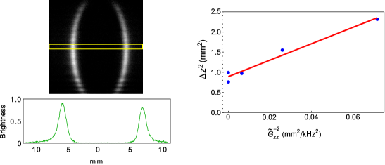
Figure 8: Dependence of the spatial resolution of the fluorescence field imaging method on the applied magnetic field gradient. Left: Typical fluorescence image with single rf-depolarization in $Q$-gradient field and intensity profile from data in yellow box above. Right: Gradient dependence of the profile widths, together with linear fit.

Figure 8 represents an experimental recording of the spatial resolution’s gradient dependence. For this measurement we varied the value of the gradient in the $Q$-configuration using a single harmonic oscillation whose frequency was adjusted to produce (for each gradient value) a single equipotential line, such as shown on the top left of Fig. 8 . Cuts through the fluorescence maps (bottom left part of the figure) were then used to infer the FWHM widths $\Delta z$ of the bright potential lines. The right graph of Fig. 8 shows the gradient dependence of $(\Delta z)^{2}$ together with a fit using the model function of Eq. (6ku). The intercept at strong gradients yields $\Delta z(G_{zz}{\rightarrow}\infty)$=0.94(4) mm. From the slope of the fitted line we infer an effective depolarization rate $\Gamma/2\pi$ of 4.5(2) kHz, a value that is compatible with the widths of magnetic resonance lines measured in an auxiliary double resonance transmission experiment.

We estimate the magnetometric resolution of the method in its current implementations as follows: The data in the cuts on the bottom left part of Fig. 8 represent fluorescence from a voxel of $\approx$ 1 mm³, whose signal/noise ratio $SNR$ is $\approx$ 400. We can thus state that the magnetometric sensitivity is $\delta B_{\mathrm{50Hz}}/\gamma_{F}/SNR\approx$ 2 nT with a recording time of 20 s.

7 Summary and outlook

We have presented a tomographic method for mapping two-dimensional distributions of magnetic scalar potentials that is based on the position-selective destruction of spin-polarization by magnetic resonance induced by a multi-component oscillating magnetic field. Potential lines are directly visible as CCD camera images, and their contrast can be enhanced by subtraction of suitable reference images. We have also presented algebraic equations that allow the easy forward modeling of the fluorescence pattern for three distinct current geometries used to produce easily calculable inhomogeneous magnetic fields.

The proof-of-principle experiments were carried out in an unshielded environment, where they yield a spatial resolution on the order of 1 mm. The resolution is limited by laboratory magnetic fields oscillating at the line frequency which broaden the magnetic resonance lines to a few kHz. In view of porting the experiments into a magnetically shielded environment we have already determined the magnetic resonance linewidth of the same cell to be on the order of 50 Hz, when recorded in a two-layer magnetic shield. Based on this we expect the spatial resolution to be given by $\Delta z=\sqrt{D/\Gamma_{\mathrm{pump}}}$, neglecting spin-exchange relaxation and assuming optimal detection conditions ($\Gamma_{\mathrm{pump}}{\approx}\Gamma_{\mathrm{buffer}}$). Based on this we believe that a spatial resolution on the order of 100 $\mu$m can be achieved when carrying out the experiments (using the same vapor cell) in a shielded environment. Work towards such measurements is in progress. In parallel we work on methods allowing the inverse reconstruction of spatially-resolved field patterns from sources with an unknown magnetization.

References

References

- [1] G. Alzetta, A. Gozzini, L. Moi, and G. Orriols. An experimental method for the observation of RF transitions and laser beat resonances in oriented Na vapour. Il Nuovo Cimento, 36 B(1):5–20, 1976.
- [2] J. Skalla, G. Wäckerle, M. Mehring, and A. Pines. Optical magnetic resonance imaging of Rb vapor in low magnetic fields. Physics Letters A, 226(1):69–74, 1997.
- [3] Kiyoshi Ishikawa, Yoshihiro Anraku, Yoshiro Takahashi, and Tsutomu Yabuzaki. Optical magnetic-resonance imaging of laser-polarized Cs atoms. Journal of the Optical Society of America B, 16(1):31, 1999.
- [4] D. Giel, G. Hinz, D. Nettels, and Antoine Weis. Diffusion of Cs atoms in Ne buffer gas measured by optical magnetic resonance tomography. Optics Express, 6(13):251–256, 2000.
- [5] A. C. Tam and W. Happer. Optically pumped cell for novel visible decay of inhomogeneous magnetic field or of rf frequency spectrum. Applied Physics Letters, 30(11):580, 1977.
- [6] A. C. Tam. Optical pumping of a dense Na+He+N2 system: Application as an rf spectrum analyzer. Journal of Applied Physics, 50(3):1171, 1979.
- [7] Hitoshi Asahi, Koji Motomura, Ken-ichi Harada, and Masaharu Mitsunaga. Dark-state imaging for two-dimensional mapping of a magnetic field. Optics Letters, 28(13):1153–5, 2003.
- [8] E. E. Mikhailov, I. Novikova, M. D. Havey, and F. A. Narducci. Magnetic field imaging with atomic Rb vapor. Optics Letters, 34:3529–3531, 2009.
- [9] Zoran D. Grujić and Antoine Weis. Atomic magnetic resonance induced by amplitude-, frequency-, or polarization-modulated light. Physical Review A, 88(1):012508, 2013.
- [10] Natasha Castagna and Antoine Weis. Measurement of longitudinal and transverse spin relaxation rates using the ground-state Hanle effect. Physical Review A, 84(5):053421, 2011.
- [11] Evelina Breschi and Antoine Weis. Ground-state Hanle effect based on atomic alignment. Physical Review A, 86(5):053427, 2012.
- [12] F. Bloch. Nuclear Induction. Physical review, 70:460–474, 1946.
- [13] Ron Folman, Peter Krüger, Jörg Schmiedmayer, Johannes Denschlag, and Carsten Henkel. Microscopic atom optics: From wires to an atom chip. volume 48 of Advances In Atomic, Molecular, and Optical Physics, pages 263––356. Academic Press, 2002.
- [14] William E. Bell and Arnold L. Bloom. Observation of forbidden resonances in optically driven spin systems. Physical Review Letters, 6(11):623–624, 1961.
- [15] Ilja Fescenko, Paul Knowles, Antoine Weis, and Evelina Breschi. A Bell-Bloom experiment with polarization-modulated light of arbitrary duty cycle. Optics Express, 21(13):15121, 2013.