Sampling-based Roadmap Planners are Probably Near-Optimal after Finite Computation

Abstract

Sampling-based motion planners have proven to be efficient solutions to a variety of high-dimensional, geometrically complex motion planning problems with applications in several domains. The traditional view of these approaches is that they solve challenges efficiently by giving up formal guarantees and instead attain asymptotic properties in terms of completeness and optimality. Recent work has argued based on Monte Carlo experiments that these approaches also exhibit desirable probabilistic properties in terms of completeness and optimality after finite computation. The current paper formalizes these guarantees. It proves a formal bound on the probability that solutions returned by asymptotically optimal roadmap-based methods (e.g., ${\tt PRM}^{*}$) are within a bound of the optimal path length $I_{\epsilon_{n}}^{*}$ with clearance $\epsilon_{n}$ after a finite iteration $n$. This bound has the form $\mathbb{P}\big{(}|I_{n}-I_{\epsilon_{n}}^{*}|\leq\delta\cdot I_{\epsilon_{n}}^{*}\big{)}\leq\mathbb{P}_{success}$, where $\delta$ is an error term for the length a path in the ${\tt PRM}^{*}$ graph, $I_{n}$. This bound is proven for general dimension Euclidean spaces and evaluated in simulation. A discussion on how this bound can be used in practice, as well as bounds for sparse roadmaps are also provided.

1 Background

Early contributions in sampling-based motion planning focused on overcoming the computational challenges posed by motion planning problems with high dimensionality and geometrically complex spaces Latombe (1991); LaValle (2006); Choset et al. (2005). Two alternative families of sampling based planners emerged during this process, roadmap-based methods, such as $\tt PRM$Kavraki et al. (1996); Kavraki and Latombe (1998), which are suited to multi-query planning, and tree-based approaches, such as ${\tt RRT}$LaValle (1998); LaValle and Kuffner (2000). Formal analysis of these methods followed, showing they are probabilistically complete Kavraki et al. (1998); Hsu et al. (1998); Ladd and Kavraki (2004); Chaudhuri and Koltun (2009). Though these methods are probabilistically complete, the literature has shown that solution non-existence can be detected under certain conditions Varadhan and Manocha (2005); McCarthy et al. (2012). Other work tries to return high clearance paths, or characterize the $\mathcal{C}$-space obstacles Wilmarth et al. (1999); Amato et al. (1998), and others return high quality solutions in practice Raveh et al. (2011).

A major recent breakthrough was the identification of the conditions under which these methods asymptotically converge to optimal paths Karaman and Frazzoli (2011, 2010), resulting in algorithms such as ${\tt RRT}^{*}$and ${\tt PRM}^{*}$. Both probabilistic completeness and asymptotic optimality relate to desirable properties after infinite computation time. Since these methods are practically terminated after some finite amount of computation, these guarantees cannot provide information about expected path cost or of solution non-existence in practice Varadhan and Manocha (2005); McCarthy et al. (2012). Nevertheless, experiments show that asymptotically optimal methods do have very good behavior in terms of path quality after finite computation time, even when optimality constraints are relaxed to create more efficient methods with path length guarantees Marble and Bekris (2013); Salzman and Halperin (2013); Wang et al. (2013). To address the gap between practical experience and formal guarantees, recent work by the authors has proposed that asymptotically optimal sampling-based planners also exhibit probabilistic near-optimality properties after finite computation using Monte Carlo experiments Dobson and Bekris (2013). This kind of guarantee is similar to the concept of Probably Approximately Correct (${\tt PAC}$) solutions in the machine learning literature Valiant (1984). The focus in this work is on the properties of roadmap-based methods, such as ${\tt PRM}^{*}$, as they are easier to analyze.

This work formally shows the Probabilistic Near-Optimality (${\tt PNO}$) of sampling-based roadmap methods in general settings and with limited assumptions. It provides the following contributions relative to the state-of-the-art and the previous contribution by the authors Dobson and Bekris (2013):

• Prior work relied on Monte Carlo simulations to provide path length bounds, while this work achieves tight, closed-form bounds. This required solving a problem in geometric probability, which to the best of the authors’ knowledge had not been addressed before.

• The framework is extended to work with a version of ${\tt PRM}^{*}$ which constructs a roadmap having $O(n\log{n})$ edges, which is in the order of the lower bound for asymptotic optimality. Prior work used a method called ${\tt PNO}\text{-}{\tt PRM^{*}}$, which creates $O(n^{2})$ edges.

2 Problem Setup

This section introduces terminology and definitions required for the formal analysis. This work examines kinematic planning in the configuration space, $\mathcal{C}$, where a robot’s configuration $q\in\mathcal{C}_{\text{free}}$ is cast as a point. $\mathcal{C}$ is partitioned into the collision free ($\mathcal{C}_{\text{free}}$) and colliding ($\mathcal{C}_{\text{obs}}$) configurations. This work reasons over $\mathcal{C}$ as a metric space, using the Euclidean $L_{2}$-norm as a distance metric. The objective is to compute a path $\pi_{n}:[0,1]\to\mathcal{C}_{\text{free}}$ after finite iterations $n$ with path length guarantees relative to an $\epsilon$-robust feasible path, i.e. a path with minimum distance to $\mathcal{C}_{\text{obs}}$ of at least $\epsilon$. If a motion planning problem is robustly feasible, there exists a set of $\epsilon$-robust paths which answer a query, $(q_{start},q_{goal})$. Let the path of minimum length from the set be denoted as $\pi^{*}_{\epsilon_{n}}$, with length $I_{\epsilon_{n}}^{*}$. The path planning problem this work considers is the following:

Defn. 1 (Robustly Feasible Motion Planning)

Let the tuple $(\mathcal{C},q_{start},q_{goal},{\epsilon_{0}})$ be an instance of a Robustly Feasible Motion Planning Problem. Given a configuration space $\mathcal{C}$, two configurations $q_{start}$, $q_{goal}\in\mathcal{C}_{\text{free}}\subset\mathcal{C}$ and a clearance value ${\epsilon_{0}}$ so that an ${\epsilon_{0}}$-robust path $\pi_{{\epsilon_{0}}}$ exists so that $\pi_{{\epsilon_{0}}}(0)=q_{start}$ and $\pi_{{\epsilon_{0}}}(0)=q_{goal}$, find a solution path $\pi$ so that $\pi(0)=q_{start}$ and $\pi(1)=q_{goal}$.

To solve this problem, a slight variation of the ${\tt PRM}^{*}$ algorithm is applied Karaman and Frazzoli (2011). The high-level operations of ${\tt PRM}^{*}$ are as follows:

• ${\tt PRM}^{*}$ generates configurations $Q$ in $\mathcal{C}_{\text{free}}$, rejecting samples generated in $\mathcal{C}_{\text{obs}}$, and then adding $Q$ to a graph, $G=(V,E)$, i.e. $V\leftarrow V\cup Q$.

• For each sample, an $r_{n}$ radius, where $r_{n}=\gamma_{{\tt PRM}^{*}}\cdot\Big{(}\frac{\ln{n}}{n}\Big{)}^{\frac{1}{d}}$ Karaman and Frazzoli (2011), local neighborhood in $\mathcal{C}_{\text{free}}$ is examined. If a local path to a neighbor can be generated which remains entirely in $\mathcal{C}_{\text{free}}$, an edge connecting them is added to $E$.

• The above steps are repeated iteratively until some stopping criterion is met.

This work’s variant ${\tt PRM}^{*}$ uses a larger connection radius, $\gamma_{{\tt PNO}}=2\cdot\gamma_{{\tt PRM}^{*}}$, and the reason why becomes apparent from the analysis. The larger connection radius allows for the following property to be argued:

Prop. 1 (Probabilistic Near-Optimality for RFMP)

An algorithm $ALG$ is probabilistically near-optimal for an RFMP problem $(\mathcal{C},q_{start},q_{goal},{\epsilon_{0}})$, if for a finite iteration $n>n_{0}$ of $ALG$ and a given error threshold $\delta$, it is possible to compute a probability $\mathbb{P}_{success}$ so that for the length $I_{n}$ of a path $\pi_{n}$ answering the query in the planning structure computed by $ALG$ at iteration $n$:

$$\mathbb{P}(|I_{n}-I_{\epsilon_{n}}^{*}|>\delta\cdot I_{\epsilon_{n}}^{*})<1-\mathbb{P}_{success}$$

where $I_{\epsilon_{n}}^{*}$ is the length of the optimum $\epsilon_{n}$-robust path $\pi^{*}_{\epsilon_{n}}$ for a value $\epsilon_{n}<{\epsilon_{0}}$.

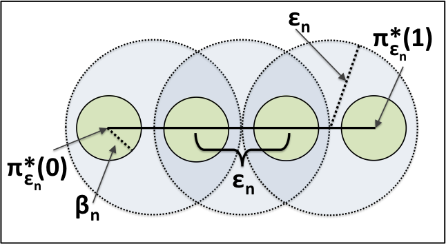
Figure 1: Hyperballs over an optimal path with radius $\beta_{n}$ and separation $\epsilon_{n}$. Consecutive balls lie entirely within some clearance ball $\mathcal{B}_{\epsilon_{n}}(\pi^{*}_{\epsilon_{n}}(\tau_{t}))$.

The clearance of the optimum path $\epsilon_{n}$ considered at iteration $n$ and the iteration $n_{0}$ after which point the guarantee can be achieved, can be computed given the analysis in this work.

Probabilistic Near-Optimality (${\tt PNO}$) can be argued by reasoning over a theoretical construction of hyperballs tiled over $\pi^{*}_{\epsilon_{n}}$, where hyperballs are denoted as $\mathcal{B}_{r}(q_{c})$, being centered at configuration $q_{c}$ and having radius $r$. The construction of these hyperballs is illustrated in Figure 1. Construct $M_{n}+1={\lceil\frac{I_{\epsilon_{n}}^{*}}{\epsilon_{n}}\rceil}+1$ balls, $B_{n}$ centered along $\pi^{*}_{\epsilon_{n}}$, i.e. $B_{n}=\{\mathcal{B}_{\beta_{n}}(\pi^{*}_{\epsilon_{n}}(\tau_{0})),\ldots,\mathcal{B}_{\beta_{n}}(\pi^{*}_{\epsilon_{n}}(\tau_{M_{n}}))\}$, having radius $\beta_{n}\leq\frac{1}{2}\epsilon_{n}$, where $\epsilon_{n}=\frac{1}{2}r_{n}$, and where $r_{n}$ is the connection radius used by the algorithm. The construction enforces the centers of the balls to be $\epsilon_{n}$ apart, and by choice of $\beta_{n}$, these balls have empty intersections. Then, since $r_{n}\geq 4\beta_{n}$, the algorithm will attempt connections between any pairs of points between consecutive hyperballs. ${\tt PNO}$ guarantees are over a path in the planning structure with length $I_{n}$. This path corresponds to the set of all the first samples generated in each of the hyperballs.

Then, using the steps from related work Karaman and Frazzoli (2011), $\gamma_{\tt PNO}$ can be derived, as well as, $k(n)$ for an equivalent ${\tt k}\text{-}{\tt PRM}^{*}$ variant. These values are derived in the next section.

3 Derivation

This section provides a bound on the probability that ${\tt PRM}^{*}$ returns poor-quality paths. Namely, it constructs the probability of $I_{n}$ being $1+\delta$ times larger than the optimal path after $n$ iterations. Then, it provides a guarantee $\mathbb{P}(|I_{n}-I_{\epsilon_{n}}^{*}|>\delta\cdot I_{\epsilon_{n}}^{*})<1-\mathbb{P}_{success}$, where $\delta>0$ is an input multiplicative bound, and $\mathbb{P}_{success}\in(0,1)$ is a confidence bound. A guarantee of this type can be considered a Probably Near Optimal (${\tt PNO}$) property. First, the algorithmic parameters $\gamma_{\tt PNO}$ and $k(n)$ are derived.

3.1 Deriving $\gamma_{\tt PNO}$

This section employs the same steps as the derivation for $\gamma_{{\tt PRM}^{*}}$ in the literature Karaman and Frazzoli (2011). The objective of this section is to leverage a bound on the probability that ${\tt PRM}^{*}$ will fail to produce a sample in each of the hyperballs over $\pi^{*}_{\epsilon_{n}}$ to derive an appropriate constant for the connection radius. Let this connection radius employed by the ${\tt PRM}^{*}$ variant be $r_{n}=\gamma_{\tt PNO}\Big{(}\frac{\ln{n}}{n}\Big{)}^{\frac{1}{d}}$. Then, by construction, this connection radius is at least four times larger than the radius of a hyperball, i.e. $\beta_{n}<\frac{1}{4}\gamma_{\tt PNO}\Big{(}\frac{\ln{n}}{n}\Big{)}^{\frac{1}{d}}$. Then,

$$|\mathcal{B}_{\beta_{n}}|=V_{d}\beta_{n}^{d}<V_{d}\big{(}\frac{r_{n}}{4}\big{)}^{d}=V_{d}\cdot\frac{\ln{n}}{n}\big{(}\frac{\gamma_{\tt PNO}}{4}\big{)}^{d},$$

where $V_{d}=|\mathcal{B}_{1}|$ is the $d$-dimensional constant for the volume of a hyperball. Also by construction, $\epsilon_{n}\geq\frac{1}{2}\gamma_{\tt PNO}\Big{(}\frac{\ln{n}}{n}\Big{)}^{\frac{1}{d}}$. Then, the number of hyperballs constructed over $\pi^{*}_{\epsilon_{n}}$ can be bounded by $M_{n}\leq\frac{I_{\epsilon_{n}}^{*}}{\epsilon_{n}}=\frac{2I_{\epsilon_{n}}^{*}}{\gamma_{\tt PNO}}\Big{(}\frac{n}{\ln{n}}\Big{)}^{\frac{1}{d}}$.

Then, in line with previous work in the literature Kavraki et al. (1998); Karaman and Frazzoli (2011), the probability of failure can be bounded using the probability that a single hyperball contains no sample. The event that a single hyperball does not contain a sample is denoted as $\mathcal{F}$, and has probability:

$$\mathbb{P}(\mathcal{F})=\bigg{(}1-\frac{|\mathcal{B}_{\beta_{n}}|}{|\mathcal{C}_{\text{free}}|}\bigg{)}^{n}<\bigg{(}1-\frac{V_{d}}{|\mathcal{C}_{\text{free}}|}\cdot\frac{\ln{n}}{n}\cdot\Big{(}\frac{\gamma_{\tt PNO}}{4}\Big{)}^{d}\bigg{)}^{n}$$

Then, since $(1-x)^{t}\leq e^{-tx}$,

$$\mathbb{P}(\mathcal{F})\leq e^{-\frac{V_{d}}{|\mathcal{C}_{\text{free}}|}\cdot\ln{n}\cdot\big{(}\frac{\gamma_{\tt PNO}}{4}\big{)}^{d}}=n^{-\frac{V_{d}}{|\mathcal{C}_{\text{free}}|}\cdot\big{(}\frac{\gamma_{\tt PNO}}{4}\big{)}^{d}}$$ (1)

Now, compute bounds on the event $\Omega^{C}$ that at least one ball does not contain a sample as:

$$\mathbb{P}(\Omega^{C})=\mathbb{P}\big{(}\bigcup_{M_{n}}\mathcal{F}\big{)}\leq\sum_{i=1}^{M_{n}}\mathbb{P}(\mathcal{F})=(M_{n})\mathbb{P}(\mathcal{F})$$

Substituting the computed value for $M_{n}$, and $\mathbb{P}(\mathcal{F})$ from Eq. 1:

$$\mathbb{P}(\Omega^{C})\leq\bigg{(}\frac{2I_{\epsilon_{n}}^{*}}{\gamma_{\tt PNO}}\Big{(}\frac{n}{\ln{n}}\Big{)}^{\frac{1}{d}}\bigg{)}n^{-\frac{V_{d}}{|\mathcal{C}_{\text{free}}|}\cdot\big{(}\frac{\gamma_{\tt PNO}}{4}\big{)}^{d}}=\\ \bigg{(}\frac{2I_{\epsilon_{n}}^{*}}{\gamma_{\tt PNO}}\frac{1}{(\ln{n})^{\frac{1}{d}}}\bigg{)}n^{-\big{(}\frac{V_{d}}{|\mathcal{C}_{\text{free}}|}\cdot\big{(}\frac{\gamma_{\tt PNO}}{4}\big{)}^{d}-\frac{1}{d}\big{)}}$$

Now, if $\sum_{i=1}^{\infty}\mathbb{P}(\Omega^{C})$ is less than infinity, this implies by the Borel-Cantelli theorem that $\mathbb{P}(\limsup_{n\to\infty}\Omega^{C})=0$ Grimmet and Stirzaker (2001). Furthermore, by the Zero-one Law, $\mathbb{P}(\limsup_{n\to\infty}\Omega^{C})=0\Rightarrow\mathbb{P}(\limsup_{n\to\infty}\Omega_{n}^{\beta})=1$, meaning the probability of coverage converges to $1$ in the limit.

In order for the sum to be less than infinity, it is sufficient to show that the exponent, $\frac{V_{d}}{|\mathcal{C}_{\text{free}}|}\cdot\big{(}\frac{\gamma_{\tt PNO}}{4}\big{)}^{d}-\frac{1}{d}<1$. The algorithm can ensure this by using an appropriate value of $\gamma_{\tt PNO}$. Solving the inequality for $\gamma_{\tt PNO}$ shows that it suffices that:

$$\gamma_{\tt PNO}>4\bigg{(}\Big{(}1+\frac{1}{d}\Big{)}\Big{(}\frac{|\mathcal{C}_{\text{free}}|}{V_{d}}\Big{)}\bigg{)}^{\frac{1}{d}}$$

3.2 Deriving $k(n)$ for ${\tt k}\text{-}{\tt PRM}^{*}$

This section employs the same steps as the derivation for $k(n)$ in the literature Karaman and Frazzoli (2011). The objective of this section is to derive the function, $k(n)$, for a ${\tt PNO}$ variant of ${\tt k}\text{-}{\tt PRM}^{*}$. The high-level idea is that it will be shown that two events happen infinitely often with the given $k(n)$; the set of hyperballs each contain at least one sample, and that each ball of radius $\epsilon_{n}$ has no more than $k(n)$ samples inside it. From this, it is clear that if ${\tt k}\text{-}{\tt PRM}^{*}$ attempts to connect each sample with $k(n)$ neighbors, it will attempt connections between samples in neighboring hyperballs.

Then, using the computed value of $\gamma_{\tt PNO}$ from above,

$$M_{n}\leq\frac{1}{2}I_{\epsilon_{n}}^{*}\bigg{(}\Big{(}\frac{V_{d}}{|\mathcal{C}_{\text{free}}|}\Big{)}\Big{(}\frac{n}{\ln{n}}\Big{)}\Big{(}\frac{1}{1+\frac{1}{d}}\Big{)}\bigg{)}^{\frac{1}{d}},\text{ and }\\ |\mathcal{B}(\epsilon_{n})|\leq\Big{(}V_{d}\cdot 4^{d}\Big{)}\Big{(}\frac{1}{2}\Big{)}^{d}\Big{(}1+\frac{1}{d}\Big{)}\Big{(}\frac{|\mathcal{C}_{\text{free}}|\ln{n}}{nV_{d}}\Big{)}=\\ 2^{d}\Big{(}1+\frac{1}{d}\Big{)}\Big{(}\frac{|\mathcal{C}_{\text{free}}|\ln{n}}{n}\Big{)}$$

Let $A$ be an indicator random variable which takes value $1$ when there is a sample in some arbitrary hyperball of radius $\epsilon_{n}$. Then, $\mathbb{E}[A]=\frac{|\mathcal{B}(\epsilon_{n})|}{|\mathcal{C}_{\text{free}}|}=2^{d}(1+\frac{1}{d})(\frac{\ln{n}}{n})$. Since each sample is drawn independently of the others, the number of samples in a ball can be expressed as a random variable $N$, such that $\mathbb{E}[N]=n\mathbb{E}[A]=2^{d}(1+\frac{1}{d})\ln{n}$. Due to $A$ being a Bernoulli random variable, the Chernoff Bound can be employed to bound the probability of $N$ taking large values, namely:

$$\mathbb{P}(N>(1+t)\mathbb{E}[N])\leq\bigg{(}\frac{e^{t}}{(1+t)^{(1+t)}}\bigg{)}^{\mathbb{E}[N]},t>0$$

Then, let $t=e-1$. Substituting this above yields:

$$\mathbb{P}(N>e\mathbb{E}[N])\leq e^{-\mathbb{E}[N]}=e^{-2^{d}(1+\frac{1}{d})\ln{n}}=n^{-2^{d}(1+\frac{1}{d})}$$

Now, in order for the $k(n)$ connections to attempt connections outside of a $\epsilon_{n}$-ball, it must be that:

$$k(n)=k_{\tt PNO}e\Big{(}1+\frac{1}{d}\Big{)}\geq 2^{d}e\Big{(}1+\frac{1}{d}\Big{)}=e\mathbb{E}[N],$$

which clearly holds if $k_{\tt PNO}=2^{d}$. This implies that $\mathbb{P}(N>k(n))\leq n^{-2^{d}(1+\frac{1}{d})}$.

Finally, consider the event $\zeta$ that even one of the balls has more than $k(n)$ samples:

$$\mathbb{P}(\zeta)=\mathbb{P}\Big{(}\bigcup_{M_{n}}\mathbb{P}(N>k(n))\Big{)}\leq\\ \sum^{M}_{n}\mathbb{P}(N>k(n))=M_{n}\mathbb{P}(N>k(n))$$

$$\mathbb{P}(\zeta)\leq\frac{I_{\epsilon_{n}}^{*}}{2}\bigg{(}\frac{V_{d}}{\ln{n}|\mathcal{C}_{\text{free}}|(1+\frac{1}{d})}\bigg{)}^{\frac{1}{d}}n^{-2^{d}(1+\frac{1}{d})+\frac{1}{d}}$$

Then, it is clear that $\sum_{i=1}^{\infty}\mathbb{P}(\zeta)<\infty$, which by the Borel-Cantelli Theorem implies that $\mathbb{P}(\limsup_{n\to\infty}\zeta)=0$, and furthermore, $\mathbb{P}(\limsup_{n\to\infty}\zeta^{C})=1$ via the Zero-one Law, i.e. the number of samples in the $\epsilon_{n}$-ball is almost certainly less than $k(n)$.

Finally, using the result showing the convergence of $\mathbb{P}(\Omega_{n}^{\beta})$ to $1$, and the above result for $\mathbb{P}(\zeta^{C})$, it can be concluded that $\mathbb{P}(\limsup_{n\to\infty}(\Omega_{n}^{\beta}\cap\zeta^{C}))=1$, implying that for the choice of $k(n)$, ${\tt k}\text{-}{\tt PRM}^{*}$ attempts the appropriate connections.

3.3 Deriving the Probability of Coverage

The derivation of the probability of path coverage leverages several results in the literature Kavraki et al. (1998); Karaman and Frazzoli (2011); Dobson and Bekris (2013). The objective is to exactly derive the probability that at any finite iteration, $n$, the algorithm has generated a sample in each of the hyperballs over $\pi^{*}_{\epsilon_{n}}$. Deriving this probability will work off of the result shown in prior work which gives the probability of coverage for a similar construction of hyperballs to that employed here Dobson and Bekris (2013), which shows:

$$\mathbb{P}(\Omega_{n}^{\beta})=\bigg{(}1-\Big{(}1-\frac{|\mathcal{B}_{\beta}|}{|\mathcal{C}_{\text{free}}|}\Big{)}^{n}\bigg{)}^{M+1},$$ (2)

where $\beta$ is the radius of the set of hyperballs and $M+1$ is the number of such hyperballs. Here, the inner term $\Big{(}1-\frac{|\mathcal{B}_{\beta}|}{|\mathcal{C}_{\text{free}}|}\Big{)}^{n}$ is the probability of failing to throw a sample in a particular hyperball after $n$ samples have been thrown. Then, the probability of success for throwing a sample in all of the hyperballs yields the above form. This holds for any values of $\beta$ and $M$ such that the hyperballs are disjoint, which is exactly the construction employed in this work. Then, substituting the values computed for $\beta_{n}$ and $M_{n}$ from Section 3.1 above yields:

$$\mathbb{P}(\Omega_{n}^{\beta})\approx\bigg{(}1-\Big{(}1-a\Big{)}^{n}\bigg{)}^{{\frac{1}{2}I_{\epsilon_{n}}^{*}\Big{(}b\Big{)}^{-\frac{1}{d}}}+1}$$

where $a=\frac{V_{d}\Big{(}{\sqrt[d]{\big{(}1+\frac{1}{d}\big{)}\big{(}\frac{|\mathcal{C}_{\text{free}}|\ln{n}}{V_{d}n}\big{)}}}\Big{)}^{d}}{|\mathcal{C}_{\text{free}}|}$, $b=\big{(}1+\frac{1}{d}\big{)}\big{(}\frac{|\mathcal{C}_{\text{free}}|\ln{n}}{V_{d}n}\big{)}$, and $V_{d}$ is the d-dimensional constant for the volume of a hyperball, i.e. $|\mathcal{B}(r)|=V_{d}r^{d}$. Then, simplifying this expression yields the following Lemma:

Lemma 1 (Probability of Path Coverage)

Let $\Omega_{n}^{\beta}$ be the event that for one execution of ${\tt PRM}^{*}$  there exists at least one sample in each of the $M_{n}+1$ hyperballs of radius $\beta_{n}$ over the clearance robust optimal path, $\pi^{*}_{\epsilon_{n}}$, for a specific value of $n>n_{0}$ and $\beta_{n}$. Then,

$$\mathbb{P}(\Omega_{n}^{\beta})\approx\bigg{(}1-\Big{(}1-a\Big{)}^{n}\bigg{)}^{\frac{1}{2}I_{\epsilon_{n}}^{*}\big{(}b\big{)}^{-\frac{1}{d}}+1}$$ (3)

Where $a=\Big{(}1+\frac{1}{d}\Big{)}\Big{(}\frac{\log{n}}{n}\Big{)}$ and $b=\Big{(}1+\frac{1}{d}\Big{)}\Big{(}\frac{|\mathcal{C}_{\text{free}}|\log{n}}{V_{d}n}\Big{)}$.

3.4 Deriving a probabilistic bound

Let $\Omega^{C}$ be the event that there does not exist a sample in each of the hyperballs covering a path, i.e. $\mathbb{P}(\Omega^{C})=1-\mathbb{P}(\Omega_{n}^{\beta})$. Then, the value for $\mathbb{P}(|I_{n}-I_{\epsilon_{n}}^{*}|>\delta\cdot I_{\epsilon_{n}}^{*})$ can be expressed as:

$$\mathbb{P}\big{(}|I_{n}-I_{\epsilon_{n}}^{*}|>\delta\cdot I_{\epsilon_{n}}^{*}\ |\ \Omega_{n}^{\beta}\big{)}\mathbb{P}(\Omega_{n}^{\beta})\\ +\mathbb{P}\big{(}|I_{n}-I_{\epsilon_{n}}^{*}|>\delta\cdot I_{\epsilon_{n}}^{*}\ |\ \Omega^{C}\big{)}\mathbb{P}(\Omega^{C})$$

This is because the probability of returning a low quality path is expressed as a sum of probabilities, when event $\Omega_{n}^{\beta}$ has occurred, and when $\Omega_{n}^{\beta}$ has not occurred. Since $\mathbb{P}(\Omega^{C})=1-\mathbb{P}(\Omega_{n}^{\beta})$, then via Lemma 1, both $\mathbb{P}(\Omega^{C})$ and $\mathbb{P}(\Omega_{n}^{\beta})$ are known for known $n$ and $\beta$. It is assumed that the probability of a path being larger than $\delta$ is quite high if $\Omega_{n}^{\beta}$ has not happened, i.e. $\mathbb{P}\big{(}|I_{n}-I_{\epsilon_{n}}^{*}|>\delta\cdot I_{\epsilon_{n}}^{*}\ |\ \Omega^{C}\big{)}$ is close to $1$; therefore, this probability can be upper bounded by $1$. All that remains is to compute $\mathbb{P}\big{(}|I_{n}-I_{\epsilon_{n}}^{*}|>\delta I_{\epsilon_{n}}^{*}\ |\ \Omega_{n}^{\beta}\big{)}$. Let $y$ be a random variable identically distributed with $I_{n}$, but having $0$ mean, i.e. $y=I_{n}-\mathbb{E}[I_{n}]$. Then, let

$$\mathbb{P}\big{(}|I_{n}-I_{\epsilon_{n}}^{*}|>\delta I_{\epsilon_{n}}^{*}\ |\ \Omega_{n}^{\beta}\big{)}=\\ \mathbb{P}\big{(}|\mathbb{E}[I_{n}]+y-I_{\epsilon_{n}}^{*}|>\delta I_{\epsilon_{n}}^{*}\ |\ \Omega_{n}^{\beta}\big{)}$$

Then, the absolute value can be removed, as $|X|>a\Rightarrow X>a$ or $X<-a$. Then, the probability is equal to the sum:

$$\mathbb{P}\big{(}\mathbb{E}[I_{n}]+y-I_{\epsilon_{n}}^{*}>\delta I_{\epsilon_{n}}^{*}\ |\ \Omega_{n}^{\beta}\big{)}\\ +\mathbb{P}\big{(}\mathbb{E}[I_{n}]+y-I_{\epsilon_{n}}^{*}<-\delta I_{\epsilon_{n}}^{*}\ |\ \Omega_{n}^{\beta}\big{)},$$

where due to symmetry,

$$\mathbb{P}\big{(}|I_{n}-I_{\epsilon_{n}}^{*}|>\delta I_{\epsilon_{n}}^{*}\ |\ \Omega_{n}^{\beta}\big{)}=\\ 2\mathbb{P}\big{(}\mathbb{E}[I_{n}]+y-I_{\epsilon_{n}}^{*}>\delta I_{\epsilon_{n}}^{*}\ |\ \Omega_{n}^{\beta}\big{)}$$

Rearranging the terms inside the probability yields:

$$\mathbb{P}\big{(}|I_{n}-I_{\epsilon_{n}}^{*}|>\delta I_{\epsilon_{n}}^{*}\ |\ \Omega_{n}^{\beta}\big{)}=\\ 2\mathbb{P}\big{(}y>(\delta+1)I_{\epsilon_{n}}^{*}-\mathbb{E}[I_{n}]\ |\ \Omega_{n}^{\beta}\big{)}$$

This probability will be bounded with Chebyshev’s Inequality, which states:

$$\mathbb{P}(|X-\mathbb{E}[X]|\geq a)\leq\frac{Var(X)}{a^{2}}$$

In order to employ this inequality, both $\mathbb{E}[I_{n}]$ and $Var(I_{n})$ for the length of a path in the ${\tt PRM}^{*}$ planning structure, $I_{n}$ are needed.

3.5 Approximation of $\mathbb{E}[I_{n}]$ in $\mathbb{R}^{d}$

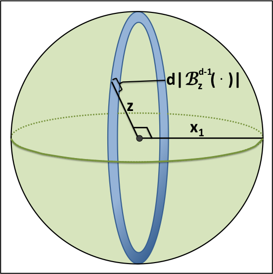
Figure 2: The differential over a lower-dimensional hyperball, illustrated for $d=3$.

Let, $\mathbb{E}[I_{n}]=\sum_{m=1}^{M}\mathbb{E}[I_{m}]$, where $I_{m}$ is the length of a single segment between two random samples in consecutive disjoint balls. Then, because all $I_{m}$ are I.I.D., $\mathbb{E}[I_{n}]=M\mathbb{E}[I_{1}]$. Then, to compute $\mathbb{E}[I_{n}]$, $\mathbb{E}[I_{1}]$ is computed. This problem is similar to the problem known as the ball-line picking problem from geometric probability Santalo (1976). The ball-line picking problem is to compute the average length of a segment lying within a d-dimensional hyperball, where the endpoints of the segment are uniformly distributed within the hyperball. The ball-line picking problem yields an analytical solution in general dimension; however, in the problem examined here, there are two disjoint hyperballs rather than a single hyperball. To the best of the authors’ knowledge, this variant of the problem has not been previously studied. Computing this value requires integration over the possible locations of the endpoints of the segment, as illustrated in Figure 3.

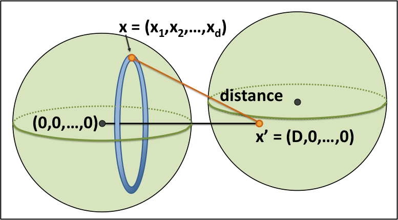
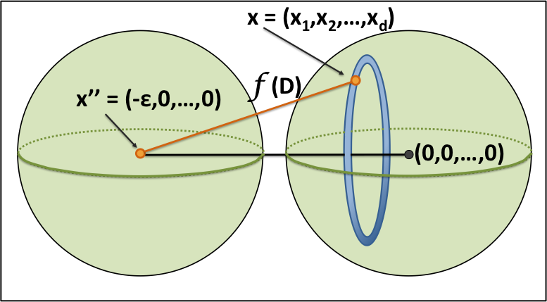
Figure 3: Illustrations in 3D of the mean calculation. (top) The first set of integrals is performed over the left hyperball, averaging the distance between points $(x_{1},x_{2},\ldots,x_{d})$ and $(D,0,\ldots,0)$. (bottom) Using the result from the first set of integrals, a second set of integrals is performed over the second hyperball, yielding the expected value.

The integration is broken into two steps, and the first integral will be for the situation depicted in Figure 3 (left). The objective is to get an expected value for the distance between points $x$ and $x^{\prime}$. Here, $x$ represents a random point within the first hyperball, while $x^{\prime}$ is some fixed point within the second hyperball which has distance $D$ from the center of the first hyperball. Without loss of generality, $x^{\prime}$ can be displaced along only the first coordinate, $x_{1}$. To get an expected value, this distance is integrated over all points within the first hyperball, and then divided by the volume of the d-dimensional hyperball. In this work, the volume of a d-dimensional hypersphere of radius $\beta_{n}$ is denoted $|\mathcal{B}_{\beta_{n}}|=V_{d}\beta_{n}^{d}$, where $V_{d}$ is a constant dependent on the dimension of the space. Taking the distance between $x=(x_{1},x_{2},\ldots,x_{d})$ and $x^{\prime}=(D,0,\ldots,0)$ to be $\sqrt{(x_{1}-D)^{2}+x_{2}^{2}+\ldots+x_{d}^{2}}$ produces the following integral:

$$A=\frac{1}{V_{d}\beta_{n}^{d}}\idotsint_{x_{1}^{2}+\ldots+x_{d}^{2}\leq\beta_{n}^{2}}\\ \sqrt{(x_{1}-D)^{2}+x_{2}^{2}+\ldots+x_{d}^{2}}\ dx_{1}\ldots dx_{d},$$

This integral will be converted from a d-dimensional integral into a double integral using substitution. First, let $z^{2}=x_{2}^{2}+\ldots+x_{d}^{2}$. This allows performing the integral over only two variables, $x_{1}$ and $z$; however, the form of the integral changes, as the differential is adapted as illustrated in Figure 2. This differential, $d|\mathcal{B}_{d-1}(z)|$, is taken over a lower dimensional hypersphere, of dimension $d-1$, as $z$ is taking the place of $d-1$ coordinates. Then:

$$A=\frac{1}{V_{d}\beta_{n}^{d}}\iint_{x_{1}^{2}+z^{2}\leq\beta_{n}^{2}}\\ \sqrt{(x_{1}-D)^{2}+z^{2}}\ d|\mathcal{B}^{d-1}_{z}(\cdot)|dx_{1}dz,$$

where $d|\mathcal{B}_{d-1}(z)|=\frac{d}{dz}V_{d-1}z^{d-1}$. Taking this derivative, $\frac{d}{dz}V_{d-1}z^{d-1}=(d-1)V_{d-1}z^{d-2}$, and substituting into $A$ yields:

$$A=\frac{(d-1)V_{d-1}}{V_{d}\beta_{n}^{d}}\iint_{x_{1}^{2}+z^{2}\leq\beta_{n}^{2}}\\ z^{d-2}\sqrt{x_{1}^{2}+D^{2}-2Dx_{1}+z^{2}}\ dx_{1}dz$$

The integral can be represented in terms of polar coordinates, where $x_{1}=r\cos\theta$, $z=r\sin\theta$, and $dx_{1}\ dz=r\ d\theta\ dr$. This gives

$$A=\frac{(d-1)V_{d-1}}{V_{d}\beta_{n}^{d}}\int_{0}^{\beta_{n}}r\int_{0}^{\pi}\\ (r\sin\theta)^{d-2}\sqrt{r^{2}+D^{2}-2Dr\cos\theta}\ d\theta dr$$

$$A=\frac{D(d-1)V_{d-1}}{V_{d}\beta_{n}^{d}}\int_{0}^{\beta_{n}}r\int_{0}^{\pi}\\ (r\sin\theta)^{d-2}\sqrt{1+\big{(}\frac{r}{D}\big{)}^{2}-2\big{(}\frac{r}{D}\big{)}\cos\theta}\ d\theta dr$$

A second-order Taylor Approximation for the square root is taken. Let $f(u)=\sqrt{1+u}$, where $u=\big{(}\frac{r}{D}\big{)}^{2}-2\big{(}\frac{r}{D}\big{)}\cos\theta$. The approximation will be taken about the point $u=0$. This is reasonable given that overall, $\beta_{n}$ is considered to be smaller than the separation between consecutive hyperballs, $\epsilon_{n}$. Take the second-order Taylor Approximation as:

$$f(u)\approx f(0)+f^{\prime}(0)\cdot u+\frac{1}{2!}f^{\prime\prime}(0)\cdot u^{2}.$$

Taking a derivative of $f$ yields $f^{\prime}(u)=\frac{1}{2}(1+u)^{-\frac{1}{2}}$ and $f^{\prime\prime}(u)=-\frac{1}{4}(1+u)^{-\frac{3}{2}}$. Then,

$$f(u)\approx\sqrt{1}+\frac{1}{2}(1)^{-\frac{1}{2}}\cdot u-\frac{1}{2}\cdot\frac{1}{4}(1)^{-\frac{3}{2}}\cdot u^{2}=1+\frac{1}{2}u-\frac{1}{8}u^{2}$$

substituting $u=\big{(}\frac{r}{D}\big{)}^{2}-2\big{(}\frac{r}{D}\big{)}\cos\theta$,

$$f(u)\approx 1+\frac{1}{2}\big{(}\big{(}\frac{r}{D}\big{)}^{2}-2\big{(}\frac{r}{D}\big{)}\cos\theta\big{)}\\ -\frac{1}{8}\big{(}\big{(}\frac{r}{D}\big{)}^{2}-2\big{(}\frac{r}{D}\big{)}\cos\theta\big{)}^{2}$$

$$f(u)\approx 1+\frac{1}{2}\big{(}\big{(}\frac{r}{D}\big{)}^{2}-2\big{(}\frac{r}{D}\big{)}\cos\theta\big{)}\\ -\frac{1}{8}\big{(}\big{(}\frac{r}{D}\big{)}^{4}-4\big{(}\frac{r}{D}\big{)}^{3}\cos\theta+4\big{(}\frac{r}{D}\big{)}^{2}\cos^{2}\theta\big{)}$$

Then, as this is a second-order approximation, the third- and fourth-order terms are considered negligible, and thus, the approximation results in:

$$f(u)\approx 1+\frac{1}{2}\big{(}\big{(}\frac{r}{D}\big{)}^{2}-2\big{(}\frac{r}{D}\big{)}\cos\theta\big{)}-\frac{1}{8}\big{(}4\big{(}\frac{r}{D}\big{)}^{2}\cos^{2}\theta\big{)}$$

Substituting the result:

$$A=\frac{D(d-1)V_{d-1}}{V_{d}\beta_{n}^{d}}\int_{0}^{\beta_{n}}r\int_{0}^{\pi}(r\sin\theta)^{d-2}\\ \Big{(}1+\frac{1}{2}\big{(}\big{(}\frac{r}{D}\big{)}^{2}+2\big{(}\frac{r}{D}\big{)}\cos\theta\big{)}-\frac{1}{8}\big{(}4\big{(}\frac{r}{D}\big{)}^{2}\cos^{2}\theta\big{)}\Big{)}\ d\theta dr$$

Simplifying this integral requires the following Lemmas:

Lemma 2 (Value of $\int_{0}^{\pi}(\sin\theta)^{d}d\theta$)

In terms of the hyperball volume constant, $V_{d}$,

$$\int_{0}^{\pi}(\sin\theta)^{d-2}d\theta=S_{d-2}=\frac{dV_{d}}{(d-1)V_{d-1}}$$

Proof

For simplicity, let $\int_{0}^{\pi}sin^{d}(\theta)\ d\theta$ be denoted as $S_{d}$. Then:

$$|\mathcal{B}_{\beta}|=V_{d}\beta^{d},$$

where $V_{d}=\frac{\pi^{\frac{d}{2}}}{\Gamma(\frac{d}{2}+1)}$ is a constant dependent on the dimension, $d$. Then, the volume can be computed as an integral of the following form:

$$V_{d}\beta^{d}=\iint_{x_{1}^{2}+\rho^{2}\leq\beta^{2}}\ dx_{1}\ d(V_{d-1}\rho^{d-1}),$$

where the second differential is over a sphere of radius $\rho$ of dimension $d-1$. Then,

$$V_{d}\beta^{d}=\iint_{x_{1}^{2}+\rho^{2}\leq\beta^{2}}(d-1)V_{d-1}\rho^{d-2}\ dx_{1}\ d\rho$$

Now, to simplify this integral, it will be converted to polar coordinates, using $x_{1}=r\ \cos\theta$, $\rho=r\ \sin\theta$, and $dx_{1}\ d\rho=r\ d\theta\ dr$. Substituting these values yields:

$$V_{d}\beta^{d}=(d-1)V_{d-1}\int_{0}^{\beta}\int_{0}^{\pi}r^{d-2}(\sin\theta)^{d-2}r\ d\theta\ dr$$

$$V_{d}\beta^{d}=(d-1)V_{d-1}\int_{0}^{\beta}r^{d-1}S_{d-2}\ d\theta\ dr$$

$$V_{d}\beta^{d}=(d-1)V_{d-1}S_{d-2}\frac{\beta^{d}}{d}\ d\theta\ dr$$

$$S_{d-2}=\frac{dV_{d}}{(d-1)V_{d-1}}\ \square$$

Lemma 3 (Recurrence relation of $\int_{0}^{\pi}(\sin\theta)^{d}d\theta$)

For $S_{d}=\int_{0}^{\pi}(\sin\theta)^{d}d\theta$, the following recurrence relation holds:

$$\int_{0}^{\pi}(\sin\theta)^{d}d\theta=S_{d}=\frac{d-1}{d}S_{d-2}$$

Proof To determine this recurrence, the following expression will be solved for $x$:

$$S_{d}=xS_{d-2}$$

Substitute the result from Lemma 2, getting:

$$x=\frac{(d+2)V_{d+2}}{(d+1)V_{d+1}}\cdot\frac{(d-1)V_{d-1}}{dV_{d}}.$$

Then, substituting the value of $V_{d}$ yields:

$$x=\frac{(d-1)(d+2)}{d(d+1)}\Big{(}\frac{\Gamma(\frac{d+2}{2})}{\Gamma(\frac{d+4}{2})}\Big{)}\Big{(}\frac{\Gamma(\frac{d+3}{2})}{\Gamma(\frac{d+1}{2})}\Big{)}$$

$$x=\frac{(d-1)(d+2)}{d(d+1)}\Big{(}\frac{2}{d+2}\Big{)}\Big{(}\frac{d+1}{2}\Big{)}$$

$$x=\frac{d-1}{d}\ \square$$

Applying these Lemmas:

$$A=\frac{D(d-1)V_{d-1}}{V_{d}\beta^{d}}\\ \int_{0}^{\beta_{n}}r\Bigg{(}\int_{0}^{\pi}(r\sin\theta)^{d-2}\Big{(}1+\frac{1}{2}\big{(}\frac{r}{D}\big{)}^{2}\Big{)}d\theta\\ +\int_{0}^{\pi}(r\sin\theta)^{d-2}(\cos\theta)d\theta\\ -\frac{1}{2}\big{(}\frac{r}{D}\big{)}^{2}\int_{0}^{\pi}(sin\theta)^{d-2}cos^{2}\theta\ d\theta\Bigg{)}dr$$

The second integral over $\theta$ will integrate to $0$, due to the presence of cosine, while the other terms leverage Lemmas 2 and 3:

$$A=\frac{D(d-1)V_{d-1}}{V_{d}\beta_{n}^{d}}\int_{0}^{\beta_{n}}\\ r^{d-1}\Bigg{(}S_{d-2}\Big{(}1+\frac{1}{2}\big{(}\frac{r}{D}\big{)}^{2}\Big{)}-\frac{1}{2}\big{(}\frac{r}{D}\big{)}^{2}\Big{(}S_{d-2}-S_{d}\Big{)}\Bigg{)}dr$$

$$A=\frac{D(d-1)V_{d-1}}{V_{d}\beta_{n}^{d}}S_{d-2}\cdot\\ \int_{0}^{\beta_{n}}r^{d-1}\Bigg{(}\Big{(}1+\frac{d-1}{2d}\big{(}\frac{r}{D}\big{)}^{2}\Big{)}\Bigg{)}dr$$

$$A=\frac{D(d-1)V_{d-1}}{V_{d}\beta_{n}^{d}}S_{d-2}\cdot\\ \int_{0}^{\beta_{n}}\Bigg{(}r^{d-1}+\frac{d-1}{2d}\Big{(}\frac{r^{d+1}}{D^{2}}\Big{)}\Bigg{)}dr$$

$$A=\frac{D(d-1)V_{d-1}}{V_{d}\beta_{n}^{d}}\frac{dV_{d}}{(d-1)V_{d-1}}\cdot\\ \Bigg{(}\frac{\beta_{n}^{d}}{d}+\frac{d-1}{2d}\Big{(}\frac{\beta_{n}^{d+2}}{(d+2)D^{2}}\Big{)}\Bigg{)}\\ =D+\frac{(d-1)\beta_{n}^{2}}{2(d+2)D}$$

This is only an intermediate result, however, and it must be integrated over once again to consider all possible placements of the point $x^{\prime}$ in the second hyperball, as illustrated in Figure 3(right). In order to do so, write $D$ in terms of $\epsilon$ by taking the distance between $x=(x_{1},x_{2},\ldots,x_{d})$ and $x^{\prime\prime}=(-\epsilon_{n},0,\ldots,0)$. Then, $D=\sqrt{(x_{1}+\epsilon)^{2}+x_{2}^{2}+\ldots+x_{d}^{2}}$, and $\mathbb{E}[I_{1}]$ is computed as:

$$\mathbb{E}[I_{1}]=\frac{1}{V_{d}\beta_{n}^{d}}\idotsint_{x_{1}^{2}+\ldots+x_{d}^{2}\leq\beta_{n}^{2}}D\\ +\frac{(d-1)\beta_{n}^{2}}{2(d+2)D}\ dx_{1}\ldots dx_{d},$$

Steps similar to what was just taken to derive the intermediate result are used to compute this integral. As a matter of simplicity, note that the second term inside the integral is already a second-order term, which means taking the integral will result in higher-order terms. Since $D=\sqrt{(x_{1}+\epsilon_{n})^{2}+x_{2}^{2}+\ldots+x_{d}^{2}}$, the second term will take only the constant term of the Taylor Approximation for $D$. Then, taking $z^{2}=x_{2}^{2}+\ldots+x_{d}^{2}$:

$$\mathbb{E}[I_{m}]=\frac{1}{V_{d}\beta_{n}^{d}}\idotsint_{x_{1}^{2}+\ldots+x_{d}^{2}\leq\beta_{n}^{2}}\\ \sqrt{(x_{1}+\epsilon_{n})^{2}+x_{2}^{2}+\ldots+x_{d}^{2}}\ \\ +\frac{(d-1)\beta_{n}^{2}}{2(d+2)\sqrt{(x_{1}+\epsilon_{n})^{2}+x_{2}^{2}+\ldots+x_{d}^{2}}}\ dx_{1}\ldots dx_{d}$$

$$\mathbb{E}[I_{m}]=\frac{1}{V_{d}\beta_{n}^{d}}\iint_{x_{1}^{2}+z^{2}\leq\beta_{n}^{2}}\sqrt{(x_{1}+\epsilon_{n})^{2}+z^{2}}\\ +\frac{(d-1)\beta_{n}^{2}}{2(d+2)\sqrt{(x_{1}+\epsilon_{n})^{2}+z^{2}}}\ dx_{1}\ dz$$

Again, perform a polar coordinate transformation so as to take the integral:

$$\mathbb{E}[I_{m}]=\frac{1}{V_{d}\beta_{n}^{d}}\int_{0}^{\beta_{n}}r\int_{0}^{\pi}\Big{(}\sqrt{r^{2}+\epsilon_{n}^{2}-2\epsilon_{n}r\cos\theta}\\ +\frac{(d-1)\beta_{n}^{2}}{2(d+2)\sqrt{r^{2}+\epsilon_{n}^{2}-2\epsilon_{n}r\cos\theta}}\Big{)}d|\mathcal{B}^{d-1}_{r\sin\theta}(\cdot)|\ d\theta\ dr$$

$$\mathbb{E}[I_{m}]=\frac{(d-1)V_{d-1}}{V_{d}\beta_{n}^{d}}\int_{0}^{\beta_{n}}r\int_{0}^{\pi}(r\ \sin\theta)^{d-2}\\ \Big{(}\sqrt{r^{2}+\epsilon_{n}^{2}-2\epsilon_{n}r\cos\theta}\\ +\frac{(d-1)\beta_{n}^{2}}{2(d+2)\sqrt{r^{2}+\epsilon_{n}^{2}-2\epsilon_{n}r\cos\theta}}\Big{)}\ d\theta\ dr$$

Now, to compute this integral, a Taylor Approximation will be taken. Again, recall that because the second term in the integral is second order, a $0^{th}$-order approximation is taken for that term:

$$\mathbb{E}[I_{m}]\approx\frac{(d-1)V_{d-1}}{V_{d}\beta_{n}^{d}}\int_{0}^{\beta_{n}}r\int_{0}^{\pi}(r\ \sin\theta)^{d-2}\\ \Big{(}\epsilon_{n}\Big{(}1+\frac{1}{2}\big{(}\big{(}\frac{r}{\epsilon_{n}}\big{)}^{2}+2\big{(}\frac{r}{\epsilon_{n}}\big{)}\cos\theta\big{)}-\frac{1}{8}\big{(}4\big{(}\frac{r}{\epsilon_{n}}\big{)}^{2}\cos^{2}\theta\big{)}\Big{)}\\ +\frac{(d-1)\beta_{n}^{2}}{2(d+2)\epsilon_{n}}\Big{)}\ d\theta\ dr$$

Then, performing steps similar to above, rewrite in terms of $S_{d-2}$, as well as splitting the last term into a separate integral:

$$\mathbb{E}[I_{m}]\approx\frac{\epsilon_{n}(d-1)V_{d-1}}{V_{d}\beta_{n}^{d}}\int_{0}^{\beta_{n}}r^{d-1}\int_{0}^{\pi}\Big{(}(\sin\theta)^{d-2}\\ +\frac{r^{2}}{2\epsilon_{n}^{2}}(\sin\theta)^{d}\Big{)}\ d\theta\ dr+\frac{(d-1)V_{d-1}}{V_{d}\beta_{n}^{d}}\cdot\\ \int_{0}^{\beta_{n}}r^{d-1}\int_{0}^{\pi}(\sin\theta)^{d-2}\frac{(d-1)\beta_{n}^{2}}{2(d+2)\epsilon_{n}}\ d\theta\ dr$$

$$\mathbb{E}[I_{m}]\approx\frac{\epsilon_{n}(d-1)V_{d-1}}{V_{d}\beta_{n}^{d}}S_{d-2}\int_{0}^{\beta_{n}}r^{d-1}\Big{(}1\\ +\frac{(d-1)r^{2}}{2d\epsilon_{n}^{2}}\Big{)}\ dr+\frac{\epsilon_{n}(d-1)V_{d-1}}{V_{d}\beta_{n}^{d}}S_{d-2}\\ \int_{0}^{\beta_{n}}r^{d-1}\frac{(d-1)\beta_{n}^{2}}{2(d+2)\epsilon_{n}^{2}}\ dr$$

$$\mathbb{E}[I_{m}]\approx\frac{\epsilon_{n}(d-1)V_{d-1}}{V_{d}\beta_{n}^{d}}S_{d-2}\Big{(}\frac{\beta_{n}^{d}}{d}+\frac{(d-1)\beta_{n}^{d+2}}{2d(d+2)\epsilon_{n}^{2}}\Big{)}\\ +\frac{\epsilon_{n}(d-1)V_{d-1}}{V_{d}\beta_{n}^{d}}S_{d-2}\Big{(}\frac{(d-1)\beta_{n}^{d+2}}{2d(d+2)\epsilon_{n}^{2}}\Big{)}$$

$$\mathbb{E}[I_{m}]\approx\frac{\epsilon_{n}(d-1)V_{d-1}}{V_{d}\beta_{n}^{d}}\frac{dV_{d-1}}{(d-1)V_{d-1}}\cdot\\ \Big{(}\frac{\beta_{n}^{d}}{d}+\frac{(d-1)\beta_{n}^{d+2}}{2d(d+2)\epsilon_{n}^{2}}+\frac{(d-1)\beta_{n}^{d+2}}{2d(d+2)\epsilon_{n}^{2}}\Big{)}$$

$$\mathbb{E}[I_{m}]\approx\epsilon_{n}+\frac{(d-1)\beta_{n}^{2}}{(d+2)\epsilon_{n}}$$

Now, using this result for the expected value of a single segment, $I_{m}$, the expected value of the entire path consisting of $M$ such segments is:

$$\mathbb{E}[I_{n}]\approx M\Big{(}\epsilon_{n}+\frac{(d-1)\beta_{n}^{2}}{(d+2)\epsilon_{n}}\Big{)}$$

Lemma 4 (Expected value of $I_{n}$)

For a path constructed over the set of $M_{n}+1$ hyperballs having radius $\beta_{n}$ has expected length:

$$\mathbb{E}[I_{n}]\approx M_{n}\Big{(}\epsilon_{n}+\frac{(d-1)\beta_{n}^{2}}{(d+2)\epsilon_{n}}\Big{)}$$

Euclidean	$\lambda_{n}=0.5$	$\lambda_{n}=0.125$
dimension	$100\cdot\frac{|\mathbb{E}[I_{n}]-I_{n}|}{I_{n}}$	$100\cdot\frac{|\mathbb{E}[I_{n}]-I_{n}|}{I_{n}}$
2	0.1730%	0.0050%
3	0.0473%	0.0205%
10	0.9413%	0.0128%
100	1.9147%	0.0129%

Figure 4: Simulation comparison for $\mathbb{E}[I_{n}]$, using 120,000 data points for each entry, for differing $\lambda_{n}=\frac{\beta_{n}}{\epsilon_{n}}$

To verify that the approximation for the expected value is tight, Monte Carlo experiments were run and compared against the drawn approximate value. The relative error of the approximation to the simulated values are shown in Figure 4. The computed approximation deviates more from experimental data as dimensionality increases, but holds quite well, especially for small values of $\lambda_{n}=\frac{\beta_{n}}{\epsilon_{n}}$.

3.6 Computation of the Variance of $I_{n}$ in $\mathbb{R}^{d}$

To compute the $Var(I_{n})$, leverage the definition of the variance of a random variable, i.e. $Var(X)=\mathbb{E}[X^{2}]-(\mathbb{E}[X])^{2}$:

$$Var\big{(}\sum_{m=1}^{M}I_{m}\big{)}=\mathbb{E}[\sum_{m=1}^{M}I_{m}^{2}]-\big{(}\mathbb{E}[\sum_{m=1}^{M}I_{m}]\big{)}^{2}\\ =\sum_{m=1}^{M}\sum_{k=1}^{M}\mathbb{E}[I_{m}I_{k}]-\big{(}\mathbb{E}[\sum_{m=1}^{M}I_{m}]\big{)}^{2}$$

The second term can be simplified due to the linearity of expectation, which allows the double sum to be simplified:

$$Var\big{(}\sum_{m=1}^{M}I_{m}\big{)}=\sum_{m=1}^{M}\sum_{k=1}^{M}\mathbb{E}[I_{m}I_{k}]-M^{2}\big{(}\mathbb{E}[I_{m}]\big{)}^{2}$$

Then, the first term consists of the expected value of the product of all $M^{2}$ pairs of segments along a path. There are variance terms for each segment with itself, i.e. $\mathbb{E}[I_{m}^{2}]$, of which there are $M$. Additionally, pairs of segments which share an endpoint have a dependence. Only consecutive pairs have such a dependence, and each segment depends on two neighbors, or a total of $2M$ dependencies, except that the start and end segments only have a single neighbor, which yields a total of $2M-2$ such dependencies. Then, all of the other segments must be independent. Then, expand the double sum as:

$$\sum_{m=1}^{M}\sum_{k=1}^{M}\mathbb{E}[I_{m}I_{k}]=M\mathbb{E}[I_{m}^{2}]+(2M-2)\mathbb{E}[I_{m}I_{m+1}]\\ +(M^{2}-M-(2M-2))\mathbb{E}[I_{m}I_{m+2}]$$

where $I_{m}$ and $I_{m+2}$ are independent, and $I_{m}$ and $I_{m+1}$ are dependent consecutive segments. Due to this independence, and substituting $m=1$ yields:

$$Var\big{(}\sum_{m=1}^{M}I_{m}\big{)}=M\mathbb{E}[I_{1}^{2}]+(2M-2)\mathbb{E}[I_{1}I_{2}]\\ +(M^{2}-M-(2M-2))\mathbb{E}[I_{1}]\mathbb{E}[I_{1}]-M^{2}\big{(}\mathbb{E}[I_{1}]\big{)}^{2}$$

This results in a final variance term:

$$Var\big{(}\sum_{m=1}^{M}I_{m}\big{)}=M\mathbb{E}[I_{1}^{2}]\\ +(2M-2)\mathbb{E}[I_{1}I_{2}]+(2-3M)\big{(}\mathbb{E}[I_{1}]\big{)}^{2}$$

From the previous section, the value for $(\mathbb{E}[I_{1}])^{2}$ is available; however, both $\mathbb{E}[I_{1}^{2}]$ and $\mathbb{E}[I_{1}I_{2}]$ must be computed.

3.6.1 Approximation of $\mathbb{E}[I_{1}^{2}]$ in $\mathbb{R}^{d}$.

The derivation of $\mathbb{E}[I_{1}^{2}]$ follows the same general steps as the computation of $\mathbb{E}[I_{1}]$; however, the form of the integral is simpler in this case. The integral over one of the two balls is of the form:

$$A=\frac{1}{V_{d}{\beta_{n}}^{d}}\idotsint_{x_{1}^{2}+\ldots+x_{d}^{2}\leq{\beta_{n}}^{2}}\\ \Big{(}\sqrt{(D-x_{1})^{2}+x_{2}^{2}+\ldots+x_{d}^{2}}\Big{)}^{2}dx_{1}\dots dx_{d},$$

$A$ represents an intermediate result. Then, take $z^{2}=x_{2}^{2}+\ldots+x_{d}^{2}$. Substituting these into the above integral yields:

$$\frac{1}{V_{d}{\beta_{n}}^{d}}\iint_{x_{1}^{2}+z^{2}\leq{\beta_{n}}^{2}}\big{(}(D-x_{1})^{2}+z^{2}\ d|\mathcal{B}^{d-1}_{z}(\cdot)|\big{)}\ dx_{1}dz$$

$$=\frac{1}{V_{d}{\beta_{n}}^{d}}\iint_{x_{1}^{2}+z^{2}\leq{\beta_{n}}^{2}}\\ V_{d-1}(d-1)z^{d-2}\big{(}(D-x_{1})^{2}+z^{2}\big{)}\ dx_{1}dz$$

Then, to compute this integral, perform the integration over polar coordinates:

$$\frac{V_{d-1}(d-1)}{V_{d}{\beta_{n}}^{d}}\int_{0}^{\beta_{n}}r\int_{0}^{\pi}(r\ \sin\theta)^{d-2}\\ \big{(}(D-(r\ \cos\theta))^{2}+(r\ \sin\theta)^{2}\big{)}\ d\theta\ dr$$

$$=\frac{V_{d-1}(d-1)}{V_{d}{\beta_{n}}^{d}}\int_{0}^{\beta_{n}}r^{d-1}\int_{0}^{\pi}(\sin\theta)^{d-2}\\ \big{(}D^{2}+r^{2}-2Dr\cos\theta\big{)}\ d\theta\ dr$$

Then, applying Lemmas 2 and 3:

$$\frac{V_{d-1}(d-1)}{V_{d}{\beta_{n}}^{d}}\int_{0}^{\beta_{n}}r^{d-1}\big{(}D^{2}+r^{2}\big{)}S_{d-2}\ d\theta\ dr$$

$$=\frac{V_{d-1}(d-1)S_{d-2}}{V_{d}{\beta_{n}}^{d}}\big{(}D^{2}\frac{{\beta_{n}}^{d}}{d}+\frac{d{\beta_{n}}^{d+2}}{d(d+2)}\big{)}\ d\theta\ dr$$

$$A=D^{2}+\frac{d}{d+2}{\beta_{n}}^{2}$$

Now, this intermediate result is used to compute the final value of $\mathbb{E}[I_{1}^{2}]$. Begin again by integrating over this value:

$$\mathbb{E}[I_{1}^{2}]=\frac{1}{V_{d}{\beta_{n}}^{d}}\idotsint_{x_{1}^{2}+\ldots+x_{d}^{2}\leq{\beta_{n}}^{2}}D^{2}\\ +\frac{d}{d+2}{\beta_{n}}^{2}dx_{1}\dots dx_{d},$$

where now $D$ is written in terms of $\epsilon_{n}$ as $D=\sqrt{(x_{1}+\epsilon_{n})^{2}+x_{2}^{2}+\ldots+x_{d}^{2}}$. Again, take $z^{2}=x_{2}^{2}+\ldots+x_{d}^{2}$ and substitute in to get:

$$\frac{1}{V_{d}{\beta_{n}}^{d}}\iint_{x_{1}^{2}+z^{2}\leq{\beta_{n}}^{2}}\\ \big{(}((x_{1}+\epsilon_{n})^{2}+z^{2})+\frac{d}{d+2}{\beta_{n}}^{2}\big{)}d|\mathcal{B}^{d-1}_{z}(\cdot)|\ dx_{1}\ dz$$

$$=\frac{(d-1)V_{d-1}}{V_{d}{\beta_{n}}^{d}}\iint_{x_{1}^{2}+z^{2}\leq{\beta_{n}}^{2}}\\ \big{(}(r^{2}+\epsilon_{n}^{2}+2x_{1}\epsilon_{n})+\frac{d}{d+2}{\beta_{n}}^{2}\big{)}z^{d-2}\ dx_{1}\ dz$$

Rewrite in polar coordinates and splitting the integral:

$$\frac{(d-1)V_{d-1}}{V_{d}{\beta_{n}}^{d}}\Bigg{(}\int_{0}^{\beta_{n}}r\int_{0}^{\pi}r^{d}(\sin\theta)^{d-2}\\ +(r\sin\theta)^{d-2}\epsilon_{n}^{2}+2\epsilon_{n}r\cos\theta d\theta\ dr\\ +\frac{d}{d+2}{\beta_{n}}^{2}\int_{0}^{\beta_{n}}r\int_{0}^{\pi}(r\sin\theta)^{d-2}\ d\theta\ dr\Bigg{)}$$

$$=\frac{(d-1)V_{d-1}}{V_{d}{\beta_{n}}^{d}}\Bigg{(}\int_{0}^{\beta_{n}}r\big{(}S_{d-2}(r^{d}+\epsilon_{n}^{2}r^{d-2})\big{)}dr\\ +\frac{d}{d+2}{\beta_{n}}^{2}\int_{0}^{\beta_{n}}r^{d-1}S_{d-2}dr\Bigg{)}$$

$$=\frac{(d-1)V_{d-1}}{V_{d}{\beta_{n}}^{d}}S_{d-2}\Bigg{(}\frac{{\beta_{n}}^{d+2}}{d+2}+\frac{\epsilon_{n}^{2}{\beta_{n}}^{d}}{d}+\frac{d{\beta_{n}}^{2}}{d+2}+\frac{{\beta_{n}}^{d}}{d}\Bigg{)}$$

$$\mathbb{E}[I_{1}^{2}]=\epsilon_{n}^{2}+\frac{2d}{d+2}{\beta_{n}}^{2}$$

Lemma 5 (Expected value of $I_{1}^{2}$)

For two consecutive hyperballs, the expected squared distance between random points in those spheres is

$$\mathbb{E}[I_{1}^{2}]=\epsilon_{n}^{2}+\frac{2d}{d+2}\beta_{n}^{2}$$

3.6.2 Approximation of $\mathbb{E}[I_{1}I_{2}]$ in $\mathbb{R}^{d}$.

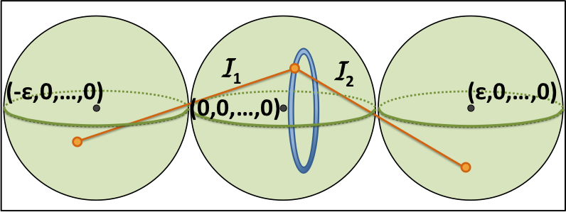
Figure 5: To compute $\mathbb{E}[I_{1}I_{2}]$, integration is performed over the common point determining $I_{1}$ and $I_{2}$.

To compute $\mathbb{E}[I_{1}I_{2}]$, a key observation is made. First, to retrieve this value, the reasoning must consider three consecutive hyperballs, where the distance between the samples of the first two balls, $I_{1}$, and the distance between the samples of the second and third balls, $I_{2}$, depend on each other through their common endpoint in the second ball. Consider, however, that if this second point is fixed, then the values of $I_{1}$ and $I_{2}$ become independent. Using this fact, and the intermediate result of the mean calculation, begin by simply multiplying these two means to get the intermediate result:

$$A=(D_{1}+\frac{C_{d}\beta_{n}^{2}}{2D_{1}})(D_{2}+\frac{C_{d}\beta_{n}^{2}}{2D_{2}})$$

$$A=D_{1}D_{2}+\frac{C_{d}\beta_{n}^{2}}{2}\Big{(}\frac{D_{1}}{D_{2}}+\frac{D_{2}}{D_{1}}\Big{)}$$

where the fourth-order term involving $\beta_{n}^{4}$ is negligible.

Now, to reintroduce the dependence of $I_{1}$ and $I_{2}$, integrate over the second ball. For technical reasons, it is assumed that the centers of the three hyperballs are collinear. Then, the integral to solve is the following:

$$\mathbb{E}[I_{1}I_{2}]=\frac{1}{V_{d}{\beta_{n}}^{d}}\idotsint_{x_{1}^{2}+\ldots+x_{d}^{2}\leq{\beta_{n}}^{2}}D_{1}D_{2}\\ +\frac{(d-1){\beta_{n}}^{2}}{2(d+2)}\Big{(}\frac{D_{2}}{D_{1}}+\frac{D_{1}}{D_{2}}\Big{)}\ dx_{1}\ldots dx_{d}$$

Where $D_{1}$ and $D_{2}$ are expressed in relative to the center of the middle hyperball as $D_{1}=\sqrt{(x_{1}-\epsilon)^{2}+x_{2}^{2}+\ldots+x_{d}^{2}}$ and $D_{2}=\sqrt{(x_{1}+\epsilon)^{2}+x_{2}^{2}+\ldots+x_{d}^{2}}$. Again, taking $z^{2}=x_{2}^{2}+\ldots x_{d}^{2}$ and then, because the second term is already second-order, take a $0^{th}$-order approximation over only that term:

$$\mathbb{E}[I_{1}I_{2}]\approx\frac{1}{V_{d}{\beta_{n}}^{d}}\iint_{x_{1}^{2}+z^{2}\leq{\beta_{n}}^{2}}\\ \Bigg{(}\sqrt{(x_{1}-\epsilon_{n})^{2}+z^{2}}\sqrt{(x_{1}+\epsilon_{n})^{2}+z^{2}}\\ +\frac{(d-1){\beta_{n}}^{2}}{2(d+2)}\Big{(}\frac{\epsilon_{n}}{\epsilon_{n}}+\frac{\epsilon_{n}}{\epsilon_{n}}\Big{)}\Bigg{)}d|\mathcal{B}^{d-1}_{z}(\cdot)|\ dx_{1}dz$$

Again, convert this integral into polar coordinates:

$$\mathbb{E}[I_{1}I_{2}]\approx\frac{(d-1)V_{d-1}}{V_{d}{\beta_{n}}^{d}}\int_{0}^{\beta_{n}}r\int_{0}^{\pi}(r\ \sin\theta)^{d-2}\\ \Bigg{(}\sqrt{r^{2}+\epsilon_{n}^{2}-2\epsilon_{n}r\cos\theta}\sqrt{r^{2}+\epsilon_{n}^{2}+2\epsilon_{n}r\cos\theta}\\ +\frac{(d-1){\beta_{n}}^{2}}{(d+2)}\Bigg{)}\ d\theta\ dr$$

$$\mathbb{E}[I_{1}I_{2}]\approx\frac{\epsilon_{n}^{2}(d-1)V_{d-1}}{V_{d}{\beta_{n}}^{d}}\int_{0}^{\beta_{n}}r^{d-1}\int_{0}^{\pi}(\sin\theta)^{d-2}\\ \Bigg{(}\sqrt{1+2\Big{(}\frac{r}{\epsilon_{n}}\Big{)}^{2}-4\Big{(}\frac{r}{\epsilon_{n}}\Big{)}^{2}\cos^{2}\theta}+\frac{(d-1){\beta_{n}}^{2}}{(d+2)}\Bigg{)}\ d\theta\ dr$$

Then, as the square root is prohibitive to integrate directly, a second-order Taylor approximation is employed:

$$\mathbb{E}[I_{1}I_{2}]\approx\frac{\epsilon_{n}^{2}(d-1)V_{d-1}}{V_{d}{\beta_{n}}^{d}}\int_{0}^{\beta_{n}}r^{d-1}\int_{0}^{\pi}(\sin\theta)^{d-2}\\ \Bigg{(}1+\Big{(}\frac{r}{\epsilon_{n}}\Big{)}^{2}-2\Big{(}\frac{r}{\epsilon_{n}}\Big{)}^{2}\cos^{2}\theta+\frac{(d-1){\beta_{n}}^{2}}{(d+2)}\Bigg{)}\ d\theta\ dr$$

$$\mathbb{E}[I_{1}I_{2}]\approx\frac{\epsilon_{n}^{2}(d-1)V_{d-1}}{V_{d}{\beta_{n}}^{d}}\int_{0}^{\beta_{n}}r^{d-1}\int_{0}^{\pi}(\sin\theta)^{d-2}\\ \Bigg{(}1-\Big{(}\frac{r}{\epsilon_{n}}\Big{)}^{2}+2\Big{(}\frac{r}{\epsilon_{n}}\Big{)}^{2}\sin^{2}\theta+\frac{(d-1){\beta_{n}}^{2}}{(d+2)}\Bigg{)}\ d\theta\ dr$$

$$\mathbb{E}[I_{1}I_{2}]\approx\frac{\epsilon_{n}^{2}(d-1)V_{d-1}}{V_{d}{\beta_{n}}^{d}}S_{d-2}\int_{0}^{\beta_{n}}r^{d-1}\\ \Bigg{(}1-\Big{(}\frac{r}{\epsilon_{n}}\Big{)}^{2}+\frac{2(d-1)}{d}\Big{(}\frac{r}{\epsilon_{n}}\Big{)}^{2}+\frac{(d-1){\beta_{n}}^{2}}{(d+2)}\Bigg{)}\ dr$$

$$\mathbb{E}[I_{1}I_{2}]\approx\frac{d\epsilon_{n}^{2}}{{\beta_{n}}^{d}}\Bigg{(}\frac{{\beta_{n}}^{d}}{d}-\frac{{\beta_{n}}^{d+2}}{\epsilon_{n}^{2}(d+2)}\\ +\frac{(2d-2){\beta_{n}}^{d+2}}{d\epsilon_{n}^{2}(d+2)}+\frac{(d-1){\beta_{n}}^{2}}{(d+2)}\Bigg{)}$$

$$\mathbb{E}[I_{1}I_{2}]\approx\epsilon_{n}^{2}+\Big{(}\frac{2d-3}{d+2}\Big{)}{\beta_{n}}^{2}$$

Lemma 6 (Expected value of $I_{1}I_{2}$ in $\mathbb{R}^{d}$)

For three consecutive hyperballs, the expected value of of the product of the lengths of the segments connecting random samples inside those balls is

$$\mathbb{E}[I_{1}I_{2}]\approx\epsilon_{n}^{2}+\Big{(}\frac{2d-3}{d+2}\Big{)}\beta_{n}^{2}$$

3.6.3 Combining the Lemmas to compute $Var(\sum_{m=1}^{M}I_{m})$ in $\mathbb{R}^{d}$

Computing the final variance now simply requires plugging in the values from Lemmas 4 to 6. Start with the expression computed at the beginning of this section:

$$Var\big{(}\sum_{m=1}^{M}I_{m}\big{)}=M\mathbb{E}[I_{1}^{2}]\\ +(2M-2)\mathbb{E}[I_{1}I_{2}]+(2-3M)\big{(}\mathbb{E}[I_{1}]\big{)}^{2},$$

and substitute the computed values:

$$Var\big{(}\sum_{m=1}^{M}I_{m}\big{)}\approx M\Big{(}\epsilon_{n}^{2}+\frac{2d}{d+2}\beta^{2}\Big{)}\\ +(2M-2)\Big{(}\epsilon_{n}^{2}+\frac{2d-3}{d+2}\beta^{2}\Big{)}\\ +(2-3M)\Big{(}\epsilon_{n}+\frac{(d-1)\beta^{2}}{(d+2)\epsilon_{n}}\Big{)}^{2}$$

$$Var\big{(}\sum_{m=1}^{M}I_{m}\big{)}\approx M\epsilon_{n}^{2}+\frac{2Md}{d+2}\beta^{2}+2M\epsilon_{n}^{2}\\ +\frac{4Md-6M}{d+2}\beta^{2}-2\epsilon_{n}^{2}-\frac{4d-6}{d+2}\beta^{2}+2\epsilon_{n}^{2}\\ +\frac{4d-4}{d+2}{\beta_{n}}^{2}-3M\epsilon_{n}^{2}-\frac{6Md-6M}{d+2}{\beta_{n}}^{2}$$

$$Var\big{(}\sum_{m=1}^{M}I_{m}\big{)}\approx\frac{{\beta_{n}}^{2}}{d+2}\Big{(}2Md+4Md-6M-4d\\ +6+4d-4-6Md+6\Big{)}$$

$$Var\big{(}\sum_{m=1}^{M}I_{m}\big{)}=Var(I_{n})\approx\frac{2{\beta_{n}}^{2}}{d+2}$$

Lemma 7 (Variance of $I_{n}$)

$$Var(I_{n})\approx\frac{2\beta_{n}^{2}}{d+2}$$

Euclidean	$\lambda_{n}=0.5$	$\lambda_{n}=0.125$
dimension	$\%$ error	$\%$ error
2	6.0245%	0.5739%
3	9.7691%	1.0655%
10	19.0989%	2.1429%
100	23.7279%	2.8191%

Figure 6: Simulation comparison for $Var(I_{n})$, using 120,000 data points for each entry, where the error is $100\cdot\frac{|Var(I_{n})-Var^{MC}|}{Var^{MC}}$.

Monte Carlo simulations are used to verify that the drawn approximation of the variance characterizes the variance properly. The relative error of the variance is higher than for the mean; however, for small values of $\lambda$, the approximation becomes tighter. Interestingly, up to a second-order Taylor Approximation, the variance relies only on $\beta_{n}$, and not on the length of the optimal path, $I_{\epsilon_{n}}^{*}$.

3.7 Finalizing the ${\tt PNO}$ guarantee of ${\tt PRM}^{*}$

Now that the mean and variance of $I_{n}$ has been approximated, the derivation of the bound can continue. Recall that in Section 3.4, the bound was manipulated into the following form:

$$\mathbb{P}\big{(}|I_{n}-I_{\epsilon_{n}}^{*}|\geq\delta\cdot I_{\epsilon_{n}}^{*}\ |\ \Omega_{n}^{\beta}\big{)}\\ =2\mathbb{P}\big{(}y>(\delta+1)I_{\epsilon_{n}}^{*}-\mathbb{E}(I_{n})\ |\ \Omega_{n}^{\beta}\big{)}$$

Now, substituting the computed values into this expression:

$$2\mathbb{P}\big{(}y>(\delta+1)M_{n}\epsilon_{n}-M_{n}\big{(}\epsilon_{n}+\frac{(d-1)\beta_{n}^{2}}{(d+2)\epsilon_{n}}\big{)}\ |\ \Omega_{n}^{\beta}\big{)}$$

$$=2\mathbb{P}\big{(}y>M_{n}\epsilon_{n}\big{(}\delta-\frac{(d-1)\beta_{n}^{2}}{(d+2)\epsilon_{n}^{2}}\big{)}\ |\ \Omega_{n}^{\beta}\big{)}$$

Recall that the inequality leveraged is Chebyshev’s Inequality:

$$\mathbb{P}(|X-\mathbb{E}[X]|\geq a)\leq\frac{Var(X)}{a^{2}}$$

then application of this inequality yields:

$$\mathbb{P}\big{(}|I_{n}-I_{\epsilon_{n}}^{*}|>\delta\cdot I_{\epsilon_{n}}^{*}\ |\ \Omega_{n}^{\beta}\big{)}\leq\chi,\\ \text{where }\chi=\frac{\frac{4\lambda_{n}^{2}\epsilon_{n}^{2}}{d+2}}{{I_{\epsilon_{n}}^{*}}^{2}\big{(}\delta-\frac{(d-1)}{(d+2)}\lambda_{n}^{2}\big{)}^{2}},$$

where $\lambda_{n}=\frac{\beta_{n}}{\epsilon_{n}}$. Then, the unconditional probability can be bounded as:

$$\mathbb{P}\big{(}|I_{n}-I_{\epsilon_{n}}^{*}|\geq\delta\cdot I_{\epsilon_{n}}^{*}\big{)}\leq\chi\mathbb{P}(\Omega_{n}^{\beta})+(1-\mathbb{P}(\Omega_{n}^{\beta}))$$

$$\mathbb{P}\big{(}|I_{n}-I_{\epsilon_{n}}^{*}|\geq\delta\cdot I_{\epsilon_{n}}^{*}\big{)}\leq 1+\mathbb{P}\big{(}\Omega_{n}^{\beta}\big{)}(\chi-1)$$

This leads to the following Theorem:

Thm. 1 (Probabilistic Near-Optimality of ${\tt PRM}^{*}$)

For finite iterations $n$, ${\tt PRM}^{*}$ is probabilistically near-optimal, building a graph containing a path of length $I_{n}$ such that

$$\mathbb{P}\big{(}|I_{n}-I_{\epsilon_{n}}^{*}|\geq\delta\cdot I_{\epsilon_{n}}^{*}\big{)}\leq 1+\mathbb{P}\big{(}\Omega_{n}^{\beta}\big{)}(\chi-1)$$

This bound involves several variables, many of which are known. For instance, the path-length bound $\delta$ is required as input. The parameter $M_{n}$ is a function of the length of the optimal path $I_{\epsilon_{n}}^{*}$ and $\epsilon_{n}$. The length of the optimal path is not known in general, so a pessimistic estimate is required when leveraging this guarantee. To get such an estimate, if ${\tt PRM}^{*}$ has returned a solution, its length can be used as an estimate for $I_{\epsilon_{n}}^{*}$. This bound also depends on the radius of the hyperballs, $\beta_{n}$, and on the number of samples generated in $\mathcal{C}_{\text{free}}$, $n$.

3.8 Extending ${\tt PNO}$ to roadmap spanners.

The roadmaps created with asymptotically optimal planners can be prohibitively large for practical use. Roadmap spanners have been proposed as practical methods for returning high-quality solutions while reducing memory requirements Marble and Bekris (2013). These methods provide the property of asymptotic near-optimality, i.e. as the algorithm runs to infinity, the probability that they return a path no more than $t$ times the optimal converges to $1$. The Sequential Roadmap Spanner (${\tt SRS}$) method performs a roadmap spanner technique over the resulting roadmap of ${\tt PRM}^{*}$, ensuring that paths generated by ${\tt SRS}$ are no more than $t$ times longer than corresponding ${\tt PRM}^{*}$ paths. This parameter is known as the stretch of the spanner, and is taken as input to the method.

This method was extended to work in an incremental fashion as well, known as the Incremental Roadmap Spanner (${\tt IRS}$) method. Both ${\tt SRS}$ and ${\tt IRS}$ ensure as an invariant that paths returned do not violate the stretch $t$, but consider all of the same samples and connections that ${\tt PRM}^{*}$ would. This leads to the following Lemma:

Corr. 1 (Probabilistic Near-Optimality of ${\tt SRS}$ and ${\tt IRS}$)

For finite iterations $n$ and input stretch $t$, ${\tt SRS}$ and ${\tt IRS}$ are probabilistically near optimal, constructing a path of length $I_{span}$ such that

$$\mathbb{P}\big{(}|I_{span}-t\cdot I_{\epsilon_{n}}^{*}|\geq\delta\cdot t\cdot I_{\epsilon_{n}}^{*}\big{)}\leq 1+\mathbb{P}\big{(}\Omega_{n}^{\beta}\big{)}(\chi-1)$$

4 Using ${\tt PNO}$ properties in practice

The derived probabilistic near-optimality guarantee of ${\tt PRM}^{*}$ can be leveraged in several useful ways in practice. This section shows how it can be used to estimate the length of the optimal path solving a query in the same homotopic class as the current solution during runtime. It can also provide an automated stopping criterion which probabilistically guarantees high-quality paths as well.

4.1 Online Prediction of $I_{\epsilon_{n}}^{*}$

The guarantee can be leveraged to make a prediction of the length of the optimal path which answers a query during online execution of the algorithm within a confidence bound $\mathbb{P}_{success}=\mathbb{P}(|I_{n}-I_{\epsilon_{n}}^{*}|<\delta\cdot I_{\epsilon_{n}}^{*})$. A practical method for creating the estimate of $I_{\epsilon_{n}}^{*}$ would be to consider $M_{n}$ for the given $\epsilon_{n}$ and of the current returned path length from the algorithm, $I_{n}$, and set $I_{\epsilon_{n}}^{*}=\frac{I_{n}}{(\delta+1)}$. Recall that:

$$\mathbb{P}\big{(}|I_{n}-I_{\epsilon_{n}}^{*}|\geq\delta\cdot I_{\epsilon_{n}}^{*}\big{)}\leq 1+\mathbb{P}\big{(}\Omega_{n}^{\beta}\big{)}(\chi-1)$$

Furthermore, it was shown that:

$$\mathbb{P}\big{(}|I_{n}-I_{\epsilon_{n}}^{*}|\geq\delta\cdot I_{\epsilon_{n}}^{*}\big{)}=2\mathbb{P}\big{(}I_{n}-I_{\epsilon_{n}}^{*}\geq\delta\cdot I_{\epsilon_{n}}^{*}\big{)},$$

$$\mathbb{P}\big{(}|I_{n}-I_{\epsilon_{n}}^{*}|\geq\delta\cdot I_{\epsilon_{n}}^{*}\big{)}\geq\mathbb{P}\big{(}I_{n}-I_{\epsilon_{n}}^{*}\geq\delta\cdot I_{\epsilon_{n}}^{*}\big{)},$$

and it must also be that:

$$\mathbb{P}\big{(}I_{n}-I_{\epsilon_{n}}^{*}\geq\delta\cdot I_{\epsilon_{n}}^{*}\big{)}=\mathbb{P}\big{(}I_{\epsilon_{n}}^{*}\leq\frac{I_{n}}{\delta+1}\big{)}\leq\\ \mathbb{P}\big{(}|I_{n}-I_{\epsilon_{n}}^{*}|\geq\delta\cdot I_{\epsilon_{n}}^{*}\big{)}\leq 1+\mathbb{P}\big{(}\Omega_{n}^{\beta}\big{)}(\chi-1)$$

Consider, however, that this result is only valid given that $\pi^{*}_{\epsilon_{n}}$ exists for the current value of $\epsilon_{n}$. Therefore, it is critical that the algorithm executes at least until $\epsilon_{n}\leq{\epsilon_{0}}$, i.e. when $n\geq n_{0}$. Then all that remains is to solve the bound in terms of $\delta$. It is known that

$$\mathbb{P}\big{(}I_{\epsilon_{n}}^{*}\leq\frac{I_{n}}{\delta+1}\big{)}\leq 1+\mathbb{P}\big{(}\Omega_{n}^{\beta}\big{)}(\chi-1)\geq 1-\mathbb{P}_{success}$$

Then, the goal is to solve for $\delta$. Performing some algebraic manipulation:

$$\chi\geq 1-\frac{\mathbb{P}_{success}}{\mathbb{P}(\Omega_{n}^{\beta})}$$

Then, substituting the value for $\chi$ yields,

$$\frac{\frac{4\lambda_{n}^{2}\epsilon_{n}^{2}}{d+2}}{{I_{\epsilon_{n}}^{*}}^{2}\big{(}\delta_{n}-\frac{d-1}{d+2}\lambda_{n}^{2}\big{)}^{2}}\geq 1-\frac{\mathbb{P}_{success}}{\mathbb{P}(\Omega_{n}^{\beta})}$$

$$\frac{4\lambda_{n}^{2}\epsilon_{n}^{2}}{(1-\frac{\mathbb{P}_{success}}{\mathbb{P}(\Omega_{n}^{\beta})})(d+2){I_{\epsilon_{n}}^{*}}^{2}}\geq\big{(}\delta_{n}-\frac{(d-1)}{(d+2)}\lambda_{n}^{2}\big{)}^{2}$$

$$\sqrt{\frac{4\lambda_{n}^{2}\epsilon_{n}^{2}}{(1-\frac{\mathbb{P}_{success}}{\mathbb{P}(\Omega_{n}^{\beta})})(d+2){I_{\epsilon_{n}}^{*}}^{2}}}+\frac{(d-1)}{(d+2)}\lambda_{n}^{2}\geq\delta_{n}$$

$$\delta_{n}\leq\frac{2\lambda_{n}\epsilon_{n}}{I_{\epsilon_{n}}^{*}}\sqrt{\frac{1}{(d+2)(1-\frac{\mathbb{P}_{success}}{\mathbb{P}(\Omega_{n}^{\beta})})}}+\frac{(d-1)}{(d+2)}\lambda_{n}^{2}$$

Lemma 8 (Multiplicative bound $\delta_{n}$)

After $n>n_{0}$ iterations of ${\tt PRM}^{*}$, with probability $\mathbb{P}_{success}$, if $\pi^{*}_{\epsilon_{n}}$ exists, then ${\tt PRM}^{*}$contains a path $\delta_{n}$-bounded by $I_{\epsilon_{n}}^{*}$ where:

$$\delta_{n}\leq\frac{2\lambda_{n}\epsilon_{n}}{I_{\epsilon_{n}}^{*}}\sqrt{\frac{1}{(d+2)(1-\frac{\mathbb{P}_{success}}{\mathbb{P}(\Omega_{n}^{\beta})})}}+\frac{(d-1)}{(d+2)}\lambda_{n}^{2}$$ (4)

4.2 Deriving a probabilistic stopping criterion

One helpful use of this guarantee is to set a desired confidence probability $\mathbb{P}_{DES}$ of returning a path within a desired quality bound $\delta_{DES}$. For input ${\epsilon_{0}}$, there exists some ${\epsilon_{0}}$-robust optimal path, $\pi_{0}$ of length $I^{*}_{\epsilon_{0}}$. Then, using Equations 3 and 4, it is possible to compute a required iteration $n_{0}$, such that a path $\pi_{0}$ covering $\pi^{*}_{0}$ has been computed which has length $I_{0}$ bounded by $\delta_{DES}$ with probability $\mathbb{P}_{DES}$. The limit will be derived using Equations 4 and 2. First, let $\lambda_{n}=\frac{1}{2}$ and then manipulate Equation 4 to solve for $\mathbb{P}(\Omega_{n}^{\beta})$:

$$\delta_{n}\leq\frac{1}{M_{n}}\sqrt{\frac{1}{(d+2)\big{(}1-\frac{\mathbb{P}_{success}}{\mathbb{P}(\Omega_{n}^{\beta})}\big{)}}}+\frac{1}{4}{\frac{(d-1)}{(d+2)}}$$

$$M_{n}\big{(}\delta_{n}-\frac{1}{4}{\frac{(d-1)}{(d+2)}}\big{)}\leq\sqrt{\frac{1}{(d+2)\big{(}1-\frac{\mathbb{P}_{success}}{\mathbb{P}(\Omega_{n}^{\beta})}\big{)}}}$$

$$M_{n}^{2}\big{(}\delta_{n}-\frac{1}{4}{\frac{(d-1)}{(d+2)}}\big{)}^{2}\leq\frac{1}{(d+2)\big{(}1-\frac{\mathbb{P}_{success}}{\mathbb{P}(\Omega_{n}^{\beta})}\big{)}}$$

$$(d+2)\big{(}1-\frac{\mathbb{P}_{success}}{\mathbb{P}(\Omega_{n}^{\beta})}\big{)}\geq\frac{1}{M_{n}^{2}\big{(}\delta_{n}-\frac{1}{4}{\frac{(d-1)}{(d+2)}}\big{)}^{2}}$$

Then, finally solving for $\mathbb{P}(\Omega_{n}^{\beta})$, the right hand side will be denoted as $\psi$:

$$\mathbb{P}(\Omega_{n}^{\beta})\geq\frac{1}{\frac{1}{\mathbb{P}_{DES}}\cdot\Big{(}1-\frac{1}{M_{0}^{2}\cdot(d+2)\big{(}\delta_{DES}-\frac{(d-1)}{4(d+2)}\big{)}^{2}}\Big{)}}=\psi$$

Then, substituting the form of Equation 2 using $\beta_{0}$, $M_{0}$, and $n_{0}$ yields:

$$\bigg{(}1-\Big{(}1-\frac{|\mathcal{B}_{\beta_{0}}|}{|\mathcal{C}_{\text{free}}|}\Big{)}^{n_{0}}\bigg{)}^{M_{0}}\geq\psi$$

Solving for $n_{0}$:

$$-\Big{(}1-\frac{|\mathcal{B}_{\beta_{0}}|}{|\mathcal{C}_{\text{free}}|}\Big{)}^{n_{0}}\geq\sqrt[M_{0}]{\psi}-1$$

$$\Big{(}1-\frac{|\mathcal{B}_{\beta_{0}}|}{|\mathcal{C}_{\text{free}}|}\Big{)}^{n_{0}}\leq 1-\sqrt[M_{0}]{\psi}$$

$$n_{0}\leq\Bigg{\lceil}\frac{\log{(1-\sqrt[M_{0}]{\psi})}}{\log{(1-\frac{|\mathcal{B}_{\beta_{0}}|}{|\mathcal{C}_{\text{free}}|})}}\Bigg{\rceil}$$

Here, $n_{0}$ represents a maximum number of samples ${\tt PRM}^{*}$ must be run in order to guarantee ${\tt PNO}$ properties.

Lemma 9 (${\tt PNO}$ iteration limit for ${\tt PRM}^{*}$)

For given $\delta_{DES}$ and $\mathbb{P}_{DES}$, the graph of ${\tt PRM}^{*}$ probabilistically contains a path $\pi_{0}$ of length $I_{0}$ with $\mathbb{P}\big{(}|I_{0}-I^{*}_{\epsilon_{0}}|\geq\delta_{DES}\cdot I^{*}_{\epsilon_{0}}\big{)}\leq 1-\mathbb{P}_{DES}$ after $n_{0}$ iterations, where

$$n_{0}\leq\Bigg{\lceil}\frac{\log{(1-\sqrt[M_{0}]{\psi})}}{\log{(1-\frac{|\mathcal{B}_{\beta_{0}}|}{|\mathcal{C}_{\text{free}}|})}}\Bigg{\rceil},\text{where,}\\ \psi=\frac{1}{\frac{1}{\mathbb{P}_{DES}}\cdot\Big{(}1-\frac{1}{M_{0}^{2}\cdot(d+2)\big{(}\delta_{DES}-\frac{(d-1)}{4(d+2)}\big{)}^{2}}\Big{)}}$$ (5)

4.3 Considering Non-Euclidean spaces

The derivation of the ${\tt PNO}$ guarantee assumed that the distance between points in the space and the length of paths is expressed in terms of the $L_{2}$ norm in Euclidean d-space. ${\tt PNO}$ guarantees can be drawn for most relatively well behaved metric spaces, though this requires deriving $\mathbb{E}[I_{n}]$, $\mathbb{E}[I_{1}^{2}]$, and $\mathbb{E}[I_{1}I_{2}]$ for the particular metric examined. The drawn guarantee can still be used for any space where the $L_{2}$ norm is applicable, at least in a local sense, i.e. the space is locally homeomorphic to a d-dimensional Euclidean space.

5 Indications from Simulation

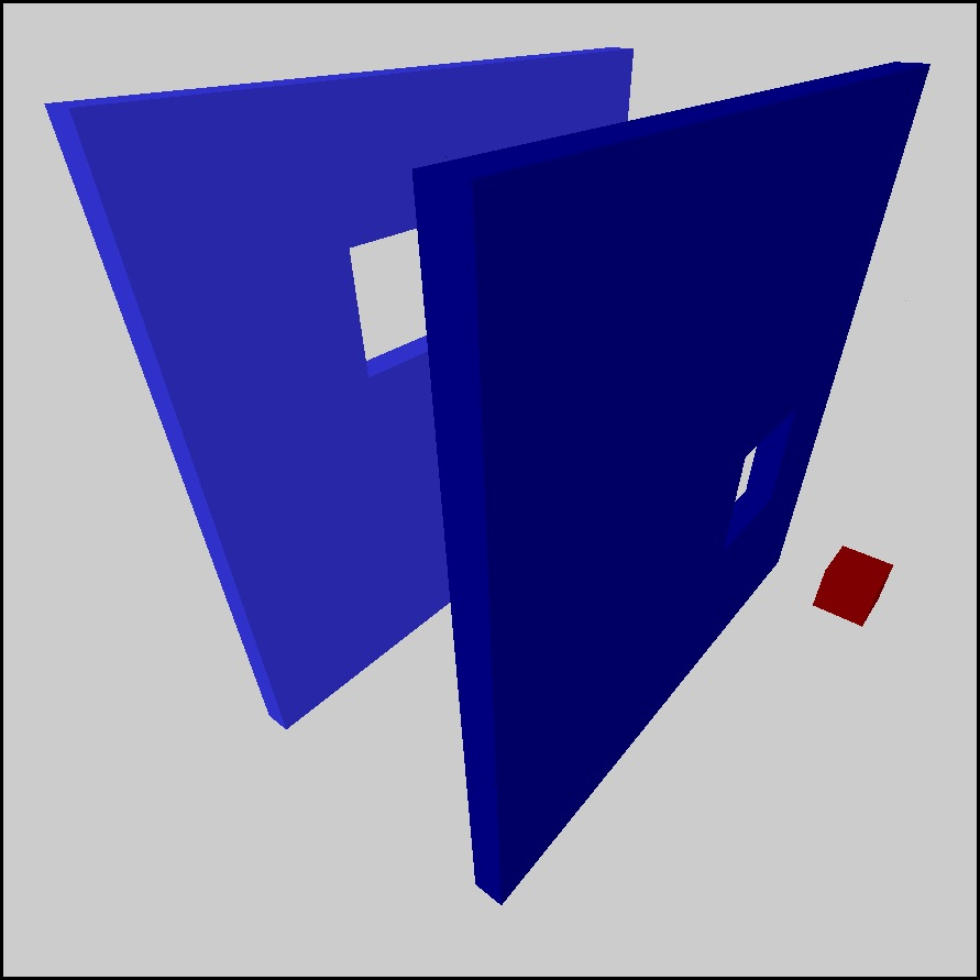
Figure 7: The setup for validating the stopping criterion, for a 3D rigid body without rotations.

To test the validity of the analysis, experiments were performed using the described ${\tt PRM}^{*}$ in the environment illustrated in Figure 7. Experiments were run using the PRACSYS Library Kimmel et al. (2012). The automated stopping criterion was tested to ensure it stops ${\tt PRM}^{*}$ appropriately. The automated stopping criterion should stop the algorithm at an iteration when the ${\tt PNO}$ condition is satisfied, and not let the algorithm run excessively longer than required.

The results of running the stopping criterion are summarized in Figure 8. For the desired path bound and probability of success, the iteration limit $n_{0}$ was computed. Then, out of 1000 experimental trials, the actual probability of successfully generating a path through the set of hyperballs over $\pi_{0}$ is computed. The stopping criterion properly selects $n_{0}$ so that the $\mathbb{P}_{success}$ is greater than the input threshold $\mathbb{P}_{DES}$. The probability of success for the algorithm over time is given in Figure 9 for the two settings of $\mathbb{P}_{DES}$.

${\epsilon_{0}}$	$n_{0}$	$\delta_{DES}$	$\mathbb{P}_{DES}$	$\mathbb{P}_{success}$
0.5	69429	0.16	0.9	0.93
0.5	108328	0.25	0.99	0.998

Figure 8: Results for the 3D Rigid Body scenario. The automated stopping criterion terminates execution to appropriately ensure $\mathbb{P}_{success}\geq\mathbb{P}_{DES}$.

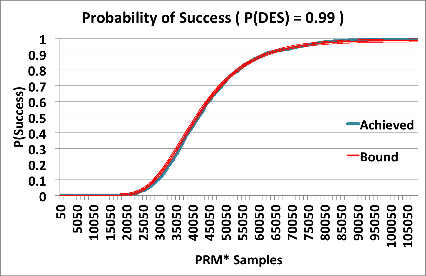
Figure 9: Probability of successfully returning a path within the bound $\delta_{DES}$ for ${\tt PRM}^{*}$ over time.

6 Discussion

This work formally shows ${\tt PNO}$ properties for an asymptotically optimal sampling-based planner, overcoming limitations of prior work. The new framework shows ${\tt PNO}$ properties using an asymptotically sparser planning structure, and removes dependence on Monte Carlo simulations. The analysis shows tight bounds for path quality, and experimental results show that these properties practically guarantee high-quality solutions in finite time.

There are many avenues for future investigation. An important step is to ensure that ${\tt PNO}$ properties can be extended to the tree-based planner ${\tt RRT}^{*}$. Furthermore, these methods still require a large amount of samples, so it is pertinent to determine how ${\tt PNO}$ properties can be extended to roadmap spanner techniques which remove nodes from the planning structure Dobson and Bekris (2014). The drawn bounds reason over a single path which exists in the planning structure, however, less conservative bounds can be drawn if many paths can be considered simultaneously. It is also interesting to see if ${\tt PNO}$ properties can be leveraged to better inform task planners of problem difficulty along different exploration directions. Furthermore, the approach will become more broadly applicable if the bound can be generalized for non-$L_{2}$ norms. The drawn bounds can also be improved, for instance, by computing an analytical solution instead of the approximate bounds computed here, by considering the effects of having multiple samples in each hyperball, or by finding tighter bounds where Chebyshev’s Inequality was employed. An interesting prospect is to investigate low-dispersion sampling approaches, which can effectively ensure that the algorithm always generates samples within the hyperballs.

References

• Amato et al. (1998) N. M. Amato, O. B. Bayazit, L. K. Dale, C. Jones, and D. Vallejo. OBPRM: An Obstacle-based PRM for 3D Workspaces. In WAFR, pages 155–168, 1998.
• Chaudhuri and Koltun (2009) S. Chaudhuri and V. Koltun. Smoothed Analysis of Probabilistic Roadmaps. Computational Geometry, 42(8):731 – 747, 2009. ISSN 0925-7721. doi: http://dx.doi.org/10.1016/j.comgeo.2008.10.005.
• Choset et al. (2005) H. Choset, K. M. Lynch, S. Hutchinson, G. Kantor, W. Burgard, L. E. Kavraki, and S. Thrun. Principles of Robot Motion: Theory, Algorithms, and Implementations. MIT Press, Boston, MA, 2005.
• Dobson and Bekris (2013) A. Dobson and K. E. Bekris. A Study on the Finite-Time Near-Optimality Properties of Sampling-Based Motion Planners. Tokyo Big Sight, Tokyo, Japan, November 2013. IROS.
• Dobson and Bekris (2014) A. Dobson and K. E. Bekris. Sparse Roadmap Spanners for Asymptotically Near-Optimal Motion Planning. IJRR, 33, 01/2014 2014.
• Grimmet and Stirzaker (2001) G. Grimmet and D. Stirzaker. Probability and Random Processes. Oxford University Press, 2001.
• Hsu et al. (1998) D. Hsu, L. Kavraki, J.-C. Latombe, R. Motwani, and S. Sorkin. On Finding Narrow Passages with Probabilistic Roadmap Planners. In WAFR, Houston, TX, 1998.
• Karaman and Frazzoli (2010) S. Karaman and E. Frazzoli. Incremental Sampling-based Algorithms for Optimal Motion Planning. In RSS, Zaragoza, Spain, 2010.
• Karaman and Frazzoli (2011) S. Karaman and E. Frazzoli. Sampling-based Algorithms for Optimal Motion Planning. IJRR, 30(7):846–894, June 2011.
• Kavraki and Latombe (1998) L. E. Kavraki and J.-C. Latombe. Probabilistic Roadmaps for Robot Path Planning, pages 33–53. John Wiley, 1998.
• Kavraki et al. (1996) L. E. Kavraki, P. Svestka, J.-C. Latombe, and M. Overmars. Probabilistic Roadmaps for Path Planning in High-Dimensional Configuration Spaces. IEEE TRA, 12(4):566–580, 1996.
• Kavraki et al. (1998) L. E. Kavraki, M. N. Kolountzakis, and J.-C. Latombe. Analysis of Probabilistic Roadmaps for Path Planning. IEEE TRA, 14(1):166–171, 1998.
• Kimmel et al. (2012) A. Kimmel, A. Dobson, Z. Littlefield, A. Krontiris, J. Marble, and K. E. Bekris. PRACSYS: An Extensible Architecture for Composing Motion Controllers and Planners. In SIMPAR, Tsukuba, Japan, 11/2012 2012.
• Ladd and Kavraki (2004) A. M. Ladd and L. E. Kavraki. Measure Theoretic Analysis of Probabilistic Path Planning. IEEE TRA, 20(2):229–242, April 2004.
• Latombe (1991) J.-C. Latombe. Robot Motion Planning. Kluwer Academic Publishers, Boston, MA, 1991.
• LaValle (1998) S. LaValle. Rapidly-exploring random trees: A new tool for path planning, 1998.
• LaValle (2006) S. M. LaValle. Planning Algorithms. Cambridge University Press, 2006.
• LaValle and Kuffner (2000) S. M. LaValle and J. J. Kuffner. Rapidly-exploring random trees: Progress and prospects. WAFR, 2000.
• Marble and Bekris (2013) J. Marble and K. E. Bekris. Asymptotically Near-Optimal Planning with Probabilistic Roadmap Spanners. IEEE Transactions on Robotics, 29:432–444, 2013.
• McCarthy et al. (2012) Z. McCarthy, T. Bretl, and S. Hutchinson. Proving path non-existence using sampling and alpha shapes. In ICRA, May 2012.
• Raveh et al. (2011) B. Raveh, A. Enosh, and D. Halperin. A Little More, a Lot Better: Improving Path Quality by a Path-Merging Algorithm. IEEE TRO, 27(2):365–370, 2011.
• Salzman and Halperin (2013) O. Salzman and D. Halperin. Asymptotically Near-Optimal RRT for Fast, High-quality Motion Planning. Technical report, arXiv, 2013.
• Santalo (1976) L. A. Santalo. Integral Geometry and Geometric Probability, volume 1 of Encyclopedia of Mathematics and its Applications. Addison-Wesley Publishing Company, Reading, Massachusets, 1976.
• Valiant (1984) L. G. Valiant. A theory of the learnable. Communications of the ACM, 27(11):1134–1142, 1984.
• Varadhan and Manocha (2005) G. Varadhan and D. Manocha. Star-shaped Roadmaps: A Deterministic Sampling Approach for Complete Motion Planning. RSS, 2005.
• Wang et al. (2013) W. Wang, D. Balkcom, and A. Chakrabarti. A fast streaming spanner algorithm for incrementally constructing sparse roadmaps. In ICRA, 2013.
• Wilmarth et al. (1999) S. A. Wilmarth, N. M. Amato, and P. F. Stiller. MAPRM: A Probabilistic Roadmap Planner with Sampling on the Medial Axis of the Free Space. In ICRA, pages 1024–1031, Detroit, MI, May 1999.