Energy spectrum of Buoyancy-driven Flows

Abstract

Using high-resolution direct numerical simulation and arguments based on the kinetic energy flux $\Pi_{u}$, we demonstrate that for stably stratified flows, the kinetic energy spectrum $E_{u}(k)\sim k^{-11/5}$, the entropy spectrum $E_{\theta}(k)\sim k^{-7/5}$, and $\Pi_{u}(k)\sim k^{-4/5}$ (Bolgiano-Obukhov scaling). This scaling is due to the depletion of kinetic energy because of buoyancy. For weaker buoyancy in stratified flows, $E_{u}(k)$ follows Kolmgorov’s spectrum with a constant energy flux. We also argue that for Rayleigh Bénard convection, the Bolgiano-Obukhov scaling will not hold for the bulk flow due to the positive energy supply by buoyancy and non-decreasing $\Pi_{u}(k)$.

Buoyancy or density gradient drives flows in the atmosphere and interiors of planets and stars, as well as in electronic devices and industrial applications like heat exchangers, boilers, etc. Accordingly, scientists (including geo-, astro-, atmospheric- and solar physicists) and engineers have been working on understanding buoyancy driven flows for more than a century. An important unsolved problem in this field is how to quantify the spectra and fluxes of kinetic energy (KE) and entropy ($u^{2}/2$ and $\theta^{2}/2$ respectively, where $\mathbf{u}$ and $\theta$ are the velocity and temperature fluctuations) of buoyancy driven flows Siggia (1994); Lohse and Xia (2010). In this letter, we will study these quantities and respective nonlinear fluxes using direct numerical simulations, and show that the spectrum differs from Kolmogorov’s theory when buoyancy is strong.

Flows driven by buoyancy can be classified in two categories: (a) convective flows in which hotter and lighter fluid at the bottom rises, while colder and heavier fluid at the top comes down. These flows are unstable; (b) Stably stratified flows in which lighter fluid rests above heavier fluid. Stably stratified flows are stable, hence their fluctuations vanish over time. Therefore, they need to be driven by an external force to obtain a steady turbulent state. Even though both types of flows are driven by density gradients, the properties of such flows are quite different, which we decipher using quantitative analysis of energy flux and energy supply rate by buoyancy.

For stably stratified flows, Bolgiano Bolgiano (1959) and Obukhov Obukhov (1959) first proposed a phenomenology, according to which the KE flux $\Pi_{u}$ of a stably stratified flow is depleted at different length scales due to conversion of kinetic energy to “potential energy” via buoyancy ($u_{z}\theta$). As a result, $\Pi_{u}(k)$ decreases with wavenumber (see Fig. 1(a)), and the energy spectrum is steeper than that prediced by Kolmogorov theory $(E(k)\sim k^{-5/3}$, where $k$ is the wavenumber). According to the phenomenology proposed by Bolgiano and Obukbhov (referred to as BO), for $k<k_{B}$ ($k_{B}=$ Bolgiano wavenumber Bolgiano (1959)), the KE spectrum $E_{u}(k)$, entropy spectrum $E_{\theta}(k)$, $\Pi_{u}$, and entropy flux $\Pi_{\theta}$ are:

$$E_{u}(k) = c_{1}(\alpha^{2}g^{2}\epsilon_{\theta})^{2/5}k^{-11/5},$$ (1)

$$E_{\theta}(k) = c_{2}(\alpha g)^{-2/5}\epsilon_{\theta}^{4/5}k^{-7/5},$$ (2)

$$\Pi_{\theta}(k) = \epsilon_{\theta}=\mathrm{constant},$$ (3)

$$\Pi_{u}(k) = c_{3}(\alpha^{2}g^{2}\epsilon_{\theta})^{3/5}k^{-4/5},$$ (4)

where $\alpha$, $g$, and $\epsilon_{\theta}$ are the thermal expansion coefficient, acceleration due to gravity, and the entropy dissipation rate respectively, and $c_{i}$’s are constants.

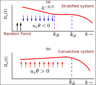
Figure 1: Schematic diagrams of energy flux $\Pi_{u}(k)$: (a) In a stably stratified flow, $\Pi_{u}(k)$ decreases with $k$ due to a negative energy supply rate $\Re\langle u_{z}(k)\theta^{*}(k)\rangle$. (b) In a thermally driven flow (e.g., Rayleigh Bénard convection), $\Pi_{u}(k)$ is a non-decreasing function of $k$ due to positive $\Re\langle u_{z}(k)\theta^{*}(k)\rangle$.

According to the BO theory, the decrease in $\Pi_{u}(k)$ occurs due to a negative energy supply rate $F(k)=\Re\langle u_{z}(k)\theta^{*}(k)\rangle$, where $\Re$ stands for the real part of the argument. For the wavenumbers in the range $k_{B}<k<k_{d}$, $\Pi_{u}\approx\epsilon_{u}$, and $E_{u}(k),E_{\theta}(k)\sim k^{-5/3}$ (see Fig. 1(a)). Here $\epsilon_{u}$ is the KE dissipation rate, and $k_{d}$ is the wavenumber after which dissipation starts. In this letter we numerically compute $F(k)$ and $\Pi_{u}(k)$ for stratified turbulence, and show a consistency with the BO scaling. We remark that many researchers describe the stably stratified flows in terms of density fluctuation $\rho^{\prime}$, which leads to an equivalent description since $\theta^{2}/2$ is proportional to $\rho^{\prime 2}/2$ (usually referred to as “potential energy” Davidson (2013)).

Procaccia and Zeitak Procaccia and Zeitak (1989), L’vov L’vov (1991), L’vov and Falkovich L’vov and Falkovich (1992), and Rubinstein Rubinstein (2013) proposed that a similar scaling is applicable to Rayleigh-Bénard convection (RBC). Their arguments hinges on an assumption that $F(k)=\Re\langle u_{z}(k)\theta^{*}(k)\rangle<0$ even for RBC. Note that for the inertial range regime, under a steady state, the variation of energy flux is given by

$$\frac{d}{dk}\Pi(k)=F(k)-D(k),$$ (5)

where $D(k)$ is the viscous dissipation L’vov (1991); L’vov and Falkovich (1992); Lesieur (2008); Verma (2012); suppl . In this letter, we demonstrate using numerical simulations that $F(k)>0$ for RBC [see Fig. 1(b)], unlike stably stratified flows where $F(k)<0$. Consequently $\Pi(k)$ would increase with $k$, and $E(k)$ would be either Kolmogorov-like ($E(k)\sim k^{-5/3}$) or shallower ($E(k)\sim k^{-a}$ with $a<5/3$). These observations of non-decreasing $\Pi(k)$ contradict the earlier predictions on RBC Procaccia and Zeitak (1989); L’vov (1991); L’vov and Falkovich (1992), but they are in agreement with the numerical results of Škandera et al. Škandera et al. (2008).

In the past there have been several attempts to verify BO scaling for stably stratified flows. Kimura and Herring Kimura and Herring (1996) reported BO scaling for a narrow band of wavenumbers in their $128^{3}$ decaying spectral simulation; the Richardson number of their simulations was greater than unity. Later, Kimura et al. Kimura and Herring (2012), Lindborg Lindborg (2005, 2006), and Vallgren et al. Vallgren et al. (2011) focussed on anisotropic energy spectrum, and attempted to explain $k^{-3}$ KE spectrum observed for the synoptic scale of terrestrial atmosphere.

For Rayleigh Bénard convection (RBC), which is a class of thermally-driven convection, the numerical and experimental results are largely inconclusive. Based on simulations with periodic boundary conditions, Borue and Orszag Borue and Orszag (1997) and Škandera et al. Škandera et al. (2008) reported KO scaling. Škandera et al. Škandera et al. (2008) reported a constant KE flux, somewhat consistent with the aforementioned argument [Eq. (5)]. Calzavarini et al. Calzavarini et al. (2002) reported BO scaling in the boundary layer, and KO scaling in the bulk. Mishra and Verma Mishra and Verma (2010) reported KO scaling for zero- and low Prandtl number flows since $F(k)=\Re\langle u_{z}(k)\theta^{*}(k)\rangle$ is active only at low wavenumbers for such flows. Camussi and Verzicco Camussi and Verzicco (2004); Verzicco and Camussi (2003) however reported BO scaling. The experimental results Niemela et al. (2000) are more divergent with some reporting BO scaling, and some reporting KO scaling.

In this letter, we focus on Boussinesq stably stratified flows, whose equations in a non-dimensionalised form are

$$\frac{\partial\bf u}{\partial t}+(\bf u\cdot\nabla)\bf u = -\nabla\sigma+\mathrm{Gr}\mathrm{Pr}^{2}\theta\hat{z}+\mathrm{Pr}\nabla^{2}\bf u+\bf f^{u},$$ (6)

$$\frac{\partial\theta}{\partial t}+(\bf u\cdot\nabla)\theta = -u_{z}+\nabla^{2}\theta,$$ (7)

$$\nabla\cdot\bf u = 0,$$ (8)

where $\mathrm{Pr=\nu/\kappa}$ is the Prandtl number, and $\mathrm{Gr}=\alpha g\frac{dT}{dz}d^{4}/\nu^{2}$ is the Grashof number, which is a ratio of the buoyancy and dissipation terms. Another important non-dimensional number is Richardson number $\mathrm{Ri}=\alpha g\frac{dT}{dz}d^{2}/u_{\rm rms}^{2}$, which is a ratio of the buoyancy and the nonlinear term $(\bf u\cdot\nabla)\bf u$. We demonstrate that BO scaling is observed when $\mathrm{Ri}=O(1)$, but Kolmogorov scaling $E(k)\sim k^{-5/3}$ [referred to as Kolmogorov-Obukhov (KO) scaling] is observed when $\mathrm{Ri}\ll 1$, or when buoyancy is negligible.

To test whether BO scaling is valid or not for the stably stratified flows, we perform direct numerical simulation of Eqs. (6-8) using pseudospectral code Tarang Verma et al. (2013) in a three-dimensional box of size $(2\pi)^{3}$. We employ periodic boundary condition on all sides Kimura and Herring (2012). We use fourth-order Runge-Kutta (RK4) method for time stepping, Courant-Freidricks-Lewey (CFL) condition for computing time step $\Delta t$, and $3/2$ rule for dealiasing. To obtain a steady turbulent flow, we apply a random force to the flow in the band $2\leq k\leq 4$ using the scheme of Kimura and Herring Kimura and Herring (2012).

We perform large-resolution simulations for $\mathrm{P}r=1$ (close to that of air) and Richardson numbers $\mathrm{Ri}=4\times 10^{-7},0.01$, and $0.5$. Simulations for $\mathrm{Ri}=0.01$ have been performed on $1024^{3}$ grid, while that for $4\times 10^{-7}$ and $0.5$ have been performed on $512^{3}$ grid. The parameters of our runs are listed in Table 1. All our simulations are fully resolved since $k_{\mathrm{m}ax}\eta>1$, where $k_{\mathrm{m}ax}$ is the maximum wavenumber of the run, and $\eta$ is the Kolmogorov length scale.

Table 1: Parameters of our numerical simulations: Richardson number $\mathrm{Ri}$, Grashof number $\mathrm{Gr}$, Prandtl number $\mathrm{Pr}$, Grid size, kinetic energy dissipation rate $\epsilon_{u}$, thermal dissipation rate $\epsilon_{\theta}$, Reynolds number $\mathrm{Re}$, Reynolds number $\mathrm{Re_{\lambda}}$ based on Taylor micro-scale, $k_{max}\eta$ where $\eta$ is the Kolmogorov length, Bolgiano wavenumber $k_{B}$, and averaged $\Delta t$.

$\mathrm{Ri}$	$\mathrm{Gr}$	$\mathrm{Pr}$	Grid	$\epsilon_{u}$	$\epsilon_{\theta}$	$\mathrm{Re}$	$\mathrm{Re_{\lambda}}$	$k_{max}\eta$	$k_{B}$	$\Delta t$
$0.5$	$1\times 10^{5}$	$1$	$512^{3}$	$1.4\times 10^{7}$	$60.7$	$467$	$220$	$4.2$	$6.0$	$2.5\times 10^{-5}$
$0.01$	$5\times 10^{3}$	$1$	$1024^{3}$	$4.0\times 10^{7}$	$150$	$649$	$260$	$6.4$	$8.5$	$3.5\times 10^{-6}$
$4\times 10^{-7}$	$0.1$	$1$	$512^{3}$	$2.1\times 10^{7}$	$141$	$510$	$220$	$3.8$	$<1$	$2.6\times 10^{-6}$

We compute the KE and entropy spectra and fluxes for the steady-state data of $\mathrm{Pr}=1$ and $\mathrm{Ri}=0.01$ run. In Fig. 2(a) we plot the normalized KE spectra, $E_{u}(k)k^{11/5}$ (BO scaling) and $E_{u}(k)k^{5/3}$ (KO scaling). In Fig. 2(b) we plot the normalized entropy spectra, $E_{\theta}(k)k^{7/5}$ (BO scaling) and $E_{\theta}(k)k^{5/3}$ (KO scaling). The figures indicate that for $\mathrm{Ri}=0.01$, BO scaling fits with the numerical data better than KO scaling.

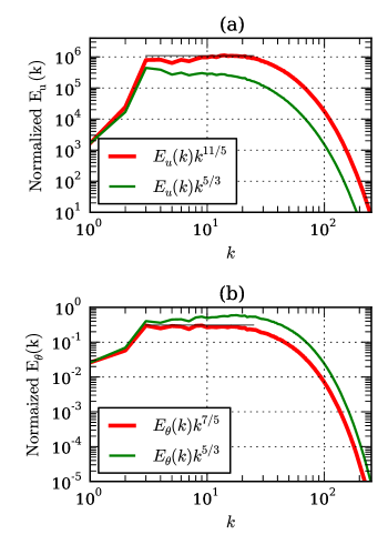
Figure 2: For $\mathrm{Pr}=1$ and $\mathrm{Ri}=0.01$, plots of (a) normalized KE spectra and (b) normalized entropy spectra for Bolgiano-Obukhov (BO) and Kolmogorov-Obukhov (KO) scaling. BO scaling fits with the data better than KO scaling.

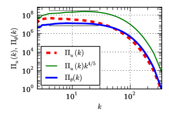
Figure 3: For $\mathrm{Pr}=1$ and $\mathrm{Ri}=0.01$, plots of KE flux $\Pi_{u}(k)$, normalized KE flux $\Pi_{u}(k)k^{4/5}$, and entropy flux $\Pi_{\theta}(k)$. $\Pi_{\theta}(k)$ is multiplied by $10^{5}$ to fit in the same plot.

We cross check our spectrum results with those on KE and entropy fluxes, which are plotted in Fig. 3. Clearly, the KE flux $\Pi_{u}(k)$ is positive, and it decreases with $k$. However $\Pi_{u}(k)k^{4/5}$ is almost flat, thus $\Pi_{u}(k)\propto k^{-4/5}$, consistent with the BO predictions [Eq. (4)]. This is consistent with the observed negative $F(k)=\Re\langle u_{z}(k)\theta^{*}(k)\rangle$ for this case (see Fig. 4 and suppl ). We also observe that $\Pi_{\theta}$ is a constant in the inertial range [Eq. (3)]. These results show that the BO scaling is valid for stably stratified flows for $\rm Ri=O(1)$. We also compute the Bolgiano wavenumber $k_{B}$ Bolgiano (1959) using the numerical data of Eq. (4), and find that $k_{B}\approx 8.5$. Our plots on spectra and fluxes show that $k_{B}\approx 8.5$ is only 3 to 4 times smaller than $k_{d}$, wavenumber where the dissipation range starts. Therefore a clear-cut crossover from $k^{-11/5}$ to $k^{-5/3}$ is not observed in our simulations. We are in the process of performing simulations on even higher resolution to probe the crossover region.

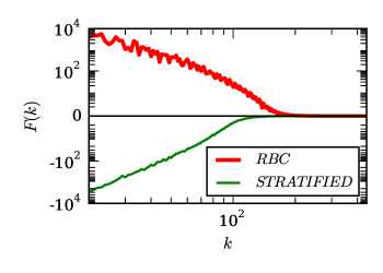
Figure 4: Plots of $F(k)$ stably stratified flow ($\mathrm{Pr}=1$, $\mathrm{Ri}=0.01$ on $1024^{3}$ grid), and for RBC ($\mathrm{Pr}=1$, $\mathrm{Ra}=5\times 10^{6}$ on $256^{3}$ grid). $F(k)<0$ for stratified flows, but $F(k)>0$ for RBC. $F(k)$ for RBC is multiplied by $10^{4}$ to fit in the same plot.

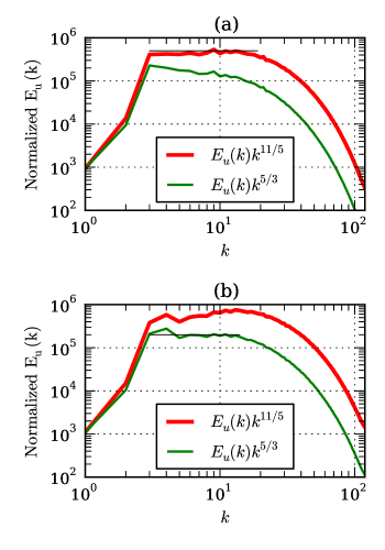
Figure 5: Plots of normalized KE spectra for Bolgiano-Obukhov (BO) scaling and Kolmogorov-Obukhov (KO) scaling for: (a) $\mathrm{Ri}=0.5$ and (b) $\mathrm{Ri}=4\times 10^{-7}$

We also performed $512^{3}$ grid simulations for ${\rm Ri}=0.5$ and $4\times 10^{-7}$ with $\mathrm{Pr}=1$. The normalized KE spectra for these two cases are exhibited in Figs. 5(a) and  5(b) respectively. Our results show that BO scaling is valid for ${\rm Ri}=0.5$, but KO scaling (with a constant $\Pi_{u}(k)$) is valid for ${\rm Ri}=4\times 10^{-7}$, which is as expected since buoyancy is significant only for moderate and large ${\rm Ri}$’s. The energy supply rate by buoyancy, $F(k)$, is significant for ${\rm Ri}=0.5$, but insignificant for ${\rm Ri}=4\times 10^{-7}$, consistent with the above observations suppl .

To contrast the energy supply rate by buoyancy in stratified flows with that in Rayleigh Bénard convection (RBC), we numerically solve the nondimensionalized RBC equations for $\mathrm{Pr}=1.0$ and Rayleigh number $\mathrm{Ra}=5\times 10^{6}$ on $256^{3}$ grid Mishra and Verma (2010). For this run, we plot $F(k)$ in Fig. 4 that demonstrates that $F(k)>0$, consistent with our aforementioned arguments, but differs from those of L’vov and Falkovich L’vov and Falkovich (1992). The ongoing work on the flux and spectrum for RBC will be reported in a future work. Thus, the behaviour of $F(k)$ and $\Pi_{u}(k)$ for the stably stratified flow and RBC are quite different.

We employ periodic boundary condition for the stably stratified flows in the vertical direction, thus eliminating the effects of boundary walls. In Fig. 6 we plot the plane-averaged mean temperature profile $\bar{T}(z)=\langle T(x,y,z)\rangle_{xy}$. Since $\bar{T}(z)$ is linear, a constant temperature gradient $d\bar{T}/dz$ (hence buoyancy) acts in the whole box. Therefore, BO scaling is expected everywhere. It is important to contrast the above profile with that for Rayleigh-Bénard convection in which most of the temperature drop takes place in a narrow thermal boundary layer Moore and Weiss (1973); Verzicco and Camussi (2003), while the bulk flow has $d\bar{T}/dz\approx 0$. Thus we expect BO scaling in the boundary layers, and KO scaling in the bulk, as reported by Calzavarini et al. Calzavarini et al. (2002).

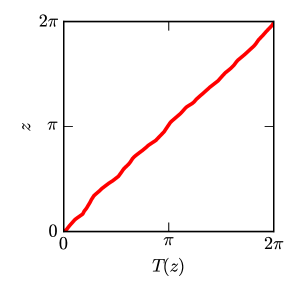
Figure 6: The vertical variation of horizontally averaged mean temperature $\bar{T}(z)=\langle T(x,y,z)\rangle_{xy}$ for $\mathrm{Pr}=1$ and $\mathrm{Ri}=0.01$ run.

In summary, our numerical simulations demonstrate an existence of BO scaling in stably stratified flows. A major novelty in our approach is the quantitative analysis of the KE and entropy fluxes, as well as the energy supply rate by buoyancy ($F(k)$). We show that $F(k)<0$ for stably stratified flows, but $F(k)>0$ for Rayleigh Bénard convection. Consequently, for stably stratified flows with moderate Richardson numbers, the energy flux $\Pi_{u}(k)\propto k^{-4/5}$ and $E_{u}(k)\sim k^{-11/5}$, as proposed in the BO phenomenology. However, $F(k)$ is somewhat insignificant for small Richardson number, and we observe KO scaling. For RBC flows, $\Pi_{u}(k)$ is a non-decreasing function of $k$ (since $F(k)>0$), and the energy spectrum of KE cannot be steeper than $k^{-5/3}$ in the bulk. Thus, energy flux and energy supply rate due to buoyancy provide valuable insights into the physics of stably stratified flows and RBC.

Our numerical simulations were performed at Centre for Development of Advanced Computing (CDAC) and IBM Blue Gene P “Shaheen” at KAUST supercomputing laboratory, Saudi Arabia. This work was supported by a research grant SERB/F/3279/2013-14 from Science and Engineering Research Board, India. We thank Ambrish Pandey, Anindya Chatterjee, Pankaj Mishra, and Mani Chandra for valuable suggestions.

I Supplemental Material

In Fourier space, the equation for the kinetic energy (KE) can be derived from Eq. (1) of the main paper as Lesieur (2008); L’vov (1991); Verma (2012)

$$\frac{\partial E_{u}(k)}{\partial t}=T_{u}(k)+F(k)-D(k)$$ (9)

where $T_{u}(k)$ is energy transfer rate to a wavenumber shell of radius $k$, and it is related to the energy flux of KE as

$$\Pi_{u}(k)=-\int_{0}^{k}T_{u}(k)\,dk.$$ (10)

The energy supply rate $F(k)$ of Eq. (9) is given by

$$F(k)=\mathrm{GrPr^{2}}\sum_{|{\mathbf{k}}|=k}\Re\langle u_{z}({\mathbf{k}})\theta^{*}({\mathbf{k}})\rangle+\Re\langle{\mathbf{u}}({\mathbf{k}})\cdot{\mathbf{f}}^{*}({\mathbf{k}})\rangle,$$ (11)

where the first term is due to buoyancy, while the second term is due to the external random forcing, which is active only for $2\leq k\leq 4$. The viscous dissipation is given by

$$D(k)=\sum_{|{\mathbf{k}}|=k}2\mathrm{Pr}k^{2}E_{u}(k)$$ (12)

From the above equation, we deduce that

$$\frac{d}{dk}\Pi(k)=-T(k)=-\frac{\partial E}{\partial t}+F(k)-D(k).$$ (13)

Under a steady state ($\partial E/\partial t=0$), we obtain

$$\frac{d}{dk}\Pi(k)=F(k)-D(k).$$ (14)

In our simulations of stably stratified flows, the external force ${\mathbf{f}}^{*}({\mathbf{k}})$ is active for the band $2\leq k\leq 4$. Therefore, we focus on wavenumbers $k>4$ where only buoyancy force is active.

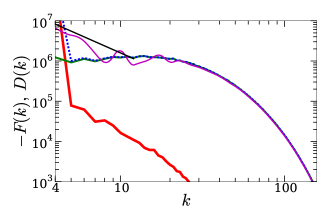
Figure 7: For $\mathrm{Pr}=1$ and $\mathrm{Ri}=0.01$, plots of $-F(k)$ (thick red curve), $D(k)$ (thick green curve), $[-F(k)+D(k)]$ (dotted blue curve) , and $-\frac{d}{dk}\Pi_{u}(k)$ (thin magenta curve). $k^{-9/5}$ scaling is shown using black line.

We compute $F(k)$ and $D(k)$ using the numerical data computed for stably stratified flows with $\mathrm{Pr}=1$, and $\mathrm{Ri}=0.01,0.5,4\times 10^{-7}$. These quantities are shown in Figs. 7, 8, and 9 respectively. In the inertial range, $F(k)$ is negative for all the three cases, consistent with the predictions of Bolgiano-Obukhov (BO) phenomenology. We observe that for $\mathrm{Ri}=0.01$ and $0.5$, $F(k)$ is significant for small wavenumbers. However for $\mathrm{Ri}=4\times 10^{-7}$, buoyancy is weak, and $|F(k)|\ll D(k)$. These results are consistent with the flux and spectra results presented in the main paper.

We also find that $|F(k)|$ drops sharply with $k$ for $\mathrm{Ri}=0.01,0.5$. Since $\Pi(k)\sim k^{-4/5}$, we observe $F(k)\sim d\Pi/dk\sim-k^{-9/5}$ for a narrow band in the small wavenumber regime. In contrast, for $\mathrm{Ri}=4\times 10^{-7}$, $F(k)$ is much smaller than the corresponding $F(k)$ for $\mathrm{Ri}=0.01,0.5$, consistent with $d\Pi(k)/dk\approx-D(k)$.

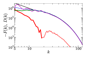
Figure 8: For $\mathrm{Pr}=1$ and $\mathrm{Ri}=0.5$, $F(k)$ has both signs. We exhibit negative $F(k)$ (lower $k$) with thick red curve, and positive $F(k)$ (higher $k$) using thick dotted red curve. We also exhibit $D(k)$ (thick green curve), $[-F(k)+D(k)]$ (thick dotted blue curve), and $-\frac{d}{dk}\Pi_{u}(k)$ (thin magenta curve). $k^{-9/5}$ scaling is shown using black line.

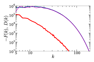
Figure 9: For $\mathrm{Pr}=1$ and $\mathrm{Ri}=4\times 10^{-7}$, plots of $-F(k)$ (thick red curve), $D(k)$ (thick green curve), $[-F(k)+D(k)]$ (dotted blue curve) , and $-\frac{d}{dk}\Pi_{u}(k)$ (thin magenta curve). $F(k)$ is multiplied by $10^{5}$ to fit in the same plot.

We contrast the above results with those for Rayleigh Bénard convection (RBC). We numerically solve the nondimensionalized RBC equations under the Boussinesq approximation for $\mathrm{Pr}=1.0$ and Rayleigh number $\mathrm{Ra}=5\times 10^{6}$ on $256^{3}$ grid Mishra and Verma (2010). For this run, we plot $F(k)$ and $D(k)$ in Fig. 10 that demonstrates that $F(k)>0$, consistent with our arguments. Note however that for this case, $F(k)\ll D(k)$ and $d\Pi_{u}(k)/dk=-D(k)<0$, or $\Pi_{u}(k)$ is decreasing with $k$ due to dominance of $D(k)$ over $F(k)$. We need to perform very large-resolution simulation for much higher $\mathrm{Ra}$ that would provide significant inertial range where $\Pi_{u}(k)$ could be a non-decreasing function of $k$.

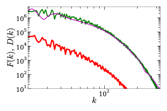
Figure 10: For $\mathrm{Pr}=1$ and $\mathrm{Ra}=5\times 10^{6}$, plots of $F(k)$ (thick red curve), $D(k)$ (thick green curve), and $-\frac{d}{dk}\Pi_{u}(k)$ (thin magenta curve) on $256^{3}$ grid. $F(k)$ is multiplied by $10^{5}$ to fit in the same plot.

References

- Siggia (1994) E. D. Siggia, Ann. Rev. Fluid Mech. 26, 137 (1994).
- Lohse and Xia (2010) D. Lohse and K. Q. Xia, Ann. Rev. Fluid Mech. 42, 335 (2010).
- Bolgiano (1959) R. Bolgiano, J. Geophys. Res. 64, 2226 (1959).
- Obukhov (1959) A. N. Obukhov, Dokl. Akad. Nauk SSSR 125, 1246 (1959).
- Davidson (2013) P. A. Davidson, Turbulence in Rotating Stratified and Electrically Conducting Fluids (Cambridge university press, Cambridge, 2013).
- Procaccia and Zeitak (1989) I. Procaccia and R. Zeitak, Phys. Rev. Lett. 62, 2128 (1989).
- L’vov (1991) V. S. L’vov, Phys. Rev. Lett. 67, 687 (1991).
- L’vov and Falkovich (1992) V. S. L’vov and G. E. Falkovich, Physica D 57, 85 (1992).
- Rubinstein (2013) R. Rubinstein, ICQMP-94-8; CMOTT-94-2 (NASA Technical Memorandum 1066602, 1994).
- Lesieur (2008) M. Lesieur, Turbulence in Fluids - Stochastic and Numerical Modelling (Kluwer Academic Publishers, Dordrecht, 2008), 4th ed.
- Verma (2012) M. K. Verma, Europhys Lett 98, 14003 (2012).
- (12) See Supplemental Materials for plots of ,, , and for stratified flow at and (Figs. (1-3)), and convective flows at (Fig. (4)).
- Škandera et al. (2008) D. Škandera, A. Busse, and W. C. Müller, High Performance Computing in Science and Engineering, Transactions of the Third Joint HLRB and KONWIHR Status and Result Workshop (Springer, Berlin), Part IV, p. 387 (2008).
- Kimura and Herring (1996) Y. Kimura and J. R. Herring, J. Fluid Mech. 328, 253 (1996).
- Kimura and Herring (2012) Y. Kimura and J. R. Herring, J. Fluid Mech. 698, 19 (2012).
- Lindborg (2005) E. Lindborg, Geo. Res. Lett. 32, 207 (2005).
- Lindborg (2006) E. Lindborg, J. Fluid Mech. 550, 207 (2006).
- Vallgren et al. (2011) A. Vallgren, E. Deusebio, and E. Lindborg, Phys. Rev. Lett. 107, 268501 (2011).
- Borue and Orszag (1997) V. Borue and S. A. Orszag, J. Sci. Comput. 12, 305 (1997).
- Calzavarini et al. (2002) E. Calzavarini, F. Toschi, and R. Tripiccione, Phys. Rev. E 66, 016304 (2002).
- Mishra and Verma (2010) P. K. Mishra and M. K. Verma, Phys. Rev. E 81, 056316 (2010).
- Camussi and Verzicco (2004) R. Camussi and R. Verzicco, Eur. J. of Mech. /B Fluids 23, 427 (2004).
- Verzicco and Camussi (2003) R. Verzicco and R. Camussi, J. Fluid Mech. 477, 19 (2003).
- Niemela et al. (2000) X. Z. Wu, L. Kadanoff, A. Libchaber, and M. Sano, Phys. Rev. Lett. 64, 2140 (1990); F. Chillá, S. Ciliberto, C. Innocenti, and E. Pampaloni, Nuovo Cimento D 15, 1229 (1993); S. Cioni, S. Ciliberto, and J. Sommeria, Europhys Lett 32, 413 (1995); J. J. Niemela, L. Skrbek, K. R. Sreenivasan, and R. J. Donnelly, Nature 404, 837 (2000); S. Q. Zhou and K. Q. Xia, Phys. Rev. Lett. 87, 064501 (2001); X. D. Shang and K. Q. Xia, Phys. Rev. E 64, 065301 (2001); T. Mashiko, Y. Tsuji, T. Mizuno, and M. Sano, Phys. Rev. E 69, 036306 (2004); J. Zhang, X. L. Wu, and K. Q. Xia, Phys. Rev. Lett. 94, 174503 (2005); C. Sun, Q. Zhou, and K. Q. Xia, Phys. Rev. Lett. 97, 144504 (2006).
- Verma et al. (2013) M. K. Verma, A. G. Chatterjee, K. S. Reddy, R. K. Yadav, S. Paul, M. Chandra, and R. Samtaney, Pramana 81, 617 (2013).
- Moore and Weiss (1973) D. Moore and N. Weiss, J. Fluid Mech. 58, 289 (1973).

References

- Lesieur (2008) M. Lesieur, Turbulence in Fluids - Stochastic and Numerical Modelling (Kluwer Academic Publishers, Dordrecht, 2008), 4th ed.
- L’vov (1991) V. S. L’vov, Phys. Rev. Lett. 67, 687 (1991)
- Verma (2012) M. K. Verma, Europhys Lett 98, 14003 (2012).
- Mishra and Verma (2010) P. K. Mishra and M. K. Verma, Phys. Rev. E 81, 056316 (2010).