Penguin-dominated $B\to\phi K_{1}(1270)$ and $\phi K_{1}(1400)$ decays in the perturbative QCD approach

Abstract

We investigate the CP-averaged branching ratios, the polarization fractions, the relative phases, and the CP-violating asymmetries of the penguin-dominated $B\to\phi K_{1}(1270)$ and $\phi K_{1}(1400)$ decays in the perturbative QCD(pQCD) approach, where $K_{1}(1270)$ and $K_{1}(1400)$ are believed to be the mixtures of two distinct types of axial-vector $K_{1A}(^{3}P_{1})$ and $K_{1B}(^{1}P_{1})$ states with different behavior, however, their mixing angle $\theta_{K_{1}}$ is still a hot and controversial topic presently. By numerical evaluations with two different mixing angles $\theta_{K_{1}}\sim 33^{\circ}$ and $58^{\circ}$ and phenomenological analysis, we find that: (a) the pQCD predictions for the branching ratio, the longitudinal polarization fraction and the direct CP violation of $B^{\pm}\to\phi K_{1}(1270)^{\pm}$ decay with the smaller angle $33^{\circ}$ are in good agreement with the currently available data; (b) though the central values significantly exceed the available upper limit, both pQCD predictions of $Br(B^{\pm}\to\phi K_{1}(1400)^{\pm})$ with two different mixing angles are consistent with that obtained in QCD factorization and with the preliminary data in 2$\sigma$ errors. These results and other relevant predictions for the considered decays will be further tested by the LHCb and the forthcoming Super-B experiments; (c) the weak annihilation contributions can play an important role in $B\to\phi K_{1}(1270)$ and $\phi K_{1}(1400)$ decays; (d) these pQCD predictions combined with the future precision measurements can examine the reliability of the factorization approach employed here, but also explore the complicated QCD dynamics and mixing angle $\theta_{K_{1}}$ of the axial-vector $K_{1}(1270)$ and $K_{1}(1400)$ system.

I Introduction

In the quark model, the possible quantum numbers $J^{PC}$ for the orbitally excited axial-vector mesons are $1^{++}$ or $1^{+-}$, depending on different spin couplings of the involved two quarks. In the SU(3) limit, those mesons can not mix with each other; but, since the $s$ quark is heavier than $u,d$ quarks, the physical states of strange axial-vector mesons, $K_{1}(1270)$ and $K_{1}(1400)$, are believed to be mixtures of two distinct types of $K_{1A}$ and $K_{1B}$, where $K_{1A}$ and $K_{1B}$ are ${}^{3}P_{1}$ and ${}^{1}P_{1}$ states, respectively. Because both $K_{1}$(Hereafter, for the sake of simplicity, we will adopt $K_{1}$ to denote $K_{1}(1270)$ and $K_{1}(1400)$ unless otherwise stated.) mesons are not pure ${}^{3}P_{1}$ or ${}^{1}P_{1}$ states, the mixing angle $\theta_{K_{1}}$ between two axial-vector states $K_{1A}$ and $K_{1B}$ is now of great interest at both theoretical and experimental aspects. Furthermore, the mixing angle $\theta_{K_{1}}$ can be utilized to determine the mixing angle $\theta_{{}^{1}P_{1}}$ and $\theta_{{}^{3}P_{1}}$ with the former(latter) being the mixing angle of $h_{1}(1170)(f_{1}(1285))$ and $h_{1}(1380)(f_{1}(1420))$ in the flavor basis through mass relations(for detail, see recent discussion Cheng:2013cwa ). However, this mixing angle $\theta_{K_{1}}$ is still an issue in controversy presently. It is therefore definitely interesting to investigate the mixing angle $\theta_{K_{1}}$ through kinds of ways, for example, examining the hints of $\theta_{K_{1}}$ in the rare $B$ meson decays to the final states involving the aforementioned $K_{1}$ mesons.

Recently, the BABAR Collaboration has measured the branching ratio, the longitudinal polarization fraction and the direct CP asymmetry(Here, the definition of the direct CP asymmetry ${\cal A}_{CP}$ is $\frac{\Gamma^{+}-\Gamma^{-}}{\Gamma^{+}+\Gamma^{-}}$ Aubert:2008bc , where $\Gamma^{+}$ and $\Gamma^{-}$ denote the decay width of $B^{+}$ and $B^{-}$ meson, respectively.) of $B^{\pm}\to\phi K_{1}(1270)^{\pm}$ decay Aubert:2008bc for the first time,

$$Br(B^{\pm}\to\phi K_{1}(1270)^{\pm}) = (6.1\pm 1.6\pm 1.1)\times 10^{-6}\;;$$

$$f_{L}(B^{\pm}\to\phi K_{1}(1270)^{\pm}) = 0.46^{+0.12+0.06}_{-0.13-0.07}\;;$$ (1)

$$A_{CP}(B^{\pm}\to\phi K_{1}(1270)^{\pm}) = +0.15\pm 0.19\pm 0.05\;;$$

and placed the upper limit at 90% C.L. on the branching ratio of $B^{\pm}\to\phi K_{1}(1400)^{\pm}$ decay Aubert:2008bc ,

$$Br(B^{\pm}\to\phi K_{1}(1400)^{\pm}) < 3.2(0.3\pm 1.6\pm 0.7)\times 10^{-6}\;.$$ (2)

One can easily observe that the vector-axial-vector $B^{\pm}\to\phi K_{1}(1270)^{\pm}$ decay looks more like the vector-vector $B^{\pm}\to\phi K^{*\pm}$ one, which has been confirmed experimentally that the transverse amplitudes account for a large fraction Aubert:2003mm ; Aubert:2004xc ; Aubert:2006uk ; Aubert:2007ac ; Chen:2003jfa ; Chen:2005zv . The precision of above measurements for $B^{\pm}\to\phi K_{1}(1270)^{\pm}$ will be improved rapidly in the relevant Large Hadron Collider beauty (LHCb) experiments. Moreover, the observation on the $B^{0}\to\phi K_{1}(1270)^{0}$ and $B\to\phi K_{1}(1400)$ decays could also be made with good precision at LHCb in the near future.

It is well known that the study of exclusive non-leptonic weak decays of $B$ mesons provides not only good opportunities for testing the standard model(SM) but also powerful means for probing different new physics scenarios beyond the SM. Just like the two body charmless hadronic $B\to VV$ decays, $B\to VA$ modes are also expected to have rich physics as they have three polarization states. Through polarization studies, these channels can shed light on the underlying helicity structure of the decay mechanism Cheng:2008gxa . Experimentally, measurements of polarization in rare vector-vector B meson decay, such as $B\to\phi K^{*}$, have revealed an unexpectedly large fraction of transverse polarization, which violates the naively expected hierarchy, i.e., $f_{L}\sim 1$ and $f_{\parallel}\approx f_{\perp}\sim{\cal O}(m_{V}^{2}/m_{B}^{2})$, with $f_{L}$, $f_{\parallel}$, and $f_{\perp}$ denoting the polarization fractions on longitudinal, parallel, and perpendicular polarization, respectively. In view of the polarization anomalies exhibited in $B\to\phi K^{*}$ decays and the same transition pattern $\bar{b}\to\bar{s}s\bar{s}$ involved in both $B\to\phi K^{*}$ and $B\to\phi K_{1}$ decays, it is of particular interest to see whether similar anomalies occur in $B\to\phi K_{1}$ decays. Moreover, in order to find out the real causes of the above mentioned polarization anomalies in these types of decays, it demands considerable studies on more processes.

At the theoretical aspect, up to now, the two-body hadronic $B\to\phi K_{1}$ decays have been investigated by G. Calder${\rm\acute{o}}$n et al. Calderon:2007nw in naive factorization approach, by Chen et al. Chen:2005cx in generalized factorization approach(GFA), and by Cheng and Yang Cheng:2008gxa in QCD factorization(QCDF), respectively. The theoretical predictions were given with the mixing angle $\theta_{K_{1}}\approx 32^{\circ},58^{\circ}$ in Ref. Calderon:2007nw and $\theta_{K_{1}}\approx 37^{\circ},58^{\circ}$ in Refs. Chen:2005cx ; Cheng:2008gxa . However, those predictions of the decay rates and polarization fractions for the considered $B\to\phi K_{1}$ decays presented very different phenomenologies. For the case of $B^{+}\to\phi K_{1}(1270)^{+}$ decay, for instance, the authors of Ref. Calderon:2007nw found that the branching ratio of the considered decay is in the order of $10^{-9}\sim 10^{-7}$, which is much smaller than currently available data. Furthermore, the numerical results were also very sensitive to the variation of the mixing angle $\theta_{K_{1}}$: $Br(B^{+}\to\phi K_{1}(1270)^{+})\sim 4\times 10^{-9}$ or $3\times 10^{-7}$ for $\theta_{K_{1}}\approx 32^{\circ}$ or $58^{\circ}$, respectively. The relevant polarization fractions were not evaluated in Ref. Calderon:2007nw . By neglecting the so-called negligible annihilation contributions, the authors of Ref. Chen:2005cx predicted the branching ratio $Br(B^{+}\to\phi K_{1}(1270)^{+})\sim 10^{-5}$ with the preferred $N_{c}^{\rm eff}=2$ or $3$, where $N_{c}^{\rm eff}$ was the effective color number containing the non-factorizable effects. When $N_{c}^{\rm eff}$ is close to 5, the numerical results for the decay rate with mixing angle $37^{\circ}$ and $58^{\circ}$ are well consistent with the present measurement. Moreover, the calculations showed the moderate dependence on the mixing angle $\theta_{K_{1}}$ and preferred the smaller angle for the $B^{+}\to\phi K_{1}(1270)^{+}$ mode. And the longitudinal polarization fractions were predicted around 90% in the cases of both $37^{\circ}$ and $58^{\circ}$. By using the light-cone QCD sum rule results for the $B\to K_{1A}$ and $B\to K_{1B}$ form factors Cheng:2008gxa , the authors predicted the branching ratios and polarization fractions in QCDF by adopting the penguin-annihilation parameters inferred from the $B\to\phi K^{*}$ decays. The decay rate for $B^{+}\to\phi K_{1}(1270)^{+}$ mode is $(3.8^{+5.4}_{-3.4})\times 10^{-6}$ with $\theta_{K_{1}}\approx 37^{\circ}$ and $(3.4^{+5.9}_{-3.2})\times 10^{-6}$ with $\theta_{K_{1}}\approx 58^{\circ}$, respectively, which is consistent with the data within errors and shows the weak dependence on the mixing angle $\theta_{K_{1}}$. While the predicted longitudinal polarization fractions exhibit the dominant longitudinal(transverse) contributions for $B^{+}\to\phi K_{1}(1270)^{+}$ with mixing angle $\theta_{K_{1}}\approx 37^{\circ}(58^{\circ})$. Frankly speaking, the large discrepancies among those predicted branching ratios and polarization fractions of the considered decays indicate that more studies by employing new approaches and/or methods are greatly needed to explore these decay modes and understand in depth the physics hidden in them.

In this work, we will calculate the CP-averaged branching ratios, the polarization fractions, the relative phases, and the CP-violating asymmetries of the four charmless hadronic $B\to\phi K_{1}$ decays  by employing the low energy effective Hamiltonian Buchalla:1995vs and the perturbative QCD (pQCD) factorization approachKeum:2000ph ; Keum:2000wi ; Lu:2000em ; Li:2003yj based on the $k_{T}$ factorization theorem. By keeping the transverse momentum $k_{T}$ of the quarks, the pQCD approach is free of endpoint singularity and the Sudakov formalism makes it more self-consistent. In the pQCD approach, we can explicitly evaluate not only the factorizable and non-factorizable spectator diagrams, but also the weak annihilation ones. Although there is a different viewpoint on the evaluations of annihilation diagrams proposed in the soft-collinear effective theory (See Refs. Arnesen:2006vb ; Chay:2007ep for details), the previous predictions on the annihilation contributions in heavy flavor $B$ meson decays calculated with the pQCD approach have already been tested at various aspects, for example, branching ratios of pure annihilation $B_{d}\to D_{s}^{-}K^{+}$, $B_{d}\to K^{+}K^{-}$, and $B_{s}\to\pi^{+}\pi^{-}$ decays Lu:2002iv ; Li:2004ep ; Ali:2007ff ; Xiao:2011tx , direct CP asymmetries of $B^{0}\to\pi^{+}\pi^{-}$, $K^{+}\pi^{-}$ decays Keum:2000ph ; Keum:2000wi ; Lu:2000em ; Hong:2005wj , and the explanation of $B\to\phi K^{*}$ polarization problem Li:2004ti ; Li:2004mp , which indicate that the pQCD approach is a reliable method to deal with the annihilation diagrams.

The paper is organized as follows. In Sec. II, we present the formalism, hadron wave functions and perturbative calculations of the considered four $B\to\phi K_{1}$ decays. The numerical results and the corresponding phenomenological analyses are addressed in Sec. III. Finally, Sec. IV contains the main conclusions and a short summary.

II Formalism

The pQCD approach is one of the popular methods to evaluate the hadronic matrix elements in the heavy $b$-flavor mesons’ decays. The basic idea of the pQCD approach is that it takes into account the transverse momentum $k_{T}$ of the valence quarks in the calculation of the hadronic matrix elements. The $B$ meson transition form factors, and the non-factorziable spectator and annihilation contributions are then all calculable in the framework of the $k_{T}$ factorization, where three energy scales $m_{W},m_{B}$ and $t\approx\sqrt{m_{B}\Lambda_{\rm QCD}}$ are involved Keum:2000ph ; Keum:2000wi ; Lu:2000em ; Li:1994cka ; Li:1995jr ; Li:1994iu . The running of the Wilson coefficients $C_{i}(t)$ with $t\geq\sqrt{m_{B}\Lambda_{\rm QCD}}$ are controlled by the renormalization group equation and can be calculated perturbatively. The dynamics below $\sqrt{m_{B}\Lambda_{\rm QCD}}$ is soft, which is described by the meson wave functions. The soft dynamics is not perturbative but universal for all channels.

In the pQCD approach, the amplitude of $B\to\phi K_{1}$ decays can therefore be factorized into the convolution of the six-quark hard kernel($H$), the jet function($J$) and the Sudakov factor($S$) with the bound-state wave functions($\Phi$) as follows,

$$A(B\to\phi K_{1})=\Phi_{B}\otimes H\otimes J\otimes S\otimes\Phi_{\phi}\otimes\Phi_{K_{1}}\;,$$ (3)

The function $\Phi$ is the wave function describing hadronization of the quark and anti-quark to the meson, which is independent of the specific processes and usually determined by employing nonperturbative QCD techniques or other well measured processes. The jet function $J$ comes from the threshold resummation, which exhibits strong suppression effect in the small $x$ (quark momentum fraction) region Li:2001ay ; Li:2002mi . The Sudakov factor $S$ comes from the $k_{T}$ resummation, which provide a strong suppression in the small $k_{T}$ region Botts:1989kf ; Li:1992nu . These resummation effects therefore guarantee the removal of the endpoint singularities.

Because of the rather heavy $b$ quark, for convenience, we usually work in the rest frame of $B$ meson. By utilizing the light-cone coordinate $(P^{+},P^{-},{\bf P}_{T})$ to describe the meson’s momenta with the definitions

$$P^{\pm} = \frac{p_{0}\pm p_{3}}{\sqrt{2}}\qquad{\rm and}\qquad{\bf P}_{T}=(p_{1},p_{2})\;;$$ (4)

we can write the involved three meson momenta in the $B\to\phi K_{1}$ decays,

$$P_{1}=\frac{m_{B}}{\sqrt{2}}(1,1,{\bf 0}_{T}),\qquad P_{2}=\frac{m_{B}}{\sqrt{2}}(1-r_{3}^{2},r_{2}^{2},{\bf 0}_{T}),\qquad P_{3}=\frac{m_{B}}{\sqrt{2}}(r_{3}^{2},1-r_{2}^{2},{\bf 0}_{T}),$$ (5)

respectively, where the $\phi$ ($K_{1}$) meson moves in the plus (minus) $z$ direction carrying the momentum $P_{2}$ ($P_{3}$) and $r_{2}=m_{\phi}/m_{B}$, $r_{3}=m_{K_{1}}/m_{B}$. When we choose the (light) quark momenta in $B$, $\phi$ and $K_{1}$ mesons as $k_{1}$, $k_{2}$, and $k_{3}$, respectively, and define

$$k_{1}=(x_{1}P_{1}^{+},0,{\bf k}_{1T}),\quad k_{2}=x_{2}P_{2}+(0,0,{\bf k}_{2T}),\quad k_{3}=x_{3}P_{3}+(0,0,{\bf k}_{3T}).$$ (6)

then integrate out $k_{1}^{-}$, $k_{2}^{-}$, and $k_{3}^{+}$ in the Eq.(3), the more explicit form of the decay amplitude for $B\to\phi K_{1}$ decays can be conceptually rewritten as the following,

$$A(B\to\phi K_{1}) \sim \int\!\!dx_{1}dx_{2}dx_{3}b_{1}db_{1}b_{2}db_{2}b_{3}db_{3}$$ (7)

$$\cdot{\mathrm{Tr}}\left[C(t)\Phi_{B}(x_{1},b_{1})\Phi_{\phi}(x_{2},b_{2})\Phi_{K_{1}}(x_{3},b_{3})H(x_{i},b_{i},t)S_{t}(x_{i})\,e^{-S(t)}\right].$$

where $b_{i}$ is the conjugate space coordinate of $k_{iT}$, and $t$ is the largest energy scale in hard kernel $H(x_{i},b_{i},t)$. Tr denotes the trace over Dirac and color indices. $C(t)$ stands for the Wilson coefficients including the large logarithms $\ln(m_{W}/t)$. $S_{t}(x_{i})$ and $e^{-S(t)}$ correspond to the jet function $J$ and Sudakov factor $S$ in Eq. (3), respectively, whose detailed expressions can be easily found in the original Refs. Li:2001ay ; Li:2002mi ; Botts:1989kf ; Li:1992nu . Thus, with Eq. (7), we can give the convoluted amplitudes of the $B\to\phi K_{1}$ decays, which will be presented in the next section, through the evaluations of the hard kernel $H(x_{i},b_{i},t)$ at leading order in $\alpha_{s}$ expansion in the pQCD approach.

II.1 Wave functions and distribution amplitudes

The heavy $B$ meson is usually treated as a heavy-light system and its light-cone wave function can generally be defined as Keum:2000ph ; Keum:2000wi ; Lu:2000em ; Lu:2002ny

$$\Phi_{B,\alpha\beta,ij} \equiv \langle 0|\bar{b}_{\beta j}(0)q_{\alpha i}(z)|B(P)\rangle$$ (8)

$$= \frac{i\delta_{ij}}{\sqrt{2N_{c}}}\int dxd^{2}k_{T}e^{-i(xP^{-}z^{+}-k_{T}z_{T})}\left\{(P/+m_{B})\gamma_{5}\phi_{B}(x,k_{T})\right\}_{\alpha\beta}\;;$$

where the indices $i,j$ and $\alpha,\beta$ are the Lorentz indices and color indices respectively, $P(m)$ is the momentum(mass) of the $B$ meson, $N_{c}$ is the color factor, and $k_{T}$ is the intrinsic transverse momentum of the light quark in $B$ meson.

In Eq. (8), $\phi_{B}(x,k_{T})$ is the $B$ meson distribution amplitude and obeys to the following normalization condition,

$$\int_{0}^{1}dx\phi_{B}(x,b=0) = \frac{f_{B}}{2\sqrt{2N_{c}}}\;.$$ (9)

where $b$ is the conjugate space coordinate of transverse momentum $k_{T}$ and $f_{B}$ is the decay constant of $B$ meson. For $B$ meson, the distribution amplitude in the impact $b$ space has been proposed

$$\phi_{B}(x,b) = N_{B}x^{2}(1-x)^{2}\exp\left[-\frac{1}{2}\left(\frac{xm_{B}}{\omega_{b}}\right)^{2}-\frac{\omega_{b}^{2}b^{2}}{2}\right]\;,$$ (10)

in Refs. Keum:2000ph ; Keum:2000wi ; Lu:2000em , where the normalization factor $N_{B}$ is related to the decay constant $f_{B}$ through Eq. (9). The shape parameter $\omega_{b}$ has been fixed at $\omega_{b}=0.40\pm 0.04$ GeV by using the rich experimental data on the $B$ mesons with $f_{B}=0.19$ GeV based on lots of calculations of form factors Lu:2002ny and other well-known decay modes of $B$ mesons Keum:2000ph ; Keum:2000wi ; Lu:2000em in the pQCD approach in recent years.

The light-cone wave functions of the vector meson $\phi$ and axial-vector state $K_{1A(B)}$ have been given in the QCD sum rule method up to twist-3 as Ball:1998sk ; Ball:2007rt

$$\Phi^{L}_{\phi,\alpha\beta,ij} \equiv \langle\phi(P,\epsilon_{L})|\bar{q}(z)_{\beta j}q(0)_{\alpha i}|0\rangle$$ (11)

$$= \frac{\delta_{ij}}{\sqrt{2N_{c}}}\int^{1}_{0}dxe^{ixP\cdot z}\biggl{\{}m_{\phi}\,{\epsilon/\,}_{L}\,\phi_{\phi}(x)+{\epsilon/\,}_{L}\,P/\,\phi_{\phi}^{t}(x)+m_{\phi}\,\phi_{\phi}^{s}(x)\biggr{\}}_{\alpha\beta}\;,$$

$$\Phi^{T}_{\phi,\alpha\beta,ij} \equiv \langle\phi(P,\epsilon_{T})|\bar{q}(z)_{\beta j}q(0)_{\alpha i}|0\rangle$$ (12)

$$= \frac{\delta_{ij}}{\sqrt{2N_{c}}}\int^{1}_{0}dxe^{ixP\cdot z}\biggl{\{}m_{\phi}\,{\epsilon/\,}_{T}\,\phi_{\phi}^{v}(x)+{\epsilon/\,}_{T}\,{P/}_{\phi}\phi_{\phi}^{T}(x)+m_{\phi}i\epsilon_{\mu\nu\rho\sigma}\gamma_{5}\gamma^{\mu}{\epsilon/\,}_{T}^{\nu}n^{\rho}v^{\sigma}\phi_{\phi}^{a}(x)\biggr{\}}_{\alpha\beta}\;,$$

and Yang:2007zt ; Li:2009tx

$$\Phi^{L}_{K_{1A(B)},\alpha\beta,ij} \equiv \langle K_{1A(B)}(P,\epsilon_{L})|\bar{q}(z)_{\beta j}q(0)_{\alpha i}|0\rangle$$ (13)

$$= \frac{\delta_{ij}\gamma_{5}}{\sqrt{2N_{c}}}\int^{1}_{0}dxe^{ixP\cdot z}\biggl{\{}m_{K_{1A(B)}}\,{\epsilon/\,}_{L}\,\phi_{K_{1A(B)}}(x)+{\epsilon/\,}_{L}\,P/\,\phi_{K_{1A(B)}}^{t}(x)+m_{K_{1A(B)}}\,\phi_{K_{1A(B)}}^{s}(x)\biggr{\}}_{\alpha\beta}\;,$$

$$\Phi^{T}_{K_{1A(B)},\alpha\beta,ij} \equiv \langle K_{1A(B)}(P,\epsilon_{T})|\bar{q}(z)_{\beta j}q(0)_{\alpha i}|0\rangle$$ (14)

$$= \frac{\delta_{ij}\gamma_{5}}{\sqrt{2N_{c}}}\int^{1}_{0}dxe^{ixP\cdot z}\biggl{\{}m_{K_{1A(B)}}\,{\epsilon/\,}_{T}\,\phi_{K_{1A(B)}}^{v}(x)+{\epsilon/\,}_{T}\,{P/}_{K_{1A(B)}}\phi_{K_{1A(B)}}^{T}(x)$$

$$\hskip 190.0642pt+m_{K_{1A(B)}}i\epsilon_{\mu\nu\rho\sigma}\gamma_{5}\gamma^{\mu}{\epsilon/\,}_{T}^{\nu}n^{\rho}v^{\sigma}\phi_{K_{1A(B)}}^{a}(x)\biggr{\}}_{\alpha\beta}\;,$$

for longitudinal polarization and transverse polarization, respectively, with the polarization vectors $\epsilon_{L}$ and $\epsilon_{T}$ of $\phi$ or $K_{1A(B)}$, satisfying $P\cdot\epsilon=0$, where $x$ denotes the momentum fraction carried by quark in the meson, and $n=(1,0,{\bf 0}_{T})$ and $v=(0,1,{\bf 0}_{T})$ are dimensionless light-like unit vectors. We adopt the convention $\epsilon^{0123}=1$ for the Levi-Civita tensor $\epsilon^{\mu\nu\alpha\beta}$.

The twist-2 distribution amplitudes $\phi_{\phi}$ and $\phi_{\phi}^{T}$ can be parameterized as:

$$\phi_{\phi}(x) = \frac{f_{\phi}}{2\sqrt{2N_{c}}}6x(1-x)\left[1+a_{2\phi}^{||}\frac{3}{2}(5(2x-1)^{2}-1)\right],$$ (15)

$$\phi_{\phi}^{T}(x) = \frac{f_{\phi}^{T}}{2\sqrt{2N_{c}}}6x(1-x)\left[1+a_{2\phi}^{\perp}\frac{3}{2}(5(2x-1)^{2}-1)\right],$$ (16)

Here $f_{\phi}$ and $f_{\phi}^{T}$ are the decay constants of the $\phi$ meson with longitudinal and transverse polarization, respectively, whose values are Beringer:1900zz ; Ball:2004rg

$$f_{\phi} = 0.231\pm 0.004~{}~{}~{}~{}~{}{\rm GeV}\;,\qquad f_{\phi}^{T}=0.200\pm 0.010~{}~{}~{}~{}~{}~{}{\rm GeV}\;.$$ (17)

The Gegenbauer moments $a_{2\phi}^{||,\perp}$ are mainly determined by the technique of QCD sum rules. Here we quote the recent updates Ball:2007rt ; Ball:2004rg as

$$a_{2\phi}^{\parallel} = 0.18\pm 0.08,\;\;\;\;\;a_{2\phi}^{\perp}=0.14\pm 0.07\;,$$ (18)

where the values are taken at $\mu=1$ GeV.

The asymptotic forms of the twist-3 distribution amplitudes $\phi^{t,s}_{\phi}$ and $\phi_{\phi}^{v,a}$ are adopted:

$$\phi^{t}_{\phi}(x) = \frac{3f^{T}_{\phi}}{2\sqrt{2N_{c}}}(2x-1)^{2},\;\;\;\;\;\;\;\;\;\;\;\hskip 14.22636pt\phi^{s}_{\phi}(x)=-\frac{3f_{\phi}^{T}}{2\sqrt{2N_{c}}}(2x-1)~{},$$ (19)

$$\phi_{\phi}^{v}(x) = \frac{3f_{\phi}}{8\sqrt{2N_{c}}}(1+(2x-1)^{2}),\;\;\;\;\;\ \ \phi_{\phi}^{a}(x)=-\frac{3f_{\phi}}{4\sqrt{2N_{c}}}(2x-1).$$ (20)

For the axial-vector meson $K_{1A(B)}$, its twist-2 light-cone distribution amplitudes can generally be expanded as the Gegenbauer polynomials Yang:2007zt :

$$\phi_{K_{1A(B)}}(x) = \frac{f_{K_{1A(B)}}}{2\sqrt{2N_{c}}}6x(1-x)\left[a_{0K_{1A(B)}}^{\parallel}+3a_{1K_{1A(B)}}^{\parallel}\,(2x-1)+a_{2K_{1A(B)}}^{\parallel}\,\frac{3}{2}(5(2x-1)^{2}-1)\right]\;,$$ (21)

$$\phi_{K_{1A(B)}}^{T}(x) = \frac{f_{K_{1A(B)}}}{2\sqrt{2N_{c}}}6x(1-x)\left[a_{0K_{1A(B)}}^{\perp}+3a_{1K_{1A(B)}}^{\perp}\,(2x-1)+a_{2K_{1A(B)}}^{\perp}\,\frac{3}{2}(5(2x-1)^{2}-1)\right]\;,$$ (22)

For twist-3 light-cone distribution amplitudes, we use the following form as in Ref. Li:2009tx :

$$\phi_{K_{1A(B)}}^{s}(x) = \frac{f_{K_{1A(B)}}}{4\sqrt{2N_{c}}}\frac{d}{dx}\Biggl{[}6x(1-x)(a_{0K_{1A(B)}}^{\perp}+a_{1K_{1A(B)}}^{\perp}(2x-1))\Biggr{]}\;,$$ (23)

$$\phi_{K_{1A(B)}}^{t}(x) = \frac{f_{K_{1A(B)}}}{2\sqrt{2N_{c}}}\Biggl{[}3a_{0K_{1A(B)}}^{\perp}(2x-1)^{2}+\frac{3}{2}\,a_{1K_{1A(B)}}^{\perp}\,(2x-1)(3(2x-1)^{2}-1)\Biggr{]},$$ (24)

$$\phi_{K_{1A(B)}}^{v}(x) = \frac{f_{K_{1A(B)}}}{2\sqrt{2N_{c}}}\Biggl{[}\frac{3}{4}a_{0K_{1A(B)}}^{\parallel}(1+(2x-1)^{2})+\frac{3}{2}\,a_{1K_{1A(B)}}^{\parallel}\,(2x-1)^{3}\Biggr{]}\;,$$ (25)

$$\phi_{K_{1A(B)}}^{a}(x) = \frac{f_{K_{1A(B)}}}{8\sqrt{2N_{c}}}\frac{d}{dx}\Biggl{[}6x(1-x)(a_{0K_{1A(B)}}^{\parallel}+a_{1K_{1A(B)}}^{\parallel}(2x-1))\Biggr{]}\;.$$ (26)

where $f_{K_{1A(B)}}$ is the “normalization” constant for both longitudinally and transversely polarized mesons and the Gegenbauer moments are quoted from Ref. Yang:2007zt

• For $K_{1A}$ state,

  $$a_{0}^{\parallel} = 1\;,\hskip 53.49132pta_{1}^{\parallel}=-0.30^{+0.00}_{-0.20}\;,\hskip 14.22636pta_{2}^{\parallel}=-0.05^{+0.03}_{-0.03}\;;$$

  $$a_{0}^{\perp} = 0.27^{+0.03}_{-0.17}\;,\hskip 17.07182pta_{1}^{\perp}=-1.08^{+0.48}_{-0.48}\;,\hskip 13.08846pta_{2}^{\perp}=\;\;\;0.02^{+0.21}_{-0.21}\;;$$ (27)

• For $K_{1B}$ state,

  $$a_{0}^{\parallel} = -0.19^{+0.07}_{-0.07}\;,\hskip 14.22636pta_{1}^{\parallel}=-1.95^{+0.45}_{-0.45}\;,\hskip 14.22636pta_{2}^{\parallel}=\;\;\;0.10^{+0.15}_{-0.19}\;;$$

  $$a_{0}^{\perp} = 1\;,\hskip 48.65439pt\;\ a_{1}^{\perp}=\;\;\;0.30^{+0.00}_{-0.33}\;,\hskip 12.51927pta_{2}^{\perp}=-0.02^{+0.22}_{-0.22}\;.$$ (28)

where the values are taken at $\mu=1$ GeV. Since $f_{K_{1A}}^{\perp}$ and $f_{K_{1B}}$ are G-parity-violating quantities, their signs have to be flipped from particle to antiparticle due to the G parity, for example, $f_{K_{1B}^{+}}=-f_{K_{1B}^{-}}$. In the present work, the G-parity violating parameters, e.g. $a_{1}^{\parallel,K_{1A}},a_{0,2}^{\perp,K_{1A}}$, $a_{1}^{\perp,K_{1B}}$ and $a_{0,2}^{\parallel,K_{1B}}$, are considered for mesons containing a strange quark.

It is worth of mentioning that the $k_{T}$ dependence of the distribution amplitudes in the final states has been neglected, since its contribution is very small as indicated in Refs. Li:1994cka ; Li:1995jr ; Li:1994iu . The underlying reason is that the contribution from $k_{T}$ correlated with a soft dynamics is strongly suppressed by the Sudakov effect through resummation for the wave function, which is dominated by a collinear dynamics.

II.2 Perturbative calculations in pQCD approach

For the considered $B\to\phi K_{1}$ decays induced by the $\bar{b}\to\bar{s}s\bar{s}$ transitions at the quark level, the related weak effective Hamiltonian $H_{{\rm eff}}$ Buchalla:1995vs can be written as

$$H_{\rm eff}\, = \,{G_{F}\over\sqrt{2}}\biggl{\{}V^{*}_{ub}V_{us}[C_{1}(\mu)O_{1}^{u}(\mu)+C_{2}(\mu)O_{2}^{u}(\mu)]-V^{*}_{tb}V_{ts}[\sum_{i=3}^{10}C_{i}(\mu)O_{i}(\mu)]\biggr{\}}+{\rm H.c.}\;,$$ (29)

with the Fermi constant $G_{F}=1.16639\times 10^{-5}{\rm GeV}^{-2}$, Cabibbo-Kobayashi-Maskawa(CKM) matrix elements $V$, and Wilson coefficients $C_{i}(\mu)$ at the renormalization scale $\mu$. The local four-quark operators $O_{i}(i=1,\cdots,10)$ are written as

1. (1) current-current(tree) operators

   $${\begin{array}[]{ll}\displaystyle O_{1}^{u}\,=\,(\bar{s}_{\alpha}u_{\beta})_{V-A}(\bar{u}_{\beta}b_{\alpha})_{V-A}\;,&\displaystyle O_{2}^{u}\,=\,(\bar{s}_{\alpha}u_{\alpha})_{V-A}(\bar{u}_{\beta}b_{\beta})_{V-A}\;;\end{array}}$$ (31)

2. (2) QCD penguin operators

   $${\begin{array}[]{ll}\displaystyle O_{3}\,=\,(\bar{s}_{\alpha}b_{\alpha})_{V-A}\sum_{q^{\prime}}(\bar{q}^{\prime}_{\beta}q^{\prime}_{\beta})_{V-A}\;,&\displaystyle O_{4}\,=\,(\bar{s}_{\alpha}b_{\beta})_{V-A}\sum_{q^{\prime}}(\bar{q}^{\prime}_{\beta}q^{\prime}_{\alpha})_{V-A}\;,\\ \displaystyle O_{5}\,=\,(\bar{s}_{\alpha}b_{\alpha})_{V-A}\sum_{q^{\prime}}(\bar{q}^{\prime}_{\beta}q^{\prime}_{\beta})_{V+A}\;,&\displaystyle O_{6}\,=\,(\bar{s}_{\alpha}b_{\beta})_{V-A}\sum_{q^{\prime}}(\bar{q}^{\prime}_{\beta}q^{\prime}_{\alpha})_{V+A}\;;\end{array}}$$ (34)

3. (3) electroweak penguin operators

   $${\begin{array}[]{ll}\displaystyle O_{7}\,=\,\frac{3}{2}(\bar{s}_{\alpha}b_{\alpha})_{V-A}\sum_{q^{\prime}}e_{q^{\prime}}(\bar{q}^{\prime}_{\beta}q^{\prime}_{\beta})_{V+A}\;,&\displaystyle O_{8}\,=\,\frac{3}{2}(\bar{s}_{\alpha}b_{\beta})_{V-A}\sum_{q^{\prime}}e_{q^{\prime}}(\bar{q}^{\prime}_{\beta}q^{\prime}_{\alpha})_{V+A}\;,\\ \displaystyle O_{9}\,=\,\frac{3}{2}(\bar{s}_{\alpha}b_{\alpha})_{V-A}\sum_{q^{\prime}}e_{q^{\prime}}(\bar{q}^{\prime}_{\beta}q^{\prime}_{\beta})_{V-A}\;,&\displaystyle O_{10}\,=\,\frac{3}{2}(\bar{s}_{\alpha}b_{\beta})_{V-A}\sum_{q^{\prime}}e_{q^{\prime}}(\bar{q}^{\prime}_{\beta}q^{\prime}_{\alpha})_{V-A}\;.\end{array}}$$ (37)

with the color indices $\alpha,\ \beta$ and the notations $(\bar{q}^{\prime}q^{\prime})_{V\pm A}=\bar{q}^{\prime}\gamma_{\mu}(1\pm\gamma_{5})q^{\prime}$. The index $q^{\prime}$ in the summation of the above operators runs through $u,\;d,\;s$, $c$, and $b$.

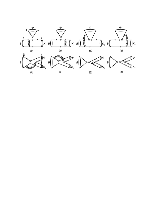
Figure 1: Typical Feynman diagrams contributing to the penguin-dominated $B\to\phi K_{1}$ decays in the pQCD approach at leading order, in which $K_{1}$ stands for the axial-vector $K_{1}(1270)$ and $K_{1}(1400)$, respectively.

From the effective Hamiltonian (29), there are eight types of diagrams contributing to the $B\to\phi K_{1}$ decays in the pQCD approach at leading order as illustrated in Fig. 1. Analogous to the $B\to\phi K^{*}$ decays Chen:2002pz , we calculate the contributions arising from various operators as shown in Eqs. (31)-(37). Hereafter, for the sake of simplicity, we will use $F$ and $M$ to describe the factorizable and non-factorizable amplitudes induced by the $(V-A)(V-A)$ operators, $F^{P_{1}}$ and $M^{P_{1}}$ to describe the factorizable and non-factorizable amplitudes arising from the $(V-A)(V+A)$ operators, and $F^{P_{2}}$ and $M^{P_{2}}$ to describe the factorizable and non-factorizable amplitudes coming from the $(S-P)(S+P)$ operators that obtained by making Fierz transformation from the $(V-A)(V+A)$ operators, respectively.

For the factorizable emission($fe$) diagrams 1(a) and 1(b), the corresponding Feynman amplitudes with one longitudinal polarization($L$) and two transverse polarizations($N$ and $T$) can be read as follows,

$$F_{fe}^{L} = -8\pi C_{F}m_{B}^{2}\int_{0}^{1}dx_{1}dx_{3}\,\int_{0}^{\infty}b_{1}db_{1}b_{3}db_{3}\,\phi_{B}(x_{1},b_{1})\left\{\left[(1+x_{3})\phi_{3}(x_{3})+r_{3}(1-2x_{3})\right.\right.$$ (38)

$$\left.\left.\times(\phi^{t}_{3}(x_{3})+\phi^{s}_{3}(x_{3}))\right]E_{fe}(t_{a})h_{fe}(x_{1},x_{3},b_{1},b_{3})+2r_{3}\phi^{s}_{3}(x_{3})E_{fe}(t_{b})h_{fe}(x_{3},x_{1},b_{3},b_{1})\right\}\;,$$

$$F_{fe}^{N} = -8\pi C_{F}m_{B}^{2}\int_{0}^{1}dx_{1}dx_{3}\,\int_{0}^{\infty}b_{1}db_{1}b_{3}db_{3}\,\phi_{B}(x_{1},b_{1})r_{2}\left\{[\phi^{T}_{3}(x_{3})+2r_{3}\phi^{v}_{3}(x_{3})+r_{3}x_{3}\right.$$ (39)

$$\left.\times(\phi^{v}_{3}(x_{3})-\phi^{a}_{3}(x_{3}))]E_{fe}(t_{a})h_{fe}(x_{1},x_{3},b_{1},b_{3})+r_{3}[\phi^{v}_{3}(x_{3})+\phi^{a}_{3}(x_{3})]E_{fe}(t_{b})h_{fe}(x_{3},x_{1},b_{3},b_{1})\right\}\;,$$

$$F_{fe}^{T} = -16\pi C_{F}m_{B}^{2}\int_{0}^{1}dx_{1}dx_{3}\,\int_{0}^{\infty}b_{1}db_{1}b_{3}db_{3}\,\phi_{B}(x_{1},b_{1})r_{2}\left\{[\phi^{T}_{3}(x_{3})+2r_{3}\phi^{a}_{3}(x_{3})-r_{3}x_{3}\right.$$ (40)

$$\left.\times(\phi^{v}_{3}(x_{3})-\phi^{a}_{3}(x_{3}))]E_{fe}(t_{a})h_{fe}(x_{1},x_{3},b_{1},b_{3})+r_{3}[\phi^{v}_{3}(x_{3})+\phi^{a}_{3}(x_{3})]E_{fe}(t_{b})h_{fe}(x_{3},x_{1},b_{3},b_{1})\right\}\;;$$

where $\phi_{3}$ denotes the distribution amplitude of the axial-vector state $K_{1A}$ or $K_{1B}$ and $C_{F}=4/3$ is a color factor. The hard functions $h_{i}$, the running hard scales $t_{i}$ and the convolution functions $E_{i}(t)$ can be referred to Ref. Chen:2002pz .

Since only the vector part of $(V+A)$ current contributes to the vector meson production, $\langle A|V-A|B\rangle\langle\phi|V+A|0\rangle=\langle A|V-A|B\rangle\langle\phi|V-A|0\rangle,$ that is

$$F_{fe}^{P_{1}}=F_{fe}\;.$$ (41)

For the non-factorizable emission($nfe$) diagrams 1(c) and 1(d), the corresponding Feynman amplitudes are

$$M_{nfe}^{L} = -\frac{16\sqrt{6}}{3}\pi C_{F}m_{B}^{2}\int_{0}^{1}dx_{1}dx_{2}\,dx_{3}\,\int_{0}^{\infty}b_{1}db_{1}b_{2}db_{2}\,\phi_{B}(x_{1},b_{1})\phi_{2}(x_{2})\left\{\left[(1-x_{2})\phi_{3}(x_{3})\right.\right.$$ (42)

$$\left.+r_{3}x_{3}(\phi^{t}_{3}(x_{3})-\phi^{s}_{3}(x_{3}))\right]E_{nfe}(t_{c})h_{nfe}^{c}(x_{1},x_{2},x_{3},b_{1},b_{2})-\left[(x_{2}+x_{3})\phi_{3}(x_{3})\right.$$

$$\left.\left.-r_{3}x_{3}(\phi^{t}_{3}(x_{3})+\phi^{s}_{3}(x_{3}))\right]E_{nfe}(t_{d})h_{nfe}^{d}(x_{1},x_{2},x_{3},b_{1},b_{2})\right\}\;,$$

in which $\phi_{2}$ stands for the distribution amplitude of $\phi$ meson.

$$M_{nfe}^{N} = \frac{16\sqrt{6}}{3}\pi C_{F}m_{B}^{2}\int_{0}^{1}dx_{1}dx_{2}\,dx_{3}\,\int_{0}^{\infty}b_{1}db_{1}b_{2}db_{2}\,\phi_{B}(x_{1},b_{1})r_{2}\left\{(1-x_{2})(\phi^{v}_{2}(x_{2})+\phi^{a}_{2}(x_{2}))\right.$$ (43)

$$\left.\times\phi^{T}_{3}(x_{3})h_{nfe}^{c}(x_{1},x_{2},x_{3},b_{1},b_{2})E_{nfe}(t_{c})+\left[x_{2}(\phi^{v}_{2}(x_{2})+\phi^{a}_{2}(x_{2}))\phi^{T}_{3}(x_{3})\right.\right.$$

$$\left.\left.-2r_{3}(x_{2}+x_{3})(\phi^{v}_{2}(x_{2})\phi^{v}_{3}(x_{3})+\phi^{a}_{2}(x_{2})\phi^{a}_{3}(x_{3}))\right]E_{nfe}(t_{d})h_{nfe}^{d}(x_{1},x_{2},x_{3},b_{1},b_{2})\right\}\;,$$

$$M_{nfe}^{T} = -\frac{32\sqrt{6}}{3}\pi C_{F}m_{B}^{2}\int_{0}^{1}dx_{1}dx_{2}\,dx_{3}\,\int_{0}^{\infty}b_{1}db_{1}b_{2}db_{2}\,\phi_{B}(x_{1},b_{1})r_{2}\left\{(1-x_{2})(\phi^{v}_{2}(x_{2})+\phi^{a}_{2}(x_{2}))\right.$$ (44)

$$\left.\times\phi^{T}_{3}(x_{3})h_{nfe}^{c}(x_{1},x_{2},x_{3},b_{1},b_{2})E_{nfe}(t_{c})+\left[x_{2}(\phi^{v}_{2}(x_{2})+\phi^{a}_{2}(x_{2}))\phi^{T}_{3}(x_{3})\right.\right.$$

$$\left.\left.-2r_{3}(x_{2}+x_{3})(\phi^{v}_{2}(x_{2})\phi^{a}_{3}(x_{3})+\phi^{a}_{2}(x_{2})\phi^{v}_{3}(x_{3}))\right]E_{nfe}(t_{d})h_{nfe}^{d}(x_{1},x_{2},x_{3},b_{1},b_{2})\right\}\;.$$

$$M_{nfe}^{P_{1},L} = -\frac{16\sqrt{6}}{3}\pi C_{F}m_{B}^{2}\int_{0}^{1}dx_{1}dx_{2}\,dx_{3}\,\int_{0}^{\infty}b_{1}db_{1}b_{2}db_{2}\,\phi_{B}(x_{1},b_{1})r_{2}\left\{\left[(1-x_{2})(\phi^{t}_{2}(x_{2})+\phi^{s}_{2}(x_{2}))\right.\right.$$ (45)

$$\times\left.\phi_{3}(x_{3})-r_{3}(1-x_{2})(\phi^{t}_{2}(x_{2})+\phi^{s}_{2}(x_{2}))(\phi^{t}_{3}(x_{3})-\phi^{s}_{3}(x_{3}))-r_{3}x_{3}(\phi^{t}_{2}(x_{2})-\phi^{s}_{2}(x_{2}))\right.$$

$$\left.\times(\phi^{t}_{3}(x_{3})+\phi^{s}_{3}(x_{3}))\right]E_{nfe}(t_{c})h_{nfe}^{c}(x_{1},x_{2},x_{3},b_{1},b_{2})+\left[x_{2}(\phi^{t}_{2}(x_{2})-\phi^{s}_{2}(x_{2}))\phi_{3}(x_{3})\right.$$

$$\left.\left.-r_{3}x_{2}(\phi^{t}_{2}(x_{2})-\phi^{s}_{2}(x_{2}))(\phi^{t}_{3}(x_{3})-\phi^{s}_{3}(x_{3}))-r_{3}x_{3}(\phi^{t}_{2}(x_{2})+\phi^{s}_{2}(x_{2}))(\phi^{t}_{3}(x_{3})+\phi^{s}_{3}(x_{3}))\right]\right.$$

$$\left.\times E_{nfe}(t_{d})h_{nfe}^{d}(x_{1},x_{2},x_{3},b_{1},b_{2})\right\}\;,$$

$$M_{nfe}^{P_{1},N} = -\frac{16\sqrt{6}}{3}\pi C_{F}m_{B}^{2}\int_{0}^{1}dx_{1}dx_{2}\,dx_{3}\,\int_{0}^{\infty}b_{1}db_{1}b_{2}db_{2}\,\phi_{B}(x_{1},b_{1})r_{3}x_{3}\phi^{T}_{2}(x_{2})(\phi^{v}_{3}(x_{3})-\phi^{a}_{3}(x_{3}))$$ (46)

$$\times\left\{E_{nfe}(t_{c})h_{nfe}^{c}(x_{1},x_{2},x_{3},b_{1},b_{2})+E_{nfe}(t_{d})h_{nfe}^{d}(x_{1},x_{2},x_{3},b_{1},b_{2})\right\}\;,$$

$$M_{nfe}^{P_{1},T} = 2M_{nfe}^{P_{1},N}\;,$$ (47)

$$M_{nfe}^{P_{2},L} = -\frac{16\sqrt{6}}{3}\pi C_{F}m_{B}^{2}\int_{0}^{1}dx_{1}dx_{2}\,dx_{3}\,\int_{0}^{\infty}b_{1}db_{1}b_{2}db_{2}\,\phi_{B}(x_{1},b_{1})\phi_{2}(x_{2})\left\{\left[(1-x_{2}+x_{3})\phi_{3}(x_{3})\right.\right.$$ (48)

$$\left.\left.-r_{3}x_{3}(\phi^{t}_{3}(x_{3})+\phi^{s}_{3}(x_{3}))\right]E_{e}(t_{c})h_{nfe}^{c}(x_{1},x_{2},x_{3},b_{1},b_{2})-h_{nfe}^{d}(x_{1},x_{2},x_{3},b_{1},b_{2})E_{nfe}(t_{d})\right.$$

$$\times\left[x_{2}\phi_{3}(x_{3})+r_{3}x_{3}(\phi^{t}_{3}(x_{3})-\phi^{s}_{3}(x_{3}))\right]\left.\right\}\;,$$

$$M_{nfe}^{P_{2},N} = \frac{16\sqrt{6}}{3}\pi C_{F}m_{B}^{2}\int_{0}^{1}dx_{1}dx_{2}\,dx_{3}\,\int_{0}^{\infty}b_{1}db_{1}b_{2}db_{2}\,\phi_{B}(x_{1},b_{1})r_{2}\left\{\left[(1-x_{2})(\phi^{v}_{2}(x_{2})-\phi^{a}_{2}(x_{2}))\right.\right.$$ (49)

$$\left.\left.\times\phi^{T}_{3}(x_{3})-2r_{3}(1-x_{2}+x_{3})(\phi^{v}_{2}(x_{2})\phi^{v}_{3}(x_{3})-\phi^{a}_{2}(x_{2})\phi^{a}_{3}(x_{3}))\right]h_{nfe}^{c}(x_{1},x_{2},x_{3},b_{1},b_{2})\right.$$

$$\left.\times E_{nfe}(t_{c})+x_{2}(\phi^{v}_{2}(x_{2})-\phi^{a}_{2}(x_{2}))\phi^{T}_{3}(x_{3})E_{nfe}(t_{d})h_{nfe}^{d}(x_{1},x_{2},x_{3},b_{1},b_{2})\right\}\;,$$

$$M_{nfe}^{P_{2},T} = \frac{32\sqrt{6}}{3}\pi C_{F}m_{B}^{2}\int_{0}^{1}dx_{1}dx_{2}\,dx_{3}\,\int_{0}^{\infty}b_{1}db_{1}b_{2}db_{2}\,\phi_{B}(x_{1},b_{1})r_{2}\left\{\left[(1-x_{2})(\phi^{v}_{2}(x_{2})-\phi^{a}_{2}(x_{2}))\right.\right.$$ (50)

$$\left.\left.\times\phi^{T}_{3}(x_{3})-2r_{3}(1-x_{2}+x_{3})(\phi^{v}_{2}(x_{2})\phi^{a}_{3}(x_{3})-\phi^{a}_{2}(x_{2})\phi^{v}_{3}(x_{3}))\right]h_{nfe}^{c}(x_{1},x_{2},x_{3},b_{1},b_{2})\right.$$

$$\left.\times E_{nfe}(t_{c})+x_{2}(\phi^{v}_{2}(x_{2})-\phi^{a}_{2}(x_{2}))\phi^{T}_{3}(x_{3})E_{nfe}(t_{d})h_{nfe}^{d}(x_{1},x_{2},x_{3},b_{1},b_{2})\right\}\;,$$

For the non-factorizable annihilation($nfa$) diagrams 1(e) and 1(f), we have

$$M_{nfa}^{L} = -\frac{16\sqrt{6}}{3}\pi C_{F}m_{B}^{2}\int_{0}^{1}dx_{1}dx_{2}\,dx_{3}\,\int_{0}^{\infty}b_{1}db_{1}b_{2}db_{2}\,\phi_{B}(x_{1},b_{1})\left\{\left[(1-x_{3})\phi_{2}(x_{2})\phi_{3}(x_{3})\right.\right.$$ (51)

$$\left.\left.+r_{2}r_{3}\left((1+x_{2}-x_{3})(\phi^{s}_{2}(x_{2})\phi^{s}_{3}(x_{3})-\phi^{t}_{2}(x_{2})\phi^{t}_{3}(x_{3}))-(1-x_{2}-x_{3})(\phi^{s}_{2}(x_{2})\phi^{t}_{3}(x_{3})\right.\right.\right.$$

$$\left.\left.\left.-\phi^{t}_{2}(x_{2})\phi^{s}_{3}(x_{3}))\right)\right]E_{nfa}(t_{e})h_{nfa}^{e}(x_{1},x_{2},x_{3},b_{1},b_{2})-\left[x_{2}\phi_{2}(x_{2})\phi_{3}(x_{3})+2r_{2}r_{3}(\phi^{t}_{2}(x_{2})\right.\right.$$

$$\left.\left.\times\phi^{t}_{3}(x_{3})+\phi^{s}_{2}(x_{2})\phi^{s}_{3}(x_{3}))-r_{2}r_{3}(1+x_{2}-x_{3})(\phi^{t}_{2}(x_{2})\phi^{t}_{3}(x_{3})-\phi^{s}_{2}(x_{2})\phi^{s}_{3}(x_{3}))+r_{2}r_{3}\right.\right.$$

$$\left.\left.\times(1-x_{2}-x_{3})(\phi^{s}_{2}(x_{2})\phi^{t}_{3}(x_{3})-\phi^{t}_{2}(x_{2})\phi^{s}_{3}(x_{3}))\right]E_{nfa}(t_{f})h_{nfa}^{f}(x_{1},x_{2},x_{3},b_{1},b_{2})\right\}\;,$$

$$M_{nfa}^{N} = \frac{32\sqrt{6}}{3}\pi C_{F}m_{B}^{2}\int_{0}^{1}dx_{1}dx_{2}\,dx_{3}\,\int_{0}^{\infty}b_{1}db_{1}b_{2}db_{2}\,\phi_{B}(x_{1},b_{1})r_{2}r_{3}$$ (52)

$$\times\left[\phi^{v}_{2}(x_{2})\phi^{v}_{3}(x_{3})+\phi^{a}_{2}(x_{2})\phi^{a}_{3}(x_{3})\right]E_{nfa}(t_{f})h_{nfa}^{f}(x_{1},x_{2},x_{3},b_{1},b_{2})\;,$$

$$M_{nfa}^{T} = \frac{64\sqrt{6}}{3}\pi C_{F}m_{B}^{2}\int_{0}^{1}dx_{1}dx_{2}\,dx_{3}\,\int_{0}^{\infty}b_{1}db_{1}b_{2}db_{2}\,\phi_{B}(x_{1},b_{1})r_{2}r_{3}$$ (53)

$$\times\left[\phi^{v}_{2}(x_{2})\phi^{a}_{3}(x_{3})+\phi^{a}_{2}(x_{2})\phi^{v}_{3}(x_{3})\right]E_{nfa}(t_{f})h_{nfa}^{f}(x_{1},x_{2},x_{3},b_{1},b_{2})\;.$$

$$M_{nfa}^{P_{1},L} = -\frac{16\sqrt{6}}{3}\pi C_{F}m_{B}^{2}\int_{0}^{1}dx_{1}dx_{2}\,dx_{3}\,\int_{0}^{\infty}b_{1}db_{1}b_{2}db_{2}\,\phi_{B}(x_{1},b_{1})\left\{\left[r_{3}(1-x_{3})(\phi^{s}_{3}(x_{3})-\phi^{t}_{3}(x_{3}))\right.\right.$$ (54)

$$\left.\left.\times\phi_{2}(x_{2})+r_{2}x_{2}(\phi^{t}_{2}(x_{2})+\phi^{s}_{2}(x_{2}))\phi_{3}(x_{3})\right]E_{nfa}(t_{e})h_{nfa}^{e}(x_{1},x_{2},x_{3},b_{1},b_{2})-\left[r_{2}(2-x_{2})\phi_{3}(x_{3})\right.\right.$$

$$\left.\left.\times(\phi^{t}_{2}(x_{2})+\phi^{s}_{2}(x_{2}))-r_{3}(1+x_{3})\phi_{2}(x_{2})(\phi^{s}_{3}(x_{3})-\phi^{t}_{3}(x_{3}))\right]E_{nfa}(t_{f})h_{nfa}^{f}(x_{1},x_{2},x_{3},b_{1},b_{2})\right\}\;,$$

$$M_{nfa}^{P_{1},N} = -\frac{16\sqrt{6}}{3}\pi C_{F}m_{B}^{2}\int_{0}^{1}dx_{1}dx_{2}\,dx_{3}\,\int_{0}^{\infty}b_{1}db_{1}b_{2}db_{2}\,\phi_{B}(x_{1},b_{1})\left\{\left[r_{2}x_{2}(\phi^{v}_{2}(x_{2})+\phi^{a}_{2}(x_{2}))\phi^{T}_{3}(x_{3})\right.\right.$$ (55)

$$\left.\left.-r_{3}(1-x_{3})\phi^{T}_{2}(x_{2})(\phi^{a}_{3}(x_{3})-\phi^{v}_{3}(x_{3}))\right]E_{nfa}(t_{e})h_{nfa}^{e}(x_{1},x_{2},x_{3},b_{1},b_{2})+\left[r_{2}(2-x_{2})\phi^{T}_{3}(x_{3})\right.\right.$$

$$\left.\left.\times(\phi^{v}_{2}(x_{2})+\phi^{a}_{2}(x_{2}))-r_{3}(1+x_{3})\phi^{T}_{2}(x_{2})(\phi^{a}_{3}(x_{3})-\phi^{v}_{3}(x_{3}))\right]E_{nfa}(t_{f})h_{nfa}^{f}(x_{1},x_{2},x_{3},b_{1},b_{2})\right\}\;,$$

$$M_{nfa}^{P_{1},T} = 2M_{nfa}^{P_{1},N}\;,$$ (56)

For the factorizable annihilation($fa$) diagrams 1(g) and 1(h), the contributions are

$$F_{fa}^{L} = -8\pi C_{F}m_{B}^{2}\int_{0}^{1}dx_{2}dx_{3}\,\int_{0}^{\infty}b_{2}db_{2}b_{3}db_{3}\,\left\{\left[x_{2}\phi_{2}(x_{2})\phi_{3}(x_{3})+2r_{3}r_{3}\phi^{s}_{3}(x_{3})((1+x_{2})\phi^{s}_{2}(x_{2})\right.\right.$$ (57)

$$\left.\left.-(1-x_{2})\phi^{t}_{2}(x_{2}))\right]E_{fa}(t_{g})h_{fa}(x_{2},1-x_{3},b_{2},b_{3})-\left[(1-x_{3})\phi_{2}(x_{2})\phi_{3}(x_{3})+2r_{2}r_{3}\phi^{s}_{2}(x_{2})\right.\right.$$

$$\left.\left.\times(x_{3}\phi^{t}_{3}(x_{3})+(2-x_{3})\phi^{s}_{3}(x_{3}))\right]E_{fa}(t_{h})h_{fa}(1-x_{3},x_{2},b_{3},b_{2})\right\}\;,$$

$$F_{fa}^{N} = -8\pi C_{F}m_{B}^{2}\int_{0}^{1}dx_{2}dx_{3}\,\int_{0}^{\infty}b_{2}db_{2}b_{3}db_{3}\,r_{2}r_{3}\left\{E_{fa}(t_{g})\left[(1+x_{2})(\phi^{v}_{2}(x_{2})\phi^{v}_{3}(x_{3})+\phi^{a}_{2}(x_{2})\phi^{a}_{3}(x_{3}))\right.\right.$$ (58)

$$\left.\left.-(1-x_{2})(\phi^{v}_{2}(x_{2})\phi^{a}_{3}(x_{3})+\phi^{a}_{2}(x_{2})\phi^{v}_{3}(x_{3}))\right]h_{fa}(x_{2},1-x_{3},b_{2},b_{3})-\left[(2-x_{3})(\phi^{v}_{2}(x_{2})\phi^{v}_{3}(x_{3})\right.\right.$$

$$\left.\left.+\phi^{a}_{2}(x_{2})\phi^{a}_{3}(x_{3}))+x_{3}(\phi^{v}_{2}(x_{2})\phi^{a}_{3}(x_{3})+\phi^{a}_{2}(x_{2})\phi^{v}_{3}(x_{3}))\right]E_{fa}(t_{h})h_{fa}(1-x_{3},x_{2},b_{3},b_{2})\right\}\;,$$

$$F_{fa}^{T} = -16\pi C_{F}m_{B}^{2}\int_{0}^{1}dx_{2}dx_{3}\,\int_{0}^{\infty}b_{2}db_{2}b_{3}db_{3}\,r_{2}r_{3}\left\{E_{fa}(t_{g})\left[(1+x_{2})(\phi^{v}_{2}(x_{2})\phi^{a}_{3}(x_{3})+\phi^{a}_{2}(x_{2})\phi^{v}_{3}(x_{3}))\right.\right.$$ (59)

$$\left.\left.-(1-x_{2})(\phi^{v}_{2}(x_{2})\phi^{v}_{3}(x_{3})+\phi^{a}_{2}(x_{2})\phi^{a}_{3}(x_{3}))\right]h_{fa}(x_{2},1-x_{3},b_{2},b_{3})+\left[x_{3}(\phi^{v}_{2}(x_{2})\phi^{v}_{3}(x_{3})\right.\right.$$

$$\left.\left.+\phi^{a}_{2}(x_{2})\phi^{a}_{3}(x_{3}))+(2-x_{3})(\phi^{v}_{2}(x_{2})\phi^{a}_{3}(x_{3})+\phi^{a}_{2}(x_{2})\phi^{v}_{3}(x_{3}))\right]E_{fa}(t_{h})h_{fa}(1-x_{3},x_{2},b_{3},b_{2})\right\}\;;$$

$$F_{fa}^{P_{2},L} = -16\pi C_{F}m_{B}^{2}\int_{0}^{1}dx_{2}dx_{3}\,\int_{0}^{\infty}b_{2}db_{2}b_{3}db_{3}\,\left\{\left[2r_{3}\phi_{2}(x_{2})\phi^{s}_{3}(x_{3})-r_{2}{x_{2}}(\phi^{t}_{2}(x_{2})-\phi^{s}_{2}(x_{2}))\right.\right.$$ (60)

$$\left.\left.\times\phi_{3}(x_{3})\right]h_{fa}(x_{2},1-x_{3},b_{2},b_{3})E_{fa}(t_{g})+\left[2r_{2}\phi^{s}_{2}(x_{2})\phi_{3}(x_{3})+r_{3}(1-x_{3})\phi_{2}(x_{2})\right.\right.$$

$$\left.\left.\times(\phi^{t}_{3}(x_{3})+\phi^{s}_{3}(x_{3}))\right]E_{fa}(t_{h})h_{fa}(1-x_{3},x_{2},b_{3},b_{2})\right\}\;,$$

$$F_{fa}^{P_{2},N} = -16\pi C_{F}m_{B}^{2}\int_{0}^{1}dx_{2}dx_{3}\,\int_{0}^{\infty}b_{2}db_{2}b_{3}db_{3}\,\left\{r_{3}\phi^{T}_{2}(x_{2})(\phi^{a}_{3}(x_{3})-\phi^{v}_{3}(x_{3}))h_{fa}(x_{2},1-x_{3},b_{2},b_{3})\right.$$ (61)

$$\left.\times E_{fa}(t_{g})+r_{2}(\phi^{v}_{2}(x_{2})+\phi^{a}_{2}(x_{2}))\phi^{T}_{3}(x_{3})E_{fa}(t_{h})h_{fa}(1-x_{3},x_{2},b_{3},b_{2})\right\}\;,$$

$$F_{fa}^{P_{2},T} = 2F_{fa}^{P_{2},N};$$ (62)

Before we put the things together to write down the decay amplitudes for the considered $B\to\phi K_{1}$ modes, it is essential to give a brief discussion about the ”$K_{1}(1270)-K_{1}(1400)$” mixing. The physical mass eigenstates $K_{1}(1270)$ and $K_{1}(1400)$ are believed to be the mixtures of the $K_{1A}(^{3}P_{1})$ and $K_{1B}(^{1}P_{1})$ states with the mixing angle $\theta_{K_{1}}$ due to the mass difference of the strange and non-strange light quarks. Following the common convention, their relations can be written as Beringer:1900zz

$$\left(\begin{array}[]{c}|K_{1}(1270)\rangle\\ |K_{1}(1400)\rangle\\ \end{array}\right) = \left(\begin{array}[]{cc}\sin{\theta_{K_{1}}}&\hskip 7.96674pt\cos{\theta_{K_{1}}}\\ \cos{\theta_{K_{1}}}&-\sin\theta_{K_{1}}\end{array}\right)\left(\begin{array}[]{c}|K_{1A}\rangle\\ |K_{1B}\rangle\\ \end{array}\right)\;,$$ (69)

There exist several estimations on the mixing angle $\theta_{K_{1}}$ in the literature Suzuki:1993yc ; Burakovsky:1997dd ; Cheng:2003bn ; Hatanaka:2008xj ; Cheng:2011pb ; Divotgey:2013jba . Various phenomenological studies indicate that the $K_{1A}-K_{1B}$ mixing angle $\theta_{K_{1}}$ is around either $33^{\circ}$ or $58^{\circ}$ but with a twofold ambiguity. The sign ambiguity for $\theta_{K_{1}}$ is due to the fact that one can add arbitrary phases to $|K_{1A}\rangle$ and $|K_{1B}\rangle$. As discussed in Ref. Cheng:2011pb and many early publications, the sign ambiguity of $\theta_{K_{1}}$ can be removed by fixing the relative sign of the decay constants of $|K_{1A}\rangle$ and $|K_{1B}\rangle$. We shall choose the convention of decay constants in such a way that $\theta_{K_{1}}$ is always positive. It is noted that the sign of the mixing angle $\theta_{K_{1}}$ is positive for the mixing of particle states $K_{1A}$ and $K_{1B}$ in this work, which corresponds to the negative sign of $\theta_{K_{1}}$ between the mixing of antiparticle states $\bar{K}_{1A}$ and $\bar{K}_{1B}$ in the literature Hatanaka:2008xj . The underlying reason is that, as discussed in Ref. Blundell:1996as , the spin-orbit portion $<H_{q\bar{q}}^{SO-}>$ in the constituent quark model Hamiltonian causes the mixing between $K_{1A}(^{3}P_{1})$ and $K_{1B}(^{1}P_{1})$ states, changes the sign when the antiquark instead of the quark is the heavier strange, then further leads to a mixing angle of opposite sign when the ${}^{3}P_{1}-^{1}P_{1}$ Hamiltonian is diagonalized. In other words, if we have a angle of $-33^{\circ}$ for the mixing of antiparticles $K_{1}(1270)^{-}$ and $K_{1}(1400)^{-}$, we must use $+33^{\circ}$ for that of the particles $K_{1}(1270)^{+}$ and $K_{1}(1400)^{+}$. For the value of mixing angle $\theta_{K_{1}}$, we shall adopt both $33^{\circ}$ and $58^{\circ}$ in the numerical evaluations, which is because almost no any precise measurements on $\theta_{K_{1}}$ exist to date and one can identify the more favored value of the mixing angle in the relevant $B$ meson decays, though Refs. Hatanaka:2008xj ; Cheng:2011pb ; Cheng:2013cwa suggested that the smaller angle $\theta_{K_{1}}\sim 33^{\circ}$ is much more favored than $58^{\circ}$.

Thus, by combining various contributions from different diagrams as presented in Eqs. (38)-(62) and the mixing pattern in Eq. (69), the total decay amplitudes for the penguin dominated $B\to\phi K_{1}(1270)$ can be written as

$${\cal M}_{h}(B^{+}\to\phi K_{1}(1270)^{+}) = A_{h}(B^{+}\to\phi K_{1A}^{+}){\rm{\sin}}\theta_{K_{1}}+A_{h}(B^{+}\to\phi K_{1B}^{+}){\rm{\cos}}\theta_{K_{1}}$$ (70)

$$= -\lambda_{t}f_{\phi}\left(a_{3}+a_{4}+a_{5}-\frac{1}{2}(a_{7}+a_{9}+a_{10})\right)(F_{fe;K_{1A}}^{h}{\rm{\sin}}\theta_{K_{1}}+F_{fe;K_{1B}}^{h}{\rm{\cos}}\theta_{K_{1}})$$

$$-\lambda_{t}\biggl{\{}(M_{nfe;K_{1A}}^{h}{\rm{\sin}}\theta_{K_{1}}+M_{nfe;K_{1B}}^{h}{\rm{\cos}}\theta_{K_{1}})(C_{3}+C_{4}-\frac{1}{2}(C_{9}+C_{10}))$$

$$+(C_{5}-\frac{1}{2}C_{7})(M_{nfe;K_{1A}}^{P_{1};h}{\rm{\sin}}\theta_{K_{1}}+M_{nfe;K_{1B}}^{P_{1};h}{\rm{\cos}}\theta_{K_{1}})+(C_{6}-\frac{1}{2}C_{8})(M_{nfe;K_{1A}}^{P_{2};h}$$

$$\cdot{\rm{\sin}}\theta_{K_{1}}+{\rm{\cos}}\theta_{K_{1}}M_{nfe;K_{1B}}^{P_{2};h})\biggr{\}}+\lambda_{u}C_{1}(M_{nfa;K_{1A}}^{h}{\rm{\sin}}\theta_{K_{1}}+M_{nfa;K_{1B}}^{h}{\rm{\cos}}\theta_{K_{1}})$$

$$-\lambda_{t}\biggl{\{}(C_{3}+C_{9})(M_{nfa;K_{1A}}^{h}{\rm{\sin}}\theta_{K_{1}}+M_{nfa;K_{1B}}^{h}{\rm{\cos}}\theta_{K_{1}})+(C_{5}+C_{7})$$

$$\cdot(M_{nfa;K_{1A}}^{P_{1};h}{\rm{\sin}}\theta_{K_{1}}+M_{nfa;K_{1B}}^{P_{1};h}{\rm{\cos}}\theta_{K_{1}})\biggr{\}}+\lambda_{u}a_{1}(F_{fa;K_{1A}}^{h}{\rm{\sin}}\theta_{K_{1}}+F_{fa;K_{1B}}^{h}$$

$$\cdot{\rm{\cos}}\theta_{K_{1}})f_{B}-\lambda_{t}\biggl{\{}(a_{4}+a_{10})(F_{fa;K_{1A}}^{h}{\rm{\sin}}\theta_{K_{1}}+F_{fa;K_{1B}}^{h}{\rm{\cos}}\theta_{K_{1}})+(a_{6}+a_{8})$$

$$\cdot(F_{fa;K_{1A}}^{P_{2};h}{\rm{\sin}}\theta_{K_{1}}+F_{fa;K_{1B}}^{P_{2};h}{\rm{\cos}}\theta_{K_{1}})\biggr{\}}f_{B};$$

$${\cal M}_{h}(B^{0}\to\phi K_{1}(1270)^{0}) = A_{h}(B^{0}\to\phi K_{1A}^{0}){\rm{\sin}}\theta_{K_{1}}+A_{h}(B^{0}\to\phi K_{1B}^{0}){\rm{\cos}}\theta_{K_{1}}$$ (71)

$$= -\lambda_{t}f_{\phi}\left(a_{3}+a_{4}+a_{5}-\frac{1}{2}(a_{7}+a_{9}+a_{10})\right)(F_{fe;K_{1A}}^{h}{\rm{\sin}}\theta_{K_{1}}+F_{fe;K_{1B}}^{h}{\rm{\cos}}\theta_{K_{1}})$$

$$-\lambda_{t}\biggl{\{}(M_{nfe;K_{1A}}^{h}{\rm{\sin}}\theta_{K_{1}}+M_{nfe;K_{1B}}^{h}{\rm{\cos}}\theta_{K_{1}})(C_{3}+C_{4}-\frac{1}{2}(C_{9}+C_{10}))$$

$$+(C_{5}-\frac{1}{2}C_{7})(M_{nfe;K_{1A}}^{P_{1};h}{\rm{\sin}}\theta_{K_{1}}+M_{nfe;K_{1B}}^{P_{1};h}{\rm{\cos}}\theta_{K_{1}})+(C_{6}-\frac{1}{2}C_{8})(M_{nfe;K_{1A}}^{P_{2};h}$$

$$\cdot{\rm{\sin}}\theta_{K_{1}}+{\rm{\cos}}\theta_{K_{1}}M_{nfe;K_{1B}}^{P_{2};h})\biggr{\}}-\lambda_{t}\biggl{\{}(C_{3}-\frac{1}{2}C_{9})(M_{nfa;K_{1A}}^{h}{\rm{\sin}}\theta_{K_{1}}+M_{nfa;K_{1B}}^{h}$$

$$\cdot{\rm{\cos}}\theta_{K_{1}})+(C_{5}-\frac{1}{2}C_{7})(M_{nfa;K_{1A}}^{P_{1};h}{\rm{\sin}}\theta_{K_{1}}+M_{nfa;K_{1B}}^{P_{1};h}{\rm{\cos}}\theta_{K_{1}})\biggr{\}}-\lambda_{t}f_{B}\biggl{\{}(a_{4}-\frac{1}{2}a_{10})$$

$$\cdot(F_{fa;K_{1A}}^{h}{\rm{\sin}}\theta_{K_{1}}+F_{fa;K_{1B}}^{h}{\rm{\cos}}\theta_{K_{1}})+(a_{6}-\frac{1}{2}a_{8})(F_{fa;K_{1A}}^{P_{2};h}{\rm{\sin}}\theta_{K_{1}}+F_{fa;K_{1B}}^{P_{2};h}{\rm{\cos}}\theta_{K_{1}})\biggr{\}};$$

where $\lambda_{u}=V^{*}_{ub}V_{us},\lambda_{t}=V^{*}_{tb}V_{ts}$ and ${\cal M}_{h}$ in the above equations denotes the different helicity amplitudes ${\cal M}_{L}$, ${\cal M}_{N}$, and ${\cal M}_{T}$, respectively. And $a_{i}$ is the standard combination of the Wilson coefficients $C_{i}$ defined as follows:

$$a_{1} = C_{2}+\frac{C_{1}}{3};\quad a_{i}=C_{i}+C_{i\pm 1}/3,\quad i=3-10.$$ (72)

where $C_{2}\sim 1$ is the largest one among all Wilson coefficients and the upper (lower) sign applies, when $i$ is odd (even). When we make the replacements with ${\rm{\sin}}\theta_{K_{1}}\to{\rm{\cos}}\theta_{K_{1}},{\rm{\cos}}\theta_{K_{1}}\to-{\rm{\sin}}\theta_{K_{1}}$ in Eqs.(70) and (71), respectively, the total decay amplitudes for the $B\to\phi K_{1}(1400)$ decays can be obtained straightforwardly.

III Numerical Results and Discussions

In this section, we will present the pQCD predictions on the CP-averaged branching ratios, the polarization fractions, the relative phases and the CP-violating asymmetries for those four $B\to\phi K_{1}$ decay modes. In numerical calculations, central values of the input parameters will be used implicitly unless otherwise stated. The relevant QCD scale (GeV), masses (GeV), and $B$ meson lifetime(ps) are the following  Keum:2000ph ; Keum:2000wi ; Lu:2000em ; Yang:2007zt ; Beringer:1900zz

$$\Lambda_{\overline{\mathrm{MS}}}^{(f=4)} = 0.250\;,\quad m_{W}=80.41\;,\quad m_{B}=5.2794\;,\quad m_{b}=4.8\;,\quad m_{\phi}=1.02\;;$$

$$f_{K_{1A}} = 0.250\;,\quad f_{K_{1B}}=0.190\;,\quad m_{K_{1A}}=1.32\;,\quad m_{K_{1B}}=1.34\;,$$

$$\tau_{B^{+}} = 1.641\;,\quad\tau_{B^{0}}=1.519\;.$$ (73)

For the CKM matrix elements, we adopt the Wolfenstein parametrization and the updated parameters $A=0.811$, $\lambda=0.22535$, $\bar{\rho}=0.131^{+0.026}_{-0.013}$, and $\bar{\eta}=0.345^{+0.013}_{-0.014}$ Beringer:1900zz .

III.1 CP-averaged branching ratios

For the considered $B\to\phi K_{1}$ decays, the decay rate can be written as

$$\Gamma=\frac{G_{F}^{2}|\bf{P_{c}}|}{16\pi m^{2}_{B}}\sum_{\sigma=L,T}{\cal M}^{(\sigma)\dagger}{\cal M^{(\sigma)}}\;$$ (74)

where $|\bf{P_{c}}|\equiv|\bf{P_{2z}}|=|\bf{P_{3z}}|$ is the momentum of either of the outgoing axial-vector meson or vector meson and ${\cal M^{(\sigma)}}$ can be found in Eqs. (70-71). Using the decay amplitudes obtained in last section, it is straightforward to calculate the CP-averaged branching ratios with uncertainties for the considered decays in the pQCD approach.

Table 1: Theoretical predictions on physical quantities of $B^{+}\to\phi K_{1}(1270)^{+}$ decay obtained in the pQCD approach with the mixing angle $\theta_{K_{1}}\sim 33^{\circ}$ and $58^{\circ}$, respectively. For comparison, we also quote the available experimental measurements Aubert:2008bc and the estimations in the framework of QCD factorization Cheng:2008gxa .

Decay Mode		$B^{+}\to\phi K_{1}(1270)^{+}$
Parameter	Definition	pQCD ($\theta_{K_{1}}\sim 33^{\circ}$)	QCDF ($\theta_{K_{1}}\sim 37^{\circ}$)	pQCD ($\theta_{K_{1}}\sim 58^{\circ}$)	QCDF ($\theta_{K_{1}}\sim 58^{\circ}$)	Experiment
BR($10^{-6}$)	$\Gamma/\Gamma_{\rm total}$	$5.4^{+0.9+0.5+3.3+2.1}_{-0.5-0.5-2.3-1.2}$	$3.8^{+1.9+5.1}_{-1.5-3.1}$	$9.2^{+0.2+1.3+4.4+2.5}_{-0.2-1.2-3.4-1.9}$	$3.4^{+2.2+5.5}_{-1.5-2.8}$	$6.1\pm 1.6\pm 1.1$
$f_{L}$	$|{\cal A}_{L}|^{2}$	$0.47^{+0.11+0.08+0.28+0.01}_{-0.09-0.06-0.30-0.00}$	$0.67^{+0.33}_{-0.64}$	$0.11^{+0.00+0.00+0.11+0.01}_{-0.01-0.02-0.07-0.01}$	$0.31^{+0.69}_{-0.37}$	$0.46^{+0.12+0.06}_{-0.13-0.07}$
$f_{||}$	$|{\cal A}_{||}|^{2}$	$0.30^{+0.06+0.03+0.17+0.00}_{-0.06-0.03-0.19-0.00}$	$-$	$0.45^{+0.01+0.00+0.06+0.00}_{-0.01-0.02-0.11-0.00}$	$-$	$-$
$f_{\perp}$	$|{\cal A}_{\perp}|^{2}$	$0.22^{+0.04+0.05+0.17+0.00}_{-0.04-0.03-0.14-0.00}$	$-$	$0.45^{+0.01+0.00+0.05+0.01}_{-0.01-0.01-0.08-0.02}$	$-$	$-$
$\phi_{||}$(rad)	$\arg\frac{{\cal A}_{||}}{{\cal A}_{L}}$	$2.2^{+0.1+0.0+0.3+0.1}_{-0.1-0.1-0.3-0.1}$	$-$	$3.3^{+0.0+0.1+0.6+0.0}_{-0.0-0.1-0.9-0.1}$	$-$	$-$
$\phi_{\perp}$(rad)	$\arg\frac{{\cal A}_{\perp}}{{\cal A}_{L}}$	$4.4^{+0.0+0.1+0.2+0.0}_{-1.4-0.1-2.4-1.4}$	$-$	$2.6^{+0.0+0.1+0.7+0.0}_{-0.0-0.1-1.0-0.0}$	$-$	$-$
${\cal A}_{CP}^{\rm dir}(10^{-2})$	$\frac{\overline{\Gamma}-\Gamma}{\overline{\Gamma}+\Gamma}$	$-0.7^{+0.5+0.5+3.3+1.2}_{-0.3-0.4-2.6-1.3}$	$-$	$-1.3^{+0.0+0.3+0.9+0.5}_{-0.1-0.2-0.5-0.6}$	$-$	$-15\pm 19\pm 5$
${\cal A}_{CP}^{\rm dir}(L)$	$\frac{\bar{f}_{L}-f_{L}}{\bar{f}_{L}+f_{L}}$	$0.04^{+0.09}_{-0.07}$	$-$	$0.16^{+0.08}_{-0.10}$	$-$	$-$
${\cal A}_{CP}^{\rm dir}(||)$	$\frac{\bar{f}_{||}-f_{||}}{\bar{f}_{||}+f_{||}}$	$-0.33^{+0.12}_{-0.14}$	$-$	$-0.29^{+0.09}_{-0.08}$	$-$	$-$
${\cal A}_{CP}^{\rm dir}(\perp)$	$\frac{\bar{f}_{\perp}-f_{\perp}}{\bar{f}_{\perp}+f_{\perp}}$	$0.33^{+0.11}_{-0.09}$	$-$	$0.22^{+0.05}_{-0.05}$	$-$	$-$

The numerical results of the physical quantities are presented in Tables 1-4, in which the major errors are induced by the uncertainties of the shape parameter $\omega_{b}=0.40\pm 0.04$ GeV for the $B$ meson wave function, of the vector $\phi$ meson decay constants $f_{\phi}=0.231\pm 0.004$ GeV and $f_{\phi}^{T}=0.200\pm 0.010$ GeV and the axial-vector $K_{1A}$ and $K_{1B}$ states decay constants $f_{K_{1A}}=0.250\pm 0.013$ GeV and $f_{K_{1B}}=0.190\pm 0.010$ GeV, and of the Gegenbauer moments $a_{i}^{A,B}(i=0,1,2)$ for the axial-vector $K_{1A}$ and $K_{1B}$ states and $a_{2}$ for the vector $\phi$ meson in both longitudinal and transverse polarizations, respectively. Moreover, in this work, as displayed in the above mentioned Tables, the higher order contributions are also simply investigated by exploring the variation of the hard scale $t_{\rm max}$, i.e., from $0.8t$ to $1.2t$ (not changing $1/b_{i},i=1,2,3$), in the hard kernel, which have been counted into one of the source of theoretical uncertainties(See the last term of errors in the related Tables). Note that the variation of the CKM parameters has tiny or almost no effects to the physical observables of these $B\to\phi K_{1}$ decays in the pQCD approach and thus have been neglected in the relevant numerical results.

Table 2: Same as Table 1 but of $B^{+}\to\phi K_{1}(1400)^{+}$ decay.

Decay Mode		$B^{+}\to\phi K_{1}(1400)^{+}$
Parameter	Definition	pQCD ($\theta_{K_{1}}\sim 33^{\circ}$)	QCDF ($\theta_{K_{1}}\sim 37^{\circ}$)	pQCD ($\theta_{K_{1}}\sim 58^{\circ}$)	QCDF ($\theta_{K_{1}}\sim 58^{\circ}$)	Experiment
BR($10^{-6}$)	$\Gamma/\Gamma_{\rm total}$	$25.1^{+8.5+2.1+10.7+4.4}_{-6.0-2.2-8.9-3.7}$	$11.1^{+8.5+41.1}_{-5.4-11.4}$	$21.4^{+9.3+2.0+7.9+3.9}_{-6.3-1.8-6.7-3.0}$	$11.3^{+7.5+40.2}_{-4.9-11.1}$	$<3.2(0.3\pm 1.6\pm 0.7)(90\%\ {\rm C.L.})$
$f_{L}$	$|{\cal A}_{L}|^{2}$	$0.57^{+0.06+0.03+0.12+0.02}_{-0.06-0.02-0.11-0.02}$	$0.45^{+0.13}_{-0.09}$	$0.74^{+0.04+0.02+0.10+0.02}_{-0.04-0.02-0.09-0.00}$	$0.57^{+0.32}_{-0.22}$	$-$
$f_{||}$	$|{\cal A}_{||}|^{2}$	$0.20^{+0.03+0.01+0.07+0.01}_{-0.03-0.02-0.06-0.01}$	$-$	$0.12^{+0.02+0.00+0.06+0.00}_{-0.02-0.00-0.05-0.01}$	$-$	$-$
$f_{\perp}$	$|{\cal A}_{\perp}|^{2}$	$0.23^{+0.03+0.00+0.05+0.01}_{-0.03-0.02-0.05-0.01}$	$-$	$0.14^{+0.02+0.00+0.04+0.00}_{-0.02-0.02-0.05-0.01}$	$-$	$-$
$\phi_{||}$(rad)	$\arg\frac{{\cal A}_{||}}{{\cal A}_{L}}$	$4.1^{+0.1+0.0+0.2+0.1}_{-0.1-0.0-0.2-0.0}$	$-$	$4.0^{+0.1+0.0+0.2+0.1}_{-0.1-0.0-0.3-0.0}$	$-$	$-$
$\phi_{\perp}$(rad)	$\arg\frac{{\cal A}_{\perp}}{{\cal A}_{L}}$	$3.7^{+0.0+0.0+0.2+0.1}_{-0.0-0.0-0.2-0.1}$	$-$	$3.8^{+0.0+0.0+0.2+0.1}_{-0.0-0.0-0.2-0.1}$	$-$	$-$
${\cal A}_{CP}^{\rm dir}(10^{-2})$	$\frac{\overline{\Gamma}-\Gamma}{\overline{\Gamma}+\Gamma}$	$-1.5^{+0.3+0.1+1.1+0.3}_{-0.4-0.1-1.4-0.3}$	$-$	$-1.3^{+0.2+0.0+1.4+0.5}_{-0.4-0.2-1.6-0.5}$	$-$	$-$
${\cal A}_{CP}^{\rm dir}(L)$	$\frac{\bar{f}_{L}-f_{L}}{\bar{f}_{L}+f_{L}}$	$-0.01^{+0.02}_{-0.02}$	$-$	$-0.01^{+0.01}_{-0.04}$	$-$	$-$
${\cal A}_{CP}^{\rm dir}(||)$	$\frac{\bar{f}_{||}-f_{||}}{\bar{f}_{||}+f_{||}}$	$-0.17^{+0.05}_{-0.03}$	$-$	$-0.08^{+0.05}_{-0.06}$	$-$	$-$
${\cal A}_{CP}^{\rm dir}(\perp)$	$\frac{\bar{f}_{\perp}-f_{\perp}}{\bar{f}_{\perp}+f_{\perp}}$	$0.11^{+0.02}_{-0.04}$	$-$	$0.05^{+0.03}_{-0.06}$	$-$	$-$

Based on the theoretical branching ratios given at leading order in the pQCD approach, some phenomenological remarks on the $B\to\phi K_{1}$ decays are in order:

• From Table 1, one can easily find that the CP-averaged branching ratios of $B^{+}\to\phi K_{1}(1270)^{+}$ decay are

  $$Br(B^{+}\to\phi K_{1}(1270)^{+})_{\rm pQCD} = \left\{\begin{array}[]{ll}5.4^{+4.0}_{-2.7}\times 10^{-6}\;\;\;\;\;\;\;\;{\rm\theta_{K_{1}}\sim 33^{\circ}}&\vspace{0.1cm}\\ 9.2^{+5.2}_{-4.1}\times 10^{-6}\;\;\;\;\;\;\;\;{\rm\theta_{K_{1}}\sim 58^{\circ}}&\\ \end{array}\right.\;,$$ (77)

  where various errors arising from the input parameters have been added in quadrature. It is observed that the former prediction with the smaller angle $33^{\circ}$ is more consistent with the available measurement Aubert:2008bc ,

  $$Br(B^{\pm}\to\phi K_{1}(1270)^{\pm})_{\rm Exp.} = (6.1\pm 1.9)\times 10^{-6}\;,$$ (78)

  where the systematic and statistical errors have also been added in quadrature, although the latter prediction basically agrees with the theoretical values obtained in the framework of QCD factorization and the preliminary data reported by BABAR Collaboration within large errors.

• According to Table 2, the CP-averaged branching ratios of $B^{+}\to\phi K_{1}(1400)^{+}$ decay with two different mixing angles can be read as

  $$Br(B^{+}\to\phi K_{1}(1400)^{+})_{\rm pQCD} = \left\{\begin{array}[]{ll}25.1^{+14.5}_{-11.6}\times 10^{-6}\;\;\;\;\;\;\;\;{\rm\theta_{K_{1}}\sim 33^{\circ}}&\vspace{0.1cm}\\ 21.4^{+13.0}_{-9.8}\times 10^{-6}\;\;\;\;\;\;\;\;{\rm\theta_{K_{1}}\sim 58^{\circ}}&\\ \end{array}\right.\;,$$ (81)

  Here, we have added all the errors in quadrature. Our theoretical predictions are in agreement with that derived in the QCDF approach within large errors and also with the preliminary upper limit Aubert:2008bc

  $$Br(B^{\pm}\to\phi K_{1}(1400)^{\pm})_{\rm Exp.} < 3.2(0.3\pm 1.6\pm 0.7)\times 10^{-6}\;,$$ (82)

  in 2$\sigma$ errors roughly. But, it looks that, unfortunately, the central values significantly exceed the upper limit placed by only BABAR Collaboration. It will be very interesting and probably a challenge for the theorists to further understand the QCD dynamics of these two strange axial-vector mesons and the mixing between $K_{1A}$ and $K_{1B}$ states in depth once the experiments at LHC and/or Super-B confirm the aforementioned much small upper limits of $Br(B^{+}\to\phi K_{1}(1400)^{+})$ in the near future.

• As can be seen in Tables 3 and 4, the CP-averaged branching ratios of $B^{0}\to\phi K_{1}^{0}$ decays with two different mixing angles are also predicted in the pQCD approach,

  $$Br(B^{0}\to\phi K_{1}(1270)^{0})_{\rm pQCD} = \left\{\begin{array}[]{ll}5.1^{+3.5}_{-2.7}\times 10^{-6}\;\;\;\;\;\;\;\;{\rm\theta_{K_{1}}\sim 33^{\circ}}&\vspace{0.1cm}\\ 9.2^{+5.5}_{-4.0}\times 10^{-6}\;\;\;\;\;\;\;\;{\rm\theta_{K_{1}}\sim 58^{\circ}}&\\ \end{array}\right.\;,$$ (85)

  $$Br(B^{0}\to\phi K_{1}(1400)^{0})_{\rm pQCD} = \left\{\begin{array}[]{ll}22.5^{+12.8}_{-10.3}\times 10^{-6}\;\;\;\;\;\;\;\;{\rm\theta_{K_{1}}\sim 33^{\circ}}&\vspace{0.1cm}\\ 18.5^{+11.3}_{-8.8}\times 10^{-6}\;\;\;\;\;\;\;\;{\rm\theta_{K_{1}}\sim 58^{\circ}}&\\ \end{array}\right.\;.$$ (88)

  which are consistent with the predictions in the QCDF approach within large theoretical errors and will be tested in the running LHC and forthcoming Super-B experiments.

• As discussed in Refs. Yang:2007zt ; Cheng:2008gxa , the behavior of the axial-vector ${}^{3}P_{1}$ states is similar to that of the vector mesons, which will consequently result in the branching ratio of $B\to\phi K_{1A}$ analogous to that of $B\to\phi K^{*}$ decays in the pQCD approach. However, from Tables 1-4, it can be clearly observed that the predicted branching ratios of $B\to\phi K_{1}(1270)(B\to\phi K_{1}(1400))$ decays in the pQCD approach are smaller(larger) than those of $B\to\phi K^{*}$ decays Chen:2002pz , which imply the destructive(constructive) effects between $B\to\phi K_{1A}$ and $B\to\phi K_{1B}$ decay amplitudes to $B\to\phi K_{1}(1270)(B\to\phi K_{1}(1400))$ decays. In order to clarify this point more clearly, we present the decay amplitudes of the $B^{+}\to\phi K_{1A}^{+}$ and $B^{+}\to\phi K_{1B}^{+}$ decays numerically for every topology with three polarizations, which can be seen in Table 5.

  Table 3: Same as Table 1 but of $B^{0}\to\phi K_{1}(1270)^{0}$ decay.

  Decay Mode		$B^{0}\to\phi K_{1}(1270)^{0}$
  Parameter	Definition	pQCD ($\theta_{K_{1}}\sim 33^{\circ}$)	QCDF ($\theta_{K_{1}}\sim 37^{\circ}$)	pQCD ($\theta_{K_{1}}\sim 58^{\circ}$)	QCDF ($\theta_{K_{1}}\sim 58^{\circ}$)	Experiment
  BR($10^{-6}$)	$\Gamma/\Gamma_{\rm total}$	$5.1^{+0.7+0.4+2.9+1.8}_{-0.5-0.5-2.3-1.2}$	$3.6^{+1.7+4.8}_{-1.3-2.9}$	$9.2^{+0.2+1.3+4.7+2.5}_{-0.1-1.2-3.4-1.8}$	$3.2^{+2.1+5.2}_{-1.4-2.7}$	$-$
  $f_{L}$	$|{\cal A}_{L}|^{2}$	$0.42^{+0.11+0.06+0.30+0.01}_{-0.09-0.06-0.28-0.00}$	$0.67^{+0.33}_{-0.64}$	$0.11^{+0.00+0.02+0.13+0.01}_{-0.00-0.01-0.06-0.00}$	$0.31^{+0.69}_{-0.31}$	$-$
  $f_{||}$	$|{\cal A}_{||}|^{2}$	$0.35^{+0.05+0.02+0.14+0.00}_{-0.07-0.04-0.20-0.01}$	$-$	$0.45^{+0.01+0.00+0.07+0.01}_{-0.01-0.00-0.11-0.00}$	$-$	$-$
  $f_{\perp}$	$|{\cal A}_{\perp}|^{2}$	$0.24^{+0.03+0.03+0.13+0.00}_{-0.05-0.05-0.17-0.01}$	$-$	$0.44^{+0.01+0.00+0.05+0.01}_{-0.01-0.01-0.07-0.02}$	$-$	$-$
  $\phi_{||}$(rad)	$\arg\frac{{\cal A}_{||}}{{\cal A}_{L}}$	$2.3^{+0.1+0.1+0.4+0.1}_{-0.1-0.1-0.3-0.1}$	$-$	$3.4^{+0.0+0.1+0.5+0.0}_{-0.0-0.1-0.8-0.1}$	$-$	$-$
  $\phi_{\perp}$(rad)	$\arg\frac{{\cal A}_{\perp}}{{\cal A}_{L}}$	$4.4^{+0.2+0.1+0.5+0.2}_{-0.2-0.1-0.4-0.2}$	$-$	$2.7^{+0.0+0.1+0.6+0.0}_{-0.0-0.1-0.9-0.0}$	$-$	$-$
  ${\cal A}_{CP}^{\rm dir}(10^{-2})$	$\frac{\overline{\Gamma}-\Gamma}{\overline{\Gamma}+\Gamma}$	$0.0$	$-$	$0.0$	$-$	$-$
  ${\cal A}_{CP}^{\rm dir}(L)$	$\frac{\bar{f}_{L}-f_{L}}{\bar{f}_{L}+f_{L}}$	$0.0$	$-$	$0.0$	$-$	$-$
  ${\cal A}_{CP}^{\rm dir}(||)$	$\frac{\bar{f}_{||}-f_{||}}{\bar{f}_{||}+f_{||}}$	$0.0$	$-$	$0.0$	$-$	$-$
  ${\cal A}_{CP}^{\rm dir}(\perp)$	$\frac{\bar{f}_{\perp}-f_{\perp}}{\bar{f}_{\perp}+f_{\perp}}$	$0.0$	$-$	$0.0$	$-$	$-$

• As mentioned in the Introduction, up to now, the penguin-dominated $B\to\phi K_{1}$ decays have been investigated with different approaches/methods Calderon:2007nw ; Chen:2005cx ; Cheng:2008gxa . With the form factors of $B\to K_{1}$ transitions calculated in the improved Isgur-Scora-Grinstein-Wise quark model, the authors got the branching ratios of $B\to\phi K_{1}(1270)$ and $B\to\phi K_{1}(1400)$ decays with two different mixing angles $32^{\circ}$ and $58^{\circ}$ Calderon:2007nw in the naive factorization approach. However, the results of the former modes are too small($10^{-9}\sim 10^{-7}$) to be comparable with the available measurements and that for the latter ones are consistent with the preliminary upper limits. Those branching ratios indicate the the destructive(constructive) interferences between $B\to\phi K_{1A}$ and $B\to\phi K_{1B}$. With the $B\to K_{1A}$ and $B\to K_{1B}$ form factors taken from light-front quark model and by neglecting the so-called ”negligible” annihilation contributions, the authors obtained the ${\cal O}(10^{-5})$ and ${\cal O}(10^{-6})$ branching ratios in the generalized factorization approach for $B\to\phi K_{1}(1270)$ and $B\to\phi K_{1}(1400)$ decays, respectively, when the preferred effective color number $N_{c}^{eff}$ is $2$ or $3$, which exhibit the constructive(destructive) contributions to $B\to\phi K_{1}(1270)(B\to\phi K_{1}(1400))$ modes and the contrary decay pattern to that given in Ref. Calderon:2007nw .

• Armed with the light-cone wave functions of axial-vector mesons in QCD sum rule method, Cheng and Yang studied the $B\to\phi K_{1}$ decays explicitly in the QCDF approach Cheng:2008gxa . The predictions for the branching ratios of the considered $B\to\phi K_{1}$ decays in QCDF are also presented in Tables 1-4. It is necessary to point out that the evaluations on these $B\to\phi K_{1}$ decays in QCDF have used the weak annihilation parameters, which can be sizable and important on polarizations Chen:2005cx , inferred from the vector-vector $B\to\phi K^{*}$ decays. The QCDF predictions show the similar interferences between $B\to\phi K_{1A}$ and $B\to\phi K_{1B}$ to that shown in the pQCD approach, which is more apparent in both predictions with the smaller mixing angle $33^{\circ}$. Moreover, according to the CP-averaged branching ratios of $B\to\phi K_{1}$ decays, the QCDF results show the weak dependence of mixing angle, while the pQCD values exhibit the stronger(weaker) sensitivity to the mixing angle in $B\to\phi K_{1}(1270)(B\to\phi K_{1}(1400))$ decays. The underlying reason is that with the increasing of the mixing angle $\theta_{K_{1}}$, the significantly destructive interferences on longitudinal polarization and dramatically constructive effects(specifically, in the annihilation diagrams) on both transverse polarizations between $B\to\phi K_{1A}$ and $B\to\phi K_{1B}$(See Table 5) result in the large branching ratios but small longitudinal polarization fraction in $B\to\phi K_{1}(1270)$ decays.

  Table 4: Same as Table 1 but of $B^{0}\to\phi K_{1}(1400)^{0}$ decay.

  Decay Mode		$B^{0}\to\phi K_{1}(1400)^{0}$
  Parameter	Definition	pQCD ($\theta_{K_{1}}\sim 33^{\circ}$)	QCDF ($\theta_{K_{1}}\sim 37^{\circ}$)	pQCD ($\theta_{K_{1}}\sim 58^{\circ}$)	QCDF ($\theta_{K_{1}}\sim 58^{\circ}$)	Experiment
  BR($10^{-6}$)	$\Gamma/\Gamma_{\rm total}$	$22.5^{+7.7+2.0+9.2+4.0}_{-5.3-2.1-7.9-3.3}$	$10.4^{+7.9+38.3}_{-5.1-10.4}$	$18.5^{+8.2+1.8+6.7+3.4}_{-5.6-1.8-5.9-2.7}$	$10.7^{+7.1+37.7}_{-4.6-10.4}$	$-$
  $f_{L}$	$|{\cal A}_{L}|^{2}$	$0.55^{+0.06+0.02+0.10+0.00}_{-0.07-0.03-0.13-0.00}$	$0.46^{+0.26}_{-0.02}$	$0.72^{+0.04+0.02+0.11+0.02}_{-0.05-0.02-0.10-0.01}$	$0.57^{+0.31}_{-0.22}$	$-$
  $f_{||}$	$|{\cal A}_{||}|^{2}$	$0.21^{+0.03+0.01+0.06+0.00}_{-0.03-0.02-0.07-0.00}$	$-$	$0.12^{+0.03+0.02+0.07+0.01}_{-0.01-0.00-0.04-0.00}$	$-$	$-$
  $f_{\perp}$	$|{\cal A}_{\perp}|^{2}$	$0.25^{+0.03+0.00+0.05+0.00}_{-0.04-0.02-0.06-0.01}$	$-$	$0.15^{+0.03+0.02+0.06+0.01}_{-0.02-0.00-0.04-0.01}$	$-$	$-$
  $\phi_{||}$(rad)	$\arg\frac{{\cal A}_{||}}{{\cal A}_{L}}$	$4.2^{+0.1+0.0+0.2+0.1}_{-0.1-0.0-0.2-0.0}$	$-$	$4.1^{+0.1+0.0+0.2+0.1}_{-0.1-0.0-0.3-0.0}$	$-$	$-$
  $\phi_{\perp}$(rad)	$\arg\frac{{\cal A}_{\perp}}{{\cal A}_{L}}$	$3.7^{+0.0+0.0+0.2+0.1}_{-0.0-0.0-0.2-0.1}$	$-$	$3.8^{+0.1+0.0+0.3+0.1}_{-0.0-0.0-0.3-0.1}$	$-$	$-$
  ${\cal A}_{CP}^{\rm dir}(10^{-2})$	$\frac{\overline{\Gamma}-\Gamma}{\overline{\Gamma}+\Gamma}$	$0.0$	$-$	$0.0$	$-$	$-$
  ${\cal A}_{CP}^{\rm dir}(L)$	$\frac{\bar{f}_{L}-f_{L}}{\bar{f}_{L}+f_{L}}$	$0.0$	$-$	$0.0$	$-$	$-$
  ${\cal A}_{CP}^{\rm dir}(||)$	$\frac{\bar{f}_{||}-f_{||}}{\bar{f}_{||}+f_{||}}$	$0.0$	$-$	$0.0$	$-$	$-$
  ${\cal A}_{CP}^{\rm dir}(\perp)$	$\frac{\bar{f}_{\perp}-f_{\perp}}{\bar{f}_{\perp}+f_{\perp}}$	$0.0$	$-$	$0.0$	$-$	$-$

• In view of the large theoretical errors from the hadronic parameters in the pQCD predictions, we define the interesting ratios as follows,

  $$\frac{Br(B^{+}\to\phi K_{1}(1270)^{+})}{Br(B^{+}\to\phi K_{1}(1400)^{+})} = \left\{\begin{array}[]{ll}0.22^{+0.20}_{-0.15}\;\;\;\;\;\;\;\;{\rm\theta_{K_{1}}\sim 33^{\circ}}&\vspace{0.1cm}\\ 0.43^{+0.36}_{-0.27}\;\;\;\;\;\;\;\;{\rm\theta_{K_{1}}\sim 58^{\circ}}&\\ \end{array}\right.\;,$$ (91)

  $$\frac{Br(B^{0}\to\phi K_{1}(1270)^{0})}{Br(B^{0}\to\phi K_{1}(1400)^{0})} = \left\{\begin{array}[]{ll}0.23^{+0.20}_{-0.16}\;\;\;\;\;\;\;\;{\rm\theta_{K_{1}}\sim 33^{\circ}}&\vspace{0.1cm}\\ 0.50^{+0.43}_{-0.32}\;\;\;\;\;\;\;\;{\rm\theta_{K_{1}}\sim 58^{\circ}}&\\ \end{array}\right.\;,$$ (94)

  $$\frac{\tau_{B^{0}}}{\tau_{B^{+}}}\cdot\frac{Br(B^{+}\to\phi K_{1}(1270)^{+})}{BR(B^{0}\to\phi K_{1}(1270)^{0})} = \left\{\begin{array}[]{ll}0.98^{+0.99}_{-0.71}\;\;\;\;\;\;\;\;{\rm\theta_{K_{1}}\sim 33^{\circ}}&\vspace{0.1cm}\\ 0.93^{+0.76}_{-0.58}\;\;\;\;\;\;\;\;{\rm\theta_{K_{1}}\sim 58^{\circ}}&\\ \end{array}\right.\;,$$ (97)

  $$\frac{\tau_{B^{0}}}{\tau_{B^{+}}}\cdot\frac{Br(B^{+}\to\phi K_{1}(1400)^{+})}{BR(B^{0}\to\phi K_{1}(1400)^{0})} = \left\{\begin{array}[]{ll}1.03^{+0.84}_{-0.67}\;\;\;\;\;\;\;\;{\rm\theta_{K_{1}}\sim 33^{\circ}}&\vspace{0.1cm}\\ 1.07^{+0.92}_{-0.71}\;\;\;\;\;\;\;\;{\rm\theta_{K_{1}}\sim 58^{\circ}}&\\ \end{array}\right.\;,$$ (100)

  which could be used to further determine the mixing angle $\theta_{K_{1}}$ and will be tested by the future precision B meson experiments.

• As seen in Table 5, the annihilation diagrams have been straightforwardly and explicitly evaluated in the pQCD approach. Furthermore, one can easily find out the large annihilation contributions in the considered $B\to\phi K_{1}$ decays. Therefore, whether the annihilation effects to these decay modes is important or not can be determined by the future precise measurements experimentally, which will provide useful hints to understand the annihilation decay mechanism in $B$ meson physics and identify the reliability of investigations in these kinds of decays by employing the pQCD approach. Frankly speaking, these branching ratios for the $B\to\phi K_{1}$ decays predicted in the pQCD approach suffer relatively large uncertainties from the currently less constrained hadronic parameters of the strange axial-vector $K_{1A}$ and $K_{1B}$ states, which needs further improvements from future experiments.

Table 5: The decay amplitudes(in unit of $10^{-3}\;\rm{GeV}^{3}$) of the $B^{+}\to\phi K_{1A}^{+}$ and $B^{+}\to\phi K_{1B}^{+}$ modes with three polarizations in the pQCD approach, where only the central values are quoted for clarification.

Decay Amplitudes	${\cal A}^{T}_{fe}$	${\cal A}^{P}_{fe}$	${\cal A}^{T}_{nfe}$	${\cal A}^{P}_{nfe}$	${\cal A}^{T}_{nfa}$	${\cal A}^{P}_{nfa}$	${\cal A}^{T}_{fa}$	${\cal A}^{P}_{fa}$
Channel	$B^{+}\to\phi K_{1A}^{+}$
$L$	$0.0$	$-4.51$	$0.0$	$\hskip 8.5359pt0.45-{\it i}0.11$	$\hskip 8.5359pt0.04-{\it i}0.02$	$\hskip 8.5359pt0.01-{\it i}0.03$	$-0.05+{\it i}0.14$	$\hskip 8.5359pt0.88-{\it i}0.91$
$N$	$0.0$	$-0.85$	$0.0$	$-0.32-{\it i}0.10$	$\sim 0.00$	$-0.03+{\it i}0.03$	$\hskip 8.5359pt0.15+{\it i}0.25$	$\hskip 8.5359pt0.51-{\it i}2.13$
$T$	$0.0$	$-1.66$	$0.0$	$-0.71-{\it i}0.10$	$-0.01+{\it i}0.01$	$-0.06+{\it i}0.08$	$-0.31-{\it i}0.51$	$-1.92-{\it i}3.47$
Channel	$B^{+}\to\phi K_{1B}^{+}$
$L$	$0.0$	$\hskip 10.81218pt6.35$	$0.0$	$-0.23+{\it i}0.17$	$\hskip 10.81218pt0.02-{\it i}0.06$	$-0.04-{\it i}0.04$	$-0.21-{\it i}0.23$	$-1.96-{\it i}0.67$
$N$	$0.0$	$\hskip 10.81218pt0.64$	$0.0$	$\hskip 8.5359pt0.22+{\it i}0.55$	$\sim 0.00$	$-0.03+{\it i}0.02$	$\hskip 8.5359pt0.07+{\it i}0.05$	$-0.19-{\it i}0.57$
$T$	$0.0$	$\hskip 10.81218pt1.31$	$0.0$	$\hskip 8.5359pt0.48+{\it i}1.11$	$-0.01+{\it i}0.01$	$-0.04+{\it i}0.07$	$-0.14-{\it i}0.13$	$-1.12-{\it i}0.61$

III.2 CP-averaged polarization fractions and relative phases

Now we come to the analysis of the polarization fractions for $B\to\phi K_{1}$ decays in the pQCD approach. Based on the helicity amplitudes, we can define the transversity amplitudes,

$${\cal A}_{L} = \lambda m^{2}_{B}{\cal M}_{L},\quad{\cal A}_{\parallel}=\lambda\sqrt{2}m^{2}_{B}{\cal M}_{N},\quad{\cal A}_{\perp}=\lambda m_{\phi}m_{K_{1}}\sqrt{2(r^{2}-1)}{\cal M}_{T}\;.$$ (101)

for the longitudinal, parallel, and perpendicular polarizations, respectively, with the normalization factor $\lambda=\sqrt{G^{2}_{F}P_{c}/(16\pi m^{2}_{B}\Gamma)}$ and the ratio $r=P_{2}\cdot P_{3}/(m_{\phi}\cdot m_{K_{1}})$. These amplitudes satisfy the relation,

$$|{\cal A}_{L}|^{2}+|{\cal A}_{\parallel}|^{2}+|{\cal A}_{\perp}|^{2}=1$$ (102)

following the summation in Eq. (74). Since the transverse-helicity contributions manifest themselves in polarization observables, we therefore define one kind of the polarization observables, i.e., polarization fractions $f_{L,||,\perp}$ as,

$$f_{L,||,\perp} = \frac{|{\cal A}_{L,||,\perp}|^{2}}{|{\cal A}_{L}|^{2}+|{\cal A}_{||}|^{2}+|{\cal A}_{\perp}|^{2}},$$ (103)

With the above transversity amplitudes, the relative phases $\phi_{\parallel}$ and $\phi_{\perp}$ can be defined as

$$\phi_{\parallel} = \arg\frac{{\cal A}_{\parallel}}{{\cal A}_{L}}\;,\qquad\phi_{\perp}=\arg\frac{{\cal A}_{\perp}}{{\cal A}_{L}}\;,$$ (104)

The theoretical results of polarization fractions and relative phases for these considered $B\to\phi K_{1}$ decays in the pQCD approach have been displayed in Tables 1-4. Based on these numerical values, some comments are given as follows:

• Theoretically, the pQCD predictions of the longitudinal polarization fraction $f_{L}$ for the $B^{+}\to\phi K_{1}(1270)^{+}$ mode are

  $$f_{L}(B^{\pm}\to\phi K_{1}(1270)^{\pm})_{\rm pQCD} = \left\{\begin{array}[]{ll}0.47^{+0.31}_{-0.32}\;\;\;\;\;\;\;\;{\rm\theta_{K_{1}}\sim 33^{\circ}}&\vspace{0.1cm}\\ 0.11^{+0.11}_{-0.07}\;\;\;\;\;\;\;\;{\rm\theta_{K_{1}}\sim 58^{\circ}}&\\ \end{array}\right.\;,$$ (107)

  Experimentally, the longitudinal polarization fraction $f_{L}$ for the charged $B^{+}\to\phi K_{1}(1270)^{+}$ decay is now available Aubert:2008bc ,

  $$f_{L}(B^{\pm}\to\phi K_{1}(1270)^{\pm})_{\rm Exp.} = 0.46^{+0.13}_{-0.15}\;,$$ (108)

  It is obvious to see that the fraction with the smaller angle $\theta_{K_{1}}\sim 33^{\circ}$ is well consistent with the current data, which will be further examined by the LHCb and/or Super-B measurements in the near future.

• In Refs. Chen:2005cx ; Cheng:2008gxa , the authors have also evaluated the polarization fraction of the $B^{+}\to\phi K_{1}(1270)^{+}$ decays by employing GFA and QCDF, respectively. However, it is noted that the longitudinal fraction predicted in GFA is $91.9\%(85.7\%)$ Chen:2005cx with the mixing angle $\theta_{K_{1}}\sim 37^{\circ}(58^{\circ})$, which, in terms of the central value, is almost two times larger than the measured one. As seen in Table 1, the theoretical predictions for the longitudinal polarization fraction of $B^{+}\to\phi K_{1}(1270)^{+}$ decay in QCDF and pQCD approaches are consistent with the current observation within still large errors.

• For other three $B\to\phi K_{1}$ decays, the longitudinal polarization fractions have also been predicted in GFA, QCDF, and pQCD, respectively. From the numerical results shown in Tables 1-4, it is interesting to find that the theoretical predictions of the longitudinal polarization fractions for the $B\to\phi K_{1}(1270)$ decays are more sensitive than those for the $B\to\phi K_{1}(1400)$ decays to the variation of the mixing angle $\theta_{K_{1}}$ in both QCDF and pQCD approaches, which is contrary to that observed in GFA Chen:2005cx : $91.9\%(85.7\%)$ for $B\to\phi K_{1}(1270)$ decays and $79.2\%(99.5\%)$ for $B\to\phi K_{1}(1400)$ decays with the mixing angle $\theta_{K_{1}}\sim 37^{\circ}(58^{\circ})$. The above predictions and relevant phenomenologies will be tested by future measurements at LHC and/or Super-B experiments.

• Up to now, there are no any available data and theoretical predictions on the relative phases(in unit of rad) $\phi_{\parallel}$ and $\phi_{\perp}$ of the $B\to\phi K_{1}$ decays yet. It is therefore expected that our predictions in the pQCD approach for the relative phases of these considered $B\to\phi K_{1}$ decays as given in Tables 1-4 will be tested by the future LHCb and/or Super-B experiments.

III.3 Direct CP-violating asymmentries

Now we come to the evaluations of the CP-violating asymmetries of $B\to\phi K_{1}$ decays in the pQCD approach. For the charged $B$ meson decays, the direct CP violation ${\cal A}_{CP}^{\rm dir}$ can be defined as,

$${\cal A}_{CP}^{\rm dir}=\frac{|\overline{\cal A}_{f}|^{2}-|{\cal A}_{f}|^{2}}{|\overline{\cal A}_{f}|^{2}+|{\cal A}_{f}|^{2}},$$ (109)

where ${\cal A}_{f}$ stands for the decay amplitude of $B^{+}\to\phi K_{1}^{+}$, while $\overline{{\cal A}}_{f}$ denotes the charge conjugation one correspondingly. Using Eq. (109), we find the following pQCD predictions of the direct CP-violating asymmetries

$${\cal A}_{CP}^{\rm dir}(B^{+}\to\phi K_{1}(1270)^{+})_{\rm pQCD} = \left\{\begin{array}[]{ll}-0.7^{+3.6}_{-2.9}\times 10^{-2}\;\;\;\;\;\;\;\;{\rm\theta_{K_{1}}\sim 33^{\circ}}&\vspace{0.1cm}\\ -1.3^{+1.1}_{-0.8}\times 10^{-2}\;\;\;\;\;\;\;\;{\rm\theta_{K_{1}}\sim 58^{\circ}}&\\ \end{array}\right.\;,$$ (112)

$${\cal A}_{CP}^{\rm dir}(B^{+}\to\phi K_{1}(1400)^{+})_{\rm pQCD} = \left\{\begin{array}[]{ll}-1.5^{+1.2}_{-1.5}\times 10^{-2}\;\;\;\;\;\;\;\;{\rm\theta_{K_{1}}\sim 33^{\circ}}&\vspace{0.1cm}\\ -1.3^{+1.5}_{-1.7}\times 10^{-2}\;\;\;\;\;\;\;\;{\rm\theta_{K_{1}}\sim 58^{\circ}}&\\ \end{array}\right.\;;$$ (115)

in which various errors as specified previously have been added in quadrature. One can easily see that the direct CP asymmetries of those two charged $B\to\phi K_{1}$ decays are around $-3.6\%\sim+2.9\%$ ($-2.1\%\sim-0.2\%$) and $-3.0\%\sim-0.3\%$ ($-3.0\%\sim+0.2\%$) with the mixing angle $\theta_{K_{1}}\sim 33^{\circ}(58^{\circ})$, respectively. Note that these two channels exhibit much small direct CP-violating asymmetries in the pQCD approach since the contributions coming from the tree operators are approximately neglected in these two charged $B^{+}\to\phi K_{1}^{+}$ decays relative to the dominant penguin contributions, which can be clearly seen from the decay amplitudes of every topology as shown in Table 5.

At the experimental aspect, as mentioned in the Introduction, the BABAR Collaboration has reported the measurements of the direct CP violation for $B^{\pm}\to\phi K_{1}(1270)^{\pm}$ mode,

$$A_{CP}^{\rm dir}(B^{\pm}\to\phi K_{1}(1270)^{\pm})_{\rm Exp.} = (-15.0\pm 20.0)\times 10^{-2}\;,$$ (116)

which is consistent with our pQCD calculations as shown in Eq. (112) within errors. It is worth of stressing that the preliminary measurements by BABAR Collaboration suffer from large statistical and systematic errors. One need more data from other experiments such as LHC and Super-B to improve the precision of the direct CP asymmetry of $B^{+}\to\phi K_{1}^{+}$ decays.

Meanwhile, by combining three polarization fractions in the transversity basis with those of its CP-conjugated $\bar{B}$ decays, we also computed the direct CP violations of $B^{+}\to\phi K_{1}^{+}$ decays in every polarization in the pQCD approach for tests by future experimental measurements. The direct CP asymmetries of $B^{+}\to\phi K_{1}^{+}$ decays in the transversity basis can be defined as,

$${\cal A}_{CP}^{\rm dir,\alpha} = \frac{\bar{f}_{\alpha}-f_{\alpha}}{\bar{f}_{\alpha}+f_{\alpha}}\;,$$ (117)

where $\alpha=L,\parallel,\perp$ and the definition of $\bar{f}$ is same as that in Eq.(103) but for the corresponding $\bar{B}$ decays. The numerical results for the direct CP asymmetries of $B^{+}\to\phi K_{1}^{+}$ decays in the transversity basis within the framework of pQCD approach are presented in Table 1 and 2, where the various errors as specified previously have also been added in quadrature.

As for the CP-violating asymmetries for the neutral $B^{0}\to\phi K_{1}^{0}$ decays, the effects of $B^{0}-\bar{B}^{0}$ mixing should be considered. However, since they involve the pure penguin contributions at leading order in the SM, which can be seen from the decay amplitudes as given in Eq. (71), the considered two neutral modes then present no direct CP violations in the SM. If the measurements from experiments for the direct CP asymmetries ${\cal A}_{CP}^{\rm dir}$ in $B^{0}\to\phi K_{1}(1270)^{0}$ and $\phi K_{1}(1400)^{0}$ decays exhibit large nonzero values, which will indicate the existence of new physics beyond the SM and will provide a very promising place to look for this exotic effect.

Table 6: The pQCD predictions for the CP-averaged branching ratios and other physical observables for the considered $B\to\phi K_{1}$ decays with the inclusion of the contributions from different sources as described in text. Here only the central values are quoted for clarification with the mixing angle $\theta_{K_{1}}\sim 33^{\circ}$.

	decay rates	polarization fractions			relative phases		direct CP asymmetries
Decay modes	BR$(10^{-6})$	$f_{L}$	$f_{\parallel}$	$f_{\perp}$	$\phi_{\parallel}$(rad)	$\phi_{\perp}$(rad)	${\cal A}_{CP}^{\rm dir}$	${\cal A}_{CP}^{\rm dir,L}$	${\cal A}_{CP}^{\rm dir,\parallel}$	${\cal A}_{CP}^{\rm dir,\perp}$
$B^{+}\to\phi K_{1}(1270)^{+}$	$\begin{array}[]{cc}4.7\\ 7.5\\ 5.3\end{array}$	$\begin{array}[]{cc}1.0\\ 0.34\\ 0.93\end{array}$	$\begin{array}[]{cc}\sim 0.0\\ 0.39\\ 0.04\end{array}$	$\begin{array}[]{cc}\sim 0.0\\ 0.27\\ 0.04\end{array}$	$\begin{array}[]{cc}\pi\\ 2.19\\ 4.49\end{array}$	$\begin{array}[]{cc}\pi\\ 3.08\\ 4.45\end{array}$	$\begin{array}[]{cc}0.0\\ \sim 0.0\\ 0.0\end{array}$	$\begin{array}[]{cc}0.0\\ 0.05\\ 0.0\end{array}$	$\begin{array}[]{cc}0.0\\ -0.25\\ 0.0\end{array}$	$\begin{array}[]{cc}0.0\\ 0.29\\ 0.0\end{array}$
$B^{0}\to\phi K_{1}(1270)^{0}$	$\begin{array}[]{cc}4.4\\ 7.0\\ 5.0\end{array}$	$\begin{array}[]{cc}1.0\\ 0.30\\ 0.93\end{array}$	$\begin{array}[]{cc}\sim 0.0\\ 0.43\\ 0.04\end{array}$	$\begin{array}[]{cc}\sim 0.0\\ 0.27\\ 0.04\end{array}$	$\begin{array}[]{cc}\pi\\ 2.33\\ 4.50\end{array}$	$\begin{array}[]{cc}\pi\\ 4.69\\ 4.46\end{array}$	$\begin{array}[]{cc}0.0\\ 0.0\\ 0.0\end{array}$	$\begin{array}[]{cc}0.0\\ 0.0\\ 0.0\end{array}$	$\begin{array}[]{cc}0.0\\ 0.0\\ 0.0\end{array}$	$\begin{array}[]{cc}0.0\\ 0.0\\ 0.0\end{array}$
$B^{+}\to\phi K_{1}(1400)^{+}$	$\begin{array}[]{cc}32.0\\ 23.6\\ 30.4\end{array}$	$\begin{array}[]{cc}0.93\\ 0.73\\ 0.85\end{array}$	$\begin{array}[]{cc}0.04\\ 0.12\\ 0.08\end{array}$	$\begin{array}[]{cc}0.03\\ 0.15\\ 0.07\end{array}$	$\begin{array}[]{cc}\pi\\ 4.24\\ 3.37\end{array}$	$\begin{array}[]{cc}\pi\\ 3.77\\ 3.34\end{array}$	$\begin{array}[]{cc}0.0\\ -0.01\\ 0.0\end{array}$	$\begin{array}[]{cc}0.0\\ -0.01\\ 0.0\end{array}$	$\begin{array}[]{cc}0.0\\ -0.23\\ 0.0\end{array}$	$\begin{array}[]{cc}0.0\\ 0.14\\ 0.0\end{array}$
$B^{0}\to\phi K_{1}(1400)^{0}$	$\begin{array}[]{cc}29.6\\ 20.9\\ 28.2\end{array}$	$\begin{array}[]{cc}0.93\\ 0.71\\ 0.85\end{array}$	$\begin{array}[]{cc}0.04\\ 0.13\\ 0.08\end{array}$	$\begin{array}[]{cc}0.03\\ 0.16\\ 0.07\end{array}$	$\begin{array}[]{cc}\pi\\ 4.31\\ 3.38\end{array}$	$\begin{array}[]{cc}\pi\\ 3.76\\ 3.34\end{array}$	$\begin{array}[]{cc}0.0\\ 0.0\\ 0.0\end{array}$	$\begin{array}[]{cc}0.0\\ 0.0\\ 0.0\end{array}$	$\begin{array}[]{cc}0.0\\ 0.0\\ 0.0\end{array}$	$\begin{array}[]{cc}0.0\\ 0.0\\ 0.0\end{array}$

III.4 Effects of annihilation contributions

As discussed in Ref. Cheng:2008gxa , the weak annihilation contributions play a more important role in $B\to\phi K_{1}(1400)$ decays than that in $B\to\phi K_{1}(1270)$ decays. At last, we will therefore explore the important contributions from the weak annihilation diagrams to the penguin-dominated $B\to\phi K_{1}$ decays considered in this work. In Tables 6 and 7, we present the central values of the pQCD predictions for the CP-averaged branching ratios, the polarization fractions, the relative phases and the direct CP-violating asymmetries with mixing angles $\theta_{K_{1}}\sim 33^{\circ}$ and $\theta_{K_{1}}\sim 58^{\circ}$ by taking the following three different sets of decay amplitudes into account:

1. The factorizable emission diagrams only (the first entry);

2. The factorizable emission plus the weak annihilation contributions (the second entry);

3. The factorizable emission plus the non-factorizable emission contributions (the third entry).

Then some phenomenological discussions are given as the following:

• Generally speaking, by combining the analytic expressions as shown in Eqs. (70-71) and the numerical results of the decay amplitudes as presented in Table 5 of $B^{+}\to\phi K_{1}^{+}$ decays, it is clear to see that the $B^{+}\to\phi K_{1}(1400)^{+}$ decay will be significantly dominated by the factorizable emission diagrams with both $\theta_{K_{1}}\sim 33^{\circ}$ and $\theta_{K_{1}}\sim 58^{\circ}$, while the $B^{+}\to\phi K_{1}(1270)^{+}$ decay will be strongly determined by the annihilation diagrams with the increasing of the mixing angle from $\theta_{K_{1}}\sim 33^{\circ}$ to $\theta_{K_{1}}\sim 58^{\circ}$. These observations have been confirmed through the central values of the CP-averaged branching ratios in the pQCD approach as displayed in Tables 6-7. Of course, the similar phenomena will occur in the neutral $B^{0}\to\phi K_{1}^{0}$ decays because of the negligible contributions induced by the tree operators in the charged $B^{+}\to\phi K_{1}^{+}$ decays.

• As far as the branching ratios are considered, one can see from Table 6-7 that the annihilation diagrams contribute to $B\to\phi K_{1}(1270)$ decays less(much larger) than those to $B\to\phi K_{1}(1400)$ decays with $\theta_{K_{1}}\sim 33^{\circ}(58^{\circ})$. More explicitly, without the annihilation contributions, the branching ratios of $B\to\phi K_{1}(1400)$ modes become larger by about $21\%\sim 25\%$ with $\theta_{K_{1}}\sim 33^{\circ}$. However, by neglecting the weak annihilation contributions, the branching ratios of $B\to\phi K_{1}(1270)$ decays decrease near $92\%$, while those of $B\to\phi K_{1}(1400)$ decays increase around $63\%\sim 75\%$ with $\theta_{K_{1}}\sim 58^{\circ}$.

• For the polarization fractions and relative phases, one can also see that the annihilation contributions play an important role in all the considered $B\to\phi K_{1}$ decays. It is interesting to find that, analogous to $B\to\phi K^{*}$ decays, the weak annihilation contributions could also reduce the longitudinal polarization of the $B\to\phi K_{1}$ decays significantly. While the non-factorizable emission diagrams play a minor role for these quantities.

• Moreover, as claimed in the pQCD approach, the annihilation diagrams provide the origin of the strong phases for predicting the CP violation in the considered $B\to\phi K_{1}$ decays in the present work, which can be seen obviously from the numerical values presented in Tables 6 and 7. Of course, the above general expectation for the pQCD approach will be examined by the relevant experiments in the future, which could be helpful to understand the annihilation decay mechanism in vector-vector and vector-axial-vector $B$ decays in depth.

Table 7: Same as Table 6 but with mixing angle $\theta_{K_{1}}\sim 58^{\circ}$.

	decay rates	polarization fractions			relative phases		direct CP asymmetries
Decay modes	BR$(10^{-6})$	$f_{L}$	$f_{\parallel}$	$f_{\perp}$	$\phi_{\parallel}$(rad)	$\phi_{\perp}$(rad)	${\cal A}_{CP}^{\rm dir}$	${\cal A}_{CP}^{\rm dir,L}$	${\cal A}_{CP}^{\rm dir,\parallel}$	${\cal A}_{CP}^{\rm dir,\perp}$
$B^{+}\to\phi K_{1}(1270)^{+}$	$\begin{array}[]{cc}0.4\\ 10.4\\ 0.7\end{array}$	$\begin{array}[]{cc}0.30\\ 0.11\\ 0.03\end{array}$	$\begin{array}[]{cc}0.41\\ 0.47\\ 0.52\end{array}$	$\begin{array}[]{cc}0.29\\ 0.42\\ 0.44\end{array}$	$\begin{array}[]{cc}\pi\\ 3.59\\ 2.76\end{array}$	$\begin{array}[]{cc}\pi\\ 2.96\\ 2.68\end{array}$	$\begin{array}[]{cc}0.0\\ -0.01\\ 0.0\end{array}$	$\begin{array}[]{cc}0.0\\ 0.15\\ 0.0\end{array}$	$\begin{array}[]{cc}0.0\\ -0.26\\ 0.0\end{array}$	$\begin{array}[]{cc}0.0\\ 0.23\\ 0.0\end{array}$
$B^{0}\to\phi K_{1}(1270)^{0}$	$\begin{array}[]{cc}0.4\\ 10.4\\ 0.7\end{array}$	$\begin{array}[]{cc}0.29\\ 0.12\\ 0.03\end{array}$	$\begin{array}[]{cc}0.41\\ 0.48\\ 0.53\end{array}$	$\begin{array}[]{cc}0.29\\ 0.40\\ 0.44\end{array}$	$\begin{array}[]{cc}\pi\\ 3.68\\ 2.76\end{array}$	$\begin{array}[]{cc}\pi\\ 2.95\\ 2.67\end{array}$	$\begin{array}[]{cc}0.0\\ 0.0\\ 0.0\end{array}$	$\begin{array}[]{cc}0.0\\ 0.0\\ 0.0\end{array}$	$\begin{array}[]{cc}0.0\\ 0.0\\ 0.0\end{array}$	$\begin{array}[]{cc}0.0\\ 0.0\\ 0.0\end{array}$
$B^{+}\to\phi K_{1}(1400)^{+}$	$\begin{array}[]{cc}36.3\\ 20.8\\ 34.9\end{array}$	$\begin{array}[]{cc}0.95\\ 0.90\\ 0.88\end{array}$	$\begin{array}[]{cc}0.03\\ 0.04\\ 0.07\end{array}$	$\begin{array}[]{cc}0.02\\ 0.06\\ 0.06\end{array}$	$\begin{array}[]{cc}\pi\\ 3.99\\ 3.48\end{array}$	$\begin{array}[]{cc}\pi\\ 3.75\\ 3.46\end{array}$	$\begin{array}[]{cc}0.0\\ -0.01\\ 0.0\end{array}$	$\begin{array}[]{cc}0.0\\ -0.01\\ 0.0\end{array}$	$\begin{array}[]{cc}0.0\\ -0.13\\ 0.0\end{array}$	$\begin{array}[]{cc}0.0\\ 0.06\\ 0.0\end{array}$
$B^{0}\to\phi K_{1}(1400)^{0}$	$\begin{array}[]{cc}33.6\\ 17.7\\ 32.4\end{array}$	$\begin{array}[]{cc}0.95\\ 0.89\\ 0.88\end{array}$	$\begin{array}[]{cc}0.03\\ 0.04\\ 0.07\end{array}$	$\begin{array}[]{cc}0.02\\ 0.07\\ 0.05\end{array}$	$\begin{array}[]{cc}\pi\\ 4.06\\ 3.49\end{array}$	$\begin{array}[]{cc}\pi\\ 3.76\\ 3.46\end{array}$	$\begin{array}[]{cc}0.0\\ 0.0\\ 0.0\end{array}$	$\begin{array}[]{cc}0.0\\ 0.0\\ 0.0\end{array}$	$\begin{array}[]{cc}0.0\\ 0.0\\ 0.0\end{array}$	$\begin{array}[]{cc}0.0\\ 0.0\\ 0.0\end{array}$

IV Conclusions and Summary

In this work, we studied the charmless hadronic $B\to\phi K_{1}$ decays, which are dominated by the penguin contributions, by employing the pQCD approach based on the framework of $k_{T}$ factorization theorem. By taking the mixing angles $\theta_{K_{1}}\sim 33^{\circ}$ and $\theta_{K_{1}}\sim 58^{\circ}$ between the two axial-vector $K_{1}(1270)$ and $K_{1}(1400)$ mesons, we explored the physical observables such as the CP-averaged branching ratios, the polarization fractions, the relative phases, and the CP-violating asymmetries of the considered decay modes.

From our numerical and phenomenological studies we found the following points:

1. The pQCD predictions for the branching ratio, the polarization fractions, and the direct CP asymmetry of the $B^{\pm}\to\phi K_{1}(1270)^{\pm}$ decay with the mixing angle $\theta_{K_{1}}\sim 33^{\circ}$ are in good agreement with the current data as reported by the BABAR Collaboration, which suggests that the small mixing angle $\theta_{K_{1}}\sim 33^{\circ}$ is possibly more favored.

2. For $B^{\pm}\to\phi K_{1}(1400)^{\pm}$ decay, however, the pQCD predictions for its decay rate with two different mixing angles basically agrees with the ones in the QCDF approach within still large theoretical errors, but much larger than the preliminary upper limit set by the BABAR Collaboration, which will be tested by the LHCb and forthcoming Super-B experiments. Of course, the numerical results in pQCD approach are consistent with the available upper limit roughly in 2$\sigma$ errors.

3. At the theoretical aspect, only parts of the numerical results predicted in every different method or approach can be accommodated by the preliminary data. Once the measurements reported by BABAR Collaboration would be confirmed by the future measurements, it will be of great interest and probably a challenge to further understand the $K_{1}$ hadrons’ QCD behavior and the mixing angle $\theta_{K_{1}}$ between two axial-vector $K_{1A}$ and $K_{1B}$ states.

4. The theoretical estimations on the relative phases and direct CP-violating asymmetries of penguin-dominant $B\to\phi K_{1}$ decays are given for the first time in the pQCD approach, which can also be tested by the experimental measurements in the near future.

5. The weak annihilation contributions play an important role in $B\to\phi K_{1}(1270)$ and $\phi K_{1}(1400)$ decays.

The pQCD studies for the four $B\to\phi K_{1}$ decays will be helpful for us to understand the mixing angle $\theta_{K_{1}}$, the underlying helicity structure of the decay mechanism, even the possible new physics effects in this type of decays. We believe that many pQCD predictions presented in this paper will be tested in the near future, when precision experimental measurements become available.

References

• (1) H. -Y. Cheng, PoS Hadron 2013, 090 (2014) [arXiv:1311.2370 [hep-ph]].
• (2) B. Aubert et al. [BABAR Collaboration], Phys. Rev. Lett.  101, 161801 (2008) [arXiv:0806.4419 [hep-ex]].
• (3) B. Aubert et al. [BABAR Collaboration], Phys. Rev. Lett.  91, 171802 (2003) [hep-ex/0307026].
• (4) B. Aubert et al. [BABAR Collaboration], Phys. Rev. Lett.  93, 231804 (2004) [hep-ex/0408017].
• (5) B. Aubert et al. [BABAR Collaboration], Phys. Rev. Lett.  98, 051801 (2007) [hep-ex/0610073].
• (6) B. Aubert et al. [BABAR Collaboration], Phys. Rev. Lett.  99, 201802 (2007) [arXiv:0705.1798 [hep-ex]].
• (7) K.F. Chen et al. [Belle Collaboration], Phys. Rev. Lett.  91, 201801 (2003) [hep-ex/0307014].
• (8) K.F. Chen et al. [Belle Collaboration], Phys. Rev. Lett.  94, 221804 (2005) [hep-ex/0503013].
• (9) H.Y. Cheng and K.C. Yang, Phys. Rev. D 78, 094001 (2008) [Erratum-ibid. D 79, 039903 (2009)] [arXiv:0805.0329 [hep-ph]].
• (10) G. Calderon, J.H. Munoz and C.E. Vera, Phys. Rev. D 76, 094019 (2007) [arXiv:0705.1181 [hep-ph]].
• (11) C.H. Chen, C.Q. Geng, Y.K. Hsiao and Z.T. Wei, Phys. Rev. D 72, 054011 (2005) [hep-ph/0507012].
• (12) G. Valencia, Phys. Rev. D 39, 3339 (1989).
• (13) A. Datta and D. London, Int. J. Mod. Phys. A 19, 2505 (2004) [hep-ph/0303159].
• (14) G. Buchalla, A.J. Buras and M.E. Lautenbacher, Rev. Mod. Phys.  68, 1125 (1996) [hep-ph/9512380].
• (15) Y.Y. Keum, H.-n. Li and A.I. Sanda, Phys. Lett. B 504, 6 (2001) [hep-ph/0004004].
• (16) Y.Y. Keum, H.-n. Li and A.I. Sanda, Phys. Rev. D 63, 054008 (2001) [hep-ph/0004173].
• (17) C.D. Lü, K. Ukai and M.Z. Yang, Phys. Rev. D 63, 074009 (2001) [hep-ph/0004213].
• (18) H.-n. Li, Prog. Part. Nucl. Phys.  51, 85 (2003) [hep-ph/0303116].
• (19) C.M. Arnesen, Z. Ligeti, I.Z. Rothstein and I.W. Stewart, Phys. Rev. D 77, 054006 (2008) [hep-ph/0607001].
• (20) J. Chay, H.-n. Li and S. Mishima, Phys. Rev. D 78, 034037 (2008) [arXiv:0711.2953 [hep-ph]].
• (21) C.D. Lu and K. Ukai, Eur. Phys. J. C 28, 305 (2003) [hep-ph/0210206].
• (22) Y. Li, C.D. Lu, Z.J. Xiao and X.Q. Yu, Phys. Rev. D 70, 034009 (2004) [hep-ph/0404028].
• (23) A. Ali, G. Kramer, Y. Li, C.D. Lu, Y.L. Shen, W. Wang and Y.M. Wang, Phys. Rev. D 76, 074018 (2007) [hep-ph/0703162].
• (24) Z.J. Xiao, W.F. Wang and Y.Y. Fan, Phys. Rev. D 85, 094003 (2012) [arXiv:1111.6264 [hep-ph]].
• (25) B.H. Hong and C.D. Lu, Sci. China G 49, 357 (2006) [hep-ph/0505020].
• (26) H.-n. Li and S. Mishima, Phys. Rev. D 71, 054025 (2005) [hep-ph/0411146].
• (27) H.-n. Li, Phys. Lett. B 622, 63 (2005) [hep-ph/0411305].
• (28) H.-n. Li and H.L. Yu, Phys. Rev. Lett.  74, 4388 (1995) [hep-ph/9409313].
• (29) H.-n. Li and H.L. Yu, Phys. Lett. B 353, 301 (1995).
• (30) H.-n. Li and H.L. Yu, Phys. Rev. D 53, 2480 (1996) [hep-ph/9411308].
• (31) H.-n. Li, Phys. Rev. D 66, 094010 (2002) [hep-ph/0102013].
• (32) H.-n. Li and K. Ukai, Phys. Lett. B 555, 197 (2003) [hep-ph/0211272].
• (33) J. Botts and G.F. Sterman, Nucl. Phys. B 325, 62 (1989).
• (34) H.-n. Li and G.F. Sterman, Nucl. Phys. B 381, 129 (1992).
• (35) C.D. Lu and M.Z. Yang, Eur. Phys. J. C 28, 515 (2003) [hep-ph/0212373].
• (36) P. Ball, V.M. Braun, Y. Koike and K. Tanaka, Nucl. Phys. B 529, 323 (1998) [hep-ph/9802299].
• (37) P. Ball and G.W. Jones, J. High Energy Phys. 0703, 069 (2007) [hep-ph/0702100].
• (38) K.C. Yang, Nucl. Phys. B 776, 187 (2007) [arXiv:0705.0692 [hep-ph]].
• (39) R.H. Li, C.D. Lu and W. Wang, Phys. Rev. D 79, 034014 (2009) [arXiv:0901.0307 [hep-ph]].
• (40) J. Beringer et al. [Particle Data Group Collaboration], Phys. Rev. D 86, 010001 (2012).
• (41) P. Ball and R. Zwicky, Phys. Rev. D 71, 014029 (2005) [hep-ph/0412079].
• (42) C.H. Chen, Y.Y. Keum and H.-n. Li, Phys. Rev. D 66, 054013 (2002) [hep-ph/0204166].
• (43) M. Suzuki, Phys. Rev. D 47, 1252 (1993).
• (44) L. Burakovsky and J.T. Goldman, Phys. Rev. D 56, 1368 (1997) [hep-ph/9703274].
• (45) H.Y. Cheng, Phys. Rev. D 67, 094007 (2003) [hep-ph/0301198].
• (46) H. Hatanaka and K.C. Yang, Phys. Rev. D 77, 094023 (2008) [Erratum-ibid. D 78, 059902 (2008)] [arXiv:0804.3198 [hep-ph]].
• (47) H.Y. Cheng, Phys. Lett. B 707, 116 (2012) [arXiv:1110.2249 [hep-ph]].
• (48) F. Divotgey, L. Olbrich and F. Giacosa, Eur. Phys. J. A 49, 135 (2013) [arXiv:1306.1193 [hep-ph]].
• (49) H. G. Blundell, hep-ph/9608473.