Efficiency of conformalized ridge regression

Abstract

Conformal prediction is a method of producing prediction sets that can be applied on top of a wide range of prediction algorithms. The method has a guaranteed coverage probability under the standard IID assumption regardless of whether the assumptions (often considerably more restrictive) of the underlying algorithm are satisfied. However, for the method to be really useful it is desirable that in the case where the assumptions of the underlying algorithm are satisfied, the conformal predictor loses little in efficiency as compared with the underlying algorithm (whereas being a conformal predictor, it has the stronger guarantee of validity). In this paper we explore the degree to which this additional requirement of efficiency is satisfied in the case of Bayesian ridge regression; we find that asymptotically conformal prediction sets differ little from ridge regression prediction intervals when the standard Bayesian assumptions are satisfied.

1 Introduction

This paper discusses theoretical properties of the procedure described in the abstract as applied to Bayesian ridge regression in the primal form. The procedure itself has been discussed earlier in the Bayesian context under the names of frequentizing ([14], Section 3) and de-Bayesing ([12], p. 101); in this paper, however, we prefer the name “conformalizing”. The procedure has also been studied empirically (see, e.g., [12], Figures 10.1–10.5, and [14], Figure 1, corrected in [11], Figure 11.1). To our knowledge, this paper is the first to explore the procedure theoretically.

The purpose of conformalizing is to make prediction algorithms, first of all Bayesian algorithms, valid under the assumption that the observations are generated independently from the same probability measure; we will refer to this assumption as the IID assumption. This is obviously a desirable step provided that we do not lose much if the assumptions of the original algorithm happen to be satisfied. The situation here resembles that in nonparametric hypothesis testing (see, e.g., [7]), where nonparametric analogues of some classical parametric tests relying on Gaussian assumptions turned out to be surprisingly efficient even when the Gaussian assumptions are satisfied.

We start the main part of the paper from Section 2, in which we define the ridge regression procedure and the corresponding prediction intervals in a Bayesian setting involving strong Gaussian assumptions. It contains standard material and so no proofs. The following section, Section 3, applies the conformalizing procedure to ridge regression in a way that facilitates theoretical analysis in the following sections; the resulting “conformalized ridge regression” is similar to but somewhat different from the algorithm called “ridge regression confidence machine” in [12].

Section 4 contains our main result. It shows that asymptotically we lose little when we conformalize ridge regression and the Gaussian assumptions are satisfied; namely, conformalizing changes the prediction interval by $O(n^{-1/2})$ with high probability, where $n$ is the number of observations. Our main result gives precise asymptotic distributions for the differences between the left and right end-points of the prediction intervals output by the Bayesian and conformal predictors. These are theoretical counterparts of the preliminary empirical results obtained in [12] (Figures 10.1–10.5 and Section 8.5, pp. 205–207) and [13]. We then discuss and interpret our main result using the notions of efficiency and conditional validity (introduced in the previous two sections). Section 5 gives a more explicit description of conformalized ridge regression, and in Section 6 we prove the main result.

Other recent theoretical work about efficiency and conditional validity of conformal predictors includes Lei and Wasserman’s [6]. Whereas our predictor is obtained by conformalizing ridge regression, Lei and Wasserman’s conformal predictor is specially crafted to achieve asymptotic efficiency and conditional validity. It is intuitively clear that whereas our algorithm is likely to produce reasonable results in practice (in situations where ridge regression produces reasonable results), Lei and Wasserman’s algorithm is primarily of theoretical interest. A significant advantage of their algorithm, however, is that it is guaranteed to be asymptotically efficient and conditionally valid under their regularity assumptions, whereas our algorithm is guaranteed to be asymptotically efficient and conditionally valid only under the Gaussian assumptions.

2 Bayesian ridge regression

Much of the notation introduced in this section will be used throughout the paper. We are given a training sequence $(x_{1},y_{1}),\ldots,(x_{n-1},y_{n-1})$ and a test object $x_{n}$, and our goal is to predict its label $y_{n}$. Each observation $(x_{i},y_{i})$, $i=1,\ldots,n$ consists of an object $x_{i}\in\mathbb{R}^{p}$ and a label $y_{i}\in\mathbb{R}$. We are interested in the case where the number $n-1$ of training observations is large, whereas the number $p$ of attributes is fixed. Our setting is probabilistic; in particular, the observations are generated by a probability measure.

In this section we do not assume anything about the distribution of the objects $x_{1},\ldots,x_{n}$, but given the objects, the labels $y_{1},\ldots,y_{n}$ are generated by the rule

$$y_{i}=w\cdot x_{i}+\xi_{i},$$ (1)

where $w$ is a random vector distributed as $N(0,(\sigma^{2}/a)I)$ (the Gaussian distribution being parameterized by its mean and covariance matrix, and $I:=I_{p}$ being the unit $p\times p$ matrix), each $\xi_{i}$ is distributed as $N(0,\sigma^{2})$, the random elements $w,\xi_{1},\ldots,\xi_{n}$ are independent (given the objects), and $\sigma$ and $a$ are given positive numbers.

The conditional distribution for the label $y_{n}$ of the test object $x_{n}$ given the training sequence and $x_{n}$ is

$$N\left(\hat{y}_{n},(1+g_{n})\sigma^{2}\right),$$

where

$$\hat{y}_{n} :=x^{\prime}_{n}(X^{\prime}X+aI)^{-1}X^{\prime}Y,$$ (2)

$$g_{n} :=x_{n}^{\prime}(X^{\prime}X+aI)^{-1}x_{n},$$ (3)

$X=X_{n-1}$ is the design matrix for the training sequence (the $(n-1)\times p$ matrix whose $i$th row is $x^{\prime}_{i}$, $i=1,\ldots,n-1$), and $Y=Y_{n-1}$ is the vector $(y_{1},\ldots,y_{n-1})^{\prime}$ of the training labels; see, e.g., [12], (10.24). Therefore, the Bayesian prediction interval is

$$(B_{*},B^{*}):=\Bigl{(}\hat{y}_{n}-\sqrt{1+g_{n}}\sigma z_{\epsilon/2},\hat{y}_{n}+\sqrt{1+g_{n}}\sigma z_{\epsilon/2}\Bigr{)},$$ (4)

where $\epsilon$ is the significance level (the permitted probability of error, so that $1-\epsilon$ is the required coverage probability) and $z_{\epsilon/2}$ is the $(1-\epsilon/2)$-quantile of the standard normal distribution $N(0,1)$.

The prediction interval (4) enjoys several desiderata: it is unconditionally valid, in the sense that its error probability is equal to the given significance level $\epsilon$; it is also valid conditionally on the training sequence and the test object $x_{n}$; finally, this prediction interval is the shortest possible conditionally valid interval. We will refer to the class of algorithms producing prediction intervals (4) (and depending on the parameters $\sigma$ and $a$) as Bayesian ridge regression (BRR).

3 Conformalized ridge regression

Conformalized ridge regression (CRR) is a special case of conformal predictors; the latter are defined in, e.g., [12], Chapter 2, but we will reproduce the definition in our current context. First we define the CRR conformity measure $A$ as the function that maps any finite sequence $(x_{1},y_{1}),\ldots,(x_{n},y_{n})$ of observations of any length $n$ to the sequence $(\alpha_{1},\ldots,\alpha_{n})$ of the following conformity scores $\alpha_{i}$: for each $i=1,\ldots,n$,

$$\alpha_{i}:=\left|\left\{j=1,\ldots,n\mid r_{j}\geq r_{i}\right\}\right|\wedge\left|\left\{j=1,\ldots,n\mid r_{j}\leq r_{i}\right\}\right|,$$

where $(r_{1},\ldots,r_{n})^{\prime}$ is the vector of ridge regression residuals $r_{i}:=y_{i}-\hat{y}_{i}$,

$$\hat{y}_{i}:=x_{i}^{\prime}(X^{\prime}_{n}X_{n}+aI)^{-1}X^{\prime}_{n}Y_{n}$$

(cf. (2)), $X_{n}$ is the overall design matrix (the $n\times p$ matrix whose $i$th row is $x^{\prime}_{i}$, $i=1,\ldots,n$), and $Y_{n}$ is the overall vector of labels (the vector in $\mathbb{R}^{n}$ whose $i$th element is $y_{i}$, $i=1,\ldots,n$).

Remark.

We interpret $\alpha_{i}$ as the degree to which the element $(x_{i},y_{i})$ conforms to the full sequence $(x_{1},y_{1}),\ldots,(x_{n},y_{n})$. Intuitively, $(x_{i},y_{i})$ conforms to the sequence if its ridge regression residual is neither among the largest nor among the smallest. Instead of the simple residuals $r_{i}$ we could have used deleted or studentized residuals (see, e.g., [12], pp. 34–35), but we choose the simplest definition, which makes calculations feasible. Another possibility is to use $-\left|r_{i}\right|$ as conformity scores; this choice leads to what was called “ridge regression confidence machines” in [12], Chapter 2, but its analysis is less feasible.

Given a significance level $\epsilon\in(0,1)$, a training sequence

$$(x_{1},y_{1}),\ldots,(x_{n-1},y_{n-1}),$$

and a test object $x_{n}$, conformalized ridge regression outputs the prediction set

$$\Gamma:=\left\{y\mid p^{y}>\epsilon\right\},$$ (5)

where the p-values $p^{y}$ are defined by

$$p^{y}:=\frac{\left|\left\{i=1,\ldots,n\mid\alpha^{y}_{i}\leq\alpha^{y}_{n}\right\}\right|}{n}$$

and the conformity scores $\alpha^{y}_{i}$ are defined by

$$(\alpha^{y}_{1},\ldots,\alpha^{y}_{n}):=A\bigl{(}(x_{1},y_{1}),\ldots,(x_{n-1},y_{n-1}),(x_{n},y)\bigr{)}.$$ (6)

Define the prediction interval output by CRR as the closure of the convex hull of the prediction set $\Gamma$; we will use the notation $C_{*}$ and $C^{*}$ for the left and right end-points of this interval, respectively. (Later we will introduce assumptions that will guarantee that $\Gamma$ itself is an interval from some $n$ on.) As discussed later in Section 5, CRR is computationally efficient: e.g., its computation time is $O(n\ln n)$ in the on-line mode.

CRR relies on different assumptions about the data as compared with BRR. Instead of the Gaussian model (1), where $\xi_{i}\sim N(0,\sigma^{2})$ and $w\sim N(0,(\sigma^{2}/a)I)$, it uses the assumption that is standard in machine learning: we consider observations $(x_{1},y_{1}),\ldots,(x_{n},y_{n})$ that are IID (independent and identically distributed).

Proposition 1 ([12], Proposition 2.3).

If $(x_{1},y_{1}),\ldots,(x_{n},y_{n})$ are IID observations, the coverage probability of CRR (i.e., the probability of $y_{n}\in\Gamma$, where $\Gamma$ is defined by (5)) is at least $1-\epsilon$.

Proposition 1 asserts the unconditional validity of CRR. Its validity conditional on the training sequence and the test object is not, however, guaranteed (and it is intuitively clear that ensuring validity conditional on the test object prevents us from relying on the IID assumption about the objects). For a discussion of conditional validity in the context of conformal prediction, see [6], Section 2, and, more generally, [10]. Efficiency (narrowness of the prediction intervals) is not guaranteed either.

The kind of validity asserted in Proposition 1 is sometimes called “conservative validity” since $1-\epsilon$ is only a lower bound on the coverage probability. However, the definition of conformal predictors can be slightly modified (using randomization for treatment of borderline cases) to achieve exact validity; in practice, the difference between conformal predictors and their modified (“smoothed”) version is negligible. For details, see, e.g., [12], p. 27.

4 Main result

In this section we show that under the Gaussian model (1) complemented by other natural (and standard) assumptions CRR is asymptotically close to BRR, and therefore is approximately conditionally valid and efficient. On the other hand, Proposition 1 guarantees the unconditional validity of CRR under the IID assumption, regardless of whether (1) holds.

In this section we assume an infinite sequence of observations

$$(x_{1},y_{1}),(x_{2},y_{2}),\ldots$$

but consider only the first $n$ of them and let $n\to\infty$. We make both the IID assumption about the objects $x_{1},x_{2},\ldots$ (the objects are generated independently from the same distribution) and the assumption (1); however, we relax the assumption that $w$ is distributed as $N(0,(\sigma^{2}/a)I)$. These are all the assumptions used in our main result:

(A1)

The random objects $x_{i}\in\mathbb{R}^{p}$, $i=1,2,\ldots$, are IID.

(A2)

The second-moment matrix $\operatorname{\mathbb{E}}(x_{1}x^{\prime}_{1})$ of $x_{1}$ exists and is non-singular.

(A3)

The random vector $w\in\mathbb{R}^{p}$ is independent of $x_{1},x_{2},\ldots$ .

(A4)

The labels $y_{1},y_{2},\ldots$ are generated by $y_{i}=w\cdot x_{i}+\xi_{i}$, where $\xi_{i}$ are Gaussian noise variables distributed as $N(0,\sigma^{2})$ and independent between themselves, of the objects $x_{i}$, and of $w$.

Notice that the assumptions imply that the random observations $(x_{i},y_{i})$, $i=1,2,\ldots$, are IID given $w$. It will be clear from the proof that the assumptions can be relaxed further (but we have tried to make them as simple as possible).

Theorem 2.

Under the assumptions (A1)–(A4), the prediction sets output by CRR are intervals from some $n$ on almost surely, and the differences between the upper and lower ends of the prediction intervals for BRR and CRR are asymptotically Gaussian:

$$\sqrt{n}(B^{*}-C^{*}) \stackrel{{\scriptstyle{\rm law}}}{{\longrightarrow}}N\left(0,\frac{\alpha(1-\alpha)}{f^{2}(\zeta_{\alpha})}-\sigma^{2}\mu^{\prime}\Sigma^{-1}\mu\right),$$ (7)

$$\sqrt{n}(B_{*}-C_{*}) \stackrel{{\scriptstyle{\rm law}}}{{\longrightarrow}}N\left(0,\frac{\alpha(1-\alpha)}{f^{2}(\zeta_{\alpha})}-\sigma^{2}\mu^{\prime}\Sigma^{-1}\mu\right),$$ (8)

where $\alpha:=1-\epsilon/2$, $\zeta_{\alpha}:=z_{\epsilon/2}\sigma$ is the $\alpha$-quantile of $N(0,\sigma^{2})$, $f$ is the density of $N(0,\sigma^{2})$, $\mu:=\operatorname{\mathbb{E}}(x_{1})$ is the expectation of $x_{1}$, and $\Sigma:=\operatorname{\mathbb{E}}(x_{1}x^{\prime}_{1})$ is the second-moment matrix of $x_{1}$.

The theorem will be proved in Section 6, and in the rest of this section we will discuss it. We can see from (7) and (8) that the symmetric difference between the prediction intervals output by BRR and CRR shrinks to 0 as $O(n^{-1/2})$ in Lebesgue measure with high probability.

Let us first see what the typical values of the standard deviation (the square root of the variance) in (7) and (8) are. It is easy to check that the standard deviation is proportional to $\sigma$; therefore, let us assume $\sigma=1$. The second term in the variance does not affect it significantly since $0\leq\mu^{\prime}\Sigma^{-1}\mu\leq 1$. Indeed, denoting the covariance matrix of $x_{1}$ by $C$ and using the Sherman–Morrison formula (see, e.g., [5], (3)), we have:

$$\mu^{\prime}\Sigma^{-1}\mu=\mu^{\prime}(C+\mu\mu^{\prime})^{-1}\mu=\mu^{\prime}\left(C^{-1}-\frac{C^{-1}\mu\mu^{\prime}C^{-1}}{1+\mu^{\prime}C^{-1}\mu}\right)\mu\\ =\mu^{\prime}C^{-1}\mu-\frac{(\mu^{\prime}C^{-1}\mu)^{2}}{1+\mu^{\prime}C^{-1}\mu}=\frac{\mu^{\prime}C^{-1}\mu}{1+\mu^{\prime}C^{-1}\mu}\in[0,1]$$ (9)

(we write $[0,1]$ rather than $(0,1)$ because $C$ is permitted to be singular: see Appendix A for details). The first term, on the other hand, can affect the variance more significantly, and the significant dependence of the variance on $\epsilon$ is natural: the accuracy obtained from the Gaussian model is better for small $\epsilon$ since it uses all data for estimating the end-points of the prediction interval rather than relying, under the IID model, on the scarcer information provided by observations in the tails of the distribution generating the labels. Figure 1 illustrates the dependence of the standard deviation of the asymptotic distribution on $\epsilon$. The upper line in it corresponds to $\mu^{\prime}\Sigma^{-1}\mu=0$ and the lower line corresponds to $\mu^{\prime}\Sigma^{-1}\mu=1$. The possible values for the standard deviation lie between the upper and lower lines. The asymptotic behaviour of the standard deviation as $\epsilon\to 0$ is given by

$$\sqrt{\epsilon(1-\epsilon/2)\pi e^{z_{\epsilon/2}^{2}}-\theta}\sim\left(-\epsilon\ln\epsilon\right)^{-1/2}$$ (10)

uniformly in $\theta\in[0,1]$.

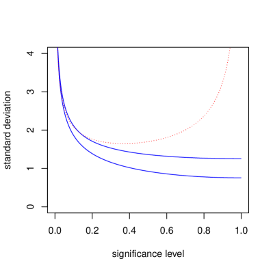
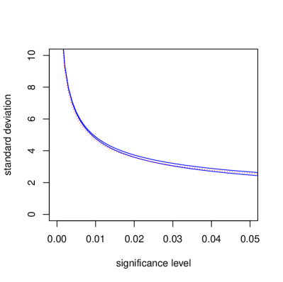
Figure 1: The limits for the standard deviation in Theorem 2 as a function of $\epsilon\in(0,1)$ (left) and $\epsilon\in(0,0.05]$ (right) shown as solid (blue) lines; the asymptotic expression in (10) shown as a dotted (red) line. In all cases $\sigma=1$.

The assumptions (A1)–(A4) do not involve $a$, and Theorem 2 continues to hold if we set $a:=0$; this can be checked by going through the proof of Theorem 2 in Section 6. Theorem 2 can thus also be considered as an efficiency result about conformalizing the standard non-Bayesian least squares procedure; this procedure outputs precisely $(B_{*},B^{*})$ with $a:=0$ as its prediction intervals (see, e.g., [8], p. 131). The least squares procedure has guaranteed coverage probability under weaker assumptions than BRR (not requiring assumptions about $w$); however, its validity is not conditional, similarly to CRR.

5 Further details of CRR

By the definition of the CRR conformity measure, we can rewrite the conformity scores in (6) as

$$\alpha^{y}_{i}:=\left|\left\{j=1,\ldots,n\mid r^{y}_{j}\geq r^{y}_{i}\right\}\right|\wedge\left|\left\{j=1,\ldots,n\mid r^{y}_{j}\leq r^{y}_{i}\right\}\right|,$$ (11)

where the vector of residuals $(r^{y}_{1},\ldots,r^{y}_{n})^{\prime}$ is $(I_{n}-H_{n})Y^{y}$, $I_{n}$ is the unit $n\times n$ matrix, $H_{n}:=X_{n}(X^{\prime}_{n}X_{n}+aI)^{-1}X^{\prime}_{n}$ is the hat matrix, $X_{n}$ is the overall design matrix (the $n\times p$ matrix whose $i$th row is $x^{\prime}_{i}$, $i=1,\ldots,n$), and $Y^{y}$ is the overall vector of labels with the label of the test object set to $y$ (i.e., $Y^{y}$ is the vector in $\mathbb{R}^{n}$ whose $i$th element is $y^{i}$, $i=1,\ldots,n-1$, and whose $n$th element is $y$). If we modify the definition of CRR replacing (11) by $\alpha^{y}_{i}:=-r^{y}_{i}$, we will obtain the definition of upper CRR; and if we replace (11) by $\alpha^{y}_{i}:=r^{y}_{i}$, we will obtain the definition of lower CRR. It is easy to see that the prediction set $\Gamma$ output by CRR at significance level $\epsilon$ is the intersection of the prediction sets output by upper and lower CRR at significance levels $\epsilon/2$. We will concentrate on upper CRR in the rest of this paper: lower CRR is analogous, and CRR is determined by upper and lower CRR.

Let us represent the upper CRR prediction set in a more explicit form (following [12], Section 2.3). We are given the training sequence $(x_{1},y_{1}),\ldots,(x_{n-1},y_{n-1})$ and a test object $x_{n}$; let $y$ be a postulated label for $x_{n}$ and

$$Y^{y}:=(y_{1},\ldots,y_{n-1},y)^{\prime}=(y_{1},\ldots,y_{n-1},0)^{\prime}+y(0,\ldots,0,1)^{\prime}$$

be the vector of labels. The vector of conformity scores is $-(I_{n}-H_{n})Y^{y}=-A-yB$, where

$$A :=(I_{n}-H_{n})(y_{1},\ldots,y_{n-1},0)^{\prime},$$

$$B :=(I_{n}-H_{n})(0,\ldots,0,1)^{\prime}.$$

The components of $A$ and $B$, respectively, will be denoted by $a_{1},\ldots,a_{n}$ and $b_{1},\ldots,b_{n}$.

If we define

$$S_{i}:=\left\{y\mid-a_{i}-b_{i}y\leq-a_{n}-b_{n}y\right\},$$ (12)

the definition of the p-values can be rewritten as

$$p^{y}:=\frac{\left|\left\{i=1,\ldots,n\mid y\in S_{i}\right\}\right|}{n};$$

remember that the prediction set is defined by (5). As shown (under a slightly different definition of $S_{i}$) in [12], pp. 30–34, the prediction set can be computed efficiently, in time $O(n\ln n)$ in the on-line mode.

6 Proof of Theorem 2

For concreteness, we concentrate on the convergence (7) for the upper ends of the conformal and Bayesian prediction intervals. We split the proof into a series of steps.

Regularizing the rays in upper CRR

The upper CRR looks difficult to analyze in general, since the sets (12) may be rays pointing in the opposite directions. Fortunately, the awkward case $b_{n}\leq b_{i}$ ($i<n$) will be excluded for large $n$ under our assumptions (see Lemma 4 below). The following lemma gives a simple sufficient condition for its absence.

Lemma 3.

Suppose that, for each $c\in\mathbb{R}^{p}\setminus\{0\}$,

$$(c\cdot x_{n})^{2}<\sum_{i=1}^{n-1}(c\cdot x_{i})^{2}+a\left\|c\right\|^{2},$$ (13)

where $\left\|\cdot\right\|$ stands for the Euclidean norm. Then $b_{n}>b_{i}$ for all $i=1,\ldots,n-1$.

Intuitively, in the case of a small $a$, (13) being violated for some $c\neq 0$ means that all $x_{1},\ldots,x_{n-1}$ lie approximately in the same hyperplane, and $x_{n}$ is well outside it. The condition (13) can be expressed by saying that the matrix $\sum_{i=1}^{n-1}x_{i}x^{\prime}_{i}-x_{n}x^{\prime}_{n}+aI$ is positive definite.

Proof.

First we assume $a=0$ (so that ridge regression becomes least squares); an extension to $a\geq 0$ will be easy. In this case $H_{n}$ is the projection matrix onto the column space $\mathcal{C}\subseteq\mathbb{R}^{n}$ of the overall design matrix $X_{n}$ and $I_{n}-H_{n}$ is the projection matrix onto the orthogonal complement $\mathcal{C}^{\perp}$ of $\mathcal{C}$. We can have $b_{n}\leq b_{i}$ for $i<n$ (or even $b_{n}^{2}\leq b_{1}^{2}+\cdots+b_{n-1}^{2}$) only if the angle between $\mathcal{C}^{\perp}$ and the hyperplane $\mathbb{R}^{n-1}\times\{0\}$ is $45^{\circ}$ or less; in other words, if the angle between $\mathcal{C}$ and that hyperplane is $45^{\circ}$ or more; in other words, if there is an element $(c\cdot x_{1},\ldots,c\cdot x_{n})^{\prime}$ of $\mathcal{C}$ such that its last coordinate is $c\cdot x_{n}=1$ and its projection $(c\cdot x_{1},\ldots,c\cdot x_{n-1})^{\prime}$ onto the other coordinates has length at most 1.

To reduce the case $a>0$ to $a=0$ add the $p$ dummy objects $\sqrt{a}e_{i}\in\mathbb{R}^{p}$, $i=1,\ldots,p$, labelled by 0 at the beginning of the training sequence; here $e_{1},\ldots,e_{p}$ is the standard basis of $\mathbb{R}^{p}$. ∎

Lemma 4.

The case $b_{n}\leq b_{i}$ for $i<n$ is excluded from some $n$ on almost surely under (A1)–(A4).

Proof.

We will check that (13) holds from some $n$ on. Let us set, without loss of generality, $a:=0$. Let $\Sigma_{l}:=\frac{1}{l}\sum_{i=1}^{l}x_{i}x^{\prime}_{i}$. Since $\lim_{l\to\infty}\Sigma_{l}=\Sigma$ a.s.,

$$\left|\lambda_{\min}(\Sigma_{l})-\lambda_{\min}(\Sigma)\right|\to 0\quad(l\to\infty)\quad\text{a.s.},$$

where $\lambda_{\min}(\cdot)$ is the smallest eigenvalue of the given matrix. Since $\left\|x_{n}\right\|^{2}/n\to 0$ a.s.,

$$\frac{1}{n-1}\sum_{i=1}^{n-1}(c\cdot x_{i})^{2}=c^{\prime}\Sigma_{n-1}c\geq\lambda_{\min}(\Sigma_{n-1})\left\|c\right\|^{2}\\ >\frac{1}{2}\lambda_{\min}(\Sigma)\left\|c\right\|^{2}>\frac{\left\|c\right\|^{2}\left\|x_{n}\right\|^{2}}{n-1}\geq\frac{(c\cdot x_{n})^{2}}{n-1}$$

for all $c\neq 0$ from some $n$ on. ∎

Simplified upper CRR

Let us now find the upper CRR prediction set under the assumption that $b_{n}>b_{i}$ for all $i<n$ (cf. Lemmas 3 and 4 above). In this case each set (12) is

$$S_{i}=(-\infty,t_{i}],\qquad\text{where }t_{i}:=\frac{a_{i}-a_{n}}{b_{n}-b_{i}},$$

except for $S_{n}:=\mathbb{R}$; notice that only $t_{1},\ldots,t_{n-1}$ are defined. The p-value $p^{y}$ for any potential label $y$ of $x_{n}$ is

$$p^{y}=\frac{\left|\{i=1,\ldots,n\mid y\in S_{i}\}\right|}{n}=\frac{\left|\{i=1,\ldots,n-1\mid t_{i}\geq y\}\right|+1}{n}.$$

Therefore, the upper CRR prediction set at significance level $\epsilon/2$ is the ray

$$(-\infty,t_{(k_{n})}],$$

where $k_{n}:=\lceil(1-\epsilon/2)n\rceil$ and $t_{(k)}=t_{k:(n-1)}$ stands, as usual, for the $k$th order statistic of $t_{1},\ldots,t_{n-1}$.

Proof proper

As before, $X$ stands for the design matrix $X_{n-1}$ based on the first $n-1$ observations. A simple but tedious computation (see Appendix A) gives

$$t_{i}=\frac{a_{i}-a_{n}}{b_{n}-b_{i}}=\hat{y}_{n}+(y_{i}-\hat{y}_{i})\frac{1+g_{n}}{1+g_{i}},$$ (14)

where $g_{i}:=x^{\prime}_{i}(X^{\prime}X+aI)^{-1}x_{n}$ (cf. (3)). The first term in (14) is the centre of the Bayesian prediction interval (4); it does not depend on $i$. We can see that

$$B^{*}-C^{*}=(1+g_{n})\left(z_{\epsilon/2}\sigma-V_{(k_{n})}\right),$$ (15)

where $V_{(k_{n})}$ is the $k_{n}$th order statistic in the series

$$V_{i}:=\frac{r_{i}}{1+g_{i}}$$ (16)

of residuals $r_{i}:=y_{i}-\hat{y}_{i}$ adjusted by dividing by $1+g_{i}$. The behaviour of the order statistics of residuals is well studied: see, e.g., the theorem in [2]. The presence of $1+g_{i}$ complicates the situation, and so we first show that $g_{i}$ is small with high probability.

Lemma 5.

Let $\eta_{1},\eta_{2},\ldots$ be a sequence of IID random variables with a finite second moment. Then $\max_{i=1,\ldots,n}\left|\eta_{i}\right|=o(n^{1/2})$ in probability (and even almost surely) as $n\to\infty$.

Proof.

By the strong law of large numbers the sequence $\frac{1}{n}\sum_{i=1}^{n}\eta_{i}^{2}$ converges a.s. as $n\to\infty$, and so $\eta_{n}^{2}/n\to 0$ a.s. This implies that $\max_{i=1,\ldots,n}\left|\eta_{i}\right|=o(n^{1/2})$ a.s. ∎

Corollary 6.

Under the conditions of the theorem, $\max_{i=1,\ldots,n}\left|g_{i}\right|=o(n^{-1/2})$ in probability.

Proof.

Similarly to the proof of Lemma 4, we have, for almost all sequences $x_{1},x_{2},\ldots$,

$$\max_{i=1,\ldots,n}\left|g_{i}\right|\leq\frac{\left\|x_{n}\right\|\max_{i=1,\ldots,n}\left\|x_{i}\right\|}{\lambda_{\min}(X^{\prime}X+aI)}<2\frac{\left\|x_{n}\right\|\max_{i=1,\ldots,n}\left\|x_{i}\right\|}{(n-1)\lambda_{\min}(\Sigma)}$$

from some $n$ on. It remains to combine this with Lemma 5 and the fact that, by Assumption (A1), $\left\|x_{n}\right\|$ is bounded by a constant with high probability. ∎

Corollary 7.

Under the conditions of the theorem, $n^{1/2}\left(r_{(k_{n})}-V_{(k_{n})}\right)\to 0$ in probability.

Proof.

Suppose that, on the contrary, there are $\epsilon>0$ and $\delta>0$ such that $n^{1/2}\left|r_{(k_{n})}-V_{(k_{n})}\right|>\epsilon$ with probability at least $\delta$ for infinitely many $n$. Fix such $\epsilon$ and $\delta$. Suppose, for concreteness, that, with probability at least $\delta$ for infinitely many $n$, we have $n^{1/2}\left(r_{(k_{n})}-V_{(k_{n})}\right)>\epsilon$, i.e., $V_{(k_{n})}<r_{(k_{n})}-\epsilon n^{-1/2}$. The last inequality implies that $V_{i}<r_{(k_{n})}-\epsilon n^{-1/2}$ for at least $k_{n}$ values of $i$. By the definition (16) of $V_{i}$ this in turn implies that $r_{i}<r_{(k_{n})}-\epsilon n^{-1/2}+g_{i}r_{(k_{n})}$ for at least $k_{n}$ values of $i$. By Corollary 6, however, the last addend is less than $\epsilon n^{-1/2}$ with probability at least $1-\delta$ from some $n$ on (the fact that $r_{(k_{n})}$ is bounded with high probability follows, e.g., from Lemma 8 below). This implies $r_{(k_{n})}<r_{(k_{n})}$ with positive probability from some $n$ on, and this contradiction completes the proof. ∎

The last (and most important) component of the proof is the following version of the theorem in [2], itself a version of the famous Bahadur representation theorem [1].

Lemma 8 ([2], theorem).

Under the conditions of Theorem 2,

$$n^{1/2}\left|\left(r_{(k_{n})}-\zeta_{\alpha}\right)-\frac{\alpha-F_{n}(\zeta_{\alpha})}{f(\zeta_{\alpha})}+\mu^{\prime}(\hat{w}_{n}-w)\right|\to 0\qquad\text{a.s.},$$ (17)

where $F_{n}$ is the empirical distribution function of the noise $\xi_{1},\ldots,\xi_{n-1}$ and $\hat{w}_{n}:=(X^{\prime}X+aI)^{-1}X^{\prime}Y$ is the ridge regression estimate of $w$.

For details of the proof (under our assumptions), see Appendix B.

By (15), Corollary 6, and Slutsky’s lemma (see, e.g., [9], Lemma 2.8), it suffices to prove (7) with the left-hand side replaced by $n^{1/2}(V_{(k_{n})}-z_{\epsilon/2}\sigma)$. Moreover, by Corollary 7 and Slutsky’s lemma, it suffices to prove (7) with the left-hand side replaced by $n^{1/2}(r_{(k_{n})}-z_{\epsilon/2}\sigma)$; this is what we will do.

Lemma 8 holds in the situation where $w$ is a constant vector (the distribution of $w$ is allowed to be degenerate). Let $R$ be a Borel set in $(\mathbb{R}^{p})^{\infty}$ such that (17) holds for all $(x_{1},x_{2},\ldots)\in R$, where the “a.s.” is now interpreted as “for almost all sequences $(\xi_{1},\xi_{2},\ldots)$”. By Lebesgue’s dominated convergence theorem, it suffices to prove (7) with the left-hand side replaced by $n^{1/2}(r_{(k_{n})}-z_{\epsilon/2}\sigma)$ for a fixed $w$ and a fixed sequence $(x_{1},x_{2},\ldots)\in R$. Therefore, we fix $w$ and $(x_{1},x_{2},\ldots)\in R$; the only remaining source of randomness is $(\xi_{1},\xi_{2},\ldots)$. Finally, by the definition of the set $R$, it suffices to prove (7) with the left-hand side replaced by

$$n^{1/2}\frac{\alpha-F_{n}(\zeta_{\alpha})}{f(\zeta_{\alpha})}-n^{1/2}\mu^{\prime}(\hat{w}_{n}-w).$$ (18)

Without loss of generality we will assume that $\frac{1}{n}X^{\prime}_{n}X_{n}\to\Sigma$ as $n\to\infty$ (this extra assumption about $R$ will ensure that Lindeberg’s condition is satisfied below).

Since $\operatorname{\mathbb{E}}(\alpha-F_{n}(\zeta_{\alpha}))=0$ and

$$\operatorname{\textrm{var}}\left(\alpha-F_{n}(\zeta_{\alpha})\right)=\frac{F(\zeta_{\alpha})(1-F(\zeta_{\alpha}))}{n-1}=\frac{\alpha(1-\alpha)}{n-1},$$

where $F$ is the distribution function of $N(0,\sigma^{2})$, we have

$$n^{1/2}\frac{\alpha-F_{n}(\zeta_{\alpha})}{f(\zeta_{\alpha})}\stackrel{{\scriptstyle{\rm law}}}{{\longrightarrow}}N\left(0,\frac{\alpha(1-\alpha)}{f^{2}(\zeta_{\alpha})}\right)\quad(n\to\infty)$$

by the central limit theorem (in its simplest form).

Since $\hat{w}_{n}=(X^{\prime}X+aI)^{-1}X^{\prime}Y$ is the ridge regression estimate,

$$\operatorname{\mathbb{E}}(\hat{w}_{n}-w) =-a(X^{\prime}X+aI)^{-1}w=:\Delta_{n},$$ (19)

$$\operatorname{\textrm{var}}(\hat{w}_{n}) =\sigma^{2}(X^{\prime}X+aI)^{-1}X^{\prime}X(X^{\prime}X+aI)^{-1}=:\Omega_{n}.$$ (20)

Furthermore, for $n\to\infty$

$$n^{1/2}\Delta_{n} =-n^{-1/2}a\left(\frac{X^{\prime}X}{n}+\frac{aI}{n}\right)^{-1}w\sim-n^{-1/2}a\Sigma^{-1}w\to 0,$$

$$n\Omega_{n} =\sigma^{2}\left(\frac{X^{\prime}X}{n}+\frac{aI}{n}\right)^{-1}\frac{X^{\prime}X}{n}\left(\frac{X^{\prime}X}{n}+\frac{aI}{n}\right)^{-1}\to\sigma^{2}\Sigma^{-1}.$$

This gives

$$n^{1/2}\mu^{\prime}(\hat{w}_{n}-w)\stackrel{{\scriptstyle{\rm law}}}{{\longrightarrow}}N\left(0,\sigma^{2}\mu^{\prime}\Sigma^{-1}\mu\right)\quad(n\to\infty)$$

(the asymptotic, and even exact, normality is obvious from the formula for $\hat{w}_{n}$).

Let us now calculate the covariance between the two addends in (18):

$$\operatorname{\textrm{cov}} \left(n^{1/2}\frac{\alpha-F_{n}(\zeta_{\alpha})}{f(\zeta_{\alpha})},-n^{1/2}\mu^{\prime}(\hat{w}_{n}-w)\right)$$

$$=\frac{n}{f(\zeta_{\alpha})}\operatorname{\textrm{cov}}\left(F_{n}(\zeta_{\alpha})-\alpha,\mu^{\prime}(\hat{w}_{n}-w)\right)$$

$$=\frac{n}{(n-1)f(\zeta_{\alpha})}\sum_{i=1}^{n-1}\operatorname{\textrm{cov}}\left(1_{\{\xi_{i}\leq\zeta_{\alpha}\}}-\alpha,\mu^{\prime}(\hat{w}_{n}-w)\right)$$

$$=\frac{n}{(n-1)f(\zeta_{\alpha})}\sum_{i=1}^{n-1}\operatorname{\mathbb{E}}\Bigl{(}\left(1_{\{\xi_{i}\leq\zeta_{\alpha}\}}-\alpha\right)\mu^{\prime}(X^{\prime}X+aI)^{-1}X^{\prime}\xi\Bigr{)},$$

where $\xi=(\xi_{1},\ldots,\xi_{n-1})^{\prime}$ and the last equality uses the decomposition $\hat{w}_{n}-w=\Delta_{n}+(X^{\prime}X+aI)^{-1}X^{\prime}\xi$ with the second addend having zero expected value. Since

$$\operatorname{\mathbb{E}}1_{\{\xi_{i}\leq\zeta_{\alpha}\}}\mu^{\prime}(X^{\prime}X+aI)^{-1}X^{\prime}\xi=\sum_{j=1}^{n-1}\operatorname{\mathbb{E}}1_{\{\xi_{i}\leq\zeta_{\alpha}\}}A_{j}\xi_{j}=\mu_{\alpha}A_{i},$$

where $A_{j}:=\mu^{\prime}(X^{\prime}X+aI)^{-1}x_{j}$, $j=1,\ldots,n-1$, $\mu_{\alpha}:=\operatorname{\mathbb{E}}1_{\{\xi_{i}\leq\zeta_{\alpha}\}}\xi_{i}=\int_{-\infty}^{\zeta_{\alpha}}xf(x)dx$. An easy computation gives $\mu_{\alpha}=-\sigma^{2}f(\zeta_{\alpha})$, and so we have

$$\operatorname{\textrm{cov}}\left(n^{1/2}\frac{\alpha-F_{n}(\zeta_{\alpha})}{f(\zeta_{\alpha})},-n^{1/2}\mu^{\prime}(\hat{w}_{n}-w)\right)=\frac{n}{(n-1)f(\zeta_{\alpha})}\sum_{i=1}^{n-1}\mu_{\alpha}A_{i}\\ =-\sigma^{2}\frac{n}{(n-1)}\sum_{i=1}^{n-1}A_{i}=-\sigma^{2}\mu^{\prime}\left(\frac{1}{n}X^{\prime}X+\frac{a}{n}I\right)^{-1}\bar{x}\to-\sigma^{2}\mu^{\prime}\Sigma^{-1}\mu$$

as $n\to\infty$, where $\bar{x}$ is the arithmetic mean of $x_{1},\ldots,x_{n-1}$. Finally, this implies that (18) converges in law to

$$N\left(0,\frac{\alpha(1-\alpha)}{f^{2}(\zeta_{\alpha})}+\sigma^{2}\mu^{\prime}\Sigma^{-1}\mu-2\sigma^{2}\mu^{\prime}\Sigma^{-1}\mu\right)=N\left(0,\frac{\alpha(1-\alpha)}{f^{2}(\zeta_{\alpha})}-\sigma^{2}\mu^{\prime}\Sigma^{-1}\mu\right);$$

the asymptotic normality of (18) follows from the central limit theorem with Lindeberg’s condition, which holds since (18) is a linear combination of the noise random variables $\xi_{1},\ldots,\xi_{n-1}$ with coefficients whose maximum is $o(1)$ as $n\to\infty$ (this uses the assumption $\frac{1}{n}X^{\prime}_{n}X_{n}\to\Sigma$ made earlier).

A more intuitive (but not necessarily simpler) proof can be obtained by noticing that $\hat{w}_{n}-w$ and the residuals are asymptotically (precisely when $a=0$) independent.

7 Conclusion

The results of this paper are asymptotic; it would be very interesting to obtain their non-asymptotic counterparts. In non-asymptotic settings, however, it is not always true that conformalized ridge regression loses little in efficiency as compared with the Bayesian prediction interval; this is illustrated in [12], Section 8.5, and illustrated and explained in [13]. The main difference is that CRR and Bayesian predictor start producing informative predictions after seeing a different number of observations. CRR, like any other conformal predictor (or any other method whose validity depends only on the IID assumption), starts producing informative predictions only after the number of observations exceeds the inverse significance level $1/\epsilon$. After this theoretical lower bound is exceeded, however, the difference between CRR and Bayesian predictions quickly becomes very small.

Another interesting direction of further research is to extend our results to kernel ridge regression.

Acknowledgements

We are grateful to Albert Shiryaev for inviting us in September 2013 to Kolmogorov’s dacha in Komarovka, where this project was conceived, and to Glenn Shafer for his advice about terminology. This work was supported in part by EPSRC (grant EP/K033344/1).

Appendix A Various computations

For the reader’s convenience, this appendix provides details of various routine calculations.

A singular $C$ in (9)

Apply (9) to $\Sigma_{\epsilon}:=\Sigma+\epsilon I$ and $C_{\epsilon}:=C+\epsilon I$, where $\epsilon>0$, in place of $\Sigma$ and $C$, respectively, and let $\epsilon\to 0$.

Computing $t_{i}$ for simplified upper CRR

In addition to the notation $X$ for the design matrix $X_{n-1}$ based on the first $n-1$ observations, we will use the notation $H$ for the hat matrix $X(X^{\prime}X+aI)^{-1}X^{\prime}$ based on the first $n-1$ observations and $\bar{H}$ for the hat matrix $X_{n}(X^{\prime}_{n}X_{n}+aI)^{-1}X^{\prime}_{n}$ based on the first $n$ observations; the elements of $H$ will be denoted as $h_{i,j}$ and the elements of $\bar{H}$ as $\bar{h}_{i,j}$; as always, $h_{i}$ stands for the diagonal element $h_{i,i}$. To compute $t_{i}$ we will use the formulas (2.18) in [3].

Since $B$ is the last column of $I_{n}-H_{n}$ and

$$\bar{h}_{n,n}=\frac{x^{\prime}_{n}(X^{\prime}X+aI)^{-1}x_{n}}{1+x^{\prime}_{n}(X^{\prime}X+aI)^{-1}x_{n}},$$

we have

$$b_{n} =1-\frac{x^{\prime}_{n}(X^{\prime}X+aI)^{-1}x_{n}}{1+x^{\prime}_{n}(X^{\prime}X+aI)^{-1}x_{n}},$$

$$b_{i} =\frac{-x^{\prime}_{n}(X^{\prime}X+aI)^{-1}x_{i}}{1+x^{\prime}_{n}(X^{\prime}X+aI)^{-1}x_{n}}.$$

Therefore,

$$b_{n}-b_{i}=\frac{1+x^{\prime}_{n}(X^{\prime}X+aI)^{-1}x_{i}}{1+x^{\prime}_{n}(X^{\prime}X+aI)^{-1}x_{n}}.$$

Next, letting $\hat{y}$ stand for the predictions computed from the first $n-1$ observations,

$$a_{i} =\sum_{j=1,\ldots,n-1:j\neq i}(-\bar{h}_{i,j}y_{j})+(1-\bar{h}_{i,i})y_{i}$$

$$=y_{i}-\sum_{j=1}^{n-1}\bar{h}_{i,j}y_{j}$$

$$=y_{i}-\sum_{j=1}^{n-1}h_{i,j}y_{j}+\sum_{j=1}^{n-1}\frac{x^{\prime}_{i}(X^{\prime}X+aI)^{-1}x_{n}x^{\prime}_{n}(X^{\prime}X+aI)^{-1}x_{j}}{1+x^{\prime}_{n}(X^{\prime}X+aI)^{-1}x_{n}}y_{j}$$

$$=y_{i}-\hat{y}_{i}+\frac{x^{\prime}_{i}(X^{\prime}X+aI)^{-1}x_{n}x^{\prime}_{n}(X^{\prime}X+aI)^{-1}X^{\prime}Y}{1+x^{\prime}_{n}(X^{\prime}X+aI)^{-1}x_{n}}$$

$$=y_{i}-\hat{y}_{i}+\frac{x^{\prime}_{i}(X^{\prime}X+aI)^{-1}x_{n}\hat{y}_{n}}{1+x^{\prime}_{n}(X^{\prime}X+aI)^{-1}x_{n}}$$

for $i<n$, and

$$a_{n} =\sum_{j<n}(-\bar{h}_{n,j}y_{j})=-\sum_{j=1}^{n-1}\frac{x^{\prime}_{j}(X^{\prime}X+aI)^{-1}x_{n}}{1+x^{\prime}_{n}(X^{\prime}X+aI)^{-1}x_{n}}y_{j}$$

$$=-\frac{Y^{\prime}X(X^{\prime}X+aI)^{-1}x_{n}}{1+x^{\prime}_{n}(X^{\prime}X+aI)^{-1}x_{n}}.$$

Therefore,

$$a_{i}-a_{n}=y_{i}-\hat{y}_{i}+\frac{1+x^{\prime}_{i}(X^{\prime}X+aI)^{-1}x_{n}}{1+x^{\prime}_{n}(X^{\prime}X+aI)^{-1}x_{n}}\hat{y}_{n}.$$

This gives

$$t_{i}=(y_{i}-\hat{y}_{i})\frac{1+x^{\prime}_{n}(X^{\prime}X+aI)^{-1}x_{n}}{1+x^{\prime}_{i}(X^{\prime}X+aI)^{-1}x_{n}}+\hat{y}_{n},$$

i.e., (14).

Expressing $\mu_{\alpha}$ via $\zeta_{\alpha}$

First we use the substitution $y:=x^{2}/2\sigma^{2}$ to obtain

$$\frac{1}{\sqrt{2\pi}\sigma}\int_{0}^{\zeta_{\alpha}}e^{-x^{2}/2\sigma^{2}}xdx=\frac{\sigma}{\sqrt{2\pi}}\int_{0}^{\zeta_{\alpha}^{2}/2\sigma^{2}}e^{y}dy=\frac{\sigma}{\sqrt{2\pi}}\left(1-e^{-\zeta_{\alpha}^{2}/2\sigma^{2}}\right).$$ (21)

Replacing $\zeta_{\alpha}$ by $\infty$,

$$\frac{1}{\sqrt{2\pi}\sigma}\int_{0}^{\infty}e^{-x^{2}/2\sigma^{2}}xdx=\frac{\sigma}{\sqrt{2\pi}}.$$ (22)

Finally, subtracting (22) from (21) gives

$$\mu_{\alpha}=\frac{1}{\sqrt{2\pi}\sigma}\int_{-\infty}^{\zeta_{\alpha}}e^{-x^{2}/2\sigma^{2}}xdx=-\frac{\sigma}{\sqrt{2\pi}}e^{-\zeta_{\alpha}^{2}/2\sigma^{2}}=-\sigma^{2}f(\zeta_{\alpha}).$$

Appendix B Proof of Lemma 8

The proof is modelled on the proof of the theorem in Carroll’s technical report [2] and on Section 2 of [1]. We cannot use the result of [2] since our conditions are somewhat different. Following [2], we only consider the case of simple linear regression ($p=1$). We will prove that (17) holds for all $w$, so that $w$ will be a constant vector in $\mathbb{R}^{p}$ throughout the proof.

We start from the speed of convergence in the ridge regression estimate of regression weights. Let $a_{n}:=n^{-1/2}\ln n$.

Lemma 9.

Under our conditions, $\left|\hat{w}_{n}-w\right|=o(a_{n})$ a.s.

Proof.

This follows immediately from (19) and (20). ∎

The proof uses the following random variables:

$$G_{n}(x) :=n^{-1}\sum_{i=1}^{n}\Bigl{(}1_{\{r_{i}\leq x\}}-1_{\{\xi_{i}\leq\zeta_{\alpha}\}}-F\bigl{(}x+x_{i}(\hat{w}_{n}-w)\bigr{)}+F(\zeta_{\alpha})\Bigr{)},$$

$$H_{n} :=n^{1/2}\sup_{x\in J_{n}}\left|G_{n}(x)\right|,$$

where $J_{n}:=[\zeta_{\alpha}-a_{n},\zeta_{\alpha}+a_{n}]$ and

$$W_{n}(s,t)=n^{-1/2}\sum_{i=1}^{n}\Bigl{(}1_{\{\xi_{i}\leq\zeta_{\alpha}+a_{n}s+a_{n}tx_{i}\}}-1_{\{\xi_{i}\leq\zeta_{\alpha}\}}-F(\zeta_{\alpha}+a_{n}s+a_{n}tx_{i})+F(\zeta_{\alpha})\Bigr{)}.$$ (23)

Lemma 10.

Under our conditions,

$$\sup\left\{\left|W_{n}(s,t)\right|\mid s,t\in[0,1]\right\}\to 0\quad\text{a.s.}$$ (24)

and, therefore, $H_{n}\to 0$ a.s.

Proof.

Since $r_{i}=\xi_{i}-x_{i}(\hat{w}_{n}-w)$ and $\hat{w}_{n}-w=o(a_{n})$ a.s., it is indeed true that (24) implies $H_{n}\to 0$ a.s.; therefore, we will only prove (24). Let $b_{n}\sim\ln^{2}n$ be a sequence of positive integers. It suffices to consider only $s$ and $t$ of the form $\eta_{r,n}:=r/b_{n}$ for $r=0,\ldots,b_{n}$. To see this, apply Taylor’s expansion: if $\left|s-\eta_{r,n}\right|\leq b_{n}^{-1}$ and $\left|t-\eta_{p,n}\right|\leq b_{n}^{-1}$, then

$$\left|n^{-1}\sum_{i=1}^{n}\left(F(\zeta_{\alpha}+sa_{n}+ta_{n}x_{i})-F(\zeta_{\alpha}+\eta_{r,n}a_{n}+\eta_{p,n}a_{n}x_{i})\right)\right|\\ \leq n^{-1}\sum_{i=1}^{n}f(\zeta^{*})a_{n}b_{n}^{-1}(1+\left|x_{i}\right|)=O(a_{n}b_{n}^{-1})=o(n^{-1/2})\quad\text{a.s.}$$

for some $\zeta^{*}$ (we have used the integrability of $x_{1}$).

For fixed $s$ and $t$ we can apply Bernstein’s inequality (see, e.g., [4], Lemma A.2). Let us fix a sequence $x_{1},x_{2},\ldots$ such that $\frac{1}{n}\sum_{i=1}^{n}x_{i}\to\mu$ (which happens with probability one under our conditions for some $\mu$, namely for $\mu:=\operatorname{\mathbb{E}}(x_{1})$). The cumulative variance (conditional on $x_{1},x_{2},\ldots$) of the addends in (23) does not exceed

$$\sum_{i=1}^{n}(a_{n}s+a_{n}tx_{i})=O(na_{n})$$

a.s. (this again uses the integrability of $x_{1}$); therefore, for any $\epsilon>0$,

$$\operatorname{\mathbb{P}}\left\{\left|W_{n}(s,t)\right|>\epsilon\right\}\leq c_{0}\exp\left(-c_{1}n^{1/4}\right)$$

from some $n$ on, where $c_{0}$ and $c_{1}$ are constants depending on $\epsilon$. The probability that $\left|W_{n}(s,t)\right|>\epsilon$ for some $n\geq N$ and some $s,t$ of the form $\eta_{r,n}$ does not exceed

$$\sum_{n=N}^{\infty}b_{n}^{2}c_{0}\exp\left(-c_{1}n^{1/4}\right)\to 0\quad(N\to\infty)\quad\text{a.s.}$$

This completes the proof of the lemma. ∎

Remember that $k_{n}=\lceil\alpha n\rceil$.

Lemma 11.

From some $n$ on, $r_{(k_{n})}\in J_{n}$ a.s.

Proof.

We will only show that $r_{(k_{n})}\leq\zeta_{\alpha}+a_{n}$ from some $n$ on a.s. Since

$$\operatorname{\mathbb{P}}\left\{r_{(k_{n})}>\zeta_{\alpha}+a_{n}\right\}\leq\operatorname{\mathbb{P}}\left\{\sum_{i=1}^{n}1_{\{\xi_{i}\leq\zeta_{\alpha}+a_{n}+x_{i}(\hat{w}_{n}-w)\}}\leq k_{n}\right\}.$$

By Lemma 9, it suffices to show the existence of an $\epsilon>0$ for which $Q_{N}(\epsilon)\to 0$ as $N\to\infty$, where

$$Q_{N}(\epsilon):=\operatorname{\mathbb{P}}\left\{\sum_{i=1}^{n}1_{\{\xi_{i}\leq\zeta_{\alpha}+a_{n}+ta_{n}x_{i}\}}\leq k_{n}\text{ for some $t\in[0,\epsilon]$ and $n\geq N$}\right\}\\ =\operatorname{\mathbb{P}}\biggl{\{}F_{n}(\zeta_{\alpha}+a_{n})\leq k_{n}/n+n^{-1}\sum_{i=1}^{n}\Bigl{(}F(\zeta_{\alpha}+a_{n})-F(\zeta_{\alpha}+a_{n}+ta_{n}x_{i})\Bigr{)}\\ -n^{-1/2}\left(W_{n}(1,t)-W_{n}(1,0)\right)\text{ for some $t\in[0,\epsilon]$ and $n\geq N$}\biggr{\}}.$$

Using Lemma 10 and the fact that

$$n^{-1}\sum_{i=1}^{n} \Bigl{(}F(\zeta_{\alpha}+a_{n})-F(\zeta_{\alpha}+a_{n}+ta_{n}x_{i})\Bigr{)}$$

$$=-n^{-1}\sum_{i=1}^{n}f(\zeta_{\alpha}+a_{n})ta_{n}x_{i}+O\left(n^{-1}\sum_{i=1}^{n}t^{2}a_{n}^{2}x_{i}^{2}\right)$$

$$=-n^{-1}\sum_{i=1}^{n}f(\zeta_{\alpha})ta_{n}x_{i}+O\left(n^{-1}\sum_{i=1}^{n}ta_{n}^{2}x_{i}\right)+O(a_{n}^{2})$$

$$=-f(\zeta_{\alpha})ta_{n}\mu+O\left((\ln\ln n)^{1/2}n^{-1/2}a_{n}\right)+O(a_{n}^{2})$$

$$=-f(\zeta_{\alpha})ta_{n}\mu+o(n^{-1/2})\quad\text{a.s.}$$

(where $\mu:=\operatorname{\mathbb{E}}(x_{1})$), we obtain

$$Q_{N}(\epsilon)=\operatorname{\mathbb{P}}\Bigl{\{}F_{n}(\zeta_{\alpha}+a_{n})\leq\alpha-ta_{n}\mu f(\zeta_{\alpha})+o(n^{-1/2})\\ \text{ for some $t\in[0,\epsilon]$ and $n\geq N$}\Bigr{\}}.$$

By Hoeffding’s inequality (see, e.g., [4], Lemma A.3), when $\delta>0$ is sufficiently small,

$$\operatorname{\mathbb{P}}\left\{F_{n}(\zeta_{\alpha}+a_{n})\leq\alpha+\delta a_{n}\right\}\leq\exp\left(-cna_{n}^{2}\right)=n^{-c\ln n}$$

for some constant $c>0$. This implies that indeed $Q_{N}(\epsilon)\to 0$ as $N\to\infty$. ∎

Now we can finish the proof of Lemma 8. Let $E_{n}$ be the empirical distribution function of $r_{i}$. Lemma 9 and the second order Taylor expansion imply

$$G_{n}(r_{(k_{n})})=E_{n}(r_{(k_{n})})-F_{n}(\zeta_{\alpha})\\ -n^{-1}\sum_{i=1}^{n}\Bigl{(}F(r_{(k_{n})})+f(r_{(k_{n})})x_{i}(\hat{w}_{n}-w)-F(\zeta_{\alpha})\Bigr{)}+O\left(\frac{1}{n}\sum_{i=1}^{n}x_{i}^{2}\right)o(a_{n}^{2})\\ =E_{n}(r_{(k_{n})})-F_{n}(\zeta_{\alpha})-F(r_{(k_{n})})+F(\zeta_{\alpha})+n^{-1}\sum_{i=1}^{n}f(r_{(k_{n})})x_{i}(\hat{w}_{n}-w)\\ +o(n^{-1/2})\quad\text{a.s.}$$ (25)

Similarly,

$$G_{n}(\zeta_{\alpha})=E_{n}(\zeta_{\alpha})-F_{n}(\zeta_{\alpha})-F(\zeta_{\alpha})+F(\zeta_{\alpha})+n^{-1}\sum_{i=1}^{n}f(\zeta_{\alpha})x_{i}(\hat{w}_{n}-w)\\ +o(n^{-1/2})\quad\text{a.s.}$$ (26)

Subtracting (25) from (26) and using Lemmas 10 and 11 and the fact that $E_{n}(r_{(k_{n})})=k_{n}/n$, we obtain

$$n^{1/2}\left|F(r_{(k_{n})})-F(\zeta_{\alpha})-k_{n}/n+E_{n}(\zeta_{\alpha})\right|\\ \leq n^{1/2}n^{-1}\sum_{i=1}^{n}\left|f(r_{(k_{n})})-f(\zeta_{\alpha})\right|x_{i}(\hat{w}_{n}-w))=o(n^{1/2}a_{n}^{2})\to 0\quad\text{a.s.}$$ (27)

The statement of Lemma 8 can now be obtained by plugging

$$F(r_{(k_{n})})-F(\zeta_{\alpha})=(r_{(k_{n})}-\zeta_{\alpha})f(\zeta_{\alpha})+o(n^{-1/2})\quad\text{a.s.}$$

(which follows from the second order Taylor expansion and Lemma 11) and

$$E_{n}(\zeta_{\alpha})=F_{n}(\zeta_{\alpha})+n^{-1/2}W_{n}(0,a_{n}^{-1}(\hat{w}_{n}-w))\\ +n^{-1}\sum_{i=1}^{n}\Bigl{(}F(\zeta_{\alpha}+x_{i}(\hat{w}_{n}-w))-F(\zeta_{\alpha})\Bigr{)}$$

(which follows from the definition of $W$) into (27). Indeed, the addend involving $W_{n}$ is $o(n^{-1/2})$ a.s. by Lemma 10 and, as we will see momentarily,

$$n^{-1}\sum_{i=1}^{n}\bigl{(}F(\zeta_{\alpha}+x_{i}(\hat{w}_{n}-w))-F(\zeta_{\alpha})\bigr{)}-f(\zeta_{\alpha})\mu(\hat{w}_{n}-w)=o(n^{-1/2})\quad\text{a.s.}$$ (28)

Therefore, it remains to prove (28). By the second order Taylor expansion, the minuend on the left-hand side of (28) can be rewritten as

$$n^{-1}\sum_{i=1}^{n}f\bigl{(}\zeta_{\alpha}\bigr{)}x_{i}(\hat{w}_{n}-w))+O\left(n^{-1}\sum_{i=1}^{n}x_{i}^{2}\right)o(a_{n}^{2})\\ =n^{-1}\sum_{i=1}^{n}f(\zeta_{\alpha})x_{i}(\hat{w}_{n}-w))+o(n^{-1/2})\quad\text{a.s.}$$ (29)

where we have used $a_{n}^{-1}(\hat{w}_{n}-w)\to 0$ a.s. (Lemma 9) and $\operatorname{\mathbb{E}}x_{1}^{2}<\infty$. And the difference between the first addend of (29) and the subtrahend on the left-hand side of (28) is $O(n^{-1}a_{n}(n\ln\ln n)^{1/2})=o(n^{-1/2})$.

References

- [1] R. Raj Bahadur. A note on quantiles in large samples. Annals of Mathematical Statistics, 37:577–580, 1966.
-
[2]
Raymond J. Carroll.
On the distribution of quantiles of residuals in a linear model.
Technical Report Mimeo Series No. 1161, Department of Statistics,
University of North Carolina at Chapel Hill, March 1978.
Available
from
http://www.stat.ncsu.edu/information/library/mimeo.php. - [3] Samprit Chatterjee and Ali S. Hadi. Sensitivity Analysis in Linear Regression. Wiley, New York, 1988.
- [4] László Györfi, Michael Kohler, Adam Krzyżak, and Harro Walk. A Distribution-Free Theory of Nonparametric Regression. Springer, New York, 2002.
- [5] Harold V. Henderson and Shayle R. Searle. On deriving the inverse of a sum of matrices. SIAM Review, 23:53–60, 1981.
- [6] Jing Lei and Larry Wasserman. Distribution free prediction bands for nonparametric regression. Journal of the Royal Statistical Society B, 76:71–96, 2014.
- [7] Ronald H. Randles, Thomas P. Hettmansperger, and George Casella. Introduction to the Special Issue: Nonparametric statistics. Statistical Science, 19:561, 2004.
- [8] George A. F. Seber and Alan J. Lee. Linear Regression Analysis. Wiley, Hoboken, NJ, second edition, 2003.
- [9] Aad W. van der Vaart. Asymptotic Statistics. Cambridge University Press, Cambridge, 1998.
- [10] Vladimir Vovk. Conditional validity of inductive conformal predictors. Machine Learning, 92:349–376, 2013.
- [11] Vladimir Vovk. Kernel ridge regression. In Bernhard Schölkopf, Zhiyuan Luo, and Vladimir Vovk, editors, Empirical Inference: Festschrift in Honour of Vladimir N. Vapnik, chapter 11, pages 105–116. Springer, Berlin, 2013.
- [12] Vladimir Vovk, Alex Gammerman, and Glenn Shafer. Algorithmic Learning in a Random World. Springer, New York, 2005.
- [13] Vladimir Vovk, Ilia Nouretdinov, and Alex Gammerman. On-line predictive linear regression. Annals of Statistics, 37:1566–1590, 2009.
- [14] Larry Wasserman. Frasian inference. Statistical Science, 26:322–325, 2011.